Longitudinal high-dimensional principal components analysis with application to diffusion tensor imaging of multiple sclerosis

Abstract

We develop a flexible framework for modeling high-dimensional imaging data observed longitudinally. The approach decomposes the observed variability of repeatedly measured high-dimensional observations into three additive components: a subject-specific imaging random intercept that quantifies the cross-sectional variability, asubject-specific imaging slope that quantifies the dynamic irreversible deformation over multiple realizations, and a subject-visit-specific imaging deviation that quantifies exchangeable effects between visits. The proposed method is very fast, scalable to studies including ultrahigh-dimensional data, and can easily be adapted to and executed on modest computing infrastructures. The method is applied to the longitudinal analysis of diffusion tensor imaging (DTI) data of the corpus callosum of multiple sclerosis (MS) subjects. The study includes $176$ subjects observed at $466$ visits. For each subject and visit the study contains a registered DTI scan of the corpus callosum at roughly 30,000 voxels.

FLA

, , , , and

TT1Supported by Grant R01NS060910 from the National Institute of Neurological Disorders and Stroke and by Award Number EB012547 from the NIH National Institute of Biomedical Imaging and Bioengineering (NIBIB).

TT2Supported by the German Research Foundation through the Emmy Noether Programme, Grant GR 3793/1-1.

TT3Supported by the Intramural Research Program of the National Institute of Neurological Disorders and Stroke.

1 Introduction

An increasing number of longitudinal studies routinely acquire high-dimensional data, such as brain images or gene expression, at multiple visits. This led to increased interest in generalizing standard models designed for longitudinal data analysis to the case when the observed data are massively multivariate. In this paper we propose to generalize the random intercept random slope mixed effects model to the case when instead of a scalar, one measures a high-dimensional object, such as a brain image. The proposed methods can be applied to longitudinal studies that include high-dimensional imaging observations without missing data that can be unfolded into a long vector.

This paper is motivated by a study of multiple sclerosis (MS) patients [Reich et al. (2010)]. Multiple sclerosis is a degenerative disease of the central nervous system. A hallmark of MS is damage to and degeneration of the myelin sheaths that surround and insulate nerve fibers in the brain. Such damage results in sclerotic plaques that distort the flow of electrical impulses along the nerves to different parts of the body [Raine, McFarland and Hohlfeld (2008)]. MS also affects the neurons themselves and is associated with accelerated brain atrophy.

Our data are derived from a natural history study of $176$ MS cases selected from a population with a wide spectrum of disease severity. Subjects were scanned over a 5-year period up to $10$ times per subject, for a total of 466 scans. The scans have been aligned (registered) using a $12$ degrees of freedom transformation which accounts for rotation, translation, scaling, and shearing, but not for nonlinear deformation. In this study we focus on fractional anisotropy (FA), a useful voxel-level summary of diffusion tensor imaging (DTI), a type of structural Magnetic Resonance Imaging (MRI). FA is viewed as a measure of tissue integrity and is thought to be sensitive both to axon fiber density and myelination in white matter. It is measured on a scale between zero (isotropic diffusion characteristic of fluid-filled cavities) and one (anisotropic diffusion, characteristic of highly ordered white matter fiber bundles) [Mori (2007)].

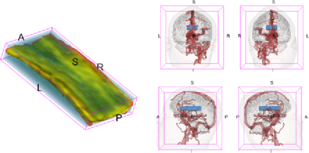
Figure 1: The 3D-rendering of the region of interest (left), a blue block containing corpus callosum, and the template brain (right). Views: R${}={}$Right, L${}={}$Left, S${}={}$Superior, I${}={}$Interior, A${}={}$Anterior, P${}={}$Posterior. For the purposes of orientation, major venous structures are displayed in red in the right half of the template brain. The 3D-renderings are obtained using 3D-Slicer (2011) and 3D reconstructions of the anatomy from Pujol (2010).

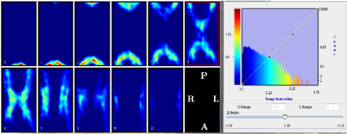
Figure 2: The corpus callosum of a randomly chosen subject. Eleven axial slices are shown on the left. A histogram of the weighted FA values is on the right. Orientation: Interior (slice $0$) to Superior (slice $10$), Posterior (top) to Anterior (bottom), Right to Left. The pictures are obtained using MIPAV (2011).

The goal of the study was to quantify the location and size of longitudinal variability of FA along the corpus callosum. The primary region of interest (ROI) is a central block of the brain containing the corpus callosum, the major bundle of neural fibers connecting the left and right cerebral hemispheres. We weight FA at each voxel in the block with a probability for the voxel to be in the corpus callosum, where the probability is derived from an atlas formed using healthy-volunteer scans, and study longitudinal changes of weighted FAs in the blocks [Reich et al. (2010)]. Figure 1 displays the ROI that contains corpus callosum together with its relative location in a template brain. Each block is of size $38\times 72\times 11$, indicating that there are $38$ sagittal, $72$ coronal, and $11$ axial slices, respectively. Figure 2 displays the $11$ axial (horisontal) slices for one of the subjects from bottom to top. In this paper, we study the FA at every voxel of the blue blocks, which could be unfolded into an approximately $30\mbox{,}000$ dimensional vector that contains the corresponding FA value at each entry. The variability of these images over multiple visits and subjects will be described by the combination of the following: (1) a subject-specific imaging random intercept that quantifies the cross-sectional variability; (2) a subject-specific imaging slope that quantifies the dynamic irreversible deformation over multiple visits; and (3) a subject-visit-specific imaging deviation that quantifies exchangeable or reversible visit-to-visit changes.

High-dimensional data sets have motivated the statistical and imaging communities to develop new methodological approaches to data analysis. Successful modeling approaches involving wavelets and splines and adaptive kernels have been reported in the literature [Bigelow and Dunson (2009), Guo (2002), Hua et al. (2012), Li et al. (2011), Mohamed and Davatzikos (2004), Morris and Carroll (2006), Morris et al. (2011), Reiss and Ogden (2008, 2010), Reiss et al. (2005), Rodríguez, Dunson and Gelfand (2009), Yuan et al. (2014), Zhu, Brown and Morris (2011)]. A different direction of research has focused on principal component decompositions [Di et al. (2009), Crainiceanu, Staicu and Di (2009), Aston, Chiou and Evans (2010), Staicu, Crainiceanu and Carroll (2010), Greven et al. (2010), Di, Crainiceanu and Jank (2010), Zipunnikov et al. (2011a), Crainiceanu et al. (2011)], which led to several applications to imaging data [Shinohara et al. (2011), Goldsmith et al. (2011), Zipunnikov et al. (2011b)]. However, the high dimensionality of new data sets, the inherent complexity of sampling designs and data collection, and the diversity of new technological measurements raise multiple challenges that are currently unaddressed.

Here we address the problem of exploring and analyzing populations of high-dimensional images at multiple visits using high-dimensional longitudinal functional principal components analysis (HD-LFPCA). The method decomposes the longitudinal imaging data into subject-specific, longitudinal subject-specific, and subject-visit-specific components. The dimension reduction for all components is done using principal components of the corresponding covariance operators. Note that we are interested in imaging applications and do not perform smoothing. However, in Section 3.4, we discuss how the proposed approach can be paired with smoothing and applied to high-dimensional functional data. The estimation and inferential methods are fast and can be performed on standard personal computers to analyze hundreds or thousands of high-dimensional images at multiple visits. This was achieved by the following combination of statistical and computational methods: (1) relying only on matrix block calculations and sequential access to memory to avoid loading very large data sets into the computer memory [see Demmel (1997) and Golub and Van Loan (1996) for a comprehensive review of partitioned matrix techniques]; (2) using SVD for matrices that have at least one dimension smaller than $10\mbox{,}000$ [Zipunnikov et al. (2011b)]; (3) obtaining best linear unbiased predictors (BLUPs) of principal scores as a by-product of SVD of the data matrix; and (4) linking the high-dimensional space to a low-dimensional intrinsic space, which allows Karhunen–Loève (KL) decompositions of covariance operators that cannot even be stored in the computer memory. Thus, the proposed methods are computationally linear in the dimension of images.

The rest of the manuscript is organized as follows. Section 2 reviews LFPCA and discusses its limitation in high-dimensional settings. In Section 3 we introduce HD-LFPCA, which provides a new statistical and computational framework for LFPCA. This will circumvent the problems associated with LFPCA in high-dimensional settings. Simulation studies are provided in Section 4. Our methods are applied to the MS data in Section 5. Section 6 concludes the paper with a discussion.

2 Longitudinal FPCA

In this section we review the LFPCA framework introduced by Greven et al. (2010). We develop an estimation procedure based on the original one in Greven et al. (2010), but we heavily modify it to make it practical for applications to imaging high-dimensional data. We also present the major reasons why the original methods cannot be applied to high-dimensional data.

2.1 Model

A brain imaging longitudinal study usually contains a sample of images ${\mathbf{Y}}_{ij}$, where ${\mathbf{Y}}_{ij}$ is a recorded brain image of the $i$th subject, $i=1,\ldots,I$, scanned at times $T_{ij},j=1,\ldots,J_{i}$. The total number of subjects is denoted by $I$. The times $T_{ij}$ are subject specific. Different subjects could have a different number of visits (scans), $J_{i}$. The images are stored in 3-dimensional array structures of dimension $p=p_{1}\times p_{2}\times p_{3}$. For example, in the MS data $p=38\times 72\times 11=30\mbox{,}096$. Note that our approach is not limited to the case when data are in a 3-dimensional array. Instead, it can be applied directly to any data structure where the voxels (or pixels, or locations, etc.) are the same across subjects and visits, and data can be unfolded into a vector. Following Greven et al. (2010), we consider the LFPCA model

$$Y_{ij}(v)=\eta(v)+X_{i,0}(v)+X_{i,1}(v)T_{ij}+W_{ij}(v),$$ (1)

where $v$ denotes a voxel, $\eta(v)$ is a fixed main effect, $X_{i,0}(v)$ is the random imaging intercept for subject $i$, $X_{i,1}(v)$ is the random imaging slope for subject $i$, $T_{ij}$ is the time of visit $j$ for subject $i$, $W_{ij}(v)$ is the random subject/visit-specific imaging deviation. For simplicity, the main effect $\eta(\cdot)$ does not depend on $i$ and $j$. As discussed in Greven et al. (2010), model (1) and the more general model (3.2) in Section 3.2 are similar to functional models with uncorrelated [Guo (2002)] and correlated [Morris and Carroll (2006)] random functional effects. Instead of using smoothing splines and wavelets as in Guo (2002), Morris and Carroll (2006), our approach models the covariance structures using functional principal component analysis; we have found this approach to lead to the major computational advantages, as further discussed in Section 3.

In the remainder of the paper, we unfold the data ${\mathbf{Y}}_{ij}$ and represent it as a $p\times 1$ dimensional vector containing the voxels in a particular order, where the order is preserved across all subjects and visits. We assume that $\eta(v)$ is a fixed surface/image and the latent (unobserved) bivariate process $X_{i}(v)=(X^{\prime}_{i,0}(v),X^{\prime}_{i,1}(v))^{\prime}$ and process $W_{ij}(v)$ are square-integrable stochastic processes. We also assume that $X_{i}(v)$ and $W_{ij}(v)$ are uncorrelated. We denote by ${\mathbf{K}}^{X}(v_{1},v_{2})$ and ${\mathbf{K}}^{W}(v_{1},v_{2})$ their covariance operators, respectively. Assuming that ${\mathbf{K}}^{X}(v_{1},v_{2})$ and ${\mathbf{K}}^{W}(v_{1},v_{2})$ are continuous, we can use the standard Karhunen–Loève expansions of the random processes [Karhunen (1947), Loève (1978)] and represent $X_{i}(v)=\sum_{k=1}^{\infty}\xi_{ik}\phi_{k}^{X}(v)$ with $\phi_{k}^{X}(v)=(\phi_{k}^{X,0}(v),\phi_{k}^{X,1}(v))$ and $W_{ij}(v)=\sum_{l=1}^{\infty}\zeta_{ijl}\phi_{l}^{W}(v)$, where $\phi_{k}^{X}$ and $\phi_{l}^{W}$ are the eigenfunctions of the ${\mathbf{K}}^{X}$ and ${\mathbf{K}}^{W}$ operators, respectively. Note that ${\mathbf{K}}^{X}$ and ${\mathbf{K}}^{W}$ will be estimated by their sample counterparts on finite $2p\times 2p$ and $p\times p$ grids, respectively. Hence, we can always make a working assumption of continuity for ${\mathbf{K}}^{X}$ and ${\mathbf{K}}^{W}$. The LFPCA model becomes the mixed effects model

$$\cases{\displaystyle Y_{ij}(v)=\eta(v)+{\mathbf{Z}}^{\prime}_{ij}\sum_{k=1}^{\infty}\xi_{ik}\phi_{k}^{X}(v)+\sum_{l=1}^{\infty}\zeta_{ijl}\phi_{l}^{W}(v),\vspace*{2pt}\cr(\xi_{ik_{1}},\xi_{ik_{2}})\sim\bigl{(}0,0;\lambda_{k_{1}}^{X},\lambda_{k_{2}}^{X},0\bigr{)};\qquad(\zeta_{ijl_{1}},\zeta_{ijl_{2}})\sim\bigl{(}0,0;\lambda_{l_{1}}^{W},\lambda_{l_{2}}^{W},0\bigr{)},}$$ (2)

where ${\mathbf{Z}}_{ij}=(1,T_{ij})^{\prime}$ and “$\sim(0,0;\lambda_{k_{1}}^{X},\lambda_{k_{2}}^{X},0)$” indicates that a pair of variables is uncorrelated with mean zero and variances $\lambda_{k_{1}}^{X}$ and $\lambda_{k_{2}}^{X}$, respectively. Variances $\lambda^{X}_{k}$’s are nonincreasing, that is, $\lambda^{X}_{k_{1}}\geq\lambda^{X}_{k_{2}}$ if $k_{1}\leq k_{2}$. We do not require normality of the scores in the model. The only assumption is the existence of second order moments of the distribution of scores. In addition, the assumption that $X_{i}(v)$ and $W_{ij}(v)$ are uncorrelated is ensured by the assumption that $\{\xi_{ik}\}_{k=1}^{\infty}$ and $\{\zeta_{ijl}\}_{l=1}^{\infty}$ are uncorrelated. Note that model (2) may be extended to include a more general vector of covariates ${\mathbf{Z}}_{ij}$. We discuss a general functional mixed model in Section 3.2.

In practice, model 2 is projected onto the first $N_{X}$ and $N_{W}$ components of ${\mathbf{K}}^{X}$ and ${\mathbf{K}}^{W}$, respectively. Assuming that $N_{X}$ and $N_{W}$ are known, the model becomes

$$\cases{\displaystyle Y_{ij}(v)=\eta(v)+{\mathbf{Z}}^{\prime}_{ij}\sum_{k=1}^{N_{X}}\xi_{ik}\phi_{k}^{X}(v)+\sum_{l=1}^{N_{W}}\zeta_{ijl}\phi_{l}^{W}(v),\vspace*{2pt}\cr(\xi_{ik_{1}},\xi_{ik_{2}})\sim\bigl{(}0,0;\lambda_{k_{1}}^{X},\lambda_{k_{2}}^{X},0\bigr{)};\qquad(\zeta_{ijl_{1}},\zeta_{ijl_{2}})\sim\bigl{(}0,0;\lambda_{l_{1}}^{W},\lambda_{l_{2}}^{W},0\bigr{)}.}$$ (3)

The choice of the number of principal components $N_{X}$ and $N_{W}$ is discussed in Di et al. (2009), Greven et al. (2010). Typically, $N_{X}$ and $N_{W}$ are small and (3) provides significant dimension reduction of the family of images and their longitudinal dynamics. The main reason why the LFPCA model (3) cannot be fit when data are high dimensional is that the empirical covariance matrices ${\mathbf{K}}^{X}$ and ${\mathbf{K}}^{W}$ cannot be calculated, stored, or diagonalized. Indeed, in our case these operators would be $30\mbox{,}000$ by $30\mbox{,}000$ dimensional, which would have around $1$ billion entries. In other applications these operators would be even bigger.

2.2 Estimation

Our estimation is based on the methods of moments (MoM) for pairwise quadratics $E({\mathbf{Y}}_{ij_{1}}{\mathbf{Y}}_{kj_{2}}^{\prime})$. The computationally intensive part of fitting (3) is estimating the following massively multivariate model:

$${\mathbf{Y}}_{ij} = \eta+\sum_{k=1}^{N_{X}}\xi_{ik}{\bolds\phi}^{X,0}_{k}+T_{ij}\sum_{k=1}^{N_{X}}\xi_{ik}{\bolds\phi}^{X,1}_{k}+\sum_{l=1}^{N_{W}}\zeta_{ijl}{\bolds\phi}^{W}_{l}$$

$$= \eta+\bolds{\Phi}^{X,0}\bolds{\xi}_{i}+T_{ij}\bolds{\Phi}^{X,1}\bolds{\xi}_{i}+\bolds{\Phi}^{W}\bolds{\zeta}_{ij},$$

where $\eta=(\eta(v_{1}),\ldots,\eta(v_{p}))$, ${\mathbf{Y}}_{ij}=\{Y_{ij}(v_{1}),\ldots,Y_{ij}(v_{p})\}$ are $p\times 1$ dimensional vectors, ${\bolds\phi}^{X,0}_{k}$, ${\bolds\phi}^{X,1}_{k}$, and ${\bolds\phi}^{W}_{l}$ are correspondingly vectorized eigenvectors, $\bolds{\Phi}^{X,0}=[{\bolds\phi}^{X,0}_{1},\ldots,{\bolds\phi}^{X,0}_{N_{X}}]$ and $\bolds{\Phi}^{X,1}=[{\bolds\phi}^{X,1}_{1},\ldots,{\bolds\phi}^{X,1}_{N_{X}}]$ are $p\times N_{X}$ dimensional matrices, $\bolds{\Phi}^{W}=[{\bolds\phi}^{W}_{1},\ldots,{\bolds\phi}^{W}_{N_{W}}]$ is a $p\times N_{W}$ dimensional matrix, principal scores $\bolds{\xi}_{i}=(\xi_{i1},\ldots,\xi_{iN_{X}})^{\prime}$ and $\bolds{\zeta}_{ij}=(\zeta_{ij1},\ldots,\zeta_{ijN_{U}})^{\prime}$ are uncorrelated with diagonal covariance matrices $E(\bolds{\xi}_{i}\bolds{\xi}_{i}^{\prime})=\bolds{\Lambda}^{X}={\rm diag}(\lambda^{X}_{1},\ldots,\lambda^{X}_{N_{X}})$ and $E(\bolds{\zeta}_{ij}\bolds{\zeta}_{ij}^{\prime})=\bolds{\Lambda}^{W}={\rm diag}(\lambda^{W}_{1},\ldots,\lambda^{W}_{N_{W}})$, respectively.

To obtain the eigenvectors and eigenvalues in model (2.2), the spectral decompositions of ${\mathbf{K}}^{X}$ and ${\mathbf{K}}^{W}$ need to be constructed. The first $N_{X}$ and $N_{W}$ eigenvectors and eigenvalues are retained after this, that is, ${\mathbf{K}}^{X}\approx\bolds{\Phi}^{X}\bolds{\Lambda}^{X}\bolds{\Phi}^{X^{\prime}}$ and ${\mathbf{K}}^{W}\approx\bolds{\Phi}^{W}\bolds{\Lambda}^{W}\bolds{\Phi}^{W^{\prime}}$, where $\bolds{\Phi}^{X}=[\bolds{\Phi}^{X,0^{\prime}},\bolds{\Phi}^{X,1^{\prime}}]^{\prime}$ denotes a $2p\times N_{X}$ matrix with orthonormal columns and $\bolds{\Phi}^{W}$ is a $p\times N_{W}$ matrix with orthonormal columns.

Lemma 1

The MoM estimators of the covariance operators and the mean in (2.2) are unbiased and given by

$$\hat{{\mathbf{K}}}_{X}^{00} = \sum_{i,j_{1},j_{2}}\widetilde{\mathbf{Y}}_{ij_{1}}\widetilde{\mathbf{Y}}_{ij_{2}}^{\prime}h^{1}_{ij_{1}j_{2}},\qquad\hat{{\mathbf{K}}}_{X}^{01}=\sum_{i,j_{1},j_{2}}\widetilde{\mathbf{Y}}_{ij_{1}}\widetilde{\mathbf{Y}}_{ij_{2}}^{\prime}h^{2}_{ij_{1}j_{2}},$$

$$\hat{{\mathbf{K}}}_{X}^{10} = \sum_{i,j_{1},j_{2}}\widetilde{\mathbf{Y}}_{ij_{1}}\widetilde{\mathbf{Y}}_{ij_{2}}^{\prime}h^{3}_{ij_{1}j_{2}},\qquad\hat{{\mathbf{K}}}_{X}^{11}=\sum_{i,j_{1},j_{2}}\widetilde{\mathbf{Y}}_{ij_{1}}\widetilde{\mathbf{Y}}_{ij_{2}}^{\prime}h^{4}_{ij_{1}j_{2}},$$ (5)

$$\hat{{\mathbf{K}}}^{W} = \sum_{i,j_{1},j_{2}}\widetilde{\mathbf{Y}}_{ij_{1}}\widetilde{\mathbf{Y}}_{ij_{2}}^{\prime}h^{5}_{ij_{1}j_{2}},\qquad\hat{\bolds{\eta}}=\frac{1}{n}\sum_{i=1}^{I}\sum_{j=1}^{J_{i}}{\mathbf{Y}}_{ij},$$

where $\widetilde{\mathbf{Y}}_{ij}={\mathbf{Y}}_{ij}-\hat{\bolds{\eta}}$, the $2p\times 2p$ matrix ${\mathbf{K}}^{X}=[{\mathbf{K}}_{X}^{00}\vdots{\mathbf{K}}_{X}^{01};{\mathbf{K}}_{X}^{10}\vdots{\mathbf{K}}_{X}^{11}]$, with ${\mathbf{K}}_{X}^{ks}=E\{\bolds{\Phi}^{X,k}\bolds{\xi}_{i}(\bolds{\Phi}^{X,s}\bolds{\xi}_{i})^{\prime}\}$ for $k,s\in\{0,1\}$, the weights $h^{l}_{ij_{1}j_{2}}$ are elements of the $l$th column of the matrix ${\mathbf{H}}_{m\times 5}={\mathbf{F}}^{\prime}({\mathbf{F}}{\mathbf{F}}^{\prime})^{-1}$, the matrix ${\mathbf{F}}_{5\times m}$ has columns equal to ${\mathbf{f}}_{ij_{1}j_{2}}=(1,T_{ij_{2}},T_{ij_{1}},T_{ij_{1}}T_{ij_{2}},\delta_{j_{1}j_{2}})^{\prime}$, and $m=\sum_{i=1}^{I}J_{i}^{2}$.

The proof of the lemma is given in the Appendix. The MoM estimators (1) define the symmetric matrices $\hat{{\mathbf{K}}}^{X}$ and $\hat{{\mathbf{K}}}^{W}$. Identifiability of model (2.2) requires that some subjects have more than two visits, that is, $J_{i}\geq 3$. Note that if one is only interested in estimating covariances, $\eta$ can be eliminated as a nuisance parameter by using MoMs for quadratics of differences $E({\mathbf{Y}}_{ij_{1}}-{\mathbf{Y}}_{kj_{2}})({\mathbf{Y}}_{ij_{1}}-{\mathbf{Y}}_{kj_{2}})^{\prime}$ as in Shou et al. (2013).

Estimating the covariance matrices is a crucial first step. However, constructing and storing these matrices requires $O(p^{2})$ calculations and $O(p^{2})$ memory units. Even if it were possible to calculate and store these covariances, obtaining the spectral decompositions would be infeasible. Indeed, ${\mathbf{K}}^{X}$ is a $2p\times 2p$ and ${\mathbf{K}}^{W}$ is a $p\times p$ dimensional matrix, which would require $O(p^{3})$ operations, making diagonalization infeasible for $p>10^{4}$. Therefore, LFPCA, which performs well when the functional dimensionality is moderate, fails in very high and ultrahigh-dimensional settings.

In the next section we develop a methodology capable of handling longitudinal models of very high dimensionality. The main reason why these methods work efficiently is because the intrinsic dimensionality of the model is controlled by the sample size of the study, which is much smaller compared to the number of voxels. The core part of the methodology is to carefully exploit this underlying low-dimensional space.

3 HD-LFPCA

In this section we provide our statistical model and inferential methods. The main emphasis is on providing a new methodological approach with the ultimate goal of solving the intractable computational problems discussed in the previous section.

3.1 Eigenanalysis

In Section 2 we established that the main computational bottleneck for standard LFPCA of Greven et al. (2010) is constructing, storing, and decomposing the relevant covariance operators. In this section we propose an algorithm that allows efficient calculation of the eigenvectors and eigenvalues of these covariance operators without either calculating or storing the covariance operators. In addition, we demonstrate how all necessary calculations can be done using sequential access to data. One of the main assumptions of this section is that the sample size, $n=\sum_{j=1}^{I}J_{i}$, is moderate, so calculations of order $O(n^{3})$ are feasible. In Section 6 we discuss ways to extend our approach to situations when this assumption is violated.

Write $\widetilde{\mathbf{Y}}=(\widetilde{\mathbf{Y}}_{1},\ldots,\widetilde{\mathbf{Y}}_{I})$, where $\widetilde{\mathbf{Y}}_{i}=(\widetilde{\mathbf{Y}}_{i1},\ldots,\widetilde{\mathbf{Y}}_{iJ_{i}})$ is a centered $p\times J_{i}$ matrix and the column $j$, $j=1,\ldots,J_{i}$, contains the unfolded image for subject $i$ at visit $j$. Note that the matrix $\widetilde{\mathbf{Y}}_{i}$ contains all the data for subject $i$ with each column corresponding to a particular visit. The matrix $\widetilde{\mathbf{Y}}$ is the $p\times n$ matrix obtained by column-binding the centered subject-specific data matrices $\widetilde{\mathbf{Y}}_{i}$. Thus, if $\widetilde{\mathbf{Y}}_{i}=(\widetilde{\mathbf{Y}}_{i1},\ldots,\widetilde{\mathbf{Y}}_{iJ_{i}})$, then $\widetilde{\mathbf{Y}}=(\widetilde{\mathbf{Y}}_{1},\ldots,\widetilde{\mathbf{Y}}_{I})$. Our approach starts with constructing the SVD of the matrix $\widetilde{\mathbf{Y}}$:

$$\widetilde{\mathbf{Y}}={\mathbf{V}}{\mathbf{S}}^{1/2}{\mathbf{U}}^{\prime}.$$ (6)

Here, the matrix ${\mathbf{V}}$ is $p\times n$ dimensional with $n$ orthonormal columns, ${\mathbf{S}}$ is a diagonal $n\times n$ dimensional matrix, and ${\mathbf{U}}$ is an $n\times n$ dimensional orthogonal matrix. Calculating the SVD of $\widetilde{\mathbf{Y}}$ requires only a number of operations linear in the number of parameters $p$. Indeed, consider the $n\times n$ symmetric matrix $\widetilde{\mathbf{Y}}^{\prime}\widetilde{\mathbf{Y}}$ with its spectral decomposition $\widetilde{\mathbf{Y}}^{\prime}\widetilde{\mathbf{Y}}={\mathbf{U}}{\mathbf{S}}{\mathbf{U}}^{\prime}$. Note that for high-dimensional $p$ the matrix $\widetilde{\mathbf{Y}}$ cannot be loaded into the memory. The solution is to partition it into $L$ slices as $\widetilde{\mathbf{Y}}^{\prime}=[(\widetilde{\mathbf{Y}}^{1})^{\prime}|(\widetilde{\mathbf{Y}}^{2})^{\prime}|\cdots|(\widetilde{\mathbf{Y}}^{L})^{\prime}]$, where the size of the $l$th slice, $\widetilde{\mathbf{Y}}^{l}$, is $(p/L)\times n$ and can be adapted to the available computer memory and optimized to reduce implementation time. The matrix $\widetilde{\mathbf{Y}}^{\prime}\widetilde{\mathbf{Y}}$ is then calculated as $\sum_{l=1}^{L}(\widetilde{\mathbf{Y}}^{l})^{\prime}\widetilde{\mathbf{Y}}^{l}$ by streaming the individual blocks. This step calculates singular value decomposition of the $p\times n$ matrix $\tilde{\mathbf{Y}}$. Note that for any permutation of components $v$, model (3) will be valid and the covariance structure imposed by the model can be recovered by doing the inverse permutation. If smoothing of the covariance matrix is desirable, then this step can be efficiently combined with Fast Covariance Estimation [FACE, Xiao et al. (2013)], a computationally efficient smoother of (low-rank) high-dimensional covariance matrices with $p$ up to 100,000.

From the SVD (6) the $p\times n$ matrix ${\mathbf{V}}$ can be obtained as ${\mathbf{V}}=\widetilde{\mathbf{Y}}{\mathbf{U}}{\mathbf{S}}^{-1/2}$. The actual calculations can be performed on the slices of the partitioned matrix $\widetilde{\mathbf{Y}}$ as ${\mathbf{V}}^{l}=\widetilde{\mathbf{Y}}^{l}{\mathbf{U}}{\mathbf{S}}^{-1/2},l=1,\ldots,L$. The concatenated slices $[({\mathbf{V}}^{1})^{\prime}|\break({\mathbf{V}}^{2})^{\prime}|\cdots|({\mathbf{V}}^{L})^{\prime}]$ form the matrix of the left singular vectors ${\mathbf{V}}^{\prime}$. Therefore, the SVD (6) can be constructed with sequential access to the data $\widetilde{\mathbf{Y}}$ with $p$-linear effort.

After obtaining the SVD of $\widetilde{\mathbf{Y}}$, each image $\widetilde{\mathbf{Y}}_{ij}$ can be represented as $\widetilde{\mathbf{Y}}_{ij}={\mathbf{V}}{\mathbf{S}}^{1/2}{\mathbf{U}}_{ij}$, where ${\mathbf{U}}_{ij}$ is a corresponding column of matrix ${\mathbf{U}}^{\prime}$. Therefore, the vectors $\widetilde{\mathbf{Y}}_{ij}$ differ only through the vector factors ${\mathbf{U}}_{ij}$ of dimension $n\times 1$. Comparing this SVD representation of $\widetilde{\mathbf{Y}}_{ij}$ with the right-hand side of (2.2), it follows that cross-sectional and longitudinal variability controlled by the principal scores $\bolds{\xi}_{i}$, $\bolds{\zeta}_{ij}$, and time variables $T_{ij}$ must be completely determined by the low-dimensional vectors ${\mathbf{U}}_{ij}$. This is the key observation which makes the approach feasible. Below, we provide more intuition behind our approach. The formal argument is presented in Lemma 2.

First, we substitute the left-hand side of (2.2) with its SVD representation of $\widetilde{\mathbf{Y}}_{ij}$ to get ${\mathbf{V}}{\mathbf{S}}^{1/2}{\mathbf{U}}_{ij}=\bolds{\Phi}^{X,0}\bolds{\xi}_{i}+T_{ij}\bolds{\Phi}^{X,1}\bolds{\xi}_{i}+\bolds{\Phi}^{W}\bolds{\zeta}_{ij}$. Now we can multiply by ${\mathbf{V}}^{\prime}$ both sides of the equation to get ${\mathbf{S}}^{1/2}{\mathbf{U}}_{ij}={\mathbf{V}}^{\prime}\bolds{\Phi}^{X,0}\bolds{\xi}_{i}+T_{ij}{\mathbf{V}}^{\prime}\bolds{\Phi}^{X,1}\bolds{\xi}_{i}+{\mathbf{V}}^{\prime}\bolds{\Phi}^{W}\bolds{\zeta}_{ij}$. If we denote ${\mathbf{A}}^{X,0}={\mathbf{V}}^{\prime}\bolds{\Phi}^{X,0}$ of size $n\times N_{X}$, ${\mathbf{A}}^{X,1}={\mathbf{V}}^{\prime}\bolds{\Phi}^{X,1}$ of size $n\times N_{X}$, and ${\mathbf{A}}^{W}={\mathbf{V}}^{\prime}\bolds{\Phi}^{U}$ of size $n\times N_{W}$, we obtain

$${\mathbf{S}}^{1/2}{\mathbf{U}}_{ij}={\mathbf{A}}^{X,0}\bolds{\xi}_{i}+T_{ij}{\mathbf{A}}^{X,1}\bolds{\xi}_{i}+{\mathbf{A}}^{W}\bolds{\zeta}_{ij}.$$ (7)

Conditionally on the observed data, $\widetilde{\mathbf{Y}}$, models (2.2) and (7) are equivalent. Indeed, model (2.2) is a linear model for the $n$ vectors $\widetilde{\mathbf{Y}}_{ij}$’s. These vectors span an (at most) $n$-dimensional linear subspace. Hence, the columns of the matrix ${\mathbf{V}}$, the right singular vectors of $\widetilde{\mathbf{Y}}$, could be thought of as an orthonormal basis, while ${\mathbf{S}}^{1/2}{\mathbf{U}}_{ij}$ are the coordinates of $\widetilde{\mathbf{Y}}_{ij}$ in this basis. Multiplication by ${\mathbf{V}}^{\prime}$ can be seen as a linear mapping from model (2.2) for the high-dimensional observed data $\widetilde{\mathbf{Y}}_{ij}^{\prime}s$ to model (7) for the low-dimensional data ${\mathbf{S}}^{1/2}{\mathbf{U}}_{ij}$. Additionally, even though ${\mathbf{V}}{\mathbf{V}}^{\prime}\neq{\mathbf{I}}_{p}$, the projection defined by ${\mathbf{V}}$ is lossless in the sense that model (2.2) can be recovered from model (7) using the identity ${\mathbf{V}}{\mathbf{V}}^{\prime}\widetilde{\mathbf{Y}}_{ij}=\widetilde{\mathbf{Y}}_{ij}$. Hence, model (7) has an “intrinsic” dimensionality induced by the study sample size, $n$. We can estimate the low-dimensional model (7) using the LFPCA methods described in Section 2. This step is now feasible, as it requires only $O(n^{3})$ calculations. The formal result presented below shows that fitting model (7) is an essential step for getting the high-dimensional principal components in $p$-linear time.

Lemma 2

The eigenvectors of the estimated covariance operators (1) can be calculated as $\hat{\bolds{\Phi}}^{X,0}={\mathbf{V}}\hat{\mathbf{A}}^{X,0},\hat{\bolds{\Phi}}^{X,1}={\mathbf{V}}\hat{\mathbf{A}}^{X,1},\hat{\bolds{\Phi}}^{W}={\mathbf{V}}\hat{\mathbf{A}}^{W}$, where the matrices $\hat{\mathbf{A}}^{X,0}$, $\hat{\mathbf{A}}^{X,1}$, $\hat{\mathbf{A}}^{W}$ are obtained from fitting model (7). The estimated matrices of eigenvalues $\hat{\bolds{\Lambda}}^{X}$ and $\hat{\bolds{\Lambda}}^{W}$ are the same for both model (2.2) and model (7).

The proof of the lemma is given in the Appendix. This result is a generalization of the HD-MFPCA result in Zipunnikov et al. (2011a), which was obtained in the case when there is no longitudinal component $\bolds{\Phi}^{X,1}$. In the next section we provide more insights into the intrinsic model (7).

3.2 The general functional mixed model

A natural way to generalize model (3) is to consider the following model:

$${\mathbf{Y}}_{ij} = \eta+Z_{ij,0}\sum_{k=1}^{N_{X}}\xi_{ik}{\bolds\phi}^{X,0}_{k}+Z_{ij,1}\sum_{k=1}^{N_{X}}\xi_{ik}{\bolds\phi}^{X,1}_{k}+\cdots$$

$${}+Z_{ij,q}\sum_{k=1}^{N_{X}}\xi_{ik}{\bolds\phi}^{X,q}_{k}+\sum_{l=1}^{N_{W}}\zeta_{ijl}{\bolds\phi}^{W}_{l},$$

where the $(q+1)$-dimensional vector of covariates ${\mathbf{Z}}_{ij}=(Z_{ij,0},Z_{ij,1},\ldots,Z_{ij,q})$ may include, for instance, polynomial terms of $T_{ij}$ and other covariates of interest.

The fitting approach is essentially the same as the one described for the LFPCA model in Section 3.1. As before, the right singular vectors ${\mathbf{U}}_{ij}$ contain the longitudinal information about $\bolds{\xi}_{i}$, $\bolds{\zeta}_{i}$, and covariates ${\mathbf{Z}}_{ij}$. The following two results are direct generalizations of Lemmas 1 and 2.

Lemma 3

The MoM estimators of the covariance operators and the mean in (3.2) are unbiased and given by

$$\hat{{\mathbf{K}}}_{X}^{ks} = \sum_{i,j_{1},j_{2}}\widetilde{\mathbf{Y}}_{ij_{1}}\widetilde{\mathbf{Y}}_{ij_{2}}^{\prime}h^{1+s+k(q+1)}_{ij_{1}j_{2}},\qquad\hat{{\mathbf{K}}}^{W}=\sum_{i,j_{1},j_{2}}\widetilde{\mathbf{Y}}_{ij_{1}}\widetilde{\mathbf{Y}}_{ij_{2}}^{\prime}h^{(q+1)^{2}+1}_{ij_{1}j_{2}},$$

$$\hat{\bolds{\eta}} = \frac{1}{n}\sum_{i=1}^{I}\sum_{j=1}^{J_{i}}{\mathbf{Y}}_{ij},$$

where $\widetilde{\mathbf{Y}}_{ij}={\mathbf{Y}}_{ij}-\hat{\bolds{\eta}}$, the $(q+1)p\times(q+1)p$ block-matrix ${\mathbf{K}}^{X}$ is composed of $p\times p$ matrices ${\mathbf{K}}_{X}^{ks}=E\{\bolds{\Phi}^{X,k}\bolds{\xi}_{i}(\bolds{\Phi}^{X,s}\bolds{\xi}_{i})^{\prime}\}$ for $k,s\in\{0,1,\ldots,q\}$, the weights $h^{l}_{ij_{1}j_{2}}$ are elements of the $l$th column of matrix ${\mathbf{H}}_{m\times((q+1)^{2}+1)}={\mathbf{F}}^{\prime}({\mathbf{F}}{\mathbf{F}}^{\prime})^{-1}$, the matrix ${\mathbf{F}}_{((q+1)^{2}+1)\times m}$ has columns equal to ${\mathbf{f}}_{ij_{1}j_{2}}=(\operatorname{vec}({\mathbf{Z}}_{ij_{1}}\otimes{\mathbf{Z}}_{ij_{2}}),\delta_{j_{1}j_{2}})^{\prime}$, and $m=\sum_{i=1}^{I}J_{i}^{2}$.

Lemma 4

The eigenvectors of the estimated covariance operators for (3.2) can be calculated as $\hat{\bolds{\Phi}}^{X,k}={\mathbf{V}}\hat{\mathbf{A}}^{X,k},k=0,1,\ldots,q,\hat{\bolds{\Phi}}^{W}={\mathbf{V}}\hat{\mathbf{A}}^{W}$, where the matrices $\hat{\mathbf{A}}^{X,k},k=0,1,\ldots,q$, and $\hat{\mathbf{A}}^{W}$ are obtained from fitting the intrinsic model

$${\mathbf{S}}^{1/2}{\mathbf{U}}_{ij} = Z_{ij,0}\sum_{k=1}^{N_{X}}\xi_{ik}{\mathbf{A}}^{X,0}_{k}+Z_{ij,1}\sum_{k=1}^{N_{X}}\xi_{ik}{\mathbf{A}}^{X,1}_{k}+\cdots$$

$${}+Z_{ij,q}\sum_{k=1}^{N_{X}}\xi_{ik}{\mathbf{A}}^{X,q}_{k}+\sum_{l=1}^{N_{W}}\zeta_{ijl}{\mathbf{A}}^{W}_{l}.$$

The estimated matrices of eigenvalues $\hat{\bolds{\Lambda}}^{X}$ and $\hat{\bolds{\Lambda}}^{W}$ are the same for both model (3.2) and model (4).

3.3 Estimation of principal scores

The principal scores are the coordinates of $\widetilde{\mathbf{Y}}_{ij}$ in the basis defined by the LFPCA model (3.2). In this section we propose an approach to calculating BLUP of the scores that is computationally feasible for samples of high-resolution images.

First, we introduce some notation. In Section 3.1 we showed that the SVD of the matrix $\widetilde{\mathbf{Y}}$ can be written as $\widetilde{\mathbf{Y}}_{i}={\mathbf{V}}{\mathbf{S}}^{1/2}{\mathbf{U}}_{i}^{\prime}$, where the $n\times J_{i}$ matrix ${\mathbf{U}}_{i}^{\prime}$ corresponds to the subject $i$. Model (3.2) can be rewritten as

$$\operatorname{vec}(\widetilde{\mathbf{Y}}_{i})={\mathbf{B}}_{i}\bolds{\omega}_{i},$$ (10)

where ${\mathbf{B}}_{i}=[{\mathbf{B}}_{i}^{X}\vdots{\mathbf{B}}_{i}^{W}]$, ${\mathbf{B}}_{i}^{X}={\mathbf{Z}}_{i,0}\otimes\bolds{\Phi}^{X,0}+{\mathbf{Z}}_{i,1}\otimes\bolds{\Phi}^{X,1}+\cdots+{\mathbf{Z}}_{i,q}\otimes\bolds{\Phi}^{X,q}$, ${\mathbf{B}}_{i}^{W}={\mathbf{I}}_{J_{i}}\otimes\bolds{\Phi}^{W}$, ${\mathbf{Z}}_{i,k}=(Z_{i1,k},\ldots,Z_{iJ_{i},k})^{\prime}$, $\bolds{\omega}_{i}=(\bolds{\xi}_{i}^{\prime},\bolds{\zeta}_{i}^{\prime})^{\prime}$, the subject level principal scores $\bolds{\zeta}_{i}=(\bolds{\zeta}^{\prime}_{i1},\ldots,\bolds{\zeta}_{iJ_{i}}^{\prime})^{\prime}$, $\otimes$ is the Kronecker product of matrices, and operation $\operatorname{vec}(\cdot)$ stacks the columns of a matrix on top of each other. The following lemma contains the main result of this section; it shows how the estimated BLUPs can be calculated for the LFPCA model.

Lemma 5

Under the general LFPCA model (3.2), the estimated best linear unbiased predictor (EBLUP) of $\bolds{\xi}_{i}$ and $\bolds{\zeta}_{i}$ is given by

$$\pmatrix{\hat{\bolds{\xi}}_{i}\vspace*{2pt}\cr\hat{\bolds{\zeta}}_{i}}=\bigl{(}\hat{{\mathbf{B}}}_{i}^{\prime}\hat{{\mathbf{B}}}_{i}\bigr{)}^{-1}\hat{{\mathbf{B}}}_{i}^{\prime}\operatorname{vec}(\widetilde{\mathbf{Y}}_{i}),$$ (11)

where all matrix factors on the right-hand side can be written in terms of the low-dimensional right singular vectors.

The proof of the lemma is given in the Appendix. The EBLUPs calculations are almost instantaneous, as the matrices involved in (11) are low-dimensional and do not depend on the dimension $p$. Section .1 in the Appendix briefly describes how the framework can be adapted to settings with tens or hundreds of thousands images.

3.4 HF-LFPCA model with white noise

The original LFPCA model in Greven et al. (2010) was developed for functional observations and contained an additional white noise term. In this section, we show how the HD-LFPCA framework can be extended to accommodate such a term and how the extended model can be estimated.

We now seek to fit the following model:

$${\mathbf{Y}}_{ij} = \eta+Z_{ij,0}\sum_{k=1}^{N_{X}}\xi_{ik}{\bolds\phi}^{X,0}_{k}+Z_{ij,1}\sum_{k=1}^{N_{X}}\xi_{ik}{\bolds\phi}^{X,1}_{k}+\cdots$$

$${}+Z_{ij,q}\sum_{k=1}^{N_{X}}\xi_{ik}{\bolds\phi}^{X,q}_{k}+\sum_{l=1}^{N_{W}}\zeta_{ijl}{\bolds\phi}^{W}_{l}+\varepsilon_{ij},$$

where $\varepsilon_{ij}$ is a $p$-dimensional white noise variable, that is, $E(\varepsilon_{ij})=0_{p}$ for any $i,j$ and $E(\varepsilon_{i_{1}j_{1}}\varepsilon_{i_{2}j_{2}})=\sigma^{2}\delta_{i_{1}i_{2}}\delta_{j_{1}j_{2}}{\mathbf{I}}_{p}$. The white noise process $\varepsilon_{ij}(v)$ is assumed to be uncorrelated with processes $X_{i}(v)$ and $W_{ij}(v)$.

Lemma 3 applied to (3.4) shows that $\hat{K}^{W}_{\sigma^{2}}=\sum_{i,j_{1},j_{2}}\widetilde{\mathbf{Y}}_{ij_{1}}\widetilde{\mathbf{Y}}_{ij_{2}}^{\prime}h^{(q+1)^{2}+1}_{ij_{1}j_{2}}$ is an unbiased estimator of $K^{W}+\sigma^{2}{\mathbf{I}}_{p}$. To estimate $\sigma^{2}$ in a functional case, we can follow the method in Greven et al. (2010): (i) drop the diagonal elements of $\hat{K}^{W}_{\sigma^{2}}$ and use a bivariate smoother to get $\tilde{K}^{W}_{\sigma^{2}}$, (ii) calculate an estimator $\hat{\sigma}^{2}=\max\{(\operatorname{tr}(\hat{K}^{W}_{\sigma^{2}})-\operatorname{tr}(\tilde{K}^{W}_{\sigma^{2}})/p,0\}$. To make this approach feasible in very high-dimensional settings ($p\sim 100\mbox{,}000$), we can use the fast covariance estimation (FACE) developed in Xiao et al. (2013), a bivariate smoother that scales up linearly with respect to $p$ and preserves the low dimensionality of the estimated covariance operator. Thus, HD-LFPCA remains feasible after smoothing by FACE.

When the observations ${\mathbf{Y}}_{ij}$’s are nonfunctional, the off-diagonal smoothing approach cannot be used. In this case, if one assumes that model (3.4) is low-rank, then $\sigma^{2}$ can be estimated as $(\operatorname{tr}(\hat{K}^{W}_{\sigma^{2}})-\sum_{k=1}^{N_{W}}\hat{\lambda}_{k}^{W})/(p-N_{W})$. Bayesian model selection approaches that estimate both the rank of PCA models and variance $\sigma^{2}$ are discussed in Everson and Roberts (2000) and Minka (2000).

4 Simulations

In this section three simulation studies are used to explore the properties of our proposed methods. In the first study, we replicate several simulation scenarios in Greven et al. (2010) for functional curves, but we focus on using a number of parameters up to two orders of magnitude larger than the ones in the original scenarios. This increase in dimensionality could not be handled by the original LFPCA approach. In the second study, we explore how methods recover $3$D spatial bases when the approach of Greven et al. (2010) cannot be implemented. In the third study, we replicate the unbalanced design in and use time variable $T_{ij}$ from our DTI application and generate data using principal components estimated in Section 5. For each scenario, we simulated $100$ data sets. All three studies were run on a four core i7-2.67 GHz PC with 6 Gb of RAM memory using Matlab 2010a. The software is available upon request.

First scenario (1D, functional curves). We follow Greven et al. (2010) and generate data as follows:

$$\cases{\displaystyle Y_{ij}(v)=\sum_{k=1}^{N_{X}}\xi_{ik}\phi_{k}^{X,0}(v)+T_{ij}\sum_{k=1}^{N_{X}}\xi_{ik}\phi_{k}^{X,1}(v)+\sum_{l=1}^{N_{W}}\zeta_{ijl}\phi_{l}^{W}(v)+\varepsilon_{ij}(v),\vspace*{2pt}\cr\qquad v\in\mathcal{V},\vspace*{2pt}\cr\xi_{ik}\stackrel{{\scriptstyle\mathrm{i.i.d.}}}{{\sim}}0.5N\Bigl{(}-\sqrt{\lambda_{k}^{X}}/2,\lambda_{k}^{X}/2\Bigr{)}+0.5N\Bigl{(}\sqrt{\lambda_{k}^{X}}/2,\lambda_{k}^{X}/2\Bigr{)},\vspace*{2pt}\cr\zeta_{ijl}\stackrel{{\scriptstyle\mathrm{i.i.d.}}}{{\sim}}0.5N\Bigl{(}-\sqrt{\lambda_{l}^{W}}/2,\lambda_{l}^{W}/2\Bigr{)}+0.5N\Bigl{(}\sqrt{\lambda_{l}^{W}}/2,\lambda_{l}^{W}/2\Bigr{)},}$$

where $\xi_{ik}\stackrel{{\scriptstyle\mathrm{i.i.d.}}}{{\sim}}0.5N(-\sqrt{\lambda_{k}^{X}}/2,\lambda_{k}^{X}/2)+0.5N(\sqrt{\lambda_{k}^{X}}/2,\lambda_{k}^{X}/2)$ means that the scores $\xi_{ik}$ are simulated from a mixture of two normals, $N(-\sqrt{\lambda_{k}^{X}}/2,\lambda_{k}^{X}/2)$ and $N(\sqrt{\lambda_{k}^{X}}/2,\lambda_{k}^{X}/2)$ with equal probabilities; a similar notation holds for $\zeta_{ijl}$. The scores $\xi_{ik}$’s and $\zeta_{ijl}$’s are mutually independent. We set $I=100$, $J_{i}=4,i=1,\ldots,I$, and the number of eigenfunctions $N_{X}=N_{W}=4$. The true eigenvalues are the same, $\lambda_{k}^{X}=\lambda_{k}^{W}=0.5^{k-1},k=1,2,3,4$. The orthogonal but not mutually orthogonal bases were

$$\phi^{X,0}_{1}(v) = \sqrt{2/3}\sin(2\pi v),\qquad\phi^{X,1}_{1}(v)=1/2,\qquad\phi^{W}_{1}=\sqrt{4}\phi^{X,1}_{1},$$

$$\phi^{X,0}_{2}(v) = \sqrt{2/3}\cos(2\pi v),\qquad\phi^{X,1}_{2}(v)=\sqrt{3}(2v-1)/2,\qquad\phi^{W}_{2}=\sqrt{4/3}\phi^{X,0}_{1},$$

$$\phi^{X,0}_{3}(v) = \sqrt{2/3}\sin(4\pi v),\qquad\phi^{X,1}_{3}(v)=\sqrt{5}\bigl{(}6v^{2}-6v+1\bigr{)}/2,$$

$$\phi^{W}_{3} = \sqrt{4/3}\phi^{X,0}_{2},$$

$$\phi^{X,0}_{4}(v) = \sqrt{2/3}\cos(4\pi v),\qquad\phi^{X,1}_{4}(v)=\sqrt{7}\bigl{(}20v^{3}-30v^{2}+12v-1\bigr{)}/2,$$

$$\phi^{W}_{4} = \sqrt{4/3}\phi^{X,0}_{3},$$

which are measured on a regular grid of $p$ equidistant points in the interval $[0,1]$. To explore scalability, we consider several grids with an increasing number of sampling points, $p$, equal to $750,3000$, $12\mbox{,}000,24\mbox{,}000,48\mbox{,}000$, and $96\mbox{,}000$. Note that a brute-force extension of the standard LFPCA would be at the edge of feasibility for such a large $p$. For each $i$, the first time $T_{i1}$ is generated from the uniform distribution over interval $(0,1)$ denoted by $U(0,1)$. Then differences $(T_{ij+1}-T_{ij})$ are also generated from $U(0,1)$ for $1\leq j\leq 3$. The times $T_{i1},\ldots,T_{i4}$ are normalized to have sample mean zero and variance one. Although no measurement noise is assumed in model (3), we simulate data that also contains white noise, $\varepsilon_{ij}(v)$. The purpose of this is twofold. First, it is of interest to explore how the presence of white noise affects the performance of methods which do not model it explicitly. Second, the choice of the eigenfunctions in the original simulation scenario of Greven et al. (2010) makes the estimation problem ill-posed if data does not contain white noise. The white noise $\varepsilon_{ij}(v)$ is assumed to be i.i.d. $N(0,\sigma^{2})$ for each $i,j,v$ and independent of all other latent processes. To evaluate different signal-to-noise ratios, we consider values of $\sigma^{2}$ equal to $0.0001,0.0005,0.001,0.005,0.01$. Note that we normalized each of the data generating eigenvectors to have norm one. Thus, the signal-to-noise ratio, $(\sum_{k=1}^{4}\lambda_{k}^{X}+\sum_{k=1}^{4}\lambda_{k}^{W})/(p\sigma^{2})$, ranges from $50$ (for $p=750$ and $\sigma^{2}=0.0001$) to $0.004$ (for $p=96\mbox{,}000$ and $\sigma^{2}=0.01$).

Table 1 and Tables 1 and 2 in the online supplement [Zipunnikov et al. (2014)] report the average $L_{2}$ distances between the estimated and true eigenvectors for $X_{i,0}(v)$, $X_{i,1}(v)$, and $W_{ij}(v)$, respectively. The averages are calculated based on $100$ simulated data sets for each $(p,\sigma^{2})$ combination. Standard deviations are shown in brackets. Three trends are obvious: (i) eigenvectors with larger eigenvalues are estimated with higher accuracy, (ii) larger white noise corresponds to a decreasing accuracy, (iii) for identical levels of white noise, accuracy goes down when the dimension $p$ goes up. Similar trends are observed for average distances between estimated and true eigenvalues reported in Tables 3 and 4. These trends follow from the fact that for any fixed $\sigma^{2}$, the signal-to-noise ratio decreases with increasing $p$ and the performance of the approach quickly deteriorates once the signal-to-noise ratio becomes smaller than one.

Table 1: Based on 100 simulated data sets, average distances between estimated and true eigenvectors of $X_{i,0}(v)$; standard deviations are given in parentheses

$\bolds{(p$,$\sigma^{2})}$	$\bolds{\|\phi^{X,0}_{1}-\hat{\phi}^{X,0}_{1}\|^{2}}$	$\bolds{\|\phi^{X,0}_{2}-\hat{\phi}^{X,0}_{2}\|^{2}}$	$\bolds{\|\phi^{X,0}_{3}-\hat{\phi}^{X,0}_{3}\|^{2}}$	$\bolds{\|\phi^{X,0}_{4}-\hat{\phi}^{X,0}_{4}\|^{2}}$
(750, 1e–04)	$0.034\ (0.048)$	$0.07\ (0.069)$	$0.074\ (0.053)$	$0.081\ (0.07)$
(750, 5e–04)	$0.031\ (0.031)$	$0.055\ (0.051)$	$0.084\ (0.097)$	$0.112\ (0.151)$
(750, 0.001)	$0.035\ (0.039)$	$0.062\ (0.054)$	$0.078\ (0.059)$	$0.139\ (0.206)$
(750, 0.005)	$0.035\ (0.039)$	$0.072\ (0.062)$	$0.096\ (0.063)$	$0.159\ (0.084)$
(750, 0.01)	$0.045\ (0.036)$	$0.079\ (0.054)$	$0.129\ (0.102)$	$0.234\ (0.103)$
(3000, 1e–04)	$0.031\ (0.028)$	$0.064\ (0.118)$	$0.09\ (0.13)$	$0.109\ (0.126)$
(3000, 5e–04)	$0.037\ (0.032)$	$0.065\ (0.048)$	$0.077\ (0.06)$	$0.14\ (0.136)$
(3000, 0.001)	$0.031\ (0.027)$	$0.06\ (0.044)$	$0.087\ (0.062)$	$0.131\ (0.07)$
(3000, 0.005)	$0.058\ (0.035)$	$0.106\ (0.058)$	$0.171\ (0.09)$	$0.324\ (0.096)$
(3000, 0.01)	$0.073\ (0.028)$	$0.142\ (0.048)$	$0.236\ (0.074)$	$0.508\ (0.072)$
(12,000, 1e–04)	$0.031\ (0.028)$	$0.062\ (0.048)$	$0.077\ (0.056)$	$0.134\ (0.165)$
(12,000, 5e–04)	$0.041\ (0.036)$	$0.078\ (0.05)$	$0.121\ (0.069)$	$0.201\ (0.081)$
(12,000, 0.001)	$0.047\ (0.04)$	$0.083\ (0.054)$	$0.164\ (0.114)$	$0.295\ (0.118)$
(12,000, 0.005)	$0.112\ (0.032)$	$0.217\ (0.064)$	$0.44\ (0.216)$	$0.758\ (0.153)$
(12,000, 0.01)	$0.175\ (0.031)$	$0.338\ (0.093)$	$0.554\ (0.132)$	$0.987\ (0.071)$
(24,000, 1e–04)	$0.035\ (0.032)$	$0.066\ (0.049)$	$0.09\ (0.141)$	$0.146\ (0.173)$
(24,000, 5e–04)	$0.055\ (0.045)$	$0.097\ (0.061)$	$0.146\ (0.09)$	$0.266\ (0.098)$
(24,000, 0.001)	$0.07\ (0.038)$	$0.125\ (0.047)$	$0.23\ (0.167)$	$0.43\ (0.15)$
(24,000, 0.005)	$0.183\ (0.049)$	$0.348\ (0.097)$	$0.622\ (0.208)$	$0.998\ (0.11)$
(24,000, 0.01)	$0.295\ (0.043)$	$0.518\ (0.117)$	$0.742\ (0.102)$	$1.184\ (0.07)$
(48,000, 1e–04)	$0.046\ (0.068)$	$0.076\ (0.067)$	$0.103\ (0.059)$	$0.175\ (0.122)$
(48,000, 5e–04)	$0.073\ (0.035)$	$0.13\ (0.056)$	$0.234\ (0.1)$	$0.437\ (0.099)$
(48,000, 0.001)	$0.105\ (0.051)$	$0.183\ (0.065)$	$0.407\ (0.23)$	$0.695\ (0.192)$
(48,000, 0.005)	$0.307\ (0.08)$	$0.532\ (0.151)$	$0.824\ (0.208)$	$1.19\ (0.086)$
(48,000, 0.01)	$0.458\ (0.084)$	$0.712\ (0.1)$	$0.938\ (0.074)$	$1.186\ (0.126)$
(96,000, 1e–04)	$0.045\ (0.033)$	$0.087\ (0.059)$	$0.146\ (0.103)$	$0.246\ (0.107)$
(96,000, 5e–04)	$0.116\ (0.081)$	$0.194\ (0.094)$	$0.431\ (0.268)$	$0.721\ (0.218)$
(96,000, 0.001)	$0.188\ (0.089)$	$0.32\ (0.121)$	$0.787\ (0.339)$	$1.062\ (0.216)$
(96,000, 0.005)	$0.457\ (0.065)$	$0.707\ (0.107)$	$0.954\ (0.125)$	$1.298\ (0.074)$
(96,000, 0.01)	$0.662\ (0.105)$	$0.926\ (0.103)$	$1.116\ (0.075)$	$1.143\ (0.153)$

Figure 1 in the online supplement [Zipunnikov et al. (2014)] displays the true and estimated eigenfunctions for the case when $p=12\mbox{,}000$ and $\sigma^{2}=0.01^{2}$ and shows the complete agreement with Figure 2 in Greven et al. (2010). The boxplots of the estimated eigenvalues are displayed in Figure 3. In Figure 4, panels one and three report the boxplots of and panels two and four display the medians and quantiles of the distribution of the normalized estimated scores, $(\xi_{ik}-\hat{\xi}_{ik})/\sqrt{\lambda^{X}_{k}}$ and $(\zeta_{ijl}-\hat{\zeta}_{ijl})/\sqrt{\lambda^{W}_{l}}$, respectively. This indicates that the estimation procedures provides unbiased estimates.

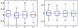
Figure 3: Boxplots of the normalized estimated eigenvalues for process $X_{i}(v)$, $(\hat{\lambda}^{X}_{k}-\lambda^{X}_{k})/\lambda^{X}_{k}$ (left box), and the normalized estimated eigenvalues for process $W_{ij}(v)$, $(\hat{\lambda}^{W}_{l}-\lambda^{W}_{l})/\lambda^{W}_{l}$ (right box), based on scenario $1$ with $100$ replications. The zero is shown by the solid black line.

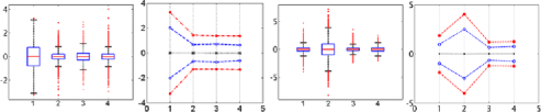
Figure 4: The left two panels show the distribution of the normalized estimated scores of process $X_{i}(v)$, $(\xi_{ik}-\hat{\xi}_{ik})/\sqrt{\lambda^{X}_{k}}$. Boxplots are given in the left column. The right column shows the medians (black marker), $5\%$ and $95\%$ quantiles (blue markers), and $0.5\%$ and $99.5\%$ quantiles (red markers). Similarly, the distribution of the normalized estimated scores of process $W_{ij}(v)$, $(\zeta_{ijl}-\hat{\zeta}_{ijl})/\sqrt{\lambda^{X}_{l}}$ is provided at the right two panels.

Second scenario (3D). Data sets in this study replicate the 3D ROI blocks from the DTI MS data set. We simulated $100$ data sets from the model

$$\cases{\displaystyle Y_{ij}(v)=\sum_{k=1}^{N_{X}}\xi_{ik}\phi_{k}^{X,0}(v)+T_{ij}\sum_{k=1}^{N_{X}}\xi_{ik}\phi_{k}^{X,1}(v)+\sum_{l=1}^{N_{W}}\zeta_{ijl}\phi_{l}^{W}(v),\qquad v\in\mathcal{V},\vspace*{2pt}\cr\xi_{ik}\stackrel{{\scriptstyle\mathrm{i.i.d.}}}{{\sim}}N\bigl{(}0,\lambda_{k}^{X}\bigr{)}\quad\mbox{and}\quad\zeta_{ijl}\stackrel{{\scriptstyle\mathrm{i.i.d.}}}{{\sim}}N\bigl{(}0,\lambda_{l}^{W}\bigr{)},}$$

where $\mathcal{V}=[1,38]\times[1,72]\times[1,11]$. Eigenimages ($\phi^{X,0}_{k}$, $\phi^{X,1}_{k}$) and $\phi^{W}_{l}$ are displayed in Figure 5. The images in this scenario can be thought of as 3D images with voxel intensities on the $[0,1]$ scale. The voxels within each sub-block (eigenimage) are set to $1$ and outside voxels are set to $0$. There are four blue and red sub-blocks corresponding to $\phi^{X,0}_{k}$ and $\phi^{X,1}_{k}$, respectively. The eigenfunctions closest to the anterior side of the brain (labeled A in Figure 1) are $\phi^{X,0}_{1}$ and $\phi^{X,1}_{1}$, which have the strongest signal proportional to the largest eigenvalue (variance), $\lambda^{X}_{1}$. The eigenvectors that are progressively closer to the posterior part of the brain (labeled P) correspond to smaller eigenvalues represented as lighter shades of blue and red, respectively. The sub-blocks closest to the P have the smallest signal, which is proportional to $\lambda^{X}_{4}$. The eigenimages $\phi^{W}_{k}$ shown in green are ordered the same way. Note that $\phi^{X,0}_{k}$ are uncorrelated with $\phi^{W}_{l}$. However, both $\phi^{X,0}_{k}$ and $\phi^{W}_{l}$ are correlated with the $\phi^{X,1}_{k}$’s describing the random slope $X_{i,1}(v)$. We assume that $I=150$, $J_{i}=6,i=1,\ldots,I$, and the true eigenvalues $\lambda_{k}^{X}=0.5^{k-1},k=1,2,3$, and $\lambda_{l}^{W}=0.5^{l-1},l=1,2$. The times $T_{ij}$ were generated as in the first simulation scenario. To apply HD-LFPCA, we unfold each image ${\mathbf{Y}}_{ij}$ and obtain vectors of size $p=38\times 72\times 11=30\mbox{,}096$. The entire simulation study took $20$ minutes or approximately $12$ seconds per data set.

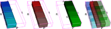
Figure 5: 3D eigenimages of the $2nd$ simulation scenario. From left to right: $\phi^{X,0}_{k}$ are in blue, $\phi^{X,1}_{k}$ are in red, $\phi^{W}_{k}$ are in green, the most right one shows the overlap of all eigenimages. Views: R${}={}$Right, L${}={}$Left, S${}={}$Superior, I${}={}$Interior, A${}={}$Anterior, P${}={}$Posterior. The 3D-renderings are obtained using 3D-Slicer (2011).

Figures 4, 5 and 6 in the online supplement [Zipunnikov et al. (2014)] display the medians of the estimated eigenimages and the voxelwise $5$th and $95$th percentile images, respectively. All axial slices, or $z$ slices in a $x$–$y$–$z$ coordinate system, are the same. Therefore, we display only one $z$-slice, which is representative of the entire 3D image. To obtain a grayscale image with voxel values in the $[0,1]$ interval, each estimated eigenvector, $\hat{{\bolds\phi}}=({\hat{\phi}_{1}},\ldots,{\hat{\phi}_{p}})$, was normalized as $\hat{{\bolds\phi}}\rightarrow(\hat{{\bolds\phi}}-\min_{s}{\hat{\phi}_{s}})/(\max_{s}{\hat{\phi}_{s}}-\min_{s}{\hat{\phi}_{s}})$. Figure 4 in the online supplement [Zipunnikov et al. (2014)] displays the voxelwise medians of the estimator, indicating that the method recovers the spatial configuration of both bases. The $5$-percentile and $95$-percentile images are displayed in Figures 5 and 6 in the online supplement [Zipunnikov et al. (2014)], respectively. Overall, the original pattern is recovered with some small distortions most likely due to the correlation between bases (please note the light gray patches).

The boxplots of the estimated normalized eigenvalues $(\hat{\lambda}^{X}_{k}-\lambda^{X}_{k})/\lambda^{X}_{k}$ and $(\hat{\lambda}^{W}_{l}-\lambda^{W}_{l})/\lambda^{W}_{l}$ are displayed in Figure 2 in the online supplement [Zipunnikov et al. (2014)]. The eigenvalues are estimated consistently. However, in $6$ out of $100$ cases (extreme values shown in red), the estimation procedure did not distinguish well between $\phi^{W}_{3}$ and $\phi^{W}_{4}$. This is probably due the relatively low signal.

The boxplots of the estimated eigenscores are displayed in Figure 3 in the online supplement [Zipunnikov et al. (2014)]. In this scenario, the total number of the estimated scores $\xi_{ik}$ is $15\mbox{,}000$ for each $k$ and there are $90\mbox{,}000$ estimated scores $\zeta_{ijl}$ for each $l$. The distributions of the normalized estimated scores $(\xi_{ik}-\hat{\xi}_{ik})/\sqrt{\lambda^{X}_{k}}$ and $(\zeta_{ijl}-\hat{\zeta}_{ijl})/\sqrt{\lambda^{W}_{l}}$ are displayed in the first and third panels of Figure 3 in the online supplement [Zipunnikov et al. (2014)], respectively. The spread of the distributions increases as the signal-to-noise ratio decreases. The second and fourth panels of Figure 3 in the online supplement [Zipunnikov et al. (2014)] display the medians, $0.5\%$, $5\%$, $95\%$, and $99.5\%$ quantiles of the distribution of the normalized estimated scores.

Third scenario (3D, empirical basis). We generate data using the first ten principal components estimated in Section 5. We replicated the unbalanced design of the MS study and used the same time variable $T_{ij}$’s. The principal scores $\xi_{ik}$ and $\zeta_{ijk}$ were simulated as in Scenario 1 with $\lambda_{k}^{X}=\lambda_{k}^{W}=0.5^{k-1},k=1,\ldots,10$. The white noise variance $\sigma^{2}$ was set to $10^{-4}$. Thus, SNR is equal to 1.32. The results are reported in Table 5 in the online supplement [Zipunnikov et al. (2014)]. The average distances between estimated and true eigenvectors for $X_{i}(v)$ and $W_{ij}(v)$ are calculated based on $100$ simulated data sets. Principal components and principal scores become less accurate as the signal-to-noise gets smaller.

5 Longitudinal analysis of brain fractional anisotropy in MS patients

In this section we apply HD-LFPCA to the DTI images of MS patients. The study population included individuals with no, mild, moderate, and severe disability. Over the follow-up period (as long as 5 years in some cases), there was little change in the median disability level of the cohort. Cohort characteristics are reported in Table 7 in the online supplement [Zipunnikov et al. (2014)]. The scans have been aligned using a $12$ degrees of freedom transformation, meaning that we accounted for rotation, translation, scaling, and shearing, but not for nonlinear deformation. As described in Section 1, the primary region of interest is a central block of the brain of size $38\times 72\times 11$ displayed in Figure 1. We weighted each voxel in the block with a probability for the voxel to be in the corpus callosum and study longitudinal changes of weighted voxels in the blocks [Reich et al. (2010)]. Probabilities less than $0.05$ were set to zero. Below we model longitudinal variability of the weighted FA at every voxel of the blocks. The entire analysis performed in Matlab 2010a took only $3$ seconds on a PC with a quad core i7-2.67 GHz processor and 6 Gb of RAM memory. First, we unfolded each block into a $30\mbox{,}096$ dimensional vector that contained the corresponding weighted FA values. In addition to high dimensionality, another difficulty of analyzing this study was the unbalanced distribution of scans across subjects (see Table 6 in the online supplement [Zipunnikov et al. (2014)]); this is a typical problem in natural history studies. After forming the data matrix ${\mathbf{Y}}$, we estimated the overall mean as $\hat{\eta}=\frac{1}{n}\sum_{i=1}^{I}\sum_{j=1}^{J_{i}}{\mathbf{Y}}_{ij}$ and de-meaned the data. The estimated mean is shown in Figure 7 in the online supplement [Zipunnikov et al. (2014)]. The mean image across subjects and visits indicates a shape characterized by our scientific collaborators as a “standard corpus callosum template.”

Model 1: First, we start by fitting a random intercept and random slope model (1). To enable comparison of the variability explained by processes $X_{i}(v)$ and $W_{ij}(v)$, we followed the normalization procedure in Section 3.4 in Greven et al. (2010): $T_{ij}$’s were normalized to have sample mean zero and sample variance one. The estimated covariance matrices are not necessarily nonnegative definite. Indeed, we have obtained small negative eigenvalues of the covariance operators $\hat{\mathbf{K}}^{X}$ and $\hat{\mathbf{K}}^{W}$. Following Hall, Müller and Yao (2008), all the negative eigenvalues were set to zero. The total variation was decomposed into the “subject-specific” part modeled by process $X_{i}$ and the “exchangeable visit-to-visit” part modeled by the process $W_{ij}$. Most of the total variability, $70.8\%$, is explained by $X_{i}$ (subject-specific variability) with the trace of ${\mathbf{K}}^{X}=122.53$, while $29.2\%$ is explained by $W_{ij}$ (exchangeable visit-to-visit variability) with the trace of ${\mathbf{K}}^{W}=50.47$. Two major contributions of our approach are to separate the processes $X_{i}$ and $W_{ij}$ and quantify their corresponding contributions to the total variability.

Table 2: Model 1 ($T_{ij}$ change): Cumulative variability explained by the first $10$ eigenimages

$\bolds{k}$	$\bolds{\phi_{k}^{X,0}}$	$\bolds{\phi_{k}^{X,1}}$	$\bolds{\phi_{k}^{W}}$	Cumulative
1	$22.13$	0.08	7.12	29.33
2	$10.66$	0.11	3.20	43.29
3	$5.99$	0.13	2.04	51.44
4	$4.84$	0.08	1.44	57.80
5	$2.80$	0.06	0.90	61.56
6	$2.39$	0.07	0.83	64.85
7	$1.94$	0.10	0.63	67.52
8	$1.72$	0.08	0.50	69.82
9	$1.55$	0.05	0.45	71.86
10	$1.20$	0.05	0.39	73.50
	$55.20$	0.80	17.50	73.50

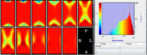
Figure 6: Eleven slices of $\hat{\phi}^{X,0}_{1}$. A histogram of the voxel intensities is on the right. The pictures are obtained using MIPAV (2011).

Figure 7: Eleven slices of $\hat{\phi}^{X,1}_{1}$. A histogram of the voxel intensities is on the right. The pictures are obtained using MIPAV (2011).

Table 2 reports the percentage explained by the first $10$ eigenimages. The first $10$ random intercept eigenimages explain roughly $55\%$ of the total variability, while the effect of the random slope is accounting for only $0.80\%$ of the total variability. The exchangeable variability captured by $W_{ij}(v)$ accounts for $17.5\%$ of the total variation.

The first three estimated random intercept and slope eigenimages are shown in pairs in Figures 6, 7, and in 8, 9, 10, 11 in the online supplement [Zipunnikov et al. (2014)], respectively. Figures 12, 13 and 14 in the online supplement [Zipunnikov et al. (2014)] display the first three eigenimages of the exchangeable measurement error process $W_{ij}(v)$. Each eigenimage is accompanied with the histogram of its voxel values. Recall that the eigenimages were obtained by folding the unit length eigenvectors of $p\approx 3\cdot 10^{4}$ voxels. Therefore, each voxel is represented by a small value. For principal scores, negative and positive voxel values correspond to opposite loadings (directions) of variation. Each histogram has a peak at zero due to the existence of the threshold for the probability maps indicating if a voxel is in the corpus callosum. This peak is a convenient visual divider of the color spectrum into the loading specific colors. Because of the sign invariance of the SVD, the separation between positive and negative loadings is comparable only within the same eigenimage. However, the loadings of the random intercept and slope within an eigenimage of the process $X_{i}(v)$ can be compared as they share the same principal score. This allows us to contrast the time invariant random intercept with the longitudinal random slope and, thus, to localize regions that exhibit the largest longitudinal variability. This could be used to analyze the longitudinal changes of brain imaging in a particular disease or to help generate new scientific hypotheses.

We now interpret the random intercept and slope parts of the eigenimages obtained for the MS data. Figures 6 and 7 show the random intercept and slope parts of the first eigenimage $\phi^{X}_{1}$, respectively. The negatively loaded voxels of the random intercept, $\phi^{X,0}_{1}$, essentially compose the entire corpus callosum. This indicates an overall shift in the mean FA of the corpus callosum. This is expected and is a widely observed empirical feature of principal components. The random slope part, $\phi^{X,1}_{1}$, has both positively and negatively loaded areas in the corpus callosum. The areas colored in blue shades share the sign of the random intercept $\phi^{X,0}_{1}$, whereas the red shades have the opposite sign. The extreme colors of the spectrum of $\phi^{X,1}_{1}$ show a clear separation into negative and positive loadings, especially accentuated in the splenium (posterior) and the genu (anterior) areas of the corpus callosum; please note the upper and lower areas in panels $0$ through $5$ of Figure 7. This implies that a subject with a positive first component score $\xi_{i1}>0$ would tend to have a smaller mean FA over the entire corpus callosum and the FA would tend to decrease with time in the negatively loaded parts of the splenium. The reverse will be true for a subject with a negative score $\xi_{i1}$. The other two eigenimages of $X_{i}(v)$ and eigenimages of $W_{ij}(v)$ are discussed in the online supplement [Zipunnikov et al. (2014)].

Next, we explored whether the deviation process $W_{ij}(v)$ depends on MS severity by analyzing the corresponding eigenscores. To do this, we divided subjects according to their MS type into three subgroups: relapsing-remitting (RR, 102 subjects), secondary progressive (SP, 40 subjects), and primary progressive (PP, 25 subjects). For each of the first ten eigenimages, we formally tested whether there are differences between the distributions of the scores of the three groups using the $t$-test and the Mann–Whitney–Wilcoxon-rank test for equality of means and the Kolmogorov–Smirnov test for equality of distributions. For the first eigenimage, the scores in the SP group have been significantly different from both those in RR and PP groups ($p$-values $<$0.005 for all three tests). For the second eigenimage, scores in the RR group were significantly different from both SP and PP ($p$-values $<$0.01 for all three tests). The two left images of Figure 8 display the group beanplots of the scores for the first eigenimage and the second eigenimage of $W_{ij}(v)$, respectively.

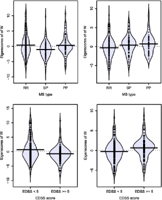
Figure 8: Model 1: Group beanplots according to MS type (top) and according to EDSS score (bottom).

In addition to MS type, the EDSS scores were recorded at each visit. We divided subjects into two groups according to their EDSS score: (i) smaller than 5 and (ii) larger than or equal to 5. As with MS type, we have conducted tests for the equality of distributions of the eigenscores of these two groups for all ten eigenimages. For eigenimages one and two, the distributions of eigenscores have been found to be significantly different ($p$-values $<$0.001 for all three tests). The two right images on Figure 8 display group beanplots of the scores for the first eigenimage and the second eigenimage of $W_{ij}(v)$, respectively.

We have also conducted a standard analysis based on the scalar mean FA over the CC for each subject/visit and fitted a scalar random intercept/random slope model. In this model, the random intercept explains roughly $94\%$ of the total variation of the mean FAs. Figure 15 in the online supplement [Zipunnikov et al. (2014)] displays beanplots of the estimated random intercepts stratified by EDDS score and MS type. For both cases there was a statistically significant difference between the distributions of the random intercepts (EDSS: $p$-values $<0.001$; MS-type, SP vs. RR and PP, $p$-values $<0.002$, for all three tests). Similar tests for the distributions of the random slopes did not identify statistically significant differences between groups. We conclude that this simple model agrees with the full HD-LFPCA mode, though the multivariate model provides a detailed decomposition of the total FA variation together with localization variability in the original 3D-space.

Model 2. Second, we fit model (3.2) using $Z_{ij,1}$ equal to a visit-specific EDSS score. Again, $Z_{ij,1}$’s were normalized to have sample mean 0 and sample variance 1. Table 3 reports percentages explained by the first $10$ eigenimages in model 2. Interestingly, the total variation explained by the random intercept and random slope in both models is approximately the same, with 56.0% in model 1 vs. 54.2% for model 2. However, the random slope in model 2 explains a much higher proportion of the total variation: 13.2% in model 2 using EDSS versus model 1 using time. The second component of the random slope explains almost $8.5\%$ of the total variation. We have also explored whether the scores of $W_{ij}(v)$ depend on MS type and EDSS score using the $t$-test, the Mann–Whitney–Wilcoxon-rank test, and the Kolmogorov–Smirnov test. For the first eigenimage, the SP type was significantly different from the RR ($p$-values $<0.01$ for all three tests), though it was not significantly different from the PP group. For the second eigenimage, the distribution of eigenscores for the SP type was significantly different from that of the scores for the RR ($p$-values $<0.05$ for all three tests), and not significantly different from the distribution of the scores of the PP type. For grouping according to EDSS score, the distributions of the eigenscores of the first two eigenimages have been found to be statistically different ($p$-values $<0.01$ for all three tests). Figure 9 displays beanplots similar to Figure 8 for the distributions of the scores in the groups defined by MS types and EDSS. This indicates that the deviation process $W_{ij}(v)$ in models 1 and 2 carries not only useful but also almost identical remaining information regarding severity of MS.

Table 3: Model 2 ($Z_{ij}$ change): Cumulative variability explained by the first $10$ eigenimages

$\bolds{k}$	$\bolds{\phi_{k}^{X,0}}$	$\bolds{\phi_{k}^{X,1}}$	$\bolds{\phi_{k}^{W}}$	Cumulative
1	$17.79$	0.42	5.59	23.80
2	$0.53$	8.46	1.99	34.78
3	$6.92$	0.39	1.55	43.64
4	$4.68$	0.76	1.05	50.13
5	$3.02$	0.52	0.80	54.46
6	$2.44$	0.29	0.69	57.88
7	$1.63$	0.77	0.54	60.82
8	$1.48$	0.67	0.39	63.36
9	$1.41$	0.51	0.35	65.64
10	$1.19$	0.38	0.33	67.54
	$41.09$	13.17	13.28	67.54

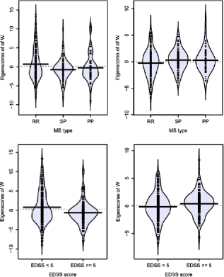
Figure 9: Model 2: Group beanplots according to MS type (top) and according to EDSS score (bottom).

6 Discussion

The methods developed in this paper increase the scope and general applicability of LFPCA to very high-dimensional settings. The base model decomposes the longitudinal data into three main components: a subject-specific random intercept, a subject-specific random slope, and reversible visit-to-visit deviation. We described and addressed computational difficulties that arise with high-dimensional data using a powerful approach referred to as HD-LFPCA. We have developed a procedure designed to identify a low-dimensional space that contains all the information for estimating of the model. This significantly extended the previous related efforts in the clustered functional principal components models, MFPCA [Di et al. (2009)] and HD-MFPCA [Zipunnikov et al. (2011a)].

We applied HD-LFPCA to a novel imaging setting considering DTI and MS in a primary white matter structure. Our investigation characterized longitudinal and cross-sectional variation in the corpus callosum.

There are several outstanding issues for HD-LFPCA that need to be addressed. First, a key assumption of our methods is that they require a moderate sample size that does not exceed ten thousands, or so, images. This limitation can be circumvented by adopting the methods discussed in the Appendix. Second, we have not formally included white noise in our model. Simulation studies in Section 4 demonstrated that a moderate amount of white noise does not have a serious effect on the estimation procedure. However, a more systematic treatment of the related issues is required.

In summary, HD-LFPCA provides a powerful conceptual and practical step toward developing estimation methods for structured ultrahigh-dimensional data.

Appendix

.1 Large sample size

The main assumption which has been made in the paper is that the sample size, $n=\sum_{j=1}^{I}J_{i}$, is sufficiently small to guarantee that calculations of order $O(n^{3})$ are feasible. Below we briefly describe how our framework can be adapted to settings with many more scans—on the order of tens or hundreds of thousands.

LFPCA equation (2.2) models each vector $\widetilde{\mathbf{Y}}_{ij}$ as a linear combination of columns of matrices $\bolds{\Phi}^{X,0}$, $\bolds{\Phi}^{X,1}$, $\bolds{\Phi}^{W}$. Assuming that $2N_{X}+N_{W}<n$, each $\widetilde{\mathbf{Y}}_{ij}$ belongs to an at most $(2N_{X}+N_{W})$-dimensional linear space $\mathfrak{L}(\bolds{\Phi}^{X,0},\bolds{\Phi}^{X,1},\bolds{\Phi}^{W})$ spanned by those columns. Thus, if model (2.2) holds exactly the rank of the matrix, $\widetilde{\mathbf{Y}}$ does not exceed $(2N_{X}+N_{W})$ and at most $2N_{X}+N_{W}$ columns of ${\mathbf{V}}$ correspond to nonzero singular values. This implies that the intrinsic model (7) can be obtained by projecting onto the first $2N_{X}+N_{W}$ columns of ${\mathbf{V}}$ and the sizes of matrices ${\mathbf{A}}^{X,0},{\mathbf{A}}^{X,1},{\mathbf{A}}^{W}$ in (7) will be $(2N_{X}+N_{W})\times N_{X}$, $(2N_{X}+N_{W})\times N_{X}$, and $(2N_{X}+N_{W})\times N_{W}$, respectively. Therefore, the most computationally intensive part would require finding the first $2N_{X}+N_{W}$ left singular vectors of $\widetilde{\mathbf{Y}}$. Of course, in practice, model (2.2) never holds exactly. Hence, the number of columns of matrix ${\mathbf{V}}$ should be chosen to be large enough to either reasonably exceed $(2N_{X}+N_{W})$ or to capture the most variability in data. The latter can be estimated by tracking down the sums of the squares of the corresponding first singular vectors. Thus, this provides a constructive way to handle situations when $n$ is too large to calculate the SVD of $\widetilde{\mathbf{Y}}$.

There are computationally efficient ways to calculate the first $k$ singular vectors of a large matrix. One way is to adapt streaming algorithms [Weng, Zhang and Hwang (2003), Zhao, Yuen and Kwok (2006), Budavari et al. (2009)]. These algorithms usually require only one pass through the data matrix $\widetilde{\mathbf{Y}}$ during which information about the first $k$ singular vectors is accumulated sequentially. Their complexity is of order $O(k^{3}p)$. An alternate approach is to use iterative power methods [see, e.g., Roweis (1997)]. As the dimension of the intrinsic model, $2N_{X}+N_{W}$, is not known in advance, the number of left singular vectors to keep and project onto can be adaptively estimated based on the singular values of the matrix $\widetilde{\mathbf{Y}}$. Further development in this direction is beyond the scope of this paper.

.2 Proofs

Proof of Lemma 1 Using the independence of ${\mathbf{Y}}_{i}$ and ${\mathbf{Y}}_{k}$, the expectation of pairwise quadratics is

$$E\bigl{(}{\mathbf{Y}}_{ij_{1}}{\mathbf{Y}}_{kj_{2}}^{\prime}\bigr{)}$$

(13)

$$\qquad=\cases{{\bolds\eta}{\bolds\eta}^{\prime},\qquad\mbox{if }k\neq i,\vspace*{2pt}\cr{\bolds{\eta}}{\bolds{\eta}}^{\prime}+{\mathbf{K}}_{X}^{00}+T_{ij_{2}}{\mathbf{K}}_{X}^{01}+T_{ij_{1}}{\mathbf{K}}_{X}^{10}+T_{ij_{1}}T_{ij_{2}}{\mathbf{K}}_{X}^{11}+\delta_{j_{1}j_{2}}{\mathbf{K}}^{W},\vspace*{2pt}\cr\hskip 42.0pt\mbox{if }i=k,}$$

where $\delta_{j_{1}j_{2}}$ is $1$ if $j_{1}=j_{2}$ and $0$ otherwise. From the top equality we get the MM estimator of the mean, $\hat{\bolds{\eta}}=n^{-1}\sum_{i,j}{\mathbf{Y}}_{ij}$. The covariances ${\mathbf{K}}^{X}$ and ${\mathbf{K}}^{W}$ can be estimated by de-meaning ${\mathbf{Y}}_{ij}$ as $\widetilde{\mathbf{Y}}_{ij}={\mathbf{Y}}_{ij}-\hat{\bolds{\eta}}$ and regressing $\widetilde{\mathbf{Y}}_{ij_{1}}\widetilde{\mathbf{Y}}_{ij_{2}}^{\prime}$ on $1,T_{ij_{2}},T_{ij_{1}},T_{ij_{1}}T_{ij_{2}}$, and $\delta_{j_{1}j_{2}}$. The bottom equality can be written as $E(\widetilde{\mathbf{Y}}_{ij_{1}j_{2}}^{v})={\mathbf{K}}^{v}{\mathbf{f}}_{ij_{1}j_{2}}$, where $\widetilde{\mathbf{Y}}_{ij_{1}j_{2}}^{v}=\widetilde{\mathbf{Y}}_{ij_{2}}\otimes\widetilde{\mathbf{Y}}_{ij_{1}}$ is a $p^{2}\times 1$ dimensional vector, the parameter of interest is the $p^{2}\times 5$ matrix ${\mathbf{K}}^{v}=[\operatorname{vec}({\mathbf{K}}_{X}^{00}),\operatorname{vec}({\mathbf{K}}_{X}^{01}),\operatorname{vec}({\mathbf{K}}_{X}^{10}),\operatorname{vec}({\mathbf{K}}_{X}^{11})$, $\operatorname{vec}({\mathbf{K}}^{W})]$, and the covariates are entries in the $5\times 1$ vector ${\mathbf{f}}_{ij_{1}j_{2}}=(1,T_{ij_{2}},T_{ij_{1}},T_{ij_{1}}T_{ij_{2}},\delta_{j_{1}j_{2}})^{\prime}$. With this notation $E{\mathbf{Y}}^{v}={\mathbf{K}}^{v}{\mathbf{F}}$, where $\widetilde{\mathbf{Y}}^{v}$ is $p^{2}\times m$ dimensional with $m=\sum_{i=1}^{I}J_{i}^{2}$ and ${\mathbf{F}}$ is a $5\times m$ dimensional matrix with columns equal to ${\mathbf{f}}_{ij_{1}j_{2}},i=1,\ldots,I$ and $j_{1},j_{2}=1,\ldots,J_{i}$. The MM estimator of ${\mathbf{K}}^{v}$ is thus $\hat{\mathbf{K}}^{v}=\widetilde{\mathbf{Y}}^{v}{\mathbf{F}}^{\prime}({\mathbf{F}}{\mathbf{F}}^{\prime})^{-1}$, which provides unbiased estimators of the covariances ${\mathbf{K}}^{X}$ and ${\mathbf{K}}^{W}$. If we denote ${\mathbf{H}}={\mathbf{F}}^{\prime}({\mathbf{F}}{\mathbf{F}}^{\prime})^{-1}$, we get the result of the lemma.

Proof of Lemma 2 Let us denote by $\hat{{\mathbf{K}}}_{{\mathbf{U}}}^{X}$ and $\hat{{\mathbf{K}}}_{{\mathbf{U}}}^{W}$ the matrices defined by equations (1) with ${\mathbf{S}}^{1/2}{\mathbf{U}}_{ij_{1}}{\mathbf{U}}_{ij_{2}}^{\prime}{\mathbf{S}}^{1/2}$ substituted for $\widetilde{\mathbf{Y}}_{ij_{1}}\widetilde{\mathbf{Y}}_{ij_{2}}^{\prime}$. The $2n\times 2n$ dimensional matrix $\hat{{\mathbf{K}}}_{{\mathbf{U}}}^{X}$ and the $n\times n$ dimensional matrix $\hat{{\mathbf{K}}}_{{\mathbf{U}}}^{W}$ are low-dimensional counterparts of $\hat{{\mathbf{K}}}^{X}$ and $\hat{{\mathbf{K}}}^{W}$, respectively. Using the SVD representation $\widetilde{\mathbf{Y}}_{ij}={\mathbf{V}}{\mathbf{S}}^{1/2}{\mathbf{U}}_{ij}$, the estimated high-dimensional covariance matrices can be represented as $\hat{{\mathbf{K}}}^{X}={\mathbf{D}}\hat{{\mathbf{K}}}_{{\mathbf{U}}}^{X}{\mathbf{D}}^{\prime}$ and $\hat{{\mathbf{K}}}^{W}={\mathbf{V}}\hat{{\mathbf{K}}}_{{\mathbf{U}}}^{W}{\mathbf{V}}^{\prime}$, where the matrix ${\mathbf{D}}$ is $2p\times 2n$ dimensional with orthonormal columns defined as

$${\mathbf{D}}=\pmatrix{{\mathbf{V}}&{\mathbf{0}}_{p\times n}\vspace*{2pt}\cr{\mathbf{0}}_{p\times n}&{\mathbf{V}}}.$$ (14)

From the constructive definition of ${\mathbf{H}}$, it follows that the matrices $\hat{{\mathbf{K}}}_{{\mathbf{U}}}^{X}$ and $\hat{{\mathbf{K}}}_{{\mathbf{U}}}^{W}$ are symmetric. Thus, we can construct their spectral decompositions, $\hat{{\mathbf{K}}}_{{\mathbf{U}}}^{X}=\hat{\mathbf{A}}^{X}\hat{\bolds{\Lambda}}^{X}\hat{\mathbf{A}}^{X^{\prime}}$ and $\hat{{\mathbf{K}}}_{{\mathbf{U}}}^{W}=\hat{\mathbf{A}}^{W}\hat{\bolds{\Lambda}}^{W}\hat{\mathbf{A}}^{W^{\prime}}$. Hence, high-dimensional covariance matrices can be represented as $\hat{{\mathbf{K}}}^{X}={\mathbf{D}}\hat{\mathbf{A}}^{X}\hat{\bolds{\Lambda}}^{X}\hat{\mathbf{A}}^{X^{\prime}}{\mathbf{D}}^{\prime}$ and $\hat{{\mathbf{K}}}^{W}={\mathbf{V}}\hat{\mathbf{A}}^{W}\hat{\bolds{\Lambda}}^{W}\hat{\mathbf{A}}^{W^{\prime}}{\mathbf{V}}^{\prime}$, respectively. The result of the lemma now follows from the orthonormality of the columns of matrices ${\mathbf{D}}$ and ${\mathbf{V}}$.

Proof of Lemma 3 With notational changes, the proof is identical to the proof of Lemma 1. Proof of Lemma 4 With notational changes, the proof is identical to the proof of Lemma 2. Proof of Lemma 5 The main idea of the proof is similar to that of Zipunnikov et al. (2011a). We assume that function $\eta(v,T_{ij})=0$. From the model it follows that $\bolds{\omega}_{i}\sim(0,\bolds{\Lambda}_{\bolds{\omega}})$, where $\bolds{\Lambda}_{\bolds{\omega}}$ is a covariance matrix of $\bolds{\omega}_{i}$. When $p\leq N_{X}+J_{i}N_{W}$ the BLUP of $\bolds{\omega}_{i}$ is given by $\hat{\bolds{\omega}}_{i}=\operatorname{Cov}(\bolds{\omega}_{i},\operatorname{vec}(\widetilde{\mathbf{Y}}_{i}))\times\break\operatorname{Var}(\operatorname{vec}(\widetilde{\mathbf{Y}}_{i}))^{-1}\operatorname{vec}(\widetilde{\mathbf{Y}}_{i})=\bolds{\Lambda}_{\bolds{\omega}}{\mathbf{B}}_{i}^{\prime}({\mathbf{B}}_{i}\bolds{\Lambda}_{\bolds{\omega}}{\mathbf{B}}_{i}^{\prime})^{-1}\operatorname{vec}(\widetilde{\mathbf{Y}}_{i})$ [see McCulloch andSearle (2001), Section 9]. The BLUP is essentially a projection and, thus, it does not require any distributional assumptions. It may be defined in terms of a projection matrix. If $\bolds{\xi}_{i}$ and $\bolds{\zeta}_{ij}$ are normal, then the BLUP is the best predictor. When $p>N_{X}+J_{i}N_{W}$ the matrix ${\mathbf{B}}_{i}\bolds{\Lambda}_{\bolds{\omega}}{\mathbf{B}}_{i}^{\prime}$ is not invertible and the generalized inverse of ${\mathbf{B}}_{i}\bolds{\Lambda}_{\bolds{\omega}}{\mathbf{B}}_{i}^{\prime}$ is used [Harville (1976)]. In that case, $\hat{\bolds{\omega}}_{i}=\bolds{\Lambda}_{\bolds{\omega}}{\mathbf{B}}_{i}^{\prime}({\mathbf{B}}_{i}\bolds{\Lambda}_{\bolds{\omega}}{\mathbf{B}}_{i}^{\prime})^{-}\operatorname{vec}(\widetilde{\mathbf{Y}}_{i})=\bolds{\Lambda}_{\bolds{\omega}}^{1/2}(\bolds{\Lambda}_{\bolds{\omega}}^{1/2}{\mathbf{B}}_{i}^{\prime}{\mathbf{B}}_{i}\bolds{\Lambda}_{\bolds{\omega}}^{1/2})^{-1}\bolds{\Lambda}_{\bolds{\omega}}^{1/2}{\mathbf{B}}_{i}^{\prime}\operatorname{vec}(\widetilde{\mathbf{Y}}_{i})=({\mathbf{B}}_{i}^{\prime}{\mathbf{B}}_{i})^{-1}{\mathbf{B}}_{i}^{\prime}\operatorname{vec}(\widetilde{\mathbf{Y}}_{i})$. Note that it coincides with the OLS estimator for $\bolds{\omega}_{i}$ if $\bolds{\omega}_{i}$ were a fixed parameter. Thus, the estimated BLUPs are given by $\hat{\bolds{\omega}}_{i}=(\hat{{\mathbf{B}}}_{i}^{\prime}\hat{{\mathbf{B}}}_{i})^{-1}\hat{{\mathbf{B}}}_{i}^{\prime}\operatorname{vec}(\widetilde{\mathbf{Y}}_{i})$.

References

- 3D-Slicer (2011) {bmisc}[auto:parserefs-M02] \borganization3D-Slicer (\byear2011). \bhowpublishedhttp://www.slicer.org/. \bptokimsref\endbibitem
- Aston, Chiou and Evans (2010) {barticle}[mr] \bauthor\bsnmAston, \bfnmJohn A. D.\binitsJ. A. D., \bauthor\bsnmChiou, \bfnmJeng-Min\binitsJ.-M. and \bauthor\bsnmEvans, \bfnmJonathan P.\binitsJ. P. (\byear2010). \btitleLinguistic pitch analysis using functional principal component mixed effect models. \bjournalJ. R. Stat. Soc. Ser. C. Appl. Stat. \bvolume59 \bpages297–317. \biddoi=10.1111/j.1467-9876.2009.00689.x, issn=0035-9254, mr=2744475 \bptokimsref\endbibitem
- Bigelow and Dunson (2009) {barticle}[mr] \bauthor\bsnmBigelow, \bfnmJamie L.\binitsJ. L. and \bauthor\bsnmDunson, \bfnmDavid B.\binitsD. B. (\byear2009). \btitleBayesian semiparametric joint models for functional predictors. \bjournalJ. Amer. Statist. Assoc. \bvolume104 \bpages26–36. \biddoi=10.1198/jasa.2009.0001, issn=0162-1459, mr=2663031 \bptokimsref\endbibitem
- Budavari et al. (2009) {barticle}[auto:parserefs-M02] \bauthor\bsnmBudavari, \bfnmT.\binitsT., \bauthor\bsnmWild, \bfnmV.\binitsV., \bauthor\bsnmSzalay, \bfnmA. S.\binitsA. S., \bauthor\bsnmDobos, \bfnmL.\binitsL. and \bauthor\bsnmYip, \bfnmC.-W.\binitsC.-W. (\byear2009). \btitleReliable eigenspectra for new generation surveys. \bjournalMonthly Notices of the Royal Astronomical Society \bvolume394 \bpages1496–1502. \bptokimsref\endbibitem
- Crainiceanu, Staicu and Di (2009) {barticle}[mr] \bauthor\bsnmCrainiceanu, \bfnmCiprian M.\binitsC. M., \bauthor\bsnmStaicu, \bfnmAna-Maria\binitsA.-M. and \bauthor\bsnmDi, \bfnmChong-Zhi\binitsC.-Z. (\byear2009). \btitleGeneralized multilevel functional regression. \bjournalJ. Amer. Statist. Assoc. \bvolume104 \bpages1550–1561. \biddoi=10.1198/jasa.2009.tm08564, issn=0162-1459, mr=2750578 \bptokimsref\endbibitem
- Crainiceanu et al. (2011) {barticle}[mr] \bauthor\bsnmCrainiceanu, \bfnmCiprian M.\binitsC. M., \bauthor\bsnmCaffo, \bfnmBrian S.\binitsB. S., \bauthor\bsnmLuo, \bfnmSheng\binitsS., \bauthor\bsnmZipunnikov, \bfnmVadim M.\binitsV. M. and \bauthor\bsnmPunjabi, \bfnmNaresh M.\binitsN. M. (\byear2011). \btitlePopulation value decomposition, a framework for the analysis of image populations. \bjournalJ. Amer. Statist. Assoc. \bvolume106 \bpages775–790. \biddoi=10.1198/jasa.2011.ap10089, issn=0162-1459, mr=2894733 \bptokimsref\endbibitem
- Demmel (1997) {bbook}[mr] \bauthor\bsnmDemmel, \bfnmJames W.\binitsJ. W. (\byear1997). \btitleApplied Numerical Linear Algebra. \bpublisherSIAM, \blocationPhiladelphia, PA. \biddoi=10.1137/1.9781611971446, mr=1463942 \bptokimsref\endbibitem
- Di, Crainiceanu and Jank (2010) {bmisc}[auto:parserefs-M02] \bauthor\bsnmDi, \bfnmC.\binitsC., \bauthor\bsnmCrainiceanu, \bfnmC. M.\binitsC. M. and \bauthor\bsnmJank, \bfnmW. S.\binitsW. S. (\byear2010). \bhowpublishedMultilevel sparse functional principal component analysis. Stat. 3 126–143. \bptokimsref\endbibitem
- Di et al. (2009) {barticle}[mr] \bauthor\bsnmDi, \bfnmChong-Zhi\binitsC.-Z., \bauthor\bsnmCrainiceanu, \bfnmCiprian M.\binitsC. M., \bauthor\bsnmCaffo, \bfnmBrian S.\binitsB. S. and \bauthor\bsnmPunjabi, \bfnmNaresh M.\binitsN. M. (\byear2009). \btitleMultilevel functional principal component analysis. \bjournalAnn. Appl. Stat. \bvolume3 \bpages458–488. \biddoi=10.1214/08-AOAS206, issn=1932-6157, mr=2668715 \bptnotecheck year \bptokimsref\endbibitem
- Everson and Roberts (2000) {barticle}[mr] \bauthor\bsnmEverson, \bfnmRichard\binitsR. and \bauthor\bsnmRoberts, \bfnmStephen\binitsS. (\byear2000). \btitleInferring the eigenvalues of covariance matrices from limited, noisy data. \bjournalIEEE Trans. Signal Process. \bvolume48 \bpages2083–2091. \biddoi=10.1109/78.847792, issn=1053-587X, mr=1824643 \bptokimsref\endbibitem
- Goldsmith et al. (2011) {barticle}[pbm] \bauthor\bsnmGoldsmith, \bfnmJeff\binitsJ., \bauthor\bsnmCrainiceanu, \bfnmCiprian M.\binitsC. M., \bauthor\bsnmCaffo, \bfnmBrian S.\binitsB. S. and \bauthor\bsnmReich, \bfnmDaniel S.\binitsD. S. (\byear2011). \btitlePenalized functional regression analysis of white-matter tract profiles in multiple sclerosis. \bjournalNeuroImage \bvolume57 \bpages431–439. \biddoi=10.1016/j.neuroimage.2011.04.044, issn=1095-9572, mid=NIHMS294019, pii=S1053-8119(11)00443-5, pmcid=3114268, pmid=21554962 \bptokimsref\endbibitem
- Golub and Van Loan (1996) {bbook}[mr] \bauthor\bsnmGolub, \bfnmGene H.\binitsG. H. and \bauthor\bsnmVan Loan, \bfnmCharles F.\binitsC. F. (\byear1996). \btitleMatrix Computations, \bedition3rd ed. \bpublisherJohns Hopkins Univ. Press, \blocationBaltimore, MD. \bidmr=1417720 \bptokimsref\endbibitem
- Greven et al. (2010) {barticle}[mr] \bauthor\bsnmGreven, \bfnmSonja\binitsS., \bauthor\bsnmCrainiceanu, \bfnmCiprian\binitsC., \bauthor\bsnmCaffo, \bfnmBrian\binitsB. and \bauthor\bsnmReich, \bfnmDaniel\binitsD. (\byear2010). \btitleLongitudinal functional principal component analysis. \bjournalElectron. J. Stat. \bvolume4 \bpages1022–1054. \biddoi=10.1214/10-EJS575, issn=1935-7524, mr=2727452 \bptokimsref\endbibitem
- Guo (2002) {barticle}[mr] \bauthor\bsnmGuo, \bfnmWensheng\binitsW. (\byear2002). \btitleFunctional mixed effects models. \bjournalBiometrics \bvolume58 \bpages121–128. \biddoi=10.1111/j.0006-341X.2002.00121.x, issn=0006-341X, mr=1891050 \bptokimsref\endbibitem
- Hall, Müller and Yao (2008) {barticle}[mr] \bauthor\bsnmHall, \bfnmPeter\binitsP., \bauthor\bsnmMüller, \bfnmHans-Georg\binitsH.-G. and \bauthor\bsnmYao, \bfnmFang\binitsF. (\byear2008). \btitleModelling sparse generalized longitudinal observations with latent Gaussian processes. \bjournalJ. R. Stat. Soc. Ser. B Stat. Methodol. \bvolume70 \bpages703–723. \biddoi=10.1111/j.1467-9868.2008.00656.x, issn=1369-7412, mr=2523900 \bptokimsref\endbibitem
- Harville (1976) {barticle}[mr] \bauthor\bsnmHarville, \bfnmDavid\binitsD. (\byear1976). \btitleExtension of the Gauss–Markov theorem to include the estimation of random effects. \bjournalAnn. Statist. \bvolume4 \bpages384–395. \bidissn=0090-5364, mr=0398007 \bptokimsref\endbibitem
- Hua et al. (2012) {barticle}[auto:parserefs-M02] \bauthor\bsnmHua, \bfnmZ. W.\binitsZ. W., \bauthor\bsnmDunson, \bfnmD. B.\binitsD. B., \bauthor\bsnmGilmore, \bfnmJ. H.\binitsJ. H., \bauthor\bsnmStyner, \bfnmM.\binitsM. and \bauthor\bsnmZhu, \bfnmH. T.\binitsH. T. (\byear2012). \btitleSemiparametric Bayesian local functional models for diffusion tensor tract statistics. \bjournalNeuroImage \bvolume63 \bpages460–474. \bptokimsref\endbibitem
- Karhunen (1947) {barticle}[mr] \bauthor\bsnmKarhunen, \bfnmKari\binitsK. (\byear1947). \btitleÜber lineare Methoden in der Wahrscheinlichkeitsrechnung. \bjournalAnnales Academie Scientiarum Fennicae \bvolume37 \bpages1–79. \bptokimsref\endbibitem
- Li et al. (2011) {barticle}[mr] \bauthor\bsnmLi, \bfnmYimei\binitsY., \bauthor\bsnmZhu, \bfnmHongtu\binitsH., \bauthor\bsnmShen, \bfnmDinggang\binitsD., \bauthor\bsnmLin, \bfnmWeili\binitsW., \bauthor\bsnmGilmore, \bfnmJohn H.\binitsJ. H. and \bauthor\bsnmIbrahim, \bfnmJoseph G.\binitsJ. G. (\byear2011). \btitleMultiscale adaptive regression models for neuroimaging data. \bjournalJ. R. Stat. Soc. Ser. B Stat. Methodol. \bvolume73 \bpages559–578. \biddoi=10.1111/j.1467-9868.2010.00767.x, issn=1369-7412, mr=2853730 \bptokimsref\endbibitem
- Loève (1978) {bbook}[mr] \bauthor\bsnmLoève, \bfnmMichel\binitsM. (\byear1978). \btitleProbability Theory II, \bedition4th ed. \bpublisherSpringer, \blocationNew York. \bidmr=0651018 \bptokimsref\endbibitem
- McCulloch and Searle (2001) {bbook}[mr] \bauthor\bsnmMcCulloch, \bfnmCharles E.\binitsC. E. and \bauthor\bsnmSearle, \bfnmShayle R.\binitsS. R. (\byear2001). \btitleGeneralized, Linear, and Mixed Models. \bpublisherWiley, \blocationNew York. \bidmr=1884506 \bptokimsref\endbibitem
- Minka (2000) {barticle}[auto:parserefs-M02] \bauthor\bsnmMinka, \bfnmT. P.\binitsT. P. (\byear2000). \btitleAutomatic choice of dimensionality for PCA. \bjournalAdv. Neural Inf. Process. Syst. \bvolume13 \bpages598–604. \bptokimsref\endbibitem
- MIPAV (2011) {bmisc}[auto:parserefs-M02] \borganizationMIPAV (\byear2011). \bhowpublishedhttp://mipav.cit.nih.gov. \bptokimsref\endbibitem
- Mohamed and Davatzikos (2004) {bbook}[auto:parserefs-M02] \bauthor\bsnmMohamed, \bfnmA.\binitsA. and \bauthor\bsnmDavatzikos, \bfnmC.\binitsC. (\byear2004). \btitleMedical Image Computing and Computer-Assisted Intervention. \bpublisherSpringer, \blocationBerlin. \bptokimsref\endbibitem
- Mori (2007) {bbook}[auto:parserefs-M02] \bauthor\bsnmMori, \bfnmS.\binitsS. (\byear2007). \btitleIntroduction to Diffusion Tensor Imaging. \bpublisherElsevier, \blocationAmsterdam. \bptokimsref\endbibitem
- Morris and Carroll (2006) {barticle}[mr] \bauthor\bsnmMorris, \bfnmJeffrey S.\binitsJ. S. and \bauthor\bsnmCarroll, \bfnmRaymond J.\binitsR. J. (\byear2006). \btitleWavelet-based functional mixed models. \bjournalJ. R. Stat. Soc. Ser. B Stat. Methodol. \bvolume68 \bpages179–199. \biddoi=10.1111/j.1467-9868.2006.00539.x, issn=1369-7412, mr=2188981 \bptokimsref\endbibitem
- Morris et al. (2011) {barticle}[mr] \bauthor\bsnmMorris, \bfnmJeffrey S.\binitsJ. S., \bauthor\bsnmBaladandayuthapani, \bfnmVeerabhadran\binitsV., \bauthor\bsnmHerrick, \bfnmRichard C.\binitsR. C., \bauthor\bsnmSanna, \bfnmPietro\binitsP. and \bauthor\bsnmGutstein, \bfnmHoward\binitsH. (\byear2011). \btitleAutomated analysis of quantitative image data using isomorphic functional mixed models, with application to proteomics data. \bjournalAnn. Appl. Stat. \bvolume5 \bpages894–923. \biddoi=10.1214/10-AOAS407, issn=1932-6157, mr=2840180 \bptokimsref\endbibitem
- Pujol (2010) {bmisc}[auto:parserefs-M02] \bauthor\bsnmPujol, \bfnmS.\binitsS. (\byear2010). \bhowpublished3D-Slicer (tutorial). National Alliance for Medical Image Computing (NA-MIC). \bptokimsref\endbibitem
- Raine, McFarland and Hohlfeld (2008) {bbook}[auto:parserefs-M02] \bauthor\bsnmRaine, \bfnmC. S.\binitsC. S., \bauthor\bsnmMcFarland, \bfnmH.\binitsH. and \bauthor\bsnmHohlfeld, \bfnmR.\binitsR. (\byear2008). \btitleMultiple Sclerosis: A Comprehensive Text. \bpublisherSaunders, \blocationPhiladelphia, PA. \bptokimsref\endbibitem
- Reich et al. (2010) {barticle}[auto:parserefs-M02] \bauthor\bsnmReich, \bfnmD. S.\binitsD. S., \bauthor\bsnmOzturk, \bfnmA.\binitsA., \bauthor\bsnmCalabresi, \bfnmP. A.\binitsP. A. and \bauthor\bsnmMori, \bfnmS.\binitsS. (\byear2010). \btitleAutomated vs conventional tractography in multiple sclerosis: Variablity and correlation with disability. \bjournalNeuroImage \bvolume49 \bpages3047–3056. \bptokimsref\endbibitem
- Reiss and Ogden (2008) {bmisc}[auto:parserefs-M02] \bauthor\bsnmReiss, \bfnmP. T.\binitsP. T. and \bauthor\bsnmOgden, \bfnmR. T.\binitsR. T. (\byear2008). \bhowpublishedFunctional generalized linear models with applications to neuroimaging. In Poster presentation Workshop on Contemporary Frontiers in High-Dimensional Statistical Data Analysis, Isaac Newton Institute, University of Cambridge, UK. \bptokimsref\endbibitem
- Reiss and Ogden (2010) {barticle}[mr] \bauthor\bsnmReiss, \bfnmPhilip T.\binitsP. T. and \bauthor\bsnmOgden, \bfnmR. Todd\binitsR. T. (\byear2010). \btitleFunctional generalized linear models with images as predictors. \bjournalBiometrics \bvolume66 \bpages61–69. \biddoi=10.1111/j.1541-0420.2009.01233.x, issn=0006-341X, mr=2756691 \bptokimsref\endbibitem
- Reiss et al. (2005) {barticle}[auto:parserefs-M02] \bauthor\bsnmReiss, \bfnmP. T.\binitsP. T., \bauthor\bsnmOgden, \bfnmR. T.\binitsR. T., \bauthor\bsnmMann, \bfnmJ.\binitsJ. and \bauthor\bsnmParsey, \bfnmR. V.\binitsR. V. (\byear2005). \btitleFunctional logistic regression with PET imaging data: A voxel-level clinical diagnostic tool. \bjournalJournal of Cerebral Blood Flow & Metabolism \bvolume25 \bpagess635. \bptokimsref\endbibitem
- Rodríguez, Dunson and Gelfand (2009) {barticle}[mr] \bauthor\bsnmRodríguez, \bfnmAbel\binitsA., \bauthor\bsnmDunson, \bfnmDavid B.\binitsD. B. and \bauthor\bsnmGelfand, \bfnmAlan E.\binitsA. E. (\byear2009). \btitleBayesian nonparametric functional data analysis through density estimation. \bjournalBiometrika \bvolume96 \bpages149–162. \biddoi=10.1093/biomet/asn054, issn=0006-3444, mr=2482141 \bptokimsref\endbibitem
- Roweis (1997) {barticle}[auto:parserefs-M02] \bauthor\bsnmRoweis, \bfnmS.\binitsS. (\byear1997). \btitleEM algorithms for PCA and SPCA. \bjournalAdv. Neural Inf. Process. Syst. \bvolume10 \bpages626–632. \bptokimsref\endbibitem
- Shinohara et al. (2011) {barticle}[auto:parserefs-M02] \bauthor\bsnmShinohara, \bfnmR.\binitsR., \bauthor\bsnmCrainiceanu, \bfnmC.\binitsC., \bauthor\bsnmCaffo, \bfnmB.\binitsB., \bauthor\bsnmGaita, \bfnmM. I.\binitsM. I. and \bauthor\bsnmReich, \bfnmD. S.\binitsD. S. (\byear2011). \btitlePopulation wide model-free quantification of blood-brain-barrier dynamics in multiple sclerosis. \bjournalNeuroImage \bvolume57 \bpages1430–1446. \bptokimsref\endbibitem
- Shou et al. (2013) {bmisc}[auto:parserefs-M02] \bauthor\bsnmShou, \bfnmH.\binitsH., \bauthor\bsnmZipunnikov, \bfnmV.\binitsV., \bauthor\bsnmCrainiceanu, \bfnmC.\binitsC. and \bauthor\bsnmGreven, \bfnmS.\binitsS. (\byear2013). \bhowpublishedStructured functional principal component analysis. Available at \arxivurlarXiv:1304.6783. \bptokimsref\endbibitem
- Staicu, Crainiceanu and Carroll (2010) {barticle}[auto:parserefs-M02] \bauthor\bsnmStaicu, \bfnmA.-M.\binitsA.-M., \bauthor\bsnmCrainiceanu, \bfnmC. M.\binitsC. M. and \bauthor\bsnmCarroll, \bfnmR. J.\binitsR. J. (\byear2010). \btitleFast analysis of spatially correlated multilevel functional data. \bjournalBiostatistics \bvolume11 \bpages177–194. \bptokimsref\endbibitem
- Weng, Zhang and Hwang (2003) {barticle}[auto:parserefs-M02] \bauthor\bsnmWeng, \bfnmJ.\binitsJ., \bauthor\bsnmZhang, \bfnmY.\binitsY. and \bauthor\bsnmHwang, \bfnmW.-S.\binitsW.-S. (\byear2003). \btitleCandid covariance-free incremental principal component analysis. \bjournalIEEE Transactions on Pattern Analysis and Machine Intelligence \bvolume25 \bpages1034–1040. \bptokimsref\endbibitem
- Xiao et al. (2013) {bmisc}[auto:parserefs-M02] \bauthor\bsnmXiao, \bfnmL.\binitsL., \bauthor\bsnmRuppert, \bfnmD.\binitsD., \bauthor\bsnmZipunnikov, \bfnmV.\binitsV. and \bauthor\bsnmCrainiceanu, \bfnmC.\binitsC. (\byear2013). \bhowpublishedFast covariance estimation for high-dimensional functional data. Available at \arxivurlarXiv:1306.5718. \bptokimsref\endbibitem
- Yuan et al. (2014) {barticle}[auto:parserefs-M02] \bauthor\bsnmYuan, \bfnmY.\binitsY., \bauthor\bsnmGilmore, \bfnmJ. H.\binitsJ. H., \bauthor\bsnmGeng, \bfnmX.\binitsX., \bauthor\bsnmStyner, \bfnmM.\binitsM., \bauthor\bsnmChen, \bfnmK.\binitsK., \bauthor\bsnmWang, \bfnmJ. L.\binitsJ. L. and \bauthor\bsnmZhu, \bfnmH.\binitsH. (\byear2014). \btitleFmem: Functional mixed effects modeling for the analysis of longitudinal white matter tract data. \bjournalNeuroImage \bvolume84 \bpages753–764. \bptokimsref\endbibitem
- Zhao, Yuen and Kwok (2006) {barticle}[auto:parserefs-M02] \bauthor\bsnmZhao, \bfnmH.\binitsH., \bauthor\bsnmYuen, \bfnmP. C.\binitsP. C. and \bauthor\bsnmKwok, \bfnmJ. T.\binitsJ. T. (\byear2006). \btitleA novel incremental principal component analysis and its application for face recognition. \bjournalIEEE Transactions on Systems, Man, and Cybernetics, Part B: Cybernetics \bvolume36 \bpages873–886. \bptokimsref\endbibitem
- Zhu, Brown and Morris (2011) {barticle}[mr] \bauthor\bsnmZhu, \bfnmHongxiao\binitsH., \bauthor\bsnmBrown, \bfnmPhilip J.\binitsP. J. and \bauthor\bsnmMorris, \bfnmJeffrey S.\binitsJ. S. (\byear2011). \btitleRobust, adaptive functional regression in functional mixed model framework. \bjournalJ. Amer. Statist. Assoc. \bvolume106 \bpages1167–1179. \biddoi=10.1198/jasa.2011.tm10370, issn=0162-1459, mr=2894772 \bptokimsref\endbibitem
- Zipunnikov et al. (2011a) {barticle}[mr] \bauthor\bsnmZipunnikov, \bfnmVadim\binitsV., \bauthor\bsnmCaffo, \bfnmBrian\binitsB., \bauthor\bsnmYousem, \bfnmDavid M.\binitsD. M., \bauthor\bsnmDavatzikos, \bfnmChristos\binitsC., \bauthor\bsnmSchwartz, \bfnmBrian S.\binitsB. S. and \bauthor\bsnmCrainiceanu, \bfnmCiprian\binitsC. (\byear2011a). \btitleMultilevel functional principal component analysis for high-dimensional data. \bjournalJ. Comput. Graph. Statist. \bvolume20 \bpages852–873. \biddoi=10.1198/jcgs.2011.10122, issn=1061-8600, mr=2878951 \bptokimsref\endbibitem
- Zipunnikov et al. (2011b) {barticle}[auto:parserefs-M02] \bauthor\bsnmZipunnikov, \bfnmV.\binitsV., \bauthor\bsnmCaffo, \bfnmB.\binitsB., \bauthor\bsnmYousem, \bfnmD. M.\binitsD. M., \bauthor\bsnmDavatzikos, \bfnmC.\binitsC., \bauthor\bsnmSchwartz, \bfnmB. S.\binitsB. S. and \bauthor\bsnmCrainiceanu, \bfnmC. M.\binitsC. M. (\byear2011b). \btitleFunctional principal component models for high dimensional brain volumetrics. \bjournalNeuroImage \bvolume58 \bpages772–784. \bptokimsref\endbibitem
- Zipunnikov et al. (2014) {bmisc}[author] \bauthor\bsnmZipunnikov, \binitsV., \bauthor\bsnmGreven, \binitsS., \bauthor\bsnmShou, \binitsH., \bauthor\bsnmCaffo, \binitsB., \bauthor\bsnmReich, \binitsD. S. and \bauthor\bsnmCrainiceanu, \binitsC. (\byear2014). \bhowpublishedSupplement to “Longitudinal high-dimensional principal components analysis with application to diffusion tensor imaging of multiple sclerosis.” DOI:\doiurl10.1214/14-AOAS748SUPP. \bptokimsref \endbibitem