Fully Bayesian binary Markov random field
models: Prior specification and posterior
simulation
Petter Arnesen
Department of Mathematical Sciences, Norwegian University of Science and Technology
Håkon Tjelmeland
Department of Mathematical Sciences, Norwegian University of Science and Technology

ABSTRACT: We propose a flexible prior model for the parameters of binary Markov random fields (MRF) defined on rectangular lattices and with maximal cliques defined from a template maximal clique. The prior model allows higher-order interactions to be included. We also define a reversible jump Markov chain Monte Carlo (RJMCMC) algorithm to sample from the associated posterior distribution. The number of possible parameters for an MRF with for instance $k\times l$ maximal cliques becomes high even for small values of $k$ and $l$. To get a flexible model which may adapt to the structure of a particular observed image we do not put any absolute restrictions on the parametrisation. Instead we define a parametric form for the MRF where the parameters have interpretation as potentials for the various clique configurations, and limit the effective number of parameters by assigning apriori discrete probabilities for events where groups of parameter values are equal.

To run our RJMCMC algorithm we have to cope with the computationally intractable normalising constant of MRFs. For this we adopt a previously defined approximation for binary MRFs, but we also briefly discuss other alternatives. We demonstrate the flexibility of our prior formulation with simulated and real data examples.

Key words: Approximate inference; Ising Model; Markov random fields; Reversible jump MCMC.

1 Introduction

Markov random fields (MRF) are frequently used as prior distributions in spatial statistics. A common situation is that we have an observed or latent field $x$ which we model as an MRF, $p(x|\phi)$, conditioned on a vector of model parameters $\phi$. The most common situation in the literature is to consider $\phi$ as fixed, see for instance examples in Besag, (1986) and Hurn et al., (2003), but several articles have also considered a fully Bayesian approach by assigning a prior on $\phi$. A fully Bayesian model is computationally simplest when $x|\phi$ is a Gaussian Markov random field (GMRF) and this case is therefore especially well developed. A flexible implementation of the GMRF case is given in the integrated nested Laplace approximation (INLA) software, see Rue et al., (2009) and Martins et al., (2013). The case when the components of $x$ are discrete variables is computationally much harder and therefore less developed in the literature. However, some articles have considered the fully Bayesian approach also in this case, see in particular the early Heikkinen and Högmander, (1994) and Higdon et al., (1997) and the more recent Møller et al., (2006), Friel et al., (2009), Austad, (2011), McGrory et al., (2012) and Tjelmeland and Austad, (2012).

MRFs is a very flexible class of models. Formally, any distribution is an MRF with respect to a neighbourhood system where all nodes are neighbours of each other. For the MRF formulation to be of any help, however, reasonably small neighbourhoods must be adopted. The typical choice in the literature is to assume each node to have the nearest four, eight or 24 other nodes as neighbours. Moreover, in the model specification it is common to restrict oneself to models that include interactions between pairs of nodes only. Such pairwise interaction priors are just token priors, unable to specify more spatial structure than that nodes close to each other should tend to have the same value. In the literature it is often argued that such token priors are sufficient in many applications, as the information that neighbour nodes should tend to have the same value is the information lacking in the observed data. In particular one typically gets much better results based on such a token prior than by not including any spatial prior information in the analysis at all. The main reason for resorting to pairwise interaction priors, in addition to the argument that these are good enough, is that the class of MRFs with higher-order interactions is so large that it becomes difficult both to select a reasonable parametric form for the prior and to specify associated parameter values, not to mention the specification of a hyper-prior if a fully Bayesian approach is adopted. However, Descombes et al., (1995) and Tjelmeland and Besag, (1998) demonstrate that it is possible to specify MRFs with higher-order interactions that are able to model more spatial structure than a pairwise interaction MRF, and where the model parameters have a reasonable interpretation.

In this article we consider the fully Bayesian approach and for simplicity we limit the attention to the case where the components of $x$ are binary. Our focus is on the specification of a prior distribution and on simulation from the associated posterior distribution. We define priors both on the parametric form of the MRF and on the parameter values. To the best of our knowledge this is the first attempt on putting a prior on the parametric form of a discrete MRF. Other articles considering a fully Bayesian approach in such a setting, are using a fixed parametric model and put a prior on the parameter values only. One should note that by assigning a prior to the parametric structure of the model, including the number of parameters, we get an automatic model choice when simulating from the posterior distribution.

To be able to define a reasonable prior it is essential to adopt a model where the parameters have a natural interpretation. In this article we consider two ways to parametrise the MRF. The first approach is inspired by the so-called $u$-parameters commonly used in the log-linear and graphical model literature for contingency tables (Bishop et al., 1975; Dellaportas and Forster, 1999; Massam et al., 2009; Overstall and King, 2014). Here the parameters are interactions of different orders. To limit the complexity of the model is easy by restricting some of the parameters to be zero, but we argue that the interpretation of the parameters is difficult. The second parametrisation we consider is inspired by the MRF formulation in Tjelmeland and Besag, (1998). The parameters then represent potentials for configurations in maximal cliques, and we limit the model complexity by restricting different configurations to have the same potential. In Tjelmeland and Besag, (1998) this grouping of configurations is done manually, whereas we assign a prior to the grouping so that it is done automatically in the posterior simulation. Thereby we do not need, for example, to specify apriori whether or not the field is isotropic. We argue that the interpretation of the configuration potentials is much easier than for the interactions, and unless any particular prior information is available and suggest the opposite, it is natural to assume the configuration potentials to be on the same scale.

To explore the resulting posterior distribution we construct a reversible jump MCMC (RJMCMC) algorithm (Green, 1995). To run this algorithm we have to cope with the computationally intractable normalising constant of the MRF. In the literature several strategies for handling this have been proposed. We adopt an approximation strategy for binary MRFs introduced in Austad, (2011), where a partially ordered Markov model (POMM), see Cressie and Davidson, (1998), approximation to the MRF is defined. We simply replace the MRF with the corresponding POMM approximation.

The article has the following organisation. In Section 2 we discuss the two parametrisations of binary MRFs, and in particular we identify the maximal number of free parameters for a model with specified maximal cliques. In Section 3 we define our prior for $\phi$, and in Section 4 we discuss how to handle the computationally intractable normalising constant and describe our RJMCMC algorithm for simulating from the posterior distribution. In Section 5 we present results for one simulated data example and for one real data example. One additional simulated example is given in the supplementary materials. Finally, some closing remarks are provided in Section 6.

2 MRF

In this section we give a brief introduction to MRFs, see Cressie, (1993) and Hurn et al., (2003) for more details, and in particular we focus on binary MRFs and the parametrisation in this case. We close with one example of a binary MRF, the Ising model. This section provides the theoretical background needed in order to understand the construction of our prior distribution in Section 3, and the RJMCMC algorithm given in Section 4.

2.1 Binary MRF

Consider a rectangular lattice of dimension $n\times m$, and let the nodes be identified by $(i,j)$ where $i=0,...,n-1$ and $j=0,...,m-1$. To each node $(i,j)\in S=\{(i,j);i=0,...,n-1,j=0,...,m-1\}$ we associate a binary variable $x_{i,j}\in\{0,1\}$, and let $x=(x_{i,j};(i,j)\in S)$ be the collection of these binary variables. We let $x_{A}=(x_{i,j};(i,j)\in A)$ denote the collection of the binary variables with indices belonging to an index set $A\subseteq S$, and let $x_{-(i,j)}=x_{S\setminus\{(i,j)\}}$. Associating zero with black and one with white we may thereby say the $x$ specifies a colouring of the nodes. We let $\mathcal{N}=\{\mathcal{N}_{0,0},...,\mathcal{N}_{n-1,m-1}\}$ be a neighbourhood system on $S$, where $\mathcal{N}_{i,j}\subseteq S\setminus\{(i,j)\}$ is the set of neighbour nodes of node $(i,j)$. We assume symmetry in the neighbour sets, so if $(i,j)\in\mathcal{N}_{t,u}$, then also $(t,u)\in\mathcal{N}_{i,j}$. Now, $x$ is a binary MRF if $p(x)>0$ for all $x$, and $p(x_{i,j}|x_{-(i,j)})$ fulfils the Markov property

$$p(x_{i,j}|x_{-(i,j)})=p(x_{i,j}|x_{\mathcal{N}_{i,j}})\text{ for all}\ (i,j)\in S.$$ (1)

A clique is defined to be a set $\lambda\subseteq S$, where $(i,j)\in\mathcal{N}_{t,u}$ for all distinct pair of nodes $(i,j),(t,u)\in\lambda$, and we denote the set of all cliques by $\mathcal{L}$. Note that by this definition sets containing only one node and the empty set are cliques. A maximal clique is defined to be a clique that is not a subset of another clique, and we denote the set of all maximal cliques by $\mathcal{L}_{m}$. Moreover, for $\lambda\in\mathcal{L}$ we let $\mathcal{L}_{m}^{\lambda}$ denote the set of all maximal cliques that contains $\lambda$, i.e. $\mathcal{L}_{m}^{\lambda}=\{\Lambda\in\mathcal{L}_{m};\lambda\subseteq\Lambda\}$. In the following we use $\Lambda$ and $\Lambda^{\star}$ to denote maximal cliques, i.e. $\Lambda,\Lambda^{*}\in\mathcal{L}_{m}$, whereas we use $\lambda$ and $\lambda^{\star}$ to denote cliques that do not need to be maximal, i.e. $\lambda,\lambda^{\star}\in\mathcal{L}$. To denote an $x$ where $x_{i,j}=1$ for all $(i,j)\in A$ for some $A\subseteq S$ and $x_{i,j}=0$ otherwise, we use $\mathbb{1}^{A}=\{x_{i,j}=I((i,j)\in A);(i,j)\in S\}$. Thereby a colouring of the nodes in a maximal clique $\Lambda\in\mathcal{L}_{m}$ may be specified by $\mathbb{1}^{\lambda}_{\Lambda}$, where $\lambda\subseteq\Lambda$ specifies the set of nodes in $\Lambda$ that has the value one.

According to the Hammersley-Clifford theorem (Clifford, 1990), the most general form the distribution $p(x)$ of an MRF can take is

$$p(x)=Z\exp\{U(x)\}\mbox{\leavevmode\nobreak\ \leavevmode\nobreak\ with\leavevmode\nobreak\ \leavevmode\nobreak\ }\ U(x)=\sum_{\Lambda\in\mathcal{L}_{m}}V_{\Lambda}(x_{\Lambda}),$$ (2)

where $Z$ is the computationally demanding normalising constant, $U(x)$ is frequently called the energy function, and $V_{\Lambda}(x_{\Lambda})$ is a potential function for $\Lambda$. A naive parametrisation of $V_{\Lambda}(x_{\Lambda})$ is to introduce one parameter for each possible $\Lambda\in\mathcal{L}_{m}$ and $x_{\Lambda}\in\{0,1\}^{|\Lambda|}$ by setting

$$V_{\Lambda}(\mathbb{1}^{\lambda}_{\Lambda})=\phi^{\lambda}_{\Lambda}.$$ (3)

It is a well known fact the $\phi^{\lambda}_{\Lambda}$ parameters do not constitute a unique representation of $U(x)$. Thereby, in the resulting parametric model $p(x)$ the $\phi^{\lambda}_{\Lambda}$ parameters are not identifiable, meaning that different choices for the $\phi^{\lambda}_{\Lambda}$ parameters may give the same model $p(x)$. For example, adding the same value to all $\phi^{\lambda}_{\Lambda}$ parameters will not change the model, as this will be compensated for by a corresponding change in the normalising constant $Z$. If the set of maximal cliques $\mathcal{L}_{m}$ consists of, for example, all $2\times 2$ blocks of nodes a perhaps less obvious way to change the parameter values without changing the model and neither the normalising constant, is to add an arbitrary value to $\phi^{\{(i,j)\}}_{\Lambda}$ for some $(i,j)\in\Lambda\in\mathcal{L}_{m}$, and to subtract the same value from $\phi^{\{(i,j)\}}_{\Lambda^{\star}}$ for some $\Lambda^{\star}\in\mathcal{L}_{m}$, $\Lambda^{\star}\neq\Lambda$ for which $(i,j)\in\Lambda^{\star}$.

An alternative way to represent an MRF is through a parametrisation of the cliques. The energy function $U(x)$ is a pseudo-Boolean function and when it is given as in (2) Tjelmeland and Austad, (2012) show that it can be represented as

$$U(x)=\sum_{\lambda\in\mathcal{L}}\beta^{\lambda}\prod_{(i,j)\in\lambda}x_{i,j},$$ (4)

where $\beta^{\lambda}$ is referred to as the interaction parameter for clique $\lambda$, which is said to be of $|\lambda|$’th order. More details on pseudo-Boolean functions and their properties can be found in Grabisch et al., (2000) and Hammer and Holzman, (1992). Since this representation consists of linearly independent functions of $x$, it is clear that the set of interaction parameters is a unique representation of $U(x)$. Furthermore, in the corresponding parametric model $p(x)$ the $\beta^{\lambda}$ parameters become identifiable if fixing $\beta^{\emptyset}$ to zero (say). We note in passing that Besag, (1974) uses the representation in (4) in a proof for the Hammersley–Clifford theorem.

In the following we define a set of constraints on the $\phi^{\lambda}_{\Lambda}$ parameters in (2) and show that subject to these constraints there is a one-to-one relation between the $\phi^{\lambda}_{\Lambda}$ parameters and the interaction parameters $\beta^{\lambda}$. The constrained $\phi^{\lambda}_{\Lambda}$ parameters thereby constitute an alternative unique representation of $U(x)$.

Definition 1

The constrained set of $\phi^{\lambda}_{\Lambda}$ parameters are defined by requiring that $\phi^{\lambda}_{\Lambda}=\phi^{\lambda}_{\Lambda^{\star}}$ for all $\Lambda,\Lambda^{\star}\in\mathcal{L}_{m}$, $\lambda\subseteq\Lambda\cap\Lambda^{\star}$. To simplify the notation we then write $\phi^{\lambda}_{\Lambda}=\phi^{\lambda}$.

To understand the implication of the constraint one may again consider the situation where the set of maximal cliques $\mathcal{L}_{m}$ consists of all $2\times 2$ blocks of nodes, and focus on the two overlapping maximal cliques $\Lambda=\{(i,j-1),(i+1,j-1),(i,j),(i+1,j)\}$ and $\Lambda^{\star}=\{(i,j),(i+1,j),(i,j+1),(i+1,j+1)\}$. For $\lambda=\{(i,j),(i+1,j)\}$ the constraint is that the potential $V_{\Lambda}(x_{\Lambda})$ for the colouring $\scriptsize\begin{array}[]{@{}c@{}c@{}}0&1\\ 0&1\end{array}$ in $\Lambda$ is the same as the potential $V_{\Lambda^{\star}}(x_{\Lambda^{\star}})$ for the colouring $\scriptsize\begin{array}[]{@{}c@{}c@{}}1&0\\ 1&0\end{array}$ in $\Lambda^{\star}$. One should also note that the constraint implies that $\phi^{\emptyset}_{\Lambda}$ is the same for all $\Lambda\in\mathcal{L}_{m}$, so in the $2\times 2$ maximal cliques case the potential for the colouring $\scriptsize\begin{array}[]{@{}c@{}c@{}}0&0\\ 0&0\end{array}$ must be the same for all maximal cliques.

Theorem 1

Consider an MRF and constrain the $\phi$ parametrisation of the potential functions as described in Definition 1. Then there is a one-to-one relation between $\{\beta^{\lambda};\lambda\in\mathcal{L}\}$ and $\{\phi^{\lambda};\lambda\in\mathcal{L}\}$.

The proof is given in the supplemental material, and the result is shown by establishing recursive equations showing how to compute the $\beta^{\lambda}$’s from the $\phi^{\lambda}$’s and vice versa.

To simplify the definition of a prior for the parameter vector of an MRF in the next section, we first limit the attention to stationary MRFs defined on a rectangular $n\times m$ lattice, and to obtain stationarity we assume torus boundary conditions. In the following we define the concepts of stationarity and torus boundary conditions and states two theorems which identify what properties the $\{\beta^{\lambda};\lambda\in\mathcal{L}\}$ parameters and the $\{\phi^{\lambda};\lambda\in\mathcal{L}\}$ parameters must have for the MRF to be stationary.

Definition 2

If, for a rectangular lattice $S=\{(i,j);i=0,\ldots,n-1,j=0,\ldots,m-1\}$, the translation of a node $(i,j)\in S$ with an amount $(t,u)\in S$ is defined to be

$$(i,j)\oplus(t,u)=(i+t\mod n,j+u\mod m),$$

we say that the lattice has torus boundary conditions.

To denote translation of a set of nodes $A\subseteq S$ by an amount $(t,u)\in S$ we write $A\oplus(t,u)=\{(i,j)\oplus(t,u);(i,j)\in A\}$. With this notation stationarity of an MRF defined on a rectangular lattice with torus boundary conditions can be defined as follows.

Definition 3

An MRF $x$ defined on a rectangular lattice $S$ with torus boundary conditions is said to be stationary if and only if $p(\mathbb{1}^{A})=p(\mathbb{1}^{A\oplus(t,u)})$ for all $A\subseteq S$ and $(t,u)\in S$.

To explore what restrictions the stationarity assumption puts on the $\beta^{\lambda}$ and $\phi^{\lambda}$ parameters we assume the set of maximal cliques to consist of all possible translations of a given nonempty template set $\Lambda_{0}\subset S$, i.e.

$$\mathcal{L}_{m}=\{\Lambda_{0}\oplus(t,u);(t,u)\in S\}.$$ (5)

For example, with $\Lambda_{0}=\{(0,0),(0,1),(1,0),(1,1)\}$ the set of maximal cliques will consist of all $2\times 2$ blocks of nodes. One should note that with the torus boundary assumption there is always $|\mathcal{L}_{m}|=nm$ maximal cliques.

Theorem 2

An MRF $x$ defined on a rectangular lattice $S=\{(i,j);i=0,\ldots,n-1,j=0,\ldots,m-1\}$ with torus boundary conditions and $\mathcal{L}_{m}$ given in (5) is stationary if and only if $\beta^{\lambda}=\beta^{\lambda\oplus(t,u)}$ for all $\lambda\in\mathcal{L}$, $(t,u)\in S$. We then say that $\beta^{\lambda}$ is translational invariant.

The proof is again given in the supplemental material. We proof the if part of the theorem by induction on $|\lambda|$, and the only if part by direct manipulation with the expression for the energy function.

To better understand the effect of the theorem we can again consider the $2\times 2$ maximal clique case, i.e. $\mathcal{L}_{m}$ is given by (5) with $\Lambda_{0}=\{(0,0),(0,1),(1,0),(1,1)\}$. The translational invariance means that all first-order interactions $\{\beta^{\{(i,j)\}},(i,j)\in S\}$ must be equal and in the following we denote their common value by $\beta^{\scriptsize\begin{array}[]{@{}l@{}l@{}}&\\ \framebox(5.0,5.0)[]{}&\end{array}}$, where the idea is that the superscript represents any node $(i,j)\in S$. Correspondingly we use $\beta^{\scriptsize\begin{array}[]{@{}l@{}l@{}}\framebox(5.0,5.0)[]{}&\framebox(5.0,5.0)[]{}\\ &\end{array}}$, where the superscript represent any two horizontally first-order neighbours, to denote the common value for all $\{\beta^{\{(0,0),(0,1)\}\oplus(t,u)},(t,u)\in S\}$. Continuing in this way we get, in addition to $\beta^{\scriptsize\begin{array}[]{@{}l@{}l@{}}&\\ \framebox(5.0,5.0)[]{}&\end{array}}$, $\beta^{\scriptsize\begin{array}[]{@{}l@{}l@{}}\framebox(5.0,5.0)[]{}&\framebox(5.0,5.0)[]{}\\ &\end{array}}$ and the constant term $\beta^{\emptyset}$, the parameters $\beta^{\scriptsize\begin{array}[]{@{}l@{}l@{}}\framebox(5.0,5.0)[]{}&\\ \framebox(5.0,5.0)[]{}&\end{array}}$, $\beta^{\scriptsize\begin{array}[]{@{}l@{}l@{}}\framebox(5.0,5.0)[]{}&\\ &\framebox(5.0,5.0)[]{}\end{array}}$, $\beta^{\scriptsize\begin{array}[]{@{}l@{}l@{}}&\framebox(5.0,5.0)[]{}\\ \framebox(5.0,5.0)[]{}&\end{array}}$, $\beta^{\scriptsize\begin{array}[]{@{}l@{}l@{}}\framebox(5.0,5.0)[]{}&\framebox(5.0,5.0)[]{}\\ \framebox(5.0,5.0)[]{}&\end{array}}$, $\beta^{\scriptsize\begin{array}[]{@{}l@{}l@{}}\framebox(5.0,5.0)[]{}&\framebox(5.0,5.0)[]{}\\ &\framebox(5.0,5.0)[]{}\end{array}}$, $\beta^{\scriptsize\begin{array}[]{@{}l@{}l@{}}\framebox(5.0,5.0)[]{}&\\ \framebox(5.0,5.0)[]{}&\framebox(5.0,5.0)[]{}\end{array}}$, $\beta^{\scriptsize\begin{array}[]{@{}l@{}l@{}}&\framebox(5.0,5.0)[]{}\\ \framebox(5.0,5.0)[]{}&\framebox(5.0,5.0)[]{}\end{array}}$ and $\beta^{\scriptsize\begin{array}[]{@{}l@{}l@{}}\framebox(5.0,5.0)[]{}&\framebox(5.0,5.0)[]{}\\ \framebox(5.0,5.0)[]{}&\framebox(5.0,5.0)[]{}\end{array}}$. We collect the eleven parameter values necessary to represent $U(x)$ in this stationary MRF case into a vector which we denote by $\beta$, i.e.

$$\beta=\left(\beta^{\emptyset},\beta^{\scriptsize\begin{array}[]{@{}l@{}l@{}}&\\ \framebox(5.0,5.0)[]{}&\end{array}},\beta^{\scriptsize\begin{array}[]{@{}l@{}l@{}}\framebox(5.0,5.0)[]{}&\framebox(5.0,5.0)[]{}\\ &\end{array}},\beta^{\scriptsize\begin{array}[]{@{}l@{}l@{}}\framebox(5.0,5.0)[]{}&\\ \framebox(5.0,5.0)[]{}&\end{array}},\beta^{\scriptsize\begin{array}[]{@{}l@{}l@{}}\framebox(5.0,5.0)[]{}&\\ &\framebox(5.0,5.0)[]{}\end{array}},\beta^{\scriptsize\begin{array}[]{@{}l@{}l@{}}&\framebox(5.0,5.0)[]{}\\ \framebox(5.0,5.0)[]{}&\end{array}},\beta^{\scriptsize\begin{array}[]{@{}l@{}l@{}}\framebox(5.0,5.0)[]{}&\framebox(5.0,5.0)[]{}\\ \framebox(5.0,5.0)[]{}&\end{array}},\beta^{\scriptsize\begin{array}[]{@{}l@{}l@{}}\framebox(5.0,5.0)[]{}&\framebox(5.0,5.0)[]{}\\ &\framebox(5.0,5.0)[]{}\end{array}},\beta^{\scriptsize\begin{array}[]{@{}l@{}l@{}}\framebox(5.0,5.0)[]{}&\\ \framebox(5.0,5.0)[]{}&\framebox(5.0,5.0)[]{}\end{array}},\beta^{\scriptsize\begin{array}[]{@{}l@{}l@{}}&\framebox(5.0,5.0)[]{}\\ \framebox(5.0,5.0)[]{}&\framebox(5.0,5.0)[]{}\end{array}},\beta^{\scriptsize\begin{array}[]{@{}l@{}l@{}}\framebox(5.0,5.0)[]{}&\framebox(5.0,5.0)[]{}\\ \framebox(5.0,5.0)[]{}&\framebox(5.0,5.0)[]{}\end{array}}\right).$$ (6)

The next theorem gives a similar result for the $\phi^{\lambda}$ parameters as Theorem 2 did for the interaction parameters $\beta^{\lambda}$.

Theorem 3

An MRF $x$ defined on a rectangular lattice $S=\{(i,j);i=0,\ldots,n-1,j=0,\ldots,m-1\}$ with torus boundary conditions and $\mathcal{L}_{m}$ given in (5) is stationary if and only if $\phi^{\lambda}=\phi^{\lambda\oplus(t,u)}$ for all $\lambda\in\mathcal{L}$ and $(t,u)\in S$. We then say that $\phi^{\lambda}$ is translational invariant.

The proof is again given in the supplemental material. Given the result in Theorem 2 it is sufficient to show that $\phi^{\lambda}$ is translational invariant if and only if $\beta^{\lambda}$ is translational invariant, and we show this by induction on $|\lambda|$.

It should be noted that the interpretation of the $\phi^{\lambda}$ parameters is very different from the interpretation of the $\beta^{\lambda}$ parameters. Whereas the $\beta^{\lambda}$ parameters relates to cliques $\lambda$ of different sizes, all the $\phi^{\lambda}$’s represent the potential of a maximal clique $\Lambda\in\mathcal{L}_{m}$, which are all of the same size. The effect of the above theorem is that we get groups of configurations in maximal cliques that must be assigned the same potential, hereafter referred to as configuration sets. We let $\cal C$ denote the set of these configuration sets. In the $2\times 2$ maximal clique case for example, we get

$${\cal C} = \left\{\left\{\left[\scriptsize\begin{array}[]{@{}c@{}c@{}}0&0\\ 0&0\end{array}\right]\right\},\left\{\left[\scriptsize\begin{array}[]{@{}c@{}c@{}}1&0\\ 0&0\end{array}\right],\left[\scriptsize\begin{array}[]{@{}c@{}c@{}}0&1\\ 0&0\end{array}\right],\left[\scriptsize\begin{array}[]{@{}c@{}c@{}}0&0\\ 1&0\end{array}\right],\left[\scriptsize\begin{array}[]{@{}c@{}c@{}}0&0\\ 0&1\end{array}\right]\right\},\left\{\left[\scriptsize\begin{array}[]{@{}c@{}c@{}}1&1\\ 0&0\end{array}\right],\left[\scriptsize\begin{array}[]{@{}c@{}c@{}}0&0\\ 1&1\end{array}\right]\right\},\left\{\left[\scriptsize\begin{array}[]{@{}c@{}c@{}}1&0\\ 1&0\end{array}\right],\left[\scriptsize\begin{array}[]{@{}c@{}c@{}}0&1\\ 0&1\end{array}\right]\right\},\right.$$ (40)

$$\left.\left\{\left[\scriptsize\begin{array}[]{@{}c@{}c@{}}1&0\\ 0&1\end{array}\right]\right\},\left\{\left[\scriptsize\begin{array}[]{@{}c@{}c@{}}0&1\\ 1&0\end{array}\right]\right\},\left\{\left[\scriptsize\begin{array}[]{@{}c@{}c@{}}1&1\\ 1&0\end{array}\right]\right\},\left\{\left[\scriptsize\begin{array}[]{@{}c@{}c@{}}1&1\\ 0&1\end{array}\right]\right\},\left\{\left[\scriptsize\begin{array}[]{@{}c@{}c@{}}1&0\\ 1&1\end{array}\right]\right\},\left\{\left[\scriptsize\begin{array}[]{@{}c@{}c@{}}0&1\\ 1&1\end{array}\right]\right\},\left\{\left[\scriptsize\begin{array}[]{@{}c@{}c@{}}1&1\\ 1&1\end{array}\right]\right\}\right\}$$

We denote these sets of configurations by $c^{0}$, $c^{1}$, $c^{11}$, $c^{\scriptsize\begin{array}[]{@{}c@{}}1\\ 1\end{array}}$, $c^{\scriptsize\begin{array}[]{@{}c@{}c@{}}1&\\ &1\end{array}}$, $c^{\scriptsize\begin{array}[]{@{}c@{}c@{}}&1\\ 1&\end{array}}$, $c^{\scriptsize\begin{array}[]{@{}c@{}c@{}}1&1\\ 1&\end{array}}$, $c^{\scriptsize\begin{array}[]{@{}c@{}c@{}}1&1\\ &1\end{array}}$, $c^{\scriptsize\begin{array}[]{@{}c@{}c@{}}1&\\ 1&1\end{array}}$, $c^{\scriptsize\begin{array}[]{@{}c@{}c@{}}&1\\ 1&1\end{array}}$ and $c^{\scriptsize\begin{array}[]{@{}c@{}c@{}}1&1\\ 1&1\end{array}}$ when listed in the same order as in (40), where the idea of the notation is that the $1$’s in the superscript can be placed anywhere inside a maximal clique and the remaining nodes takes the value of zero. One should note that a similar notation can be used in other sets of maximal cliques. In the $3\times 3$ maximal clique case we have for example

$$c^{\scriptsize\begin{array}[]{@{}c@{}c@{}}1&1\\ 1&\end{array}}=\left\{\left[\scriptsize\begin{array}[]{@{}c@{}c@{}c@{}}1&1&0\\ 1&0&0\\ 0&0&0\end{array}\right],\left[\scriptsize\begin{array}[]{@{}c@{}c@{}c@{}}0&1&1\\ 0&1&0\\ 0&0&0\end{array}\right],\left[\scriptsize\begin{array}[]{@{}c@{}c@{}c@{}}0&0&0\\ 1&1&0\\ 1&0&0\end{array}\right],\left[\scriptsize\begin{array}[]{@{}c@{}c@{}c@{}}0&0&0\\ 0&1&1\\ 0&1&0\end{array}\right]\right\}.$$

Associated to each member $c\in{\cal C}$ we thus have a corresponding parameter value $\phi(c)$ which is the potential assigned to any maximal clique configuration in the set $c$. We use corresponding superscripts for the $\phi$ parameters as we did for the sets $c\in{\cal C}$. In the $2\times 2$ maximal clique case we thereby get the parameter vector

$$\phi=\left(\phi^{0},\phi^{1},\phi^{11},\phi^{\scriptsize\begin{array}[]{@{}c@{}}1\\ 1\end{array}},\phi^{\scriptsize\begin{array}[]{@{}c@{}c@{}}1&\\ &1\end{array}},\phi^{\scriptsize\begin{array}[]{@{}c@{}c@{}}&1\\ 1&\end{array}},\phi^{\scriptsize\begin{array}[]{@{}c@{}c@{}}1&1\\ 1&\end{array}},\phi^{\scriptsize\begin{array}[]{@{}c@{}c@{}}1&1\\ &1\end{array}},\phi^{\scriptsize\begin{array}[]{@{}c@{}c@{}}1&\\ 1&1\end{array}},\phi^{\scriptsize\begin{array}[]{@{}c@{}c@{}}&1\\ 1&1\end{array}},\phi^{\scriptsize\begin{array}[]{@{}c@{}c@{}}1&1\\ 1&1\end{array}}\right),$$

where for example $\phi^{1}$ is the potential for the four maximal clique configurations in $c^{1}$.

We end this section with a discussion on how the above stationary MRF defined with torus boundary condition can be modified in the free boundary case. Using the same template maximal clique $\Lambda_{0}$ as before, the set of maximal cliques $\mathcal{L}_{m}$ now has to be redefined relative to the torus boundary condition case. In the free boundary case we let $\mathcal{L}_{m}$ contain all translations of $\Lambda_{0}$ that are completely inside our $n\times m$ lattice, i.e.

$$\mathcal{L}_{m}=\{\Lambda_{0}+(t,u);t=-n,\ldots,n,u=-m,\ldots,m,\Lambda_{0}+(t,u)\subseteq S\},$$

where $\Lambda_{0}+(t,u)=\{(i+t,j+u);(i,j)\in\Lambda_{0}\}$. One should note that for a free boundary MRF the translational invariance property of the $\phi^{\lambda}$ parameters identified in Theorem 3 no longer apply, and neither will such a model be stationary. However, the extra free $\phi$ parameters that may be introduced in the free boundary case will only model properties sufficiently close to a boundary of the lattice. Our strategy in the free boundary case is to keep the same $\phi$ parameter vector as in the torus case, to adopt translational invariant potential functions $V_{\Lambda}(\mathbb{1}_{\Lambda}^{\lambda})=\phi^{\lambda}$ for all maximal cliques $\Lambda\in\mathcal{L}_{m}$ just as in the torus case, but to add non-zero potential functions for some (non-maximal) cliques at the boundaries of the lattice. Our motivation for this is to reduce the boundary effect and, hopefully, to get a model which is less non-stationary. To define our non-zero potential functions at the boundaries, imagine that our $n\times m$ lattice is included in a much larger lattice and that this extended lattice also has maximal cliques that are translations of $\Lambda_{0}$. We then include a non-zero potential function for every maximal clique in the extended lattice which is partly inside and partly outside our original $n\times m$ lattice. In such a maximal clique in the extended lattice, let $\lambda$ denote the set of nodes that are inside our $n\times m$ lattice, and let $\lambda^{\star}$ denote the set of nodes outside. As we have assumed that the maximal clique is partly inside and partly outside our original $n\times m$ lattice, $\lambda$ and $\lambda^{\star}$ are both non-empty and $\lambda\cup\lambda^{\star}$ is clearly a maximal clique in the extended lattice. For the (non-maximal) clique $\lambda$ we define the potential function

$$V_{\lambda}(x_{\lambda})=\frac{1}{2^{|\lambda^{\star}|}}\sum_{x_{\lambda^{\star}}}V_{\lambda\cup\lambda^{\star}}(x_{\lambda\cup\lambda^{\star}}),$$ (41)

where $V_{\lambda\cup\lambda^{\star}}(x_{\lambda\cup\lambda^{\star}})$ is the same (translational invariant) potential function we are using for maximal cliques inside our $n\times m$ lattice. One can note that (41) corresponds to averaging over the values in the nodes outside our lattice, assuming them to be independent, and to take the values $0$ or $1$ with probability a half for each.

2.2 Example: The Ising model

The Ising model (Besag, 1986) is given by

$$p(x)=Z\exp\left\{-\omega\sum_{(i,j)\sim(t,u)}I(x_{i,j}\neq x_{t,u})\right\},$$ (42)

where the sum is over all horizontally and vertically adjacent sites, and $\omega$ is a parameter controlling the probability of adjacent sites having the same value. We use the Ising model as an example also later in the paper, and in particular we fit an MRF with $2\times 2$ maximal cliques to data simulated from this model. Assuming torus boundary conditions and using that for binary variables we have $I(x_{i,j}\neq x_{t,u})=x_{i,j}+x_{t,u}-2x_{i,j}x_{t,u}$, we can rewrite (42) as

$$p(x)=Z\exp\left\{-4\omega\sum_{(i,j)\in S}x_{i,j}+2\omega\sum_{(i,j)\sim(t,u)}x_{i,j}x_{t,u}\right\}.$$

Thus, the $\beta^{\emptyset}$ can be given any value as this will be compensated for by the normalising constant, whereas $\beta^{\{(i,j)\}}=-4\omega$, $\beta^{\{(i,j),(i,j)\oplus(1,0)\}}=2\omega$ and $\beta^{\{(i,j),(i,j)\oplus(0,1)\}}=2\omega$, and $\beta^{\lambda}=0$ for all other cliques $\lambda$. The corresponding $\phi^{\lambda}$ parameters can then be found using the recursive equation (S2) identified in the proof of Theorem 1. Using the notation introduced above for the $2\times 2$ maximal clique case this gives $\phi^{0}=\phi^{\scriptsize\begin{array}[]{@{}c@{}c@{}}1&1\\ 1&1\end{array}}=\eta$, $\phi^{1}=\phi^{11}=\phi^{\scriptsize\begin{array}[]{@{}c@{}}1\\ 1\end{array}}=\phi^{\scriptsize\begin{array}[]{@{}c@{}c@{}}1&1\\ 1&\end{array}}=\phi^{\scriptsize\begin{array}[]{@{}c@{}c@{}}1&1\\ &1\end{array}}=\phi^{\scriptsize\begin{array}[]{@{}c@{}c@{}}1&\\ 1&1\end{array}}=\phi^{\scriptsize\begin{array}[]{@{}c@{}c@{}}&1\\ 1&1\end{array}}=-\omega+\eta$ and $\phi^{\scriptsize\begin{array}[]{@{}c@{}c@{}}1&\\ &1\end{array}}=\phi^{\scriptsize\begin{array}[]{@{}c@{}c@{}}&1\\ 1&\end{array}}=-2\omega+\eta$, where $\eta$ is an arbitrary value originating from the arbitrary value that can be assign to $\beta^{\emptyset}$.

3 Prior specification

In this section we define a generic prior for the parameters of an MRF with maximal cliques specified as in (5). The first step in the specification is to choose what parametrisation of the MRF to consider. In the previous section we discussed two parametrisations for the MRF, with parameter vectors $\beta$ and $\phi$, respectively. When choosing between the two parametrisations and defining the prior we primarily have the torus version of the MRF in mind. However, as the free boundary version of the model is using the same parameter vectors, the prior we end up with can also be used in that case. It should be remembered that the parametrisations using $\beta$ and $\phi$ are non-identifiable, but that it is sufficient to add one restriction to make them identifiable. The perhaps easiest way to do this is to restrict one of the parameters to equal zero, but other alternatives also exist. We return to this issue below. The dimension of the $\beta$ and $\phi$ parameter vectors grows rapidly with the number of elements in the set $\Lambda_{0}$ defining the set of maximal cliques. Table 1

Table 1 approximately here.

gives the number of parameters in the identifiable models, which we in the following denote by $N_{\Lambda_{0}}$, when $\Lambda_{0}$ is a $k\times l$ block of nodes. We see that the number of parameters grows rapidly with the size of $\Lambda_{0}$. It is therefore natural to look for prior formulations which include the possibility for a reduced number of free parameters. For the $\beta$ parametrisation the perhaps most natural strategy to do this is to assign positive prior probability to the event that one or several of the interaction parameters are exactly zero. The interpretation of the $\phi$ parameters is different from the interpretation of the $\beta$ parameters, and it is not natural to assign positive probability for elements of the $\phi$ vector to be exactly zero. A more reasonable scheme here is instead to set a positive prior probability for the event that groups of $\phi$ parameters have exactly the same value.

In the Bayesian contingency tables literature the $\beta$ parametrisation is popular, see for example Dellaportas and Forster, (1999), Massam et al., (2009) and Overstall and King, (2014) and references therein, where the second article develops a conjugate prior for this parametrisation. However, these results do not directly apply for an MRF where one restricts the potential functions to be translational invariant. More importantly, however, the various $\beta$ parameters relates to cliques of different sizes and this makes the interpretation of the parameters difficult. In Dellaportas and Forster, (1999) and in Overstall and King, (2014) effort is made in order to create a reasonable multinormal prior for the $\beta$ parameters. In contrast, the $\phi$ parameters all represent the potential of a configuration of a maximal clique, which is all of the same size. Unless particular prior information is available and suggests the opposite, it is therefore natural to assume that all $\phi$ parameters are on the same scale. A tempting option is therefore first to assign identical and independent normal distributions to these parameters, and obtain identifiability by constraining the sum of the parameters to be zero. Thereby the elements of $\phi$ are exchangeable (Diaconis and Freedman, 1980). Note that the $\beta$ parameters become multinormal also in our case, see for instance (S3) in the supplementary materials. In the following we therefore focus on specifying a prior for $\phi$. We first introduce notation necessary to define the groups of configuration parameters $\phi$ that should have the same value and thereafter discuss possibilities for how to define the prior.

To define groups of configuration set parameters that should have the same value, let $C_{1},\ldots,C_{r}$ be a partition of the configuration sets in $\mathcal{C}$ with $C_{i}\neq\emptyset$ for $i=1,\ldots,r$. Thus, $C_{i}\cap C_{j}=\emptyset$ for $i\neq j$ and $C_{1}\cup\ldots\cup C_{r}=\mathcal{C}$. For each $i=1,\ldots,r$ we thereby assume $\phi(c)$ to be equal for all $c\in C_{i}$, and we denote this common value by $\varphi_{i}$. Setting $z=\{(C_{i},\varphi_{i}),i=1,\ldots,r\}$ we thus can write the resulting potential functions as

$$V_{\Lambda}(x_{\Lambda}|z)=\sum_{(C,\varphi)\in z}\varphi I\left(x_{\Lambda}\in\bigcup_{c\in C}c\right).$$ (43)

We define a prior on the $\phi$ parameters by specifying a prior for $z$. An alternative to this construction would be to build up $\{C_{1},...,C_{r}\}$ in a non-random fashion, constraining the $\phi$ parameters according to properties like symmetry and rotational invariance. However, our goal is that such properties can be inferred from observed data.

Given all configuration sets, we want to assign positive probability to the event that groups of configuration sets have exactly the same parameter value. For instance, the three groups in Section 2.2 is an example of such a grouping for a $2\times 2$ maximal clique. Since we do not allow empty groups $C_{i}$, the maximum number of groups one can get is $N_{\Lambda_{0}}+1$. Our prior distribution for $z$ is on the form

$$p(z)=p(\{C_{1},....,C_{r}\})p(\{\varphi_{1},...,\varphi_{r}\}|r)$$

where $p(\{C_{1},...,C_{r}\})$ is a prior for the grouping of the configuration sets, while $p(\{\varphi_{1},...,\varphi_{r}\}|r)$ is a prior for the group parameters given the number of groups $r$. Two possibilities for $\{C_{1},...,C_{r}\}$ immediately comes to mind. The first is to assume a uniform distribution on the groupings, i.e.

$$p_{1}(\{C_{1},...,C_{r}\})\propto const,$$

meaning that each grouping is apriori equally likely. However for $p(r)$, the marginal probability of the number of groups, this means that most of the probability is put on groupings with approximately $(N_{\Lambda_{0}}+1)/2$ groups. In fact the probability $p(r)$ becomes equal to

$$p(r)=\frac{g(N_{\Lambda_{0}}+1,r)}{\sum_{i=1}^{N_{\Lambda_{0}}+1}g(N_{\Lambda_{0}}+1,i)},$$

where $g(N_{\Lambda_{0}}+1,r)$ is the number of ways $N_{\Lambda_{0}}+1$ configuration sets can be organised into $r$ unordered groups, remembering that no empty groups are allowed. The function $g(N_{\Lambda_{0}}+1,r)$ can be written as

$$g(N+1,r)=\frac{1}{r!}\sum_{i=0}^{r}\binom{r}{i}(-1)^{r-i}i^{N+1},$$

and is known as the Stirling number of the second kind (Ronald L. Graham, 1988). For the $2\times 2$ maximal clique this means for instance that $p(r=1)=p(r=11)\approx 10^{-6}$ while $p(r=5)=0.36$. An alternative for $p(\{C_{1},...,C_{r}\})$ is to make the distribution for the number of groups uniform. This can be done by defining the probability distribution

$$p_{2}(\{C_{1},...,C_{r}\})=\frac{1}{(N_{\Lambda_{0}}+1)g(N_{\Lambda_{0}}+1,r)}.$$

With this prior a particular grouping with many or few groups will have a larger probability than a particular grouping with approximately $(N_{\Lambda_{0}}+1)/2$ groups. In the $2\times 2$ case for example, the probability of the grouping where all configuration sets are assigned to the same group or the grouping with 11 groups is $p(\{C_{1}\})=p(\{C_{1},...,C_{11}\})=0.09$, while the probability of a particular grouping with 5 groups is $p(\{C_{1},...,C_{5}\})\approx 10^{-7}$. Observe however, that with both priors we have that the groups are uniformly distributed when the number of groups is given. As a compromise between the two prior distributions we propose

$$p(\{C_{1},...,C_{r}\})\propto p_{1}(\{C_{1},...,C_{r}\})^{1-\gamma}p_{2}(\{C_{1},...,C_{r}\})^{\gamma},$$

where $0\leq\gamma\leq 1$.

As also discussed above, to get an identifiable model we need to put one additional restriction on the elements of $\phi$, or alternatively on the $\varphi_{i}$ parameters. As we want the distribution $p(\varphi_{1},\ldots,\varphi_{r}|r)$ to be exchangeable we want the restriction also to be exchangeable in the $\varphi_{i}$ parameters, and set

$$\sum_{(C,\varphi)\in z}\varphi=0.$$ (44)

Under this sum-to-zero restriction we assume the $\varphi_{i}$ apriori to be independent normal with zero mean and with a common variance $\sigma_{\varphi}^{2}$. This fully defines the prior for $z$, except that we have not specified values for the two hyper-parameters $\gamma$ and $\sigma_{\varphi}^{2}$.

4 Posterior sampling

In this section we first discuss different strategies proposed in the literature for how to handle the computationally intractable normalising constant in discrete MRFs, and in particular discuss their applicability in our situation. Thereafter we describe the RJMCMC algorithm we adopt for simulating from our posterior distribution.

4.1 Handling of the normalising constant

Discrete MRFs contain a computationally intractable normalising constant and this makes the fully Bayesian approach problematic. Three strategies have been proposed to circumvent or solve this problem. The first alternative is to replace the MRF likelihood with a computationally tractable approximation. The early Heikkinen and Högmander, (1994) use the pseudo-likelihood for this, Friel et al., (2009) and McGrory et al., (2012) adopt a reduced dependency approximation (RDA), and Austad, (2011) and Tjelmeland and Austad, (2012) construct a POMM approximation by making use of theory for pseudo-Boolean functions. The second strategy, used in Higdon et al., (1997), is to adopt an estimate of the normalisation constant obtained by some Markov chain Monte Carlo (MCMC) procedure prior to simulating from the posterior, and the third alternative is to include an auxiliary variable sampled from the MRF $p(x|\phi)$ in the posterior simulation algorithm. Møller et al., (2006) is the first article using the third approach, and the exchange algorithm of Murray et al., (2006) falls within the same class. Caimo and Friel, (2011) and Everitt, (2012) adopt an approximate version of this third approach, by replacing perfect sampling from $p(x|\phi)$ with approximate sampling via an MCMC algorithm.

The three approaches all have their advantages and disadvantages. First of all, only the third approach is without approximations in the sense that it defines an MCMC algorithm with limiting distribution exactly equal to the posterior distribution of interest. However, for this approach to be feasible perfect sampling from $p(x|\phi)$ must be possible, and computationally reasonably efficient, for all values of $\phi$. The strategy used in the second class requires in practice that the parameter vector $\phi$ is low dimensional. The approximation strategy does not have restrictions on the dimension of $\phi$ and perfect sampling from $p(x|\phi)$ is not needed. In that sense this approach is more flexible, but of course the approximation quality may depend on the the parametric form of the MRF and the value of $\phi$.

In principle any of the approaches discussed above may be used in our situation, but the complexity of the parameter space makes the prior estimation of the normalisation constant approach impractical. Moreover, the accuracy of the pseudo-likelihood approximation is known to be quite poor, and in simulation exercises we found that perfect sampling from $p(x|\phi)$ was in practice infeasible for many of the higher-order interaction models visited by our RJMCMC algorithm. The approximate version in Caimo and Friel, (2011) is, however, a viable alternative. We are thereby left with the RDA approach, the POMM approximation, and the strategy proposed in Caimo and Friel, (2011). In our simulation examples we adopt the second of these, but the other two could equally well have been used. In fact, in one of our simulation examples we use also the strategy from Caimo and Friel, (2011) to check the approximation quality obtained when replacing the MRF with the POMM approximation.

4.2 MCMC algorithm

Assume that an observed binary $n\times m$ image is available. We consider this image as a realisation from our MRF with the free boundary conditions defined in Section 2. As a prior for the MRF parameters we adopt the prior specified in Section 3. The focus in this section is then on how to sample from the resulting posterior distribution. One should note that in this section we formulate the algorithm as if one can evaluate the MRF likelihood, including the normalising constant. This is of course not feasible in practice, so when running the algorithm we replace the MRF likelihood with the corresponding POMM approximation discussed above.

Letting $x$ denote the observed image, the posterior distribution we want to sample from is given by

$$p(z|x)\propto p(x|z)p(z),$$

where $p(x|z)$ and $p(z)$ are the MRF defined by (43) and the prior defined in Section 3, respectively. To simulate from this posterior we adopt a reversible jump Markov chain Monte Carlo (RJMCMC) algorithm (Green, 1995) with three types of updates. The detailed proposal mechanisms are specified in the supplementary materials, here we just give a brief description of our proposal strategies.

The first proposal in our algorithm is simply first to propose a change in an existing $\varphi$ parameter by a random walk proposal with variance $\sigma^{2}$, and thereafter to subtract the same value from all $\varphi$ parameters to commit with the sum-to-zero constraint. In the second proposal we draw a pair of groups and propose to move one configuration set from the first group to the second group, ensuring that the two groups are still non-empty. In the last proposal type, we propose a new state by either increasing or decreasing the number of groups with one. When increasing the number of groups by one we randomly choose a configuration set from a randomly chosen group and propose this configuration set to be a new group. When proposing to reduce the number of parameters with one, we randomly choose a group with only one configuration set and propose to merge this group into another group. In the trans-dimensional proposals we ensure that the proposed parameters commit with the sum-to-zero constrain by subtracting the same value from all $\varphi$ parameters.

5 Simulation examples

In this section we first present an example based on a simulated data set from the Ising model, and thereafter present results for a data set of census counts of red deer in the Grampians Region of north-east Scotland. In addition, another example based on simulated data is included in the supplementary materials. In all the simulation experiments we use the prior distribution as defined in Section 3. In this prior the values of the two hyper-parameters $\sigma_{\varphi}$ and $\gamma$ must be specified. We have fixed $\sigma_{\varphi}=10$ and tried $\gamma=0$, $0.5$ and $1$. When discussing simulation results we first present results for $\gamma=0.5$. As the likelihood function we use the MRF discussed in Section 2 and we use $2\times 2$ maximal cliques except in the last part of the real data example where we also discuss results for $3\times 3$ maximal cliques. To cope with the computationally intractable normalising constant of the MRF likelihoods, we adopt the approximation strategy of Tjelmeland and Austad, (2012). The MRF is then approximated with a partially ordered Markov model (POMM), see Cressie and Davidson, (1998), where the conditional distribution of one variable given all previous variables is allowed to depend on maximally $\nu$ previous variables. We have tried different values for $\nu$ and found that in all our examples $\nu=7$ is sufficient to obtain very good approximations, so all the results presented here are based on this value of $\nu$. To simulate from posterior distributions we use the reversible jump MCMC algorithm defined in Section 4. In our sampling algorithm we have an algorithmic tuning parameter $\sigma^{2}$ as the variance in Gaussian proposals. Based on the results of some preliminary runs we set $\sigma=0.3$. One iteration of our sampling algorithm is defined to be one proposal of each type. Lastly we note that parallel computing was used in order to reduce computational time, and the technique that is used is explained in the supplementary materials.

5.1 The Ising model

We generated a realisation from the Ising model given in Section 2.2 with $\omega=0.4$ on a $100\times 100$ lattice, consider this as our observed data $x$ and simulate by the RJMCMC algorithm from the resulting posterior distribution. The $x$ was obtained using the perfect sampler presented in Propp and Wilson, (1996). From the calculations in Section 2.2 we ideally want the correct groups, $\{c^{0},c^{\scriptsize\begin{array}[]{@{}c@{}c@{}}1&1\\ 1&1\end{array}}\}$ $\{c^{1},c^{11},c^{\scriptsize\begin{array}[]{@{}c@{}}1\\ 1\end{array}},c^{\scriptsize\begin{array}[]{@{}c@{}c@{}}1&1\\ 1&\end{array}},c^{\scriptsize\begin{array}[]{@{}c@{}c@{}}1&1\\ &1\end{array}},c^{\scriptsize\begin{array}[]{@{}c@{}c@{}}1&\\ 1&1\end{array}},c^{\scriptsize\begin{array}[]{@{}c@{}c@{}}&1\\ 1&1\end{array}}\}$, and $\{c^{\scriptsize\begin{array}[]{@{}c@{}c@{}}1&\\ &1\end{array}},c^{\scriptsize\begin{array}[]{@{}c@{}c@{}}&1\\ 1&\end{array}}\}$, to be visited frequently by our sampler. Note that due to our identifiability restriction in (44) the configuration set parameters should be close to the values given in Section 2.2 with $\eta=\omega$. We run our sampler for 20000 iterations and study the simulation results after convergence. A small convergence study is included in the supplementary materials for the other simulated data set. The acceptance rate for the parameter value proposals is 19%, whereas the acceptance rates for the other two types of proposals are both around 1%. The estimated distribution for the number of groups is 94%, 5% and 1%, for 3, 4 and 5 groups respectively.

In Figure 1 we have plotted the matrix representing the estimated posterior probability of two configuration sets being assigned to the same group.

Figure 1 approximately here.

As we can see in this figure, the configuration sets are separated into 3 groups, and these groups correspond to the correct grouping shown in grey. About $94\%$ of the realisations is assigned to this particular grouping, and almost all other groupings that are simulated correspond to groupings where the middle group is split in various ways, while some very few are splits of the groups $\{c^{0},c^{\scriptsize\begin{array}[]{@{}c@{}c@{}}1&1\\ 1&1\end{array}}\}$ and $\{c^{\scriptsize\begin{array}[]{@{}c@{}c@{}}1&\\ &1\end{array}},c^{\scriptsize\begin{array}[]{@{}c@{}c@{}}&1\\ 1&\end{array}}\}$. Every one of these alternative groupings have an estimated posterior probability of less than 0.5%.

One informative way to look at the result of the simulation is to estimate the posterior distribution for the interaction parameters $\beta$. Histograms and estimated 95% credibility intervals for each of the parameters are given in Figure 2.

Figure 2 approximately here.

As we can see, all the true values of the interaction parameters are within the estimated credibility intervals, however the modes of the distributions for the pairwise horizontal and vertical second order interactions, see Figure 2(b) and 2(c), seem to be somewhat lower than the correct value.

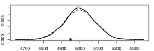
(a) $g(x)=\sum_{i}x_{i}$

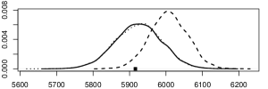
(b) $g(x)=\sum_{i,j:\text{vertical adjacent sites}}I(x_{i}=x_{j})$

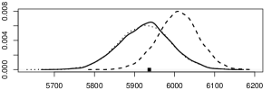
(c) $g(x)=\sum_{i,j:\text{horizontal adjacent sites}}I(x_{i}=x_{j})$

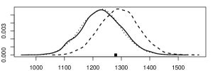
(d) $g(x)=\sum_{\Lambda\in\mathcal{L}_{m}}I\left(x_{\Lambda}={\left[\scriptsize\begin{array}[]{@{}c@{}c@{}}0&0\\ 0&0\end{array}\right]}\right)$

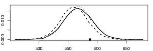
(e) $g(x)=\sum_{\Lambda\in\mathcal{L}_{m}}I\left(x_{\Lambda}={\left[\scriptsize\begin{array}[]{@{}c@{}c@{}}0&1\\ 1&0\end{array}\right]}\right)$

(f) $g(x)=\sum_{\Lambda\in\mathcal{L}_{m}}I\left(x_{\Lambda}={\left[\scriptsize\begin{array}[]{@{}c@{}c@{}}1&1\\ 1&0\end{array}\right]}\right)$

(g) $g(x)=\sum_{i}x_{i}$

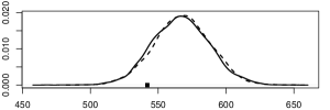
(h) $g(x)=\sum_{\Lambda\in\mathcal{L}_{m}}I\left(x_{\Lambda}={\left[\scriptsize\begin{array}[]{@{}c@{}c@{}}1&1\\ 1&0\end{array}\right]}\right)$

Figure 3: Ising model example: (a)-(f) Distribution of six statistics of realisations from our $2\times 2$ model with posterior samples of $z$ (solid), the Ising model with correct parameter value (dashed), and the Ising model with posterior samples of the parameter value (dotted). In (g) and (h) we compare two of these statistics with results obtained using the exchange algorithm with MCMC samples as auxiliary variables (dashed) instead of the approximation. The data evaluated with each statistic is shown with a black dot.

To study the properties of the MRF $p(\cdot|z)$ when $z$ is a sample from the posterior $p(z|x)$ we take $5000$ samples from the MCMC run for $p(z|x)$ and generate for each of these a corresponding realisation from the MRF $p(\cdot|z)$. To analyse these $5000$ images we use six statistics describing local properties of the images. The statistics used and resulting density estimates (solid) of the distribution of these statistics are shown in Figures 3 (a)-(f).

Figure 3 approximately here.

In the same figures we also show density estimates of the same statistics when images are generated from the Ising model with the true parameter value (dashed), and when images are generated from the Ising model with parameter value $\omega$ generated from the posterior distribution given our observed image $x$ (dotted). In this last case, a zero mean Gaussian prior with standard deviation equal to ten is used for $\omega$. In these figures we also see that the data we use for posterior sampling (black dots) of $z$ is a realisation from the Ising model with low values for the number of equal horizontal and vertical adjacent sites, see Figure 3(b) and 3(c), which causes, as already observed above, our simulations of the second order interactions between horizontal and vertical adjacent sites to be somewhat lower than the true values. In fact we can see that the simulations from the Ising model using posterior samples for the parameter value closely follows that of our $2\times 2$ model. This means that the results from our model is as accurate as the result one gets when knowing that the true model is the Ising model without knowing the model parameter.

To evaluate the quality of the POMM approximation in this example, we also simulate from the posterior distribution with the same RJMCMC algorithm using the approximate exchange algorithm of Murray et al., (2006), as discussed in Section 4.1. We compare in Figures 3 (g) and (h) the results using the POMM approximation (solid) to the results from the approximate exchange algorithm (dashed) using two of our six statistics. We observe that the differences are minimal for these two, and indeed we get as accurate results for the four other statistics as well. That these two very different approximation strategies produces essentially the same results strongly indicate that both procedures are very accurate.

All the above results are for $\gamma=0.5$, but as mentioned in the introduction of this section we also investigate the results for $\gamma=0$ and $1$. For $\gamma=0$ the configuration sets are organised into 3 (66%), 4 (31%) or 5 (3%) groups, and for $\gamma=1$ we get 3 (96%) or 4 (4%) groups. From these numbers we see the effect of varying $\gamma$. In particular when increasing $\gamma$ from $0.5$ to $1.0$ the tendency to group more configuration sets together becomes stronger for this data set.

5.2 Red deer census count data

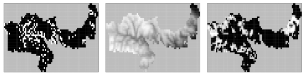
Figure 4: Red deer example: The presence/absence of red deer (left), altitude (middle), and mires (right) in the Grampians Region of north-east Scotland.

In this section we analyse a data set of census counts of red deer in the Grampians Region of north-east Scotland. A full description of the data set is found in Augustin et al., (1996) and Buckland and Elston, (1993). The data is obtained by dividing the region of interest into $n=1277$ grid cells on a lattice and observing the presence or absence of red deer in each cell. In our notation this is our observed image $x$, but in this example we also have the four covariates altitude, mires, north coordinate and east coordinate available in each grid cell. The binary data $x$ and the two first covariates are shown in Figure 4.

Figure 4 approximately here.

We denote the covariate $k$ at a location $(i,j)$ by $y_{i,j,k},\ j=1,2,3,4$, and model them into the likelihood function in the following way

$$p(x|z,\theta^{C},y)=Z\exp{\left(\sum_{\Lambda\in\mathcal{L}_{m}}V_{\Lambda}(x_{\Lambda}|z)+\sum_{(i,j)\in S}x_{i,j}\sum_{k=1}^{4}\theta^{C}_{k}y_{i,j,k}\right)},$$ (45)

where $\theta^{C}=(\theta^{C}_{1},...,\theta^{C}_{4})$ are the parameters for the covariates.

We put independent zero mean Gaussian prior distributions with standard deviation equal to 10 on $\theta^{C}_{j}$, $j=1,...,4$. In the sampling algorithm these covariates are updated using random walk, i.e. we uniformly choose one of the four covariates to update and propose a new value using a Gaussian distribution with the old parameter value as the mean and a standard deviation of $0.1$.

We ran our algorithm for 50000 iterations, and the acceptance rates for the parameter random walk proposal is 42%, the group changing proposal is 33%, the trans-dimensional proposal is 5%, and the covariate proposal is 48%. The posterior most probable grouping becomes $\{c^{0}\}$, $\{c^{1},c^{11},c^{\scriptsize\begin{array}[]{@{}c@{}}1\\ 1\end{array}},c^{\scriptsize\begin{array}[]{@{}c@{}c@{}}1&\\ &1\end{array}},c^{\scriptsize\begin{array}[]{@{}c@{}c@{}}&1\\ 1&\end{array}},c^{\scriptsize\begin{array}[]{@{}c@{}c@{}}1&1\\ 1&\end{array}},c^{\scriptsize\begin{array}[]{@{}c@{}c@{}}1&1\\ &1\end{array}},c^{\scriptsize\begin{array}[]{@{}c@{}c@{}}1&\\ 1&1\end{array}},c^{\scriptsize\begin{array}[]{@{}c@{}c@{}}&1\\ 1&1\end{array}}\}$ and $\{c^{\scriptsize\begin{array}[]{@{}c@{}c@{}}1&1\\ 1&1\end{array}}\}$ with probability 33.2%. In total more than 2500 different groupings are visited, and except for the posterior most probable grouping the posterior probabilities of all other groupings are less than 5%. The estimated posterior probability distribution for the number of groups becomes 43% for 3 groups, 48% for 4 groups, 8% for 5 groups and 1% for 6 groups. In particular, the realisations with four or more groups are mostly groupings where the set $\{c^{1},c^{11},c^{\scriptsize\begin{array}[]{@{}c@{}}1\\ 1\end{array}},c^{\scriptsize\begin{array}[]{@{}c@{}c@{}}1&\\ &1\end{array}},c^{\scriptsize\begin{array}[]{@{}c@{}c@{}}&1\\ 1&\end{array}},c^{\scriptsize\begin{array}[]{@{}c@{}c@{}}1&1\\ 1&\end{array}},c^{\scriptsize\begin{array}[]{@{}c@{}c@{}}1&1\\ &1\end{array}},c^{\scriptsize\begin{array}[]{@{}c@{}c@{}}1&\\ 1&1\end{array}},c^{\scriptsize\begin{array}[]{@{}c@{}c@{}}&1\\ 1&1\end{array}}\}$ is split in various ways. This can also be seen in Figure 5, which shows the estimated posterior probability of two configuration sets being assigned to the same group.

Figure 5 approximately here.

The grey blocks in this figure show the estimated posterior most probable grouping described above. Next we estimate the posterior density for the interaction parameters, see Figure 6.

Figure 6 approximately here.

As we can see, most of the higher order interaction parameters becomes significantly different from zero, suggesting that a $2\times 2$ clique system is needed for this data set. Figure 7 shows the estimated posterior density for the covariate parameters.

Figure 7 approximately here.

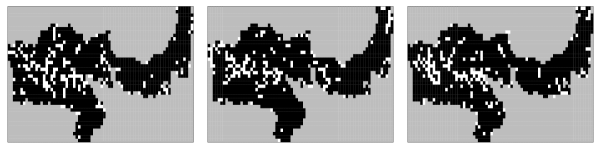
Figure 8: Red deer example: Three realisations from the likelihood for three random samples of $z$ from the posterior distribution.

As we can see from the credibility intervals, all these parameters are significantly different from zero, which justifies the need to include them. Simulations of $p(x|z,\theta^{C},y)$ for three randomly chosen posterior samples of $z$ and $\theta^{C}$ are shown in Figure 8.

Figure 8 approximately here.

As we can see the spatial dependency in these realisations looks similar to the data which indicates that the features of this data set are captured with this model.

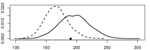
(a) $g(x)=\sum_{i}x_{i}$

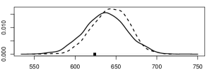
(b) $g(x)=\sum_{i,j:\text{vertical adjacent sites}}I(x_{i}=x_{j})$

(c) $g(x)=\sum_{i,j:\text{horizontal adjacent sites}}I(x_{i}=x_{j})$

(d) $g(x)=\sum_{\Lambda\in\mathcal{L}_{m}}I\left(x_{\Lambda}={\left[\scriptsize\begin{array}[]{@{}c@{}c@{}}0&0\\ 0&0\end{array}\right]}\right)$

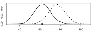
(e) $g(x)=\sum_{\Lambda\in\mathcal{L}_{m}}I\left(x_{\Lambda}={\left[\scriptsize\begin{array}[]{@{}c@{}c@{}}0&1\\ 1&0\end{array}\right]}\right)$

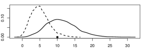
(f) $g(x)=\sum_{\Lambda\in\mathcal{L}_{m}}I\left(x_{\Lambda}={\left[\scriptsize\begin{array}[]{@{}c@{}c@{}}1&1\\ 1&0\end{array}\right]}\right)$

Figure 9: Red deer example: Distribution of six statistics of realisations from our $2\times 2$ model with posterior samples of $z$ (solid), and the nearest neighbour pairwise interaction model (dashed). The data evaluated with each statistic is shown with a black dot.

As discussed above, the estimated marginal posterior densities for the interaction parameters in Figure 6 indicate that higher order interaction parameters are needed for this data set. To investigate this further we also run a corresponding MCMC simulation with a prior where the spatial interaction is as in the nearest neighbour autologistic model defined in Besag, (1972), whereas the covariates are included as in (45). This pairwise interaction prior has three interaction parameters, for first-order interactions and for horisontal and vertical second-order interactions, respectively, and apriori we assume these three parameters to be independent and Gaussian distributed with zero-mean and standard deviations equal to ten. To simulate these three parameters we randomly choose one and propose a zero mean Gaussian change with standard deviation equal to 0.3 to the chosen parameter. For the $\theta_{j}^{C}$ parameters we adopt the same prior and proposals as before. For the pairwise interaction prior and our original prior in (45), Figure 9 shows

Figure 9 approximately here.

estimates of the resulting marginal posterior distributions for the same six statistics studied in our Ising simulation example. For several of the statistics we see that there is a clear difference between the results for the two priors. The differences for the higher-order interaction statistics are perhaps less surprising, but one should note that the distribution of the first-order statistic in Figure 9(a) also changes quite much when allowing higher order interactions. One should also note that our $2\times 2$ model fits better to the statistics of the data, shown as black dots in the figures.

Returning to the $2\times 2$ prior, using $\gamma=0$ in the prior for this data set gives the estimated posterior probability distribution 24%, 63%, 11% and 2% for 3, 4, 5 and 6 groups respectively, whereas for $\gamma=1$ we obtain 60%, 35% and 5% for 3, 4 and 5 groups respectively. Again we see that higher values of $\gamma$ results in more realisations with fewer number of groups. However, for all the three values of $\gamma$ the estimated most probable grouping is the same.

We end our discussion of this data set by mentioning that some results when assuming a clique size of $3\times 3$ is included in the supplementary material of this paper. These results indicate that no more significant structure is introduced in the $3\times 3$ case for this data set.

6 Closing remarks

Our main focus in this paper is to design a generic prior distribution for the parameters of an MRF. This is done by assuming a set of maximal cliques defined from a template maximal clique $\Lambda_{0}$, but as the number of free parameters grows quickly as a function of the number of elements in $\Lambda_{0}$ we construct our prior distribution such that it gives a positive probability for groups of parameters to have exactly the same value. In that way we reduce the effective number of parameters, still keeping the flexibility large cliques provides. Proposal distributions that enable us to simulate from the resulting posterior distributed is also presented. However, to evaluate the likelihood we use a previously defined approximation to MRFs (Austad, 2011), and the trade off between accuracy and computational complexity limits in practice the size of the cliques that can be assumed. An alternative to approximations is perfect sampling (Propp and Wilson, 1996), but this was in all our examples too computationally intensive. A third alternative would be to use an MCMC sample of $x$ instead of a perfect sample, as described in for instance Everitt, (2012). An issue with this approach is the need to set a burn in period for the sampler of $x$, where a too long burn in period would make the parameter sampler too intensive. Lastly, we illustrate the effect of our prior distribution and sampling algorithm on two examples.

Our focus in this paper is on binary MRFs. It is however possible to generalise our framework to discrete MRFs, i.e. where $x_{i}\in\{0,1,...,K\}$ for $K\geq 2$. An identifiable parametrisation of a discrete MRF using clique potentials can with a small effort be defined in a similar way to what is done in the binary case, and ones this parametrisation is established, the prior distribution presented in this paper can be used unchanged. The same apply to our sampling strategy.

With our prior distribution the size of the maximal cliques, and thereby the number of configuration sets, act as a hyper parameter and must be set prior to any sampling algorithm. One could imagine putting a prior also on $\Lambda_{0}$, introducing the need to construct algorithms for trans-dimensional sampling also for $\Lambda_{0}$. Another way to avoid the need to set the number of configuration sets would be to construct a prior distribution for the $\beta$ parameters. A natural choice would be to construct a positive prior probability for these parameters to be exactly zero, and in this way the significant interactions of an MRF can be inferred from data. However, as discussed above, it is not clear to us how to design generic prior distributions for the values of these interaction parameters, as higher order interactions intuitively would be different from lower order interaction. Also, grouping $\beta$ parameters together in order to reduce the number of parameters would, for the same reason as above, make little sense. An ideal solution would be somehow to draw strength from both of the two parametrisations in order to assign a prior distribution to both the appearance of different cliques and the number of free parameters. This idea is currently work in progress.

Supporting Information

Additional Supporting Information may be found in the online version of this article:

Section S.1: Proof of one-to-one relation between $\phi$ and $\beta$.

Section S.2: Proof of translational invariance for $\beta$.

Section S.3: Proof of translational invariance for $\phi$.

Section S.4: Details for the MCMC sampling algorithm.

Section S.5: The independence model with check of convergence.

Section S.6: Reed deer data with $3\times 3$ maximal cliques.

Section S.7: Parallelisation of the sampling algorithm.

Petter Arnesen, Department of Mathematical Sciences, Norwegian University of Science and Technology, Trondheim 7491, Norway.
E-mail: petterar@math.ntnu.no

$k\times l$	$2^{kl}$	$N_{\Lambda_{0}}$
$1\times 2$	4	2
$2\times 2$	16	10
$2\times 3$	64	44
$3\times 3$	512	400
$3\times 4$	4096	3392
$4\times 4$	65536	57856

Table 1: The number of configurations and the corresponding number of free parameters $N_{\Lambda_{0}}$ when $\Lambda_{0}$ is a $k\times l$ block of nodes.

$$\begin{array}[]{cccccccccccc}c^{0}&\pagecolor{gray!25}1.00&\pagecolor{gray!25}1.00&&&&&&&&&\\ c^{\scriptsize\begin{array}[]{@{}c@{}c@{}}1&1\\ 1&1\end{array}}&\pagecolor{gray!25}1.00&\pagecolor{gray!25}1.00&&&&&&&&&\\ c^{1}&&&\pagecolor{gray!25}1.00&\pagecolor{gray!25}0.96&\pagecolor{gray!25}0.97&\pagecolor{gray!25}0.97&\pagecolor{gray!25}0.97&\pagecolor{gray!25}0.97&\pagecolor{gray!25}0.96&&\\ c^{11}&&&\pagecolor{gray!25}0.96&\pagecolor{gray!25}1.00&\pagecolor{gray!25}0.96&\pagecolor{gray!25}0.96&\pagecolor{gray!25}0.96&\pagecolor{gray!25}0.96&\pagecolor{gray!25}0.96&&\\ c^{\scriptsize\begin{array}[]{@{}c@{}}1\\ 1\end{array}}&&&\pagecolor{gray!25}0.97&\pagecolor{gray!25}0.96&\pagecolor{gray!25}1.00&\pagecolor{gray!25}0.97&\pagecolor{gray!25}0.96&\pagecolor{gray!25}0.96&\pagecolor{gray!25}0.95&&\\ c^{\scriptsize\begin{array}[]{@{}c@{}c@{}}1&1\\ 1&\end{array}}&&&\pagecolor{gray!25}0.97&\pagecolor{gray!25}0.96&\pagecolor{gray!25}0.97&\pagecolor{gray!25}1.00&\pagecolor{gray!25}0.96&\pagecolor{gray!25}0.96&\pagecolor{gray!25}0.96&&\\ c^{\scriptsize\begin{array}[]{@{}c@{}c@{}}1&1\\ &1\end{array}}&&&\pagecolor{gray!25}0.97&\pagecolor{gray!25}0.96&\pagecolor{gray!25}0.96&\pagecolor{gray!25}0.96&\pagecolor{gray!25}1.00&\pagecolor{gray!25}0.97&\pagecolor{gray!25}0.97&&\\ c^{\scriptsize\begin{array}[]{@{}c@{}c@{}}1&\\ 1&1\end{array}}&&&\pagecolor{gray!25}0.97&\pagecolor{gray!25}0.96&\pagecolor{gray!25}0.96&\pagecolor{gray!25}0.96&\pagecolor{gray!25}0.97&\pagecolor{gray!25}1.00&\pagecolor{gray!25}0.96&&\\ c^{\scriptsize\begin{array}[]{@{}c@{}c@{}}&1\\ 1&1\end{array}}&&&\pagecolor{gray!25}0.96&\pagecolor{gray!25}0.96&\pagecolor{gray!25}0.95&\pagecolor{gray!25}0.96&\pagecolor{gray!25}0.97&\pagecolor{gray!25}0.96&\pagecolor{gray!25}1.00&&\\ c^{\scriptsize\begin{array}[]{@{}c@{}c@{}}1&\\ &1\end{array}}&&&&&&&&&&\pagecolor{gray!25}1.00&\pagecolor{gray!25}1.00\\ c^{\scriptsize\begin{array}[]{@{}c@{}c@{}}&1\\ 1&\end{array}}&&&&&&&&&&\pagecolor{gray!25}1.00&\pagecolor{gray!25}1.00\\ &c^{0}&c^{\scriptsize\begin{array}[]{@{}c@{}c@{}}1&1\\ 1&1\end{array}}&c^{1}&c^{11}&c^{\scriptsize\begin{array}[]{@{}c@{}}1\\ 1\end{array}}&c^{\scriptsize\begin{array}[]{@{}c@{}c@{}}1&1\\ 1&\end{array}}&c^{\scriptsize\begin{array}[]{@{}c@{}c@{}}1&1\\ &1\end{array}}&c^{\scriptsize\begin{array}[]{@{}c@{}c@{}}1&\\ 1&1\end{array}}&c^{\scriptsize\begin{array}[]{@{}c@{}c@{}}&1\\ 1&1\end{array}}&c^{\scriptsize\begin{array}[]{@{}c@{}c@{}}1&\\ &1\end{array}}&c^{\scriptsize\begin{array}[]{@{}c@{}c@{}}&1\\ 1&\end{array}}\end{array}$$

Figure 1: Ising model example: Estimated posterior probabilities for two configuration sets to be grouped together. The true grouping is shown in grey, and only probabilities larger than $5\%$ are given. Note the permutation done to the ordering of the configuration sets $c_{i}$.

(a) $\beta^{\scriptsize\begin{array}[]{@{}l@{}l@{}}&\\ \framebox(5.0,5.0)[]{}&\end{array}}\ (-1.62,-1.38)$

(b) $\beta^{\scriptsize\begin{array}[]{@{}l@{}l@{}}\framebox(5.0,5.0)[]{}&\framebox(5.0,5.0)[]{}\\ &\end{array}}\ (0.69,0.81)$

(c) $\beta^{\scriptsize\begin{array}[]{@{}l@{}l@{}}\framebox(5.0,5.0)[]{}&\\ \framebox(5.0,5.0)[]{}&\end{array}}\ (0.69,0.81)$

(d) $\beta^{\scriptsize\begin{array}[]{@{}l@{}l@{}}\framebox(5.0,5.0)[]{}&\\ &\framebox(5.0,5.0)[]{}\end{array}}\ (-0.09,0.09)$

(e) $\beta^{\scriptsize\begin{array}[]{@{}l@{}l@{}}&\framebox(5.0,5.0)[]{}\\ \framebox(5.0,5.0)[]{}&\end{array}}\ (-0.09,0.09)$

(f) $\beta^{\scriptsize\begin{array}[]{@{}l@{}l@{}}\framebox(5.0,5.0)[]{}&\framebox(5.0,5.0)[]{}\\ \framebox(5.0,5.0)[]{}&\end{array}}\ (-0.10,0.08)$

(g) $\beta^{\scriptsize\begin{array}[]{@{}l@{}l@{}}\framebox(5.0,5.0)[]{}&\framebox(5.0,5.0)[]{}\\ &\framebox(5.0,5.0)[]{}\end{array}}\ (-0.09,0.09)$

(h) $\beta^{\scriptsize\begin{array}[]{@{}l@{}l@{}}\framebox(5.0,5.0)[]{}&\\ \framebox(5.0,5.0)[]{}&\framebox(5.0,5.0)[]{}\end{array}}\ (-0.10,0.09)$

(i) $\beta^{\scriptsize\begin{array}[]{@{}l@{}l@{}}&\framebox(5.0,5.0)[]{}\\ \framebox(5.0,5.0)[]{}&\framebox(5.0,5.0)[]{}\end{array}}\ (-0.09,0.09)$

(j) $\beta^{\scriptsize\begin{array}[]{@{}l@{}l@{}}\framebox(5.0,5.0)[]{}&\framebox(5.0,5.0)[]{}\\ \framebox(5.0,5.0)[]{}&\framebox(5.0,5.0)[]{}\end{array}}\ (-0.17,0.19)$

Figure 2: Ising model example: Estimated marginal posterior distribution for the interaction parameters. True values are shown with a black dot and estimated 95% credibility intervals are given for each parameter.

$$\begin{array}[]{cccccccccccc}c^{0}&\pagecolor{gray!25}1.00&&&&&0.12&0.06&&&&\\ c^{1}&&\pagecolor{gray!25}1.00&\pagecolor{gray!25}0.69&\pagecolor{gray!25}0.68&\pagecolor{gray!25}0.58&\pagecolor{gray!25}0.67&\pagecolor{gray!25}0.75&\pagecolor{gray!25}0.70&\pagecolor{gray!25}0.68&\pagecolor{gray!25}0.60&\\ c^{11}&&\pagecolor{gray!25}0.69&\pagecolor{gray!25}1.00&\pagecolor{gray!25}0.80&\pagecolor{gray!25}0.69&\pagecolor{gray!25}0.62&\pagecolor{gray!25}0.64&\pagecolor{gray!25}0.70&\pagecolor{gray!25}0.69&\pagecolor{gray!25}0.65&\\ c^{\scriptsize\begin{array}[]{@{}c@{}}1\\ 1\end{array}}&&\pagecolor{gray!25}0.68&\pagecolor{gray!25}0.80&\pagecolor{gray!25}1.00&\pagecolor{gray!25}0.69&\pagecolor{gray!25}0.61&\pagecolor{gray!25}0.64&\pagecolor{gray!25}0.70&\pagecolor{gray!25}0.69&\pagecolor{gray!25}0.65&\\ c^{\scriptsize\begin{array}[]{@{}c@{}c@{}}1&\\ &1\end{array}}&&\pagecolor{gray!25}0.58&\pagecolor{gray!25}0.69&\pagecolor{gray!25}0.69&\pagecolor{gray!25}1.00&\pagecolor{gray!25}0.55&\pagecolor{gray!25}0.58&\pagecolor{gray!25}0.64&\pagecolor{gray!25}0.64&\pagecolor{gray!25}0.69&0.05\\ c^{\scriptsize\begin{array}[]{@{}c@{}c@{}}&1\\ 1&\end{array}}&0.12&\pagecolor{gray!25}0.67&\pagecolor{gray!25}0.62&\pagecolor{gray!25}0.61&\pagecolor{gray!25}0.55&\pagecolor{gray!25}1.00&\pagecolor{gray!25}0.62&\pagecolor{gray!25}0.61&\pagecolor{gray!25}0.61&\pagecolor{gray!25}0.57&\\ c^{\scriptsize\begin{array}[]{@{}c@{}c@{}}1&1\\ 1&\end{array}}&0.06&\pagecolor{gray!25}0.75&\pagecolor{gray!25}0.64&\pagecolor{gray!25}0.64&\pagecolor{gray!25}0.58&\pagecolor{gray!25}0.62&\pagecolor{gray!25}1.00&\pagecolor{gray!25}0.65&\pagecolor{gray!25}0.64&\pagecolor{gray!25}0.58&\\ c^{\scriptsize\begin{array}[]{@{}c@{}c@{}}1&1\\ &1\end{array}}&&\pagecolor{gray!25}0.70&\pagecolor{gray!25}0.70&\pagecolor{gray!25}0.70&\pagecolor{gray!25}0.64&\pagecolor{gray!25}0.61&\pagecolor{gray!25}0.65&\pagecolor{gray!25}1.00&\pagecolor{gray!25}0.67&\pagecolor{gray!25}0.63&\\ c^{\scriptsize\begin{array}[]{@{}c@{}c@{}}1&\\ 1&1\end{array}}&&\pagecolor{gray!25}0.68&\pagecolor{gray!25}0.69&\pagecolor{gray!25}0.69&\pagecolor{gray!25}0.64&\pagecolor{gray!25}61&\pagecolor{gray!25}0.64&\pagecolor{gray!25}0.67&\pagecolor{gray!25}1.00&\pagecolor{gray!25}0.63&\\ c^{\scriptsize\begin{array}[]{@{}c@{}c@{}}&1\\ 1&1\end{array}}&&\pagecolor{gray!25}0.60&\pagecolor{gray!25}0.65&\pagecolor{gray!25}0.65&\pagecolor{gray!25}0.69&\pagecolor{gray!25}0.57&\pagecolor{gray!25}0.58&\pagecolor{gray!25}0.63&\pagecolor{gray!25}0.63&\pagecolor{gray!25}1.00&0.06\\ c^{\scriptsize\begin{array}[]{@{}c@{}c@{}}1&1\\ 1&1\end{array}}&&&&&0.05&&&&&0.06&\pagecolor{gray!25}1.00\\ &c^{0}&c^{1}&c^{11}&c^{\scriptsize\begin{array}[]{@{}c@{}}1\\ 1\end{array}}&c^{\scriptsize\begin{array}[]{@{}c@{}c@{}}1&\\ &1\end{array}}&c^{\scriptsize\begin{array}[]{@{}c@{}c@{}}&1\\ 1&\end{array}}&c^{\scriptsize\begin{array}[]{@{}c@{}c@{}}1&1\\ 1&\end{array}}&c^{\scriptsize\begin{array}[]{@{}c@{}c@{}}1&1\\ &1\end{array}}&c^{\scriptsize\begin{array}[]{@{}c@{}c@{}}1&\\ 1&1\end{array}}&c^{\scriptsize\begin{array}[]{@{}c@{}c@{}}&1\\ 1&1\end{array}}&c^{\scriptsize\begin{array}[]{@{}c@{}c@{}}1&1\\ 1&1\end{array}}\end{array}$$

Figure 5: Red deer example: Estimated posterior probabilities for two configuration sets to be grouped together. The estimated most probable grouping is shown in grey, and only probabilities larger than 5 % are given.

(a) $\beta^{\scriptsize\begin{array}[]{@{}l@{}l@{}}&\\ \framebox(5.0,5.0)[]{}&\end{array}}\ (-3.52,-2.85)$

(b) $\beta^{\scriptsize\begin{array}[]{@{}l@{}l@{}}\framebox(5.0,5.0)[]{}&\framebox(5.0,5.0)[]{}\\ &\end{array}}\ (0.92,1.77)$

(c) $\beta^{\scriptsize\begin{array}[]{@{}l@{}l@{}}\framebox(5.0,5.0)[]{}&\\ \framebox(5.0,5.0)[]{}&\end{array}}\ (0.91,1.77)$

(d) $\beta^{\scriptsize\begin{array}[]{@{}l@{}l@{}}\framebox(5.0,5.0)[]{}&\\ &\framebox(5.0,5.0)[]{}\end{array}}\ (0.62,1.54)$.

(e) $\beta^{\scriptsize\begin{array}[]{@{}l@{}l@{}}&\framebox(5.0,5.0)[]{}\\ \framebox(5.0,5.0)[]{}&\end{array}}\ (0.14,0.88)$

(f) $\beta^{\scriptsize\begin{array}[]{@{}l@{}l@{}}\framebox(5.0,5.0)[]{}&\framebox(5.0,5.0)[]{}\\ \framebox(5.0,5.0)[]{}&\end{array}}\ (-1.08,-0.09)$

(g) $\beta^{\scriptsize\begin{array}[]{@{}l@{}l@{}}\framebox(5.0,5.0)[]{}&\framebox(5.0,5.0)[]{}\\ &\framebox(5.0,5.0)[]{}\end{array}}\ (-1.54,-0.25)$

(h) $\beta^{\scriptsize\begin{array}[]{@{}l@{}l@{}}\framebox(5.0,5.0)[]{}&\\ \framebox(5.0,5.0)[]{}&\framebox(5.0,5.0)[]{}\end{array}}\ (-1.55,-0.28)$

(i) $\beta^{\scriptsize\begin{array}[]{@{}l@{}l@{}}&\framebox(5.0,5.0)[]{}\\ \framebox(5.0,5.0)[]{}&\framebox(5.0,5.0)[]{}\end{array}}\ (-0.88,0.47)$

(j) $\beta^{\scriptsize\begin{array}[]{@{}l@{}l@{}}\framebox(5.0,5.0)[]{}&\framebox(5.0,5.0)[]{}\\ \framebox(5.0,5.0)[]{}&\framebox(5.0,5.0)[]{}\end{array}}\ (-3.70,0.29)$

Figure 6: Red deer example: Estimated marginal posterior distribution for the interaction parameters. Estimated 95% credibility interval is given for each parameter.

(a) $\theta^{C}_{1}\ (-0.50,-0.21)$

(b) $\theta^{C}_{2}\ (-0.36,-0.07)$

(c) $\theta^{C}_{3}\ (-0.55,-0.27)$

(d) $\theta^{C}_{4}\ (-0.26,-0.05)$

Figure 7: Red deer example: Estimated marginal posterior distributions for the parameters of the covariates. Estimated 95 % credibility interval is given for each parameter.

References

- Augustin et al., (1996) Augustin, N. H., Mugglestone, M. A., and Buckland, S. T. (1996). “An autologistic model for the spatial distribution of wildlife.” Journal of Applied Ecology, 33, 339–347.
- Austad, (2011) Austad, H. M. (2011). “Approximations of binary Markov random fields.” Ph.D. thesis, Norwegian University of Science and Technology. Thesis number 292:2011. Available from http://urn.kb.se/resolve?urn=urn:nbn:no:ntnu:diva-14922.
- Besag, (1974) Besag, J. (1974). “Spatial interaction and the statistical analysis of lattice systems.” Journal of the Royal Statistical Society. Series B (Methodological), 36, 2, 192–236.
- Besag, (1986) — (1986). “On the statistic analysis of dirty pictures.” Journal of the Royal Statistical Society. Series B (Methodological), 48, 259–302.
- Besag, (1972) Besag, J. E. (1972). “Nearest-neighbour systems and the auto-logistic model for binary data.” Journal of the Royal Statistical Society, Series B, 34, 75–83.
- Bishop et al., (1975) Bishop, Y. M. M., Fienberg, S. E., and Holland, P. W. (1975). Discrete Multivariate Analysis. Cambridge: MA: MIT Press.
- Buckland and Elston, (1993) Buckland, S. T. and Elston, D. A. (1993). “Empirical models for the spatial distribution of wildlife.” Journal of Applied Ecology, 30, 478–495.
- Caimo and Friel, (2011) Caimo, A. and Friel, N. (2011). “Bayesian inference for exponential random graph models.” Social Networks, 33, 41–55.
- Clifford, (1990) Clifford, P. (1990). “Markov random fields in statistics.” In Disorder in Physical Systems, A Volume in Honour of John M.Hammersley, eds. G. Grimmett and D. J. Welsh. Oxford University Press.
- Cressie and Davidson, (1998) Cressie, N. and Davidson, J. (1998). “Image analysis with partially ordered Markov models.” Computational Statistics and Data Analysis, 29, 1–26.
- Cressie, (1993) Cressie, N. A. (1993). Statistics for Spatial Data. 2nd ed. New York: John Wiley.
- Dellaportas and Forster, (1999) Dellaportas, P. and Forster, J. J. (1999). “Markov chain Monte Carlo model determination for hierarchical and graphical log-linear models.” Biometrika, 86, 615–633.
- Descombes et al., (1995) Descombes, X., Mangin, J., Pechersky, E., and Sigelle, M. (1995). “Fine structures preserving Markov model for image processing.” In Proc. 9th SCIA 95, Uppsala, Sweden, 349–356.
- Diaconis and Freedman, (1980) Diaconis, P. and Freedman, D. (1980). “Finite exchangeable sequences.” The Annals of Probability, 8, 639–859.
- Everitt, (2012) Everitt, R. G. (2012). “Bayesian parameter estimation for latent Markov random fields and social networks.” Journal of Computational and Graphical Statistics, 21, 940–960.
- Friel et al., (2009) Friel, N., Pettitt, A. N., Reeves, R., and Wit, E. (2009). “Bayesian inference in hidden Markov random fields for binary data defined on large lattices.” Journal of Computational and Graphical Statistics, 18, 243–261.
- Grabisch et al., (2000) Grabisch, M., Marichal, L.-L., and Roubens, M. (2000). “Equivalent representation of set function.” Mathematics of Operations Reasearch, 25, 157–178.
- Green, (1995) Green, P. J. (1995). “Reversible jump MCMC computation and Bayesian model determination.” Biometrika, 82, 711–732.
- Hammer and Holzman, (1992) Hammer, P. and Holzman, R. (1992). “Approximations of pseudo-boolean functions; application to game theory.” Methods and Models of Operations Research, 36, 3–21.
- Heikkinen and Högmander, (1994) Heikkinen, J. and Högmander, H. (1994). “Fully Bayesian approach to image restoration with an application in biogeography.” Applied Statistics, 43, 569–582.
- Higdon et al., (1997) Higdon, D. M., Bowsher, J. E., Johnsen, V. E., Turkington, T. G., Gilland, D. R., and Jaszczak, R. J. (1997). “Fully Bayesian estimation of Gibbs hyperparameters for emission computed tomography data.” IEEE Transactions on medical imaging, 16, 516–526.
- Hurn et al., (2003) Hurn, M., Husby, O., and Rue, H. (2003). “A tutorial on image analysis.” In Spatial Statistics and Computational Methods, ed. J. Møller, vol. 173 of Lecture Notes in Statistics, 87–141. Springer Verlag.
- Martins et al., (2013) Martins, T. G., Simpson, D., Lindgren, F., and Rue, H. (2013). “Bayesian computing with INLA: new features.” Computational Statistics and Data Analysis, 67, 68–83.
- Massam et al., (2009) Massam, H., Liu, J., and Dobra, A. (2009). “A conjugate prior for discrete hierarchical log-linear models.” The Annals of Statistics, 37, 3431–3467.
- McGrory et al., (2012) McGrory, C. A., Pettitt, A. N., Reeves, R., Griffin, M., and Dwyer, M. (2012). “Variational Bayes and the reduced dependence approximation for the autologistic model on an irregular grid with applications.” Journal of Computational and Graphical Statistics, 21, 781–796.
- Møller et al., (2006) Møller, J., Pettitt, A., Reeves, R., and Berthelsen, K. (2006). “An efficient Markov chain Monte Carlo method for distributions with intractable normalising constants.” Biometrika, 93, 451–458.
- Murray et al., (2006) Murray, I., Ghahramani, Z., and MacKay, D. (2006). “MCMC for doubly-intractable distributions.” In Proceedings of the Twenty-Second Conference Annual Conference on Uncertainty in Artificial Intelligence (UAI-06), 359–366. Arlington, Virginia: AUAI Press.
- Overstall and King, (2014) Overstall, A. and King, R. (2014). “A default prior distribution for contingency tables with correlated factor levels.” Statistical Methodology, 16, 90–99.
- Propp and Wilson, (1996) Propp, J. G. and Wilson, D. B. (1996). “Exact sampling with coupled Markov chains and applications to statistical mechanics.” Random Structures & Algorithms, 9, 223–252.
- Ronald L. Graham, (1988) Ronald L. Graham, Donald E. Knuth, O. P. (1988). Concrete Mathematics. 2nd ed. Reading MA: Addison-Wesley.
- Rue et al., (2009) Rue, H., Martino, S., and Chopin, N. (2009). “Approximate Bayesian inference for latent Gaussian models by using integrated nested Laplace approximations.” Journal of the Royal Statistical Society, Series B, 71, 319–392.
- Tjelmeland and Austad, (2012) Tjelmeland, H. and Austad, H. M. (2012). “Exact and approximate recursive calculations for binary Markov random fields defined on graphs.” Journal of Computational and Graphical Statistics, 21, 758–780.
- Tjelmeland and Besag, (1998) Tjelmeland, H. and Besag, J. (1998). “Markov Random Fields with Higher Order Interactions.” Scandinavian Journal of Statistics, 25, 415–433.