A Multi-wavelength study of the M dwarf binary YY Geminorum

Abstract

We review the results of the 1988 multi-wavelength campaign on the late-type eclipsing binary YY Geminorum. Observations include: broad-band optical and near infra-red photometry, simultaneous optical and ultraviolet (IUE) spectroscopy, X-ray (Ginga) and radio (VLA) data. From models fitted to the optical light curves, fundamental physical parameters have been determined together with evidence for transient maculations (spots) located near quadrature longitudes and intermediate latitudes.

Eclipses were observed at optical, ultraviolet and radio wavelengths. Significant drops in 6cm radio emission near the phases of both primary and secondary eclipse indicate relatively compact radio emitting volumes that may lie between the binary components. IUE observations during secondary eclipse are indicative of a uniform chromosphere saturated with MgII plage-type emission and an extended volume of Ly$\alpha$ emission.

Profile fitting of high-dispersion H$\alpha$ spectra confirms the chromospheric saturation and indicates significant H$\alpha$ opacity to heights of a few percent of the photospheric radius. There is evidence for an enhanced H$\alpha$ emission region visible near phase 0.25-0.35 which may be associated with a large spot on the primary and with two small optical flares which were also observed at other wavelengths: one in microwave radiation and the other in X-rays. For both flares, L_X/L_opt is consistent with energy release in closed magnetic structures.

1 Introduction

YY Geminorum, (BD +32 1582, SAO 60199, Gliese 278c), is a short period (19.54 hours) eclipsing binary with two almost identical dM1e (flare star) components. The close binary is a subsystem of the nearby Castor multiple star (YY Gem = Castor C), at a distance of $\sim$14.9 pc. The binary nature was discovered in 1916 (Adams & Joy, 1917) and the first spectroscopic orbits were given by Joy & Sanford (1926). As the brightest known eclipsing binary of the dMe type, YY Gem is an important fundamental standard for defining the low-mass Main Sequence mass-luminosity and mass-radius relationships (Torres & Ribas, 2002). However, it was clear already from Kron’s (1952) pioneer study that there are significant surface inhomogeneities (starspots) affecting the observed brightness of both components, likely to complicate data analysis. YY Gem was the first star, after the Sun, in which such maculation effects were demonstrated. Before we can accurately define the intrinsic luminosities of such stars we need to clarify the scale of these effects. This is also significant for comparing the photometric parallax with direct measurements, such as that from HIPPARCOS (Budding et al., 2005).

The system was reviewed by Torres & Ribas (2002) and Qian et al. (2002), the latter concentrating mainly on apparent variations of the orbital period. Torres & Ribas (2002) gave revised values for the mean mass and radius of the very similar components as (solar units) $M$ = 0.5992$\pm$0.0047, $R$ = 0.6191$\pm$0.0057, with mean effective temperature $T$ = 3820$\pm$100 K, as well as an improved parallax for the system of 66.90$\pm$0.63 mas. From such results, Torres & Ribas argued that there had been a tendency to adopt systematically erroneous parameters for dwarf stars comparable to YY Gem, with wider implications for low-mass stars in general.

Determination of the precise structure of these stars, in view of the absence of definitive information on their intrinsic, spot-free, luminosities, is still rather an open question. Torres & Ribas (2002) and Qian et al. (2002) revised the work of Chabrier & Baraffe (1995), giving radiative core radii of about 70%, leaving the outer 30% to account for the convective zone. The strong subsurface convective motions, give rise to large-scale magnetic fields that produce large starspots (cf. Bopp & Evans, 1973). Moffet first reported large flare events, and, in subsequent studies, YY Gem has been shown to be very active (Moffet and Barnes, 1979; Lacy et al., 1976; Doyle & Butler, 1985; Doyle & Mathioudakis, 1990; Doyle et al. 1990).

Doyle et al (1990) have previously described photometric observations of repetitive, apparently periodic, flares on YY Gem which were observed during this programme. More recently, Gao et al. (2008) modelled such periodicity effects on the basis of magnetic reconnection between loops on the two stars generating interbinary flares. Fast magneto-acoustic waves in plasma trapped in the space between the two components are thought to modulate the magnetic reconnection, producing a periodic behaviour of the flaring rate. Doyle et al. (1990) had previously suggested filament oscillations. Several authors, (see Vrsnak et al. 2007) have subsequently reported solar filament oscillations of similar duration to those suggested on YY Gem.

Multi-wavelength observations of flare activity on YY Gem were initiated by Jackson, Kundu & White (1989) using radio data from the VLA (see also, Gary, 1986). Stelzer et al. (2002) used the Chandra and XMM-Newton satellites in simultaneous observations of the X-ray spectrum, while Saar & Bookbinder (2003) carried out far ultraviolet observations. Impulsive UV and X-ray phenomena, taken to be essentially flare-like, were shown to be orders of magnitude stronger than those occurring on the Sun (Haisch et al., 1990). Tsikoudi & Kellett (2000), reviewing X-ray and UV observations of the Castor system, reported a large (EXOSAT) flare event with total X-ray emission estimated as $\sim$7$\pm 1\times 10^{33}$ ergs. Their comparison of X-ray and bolometric heating rates pointed to strong magnetic activity within hot coronal components.

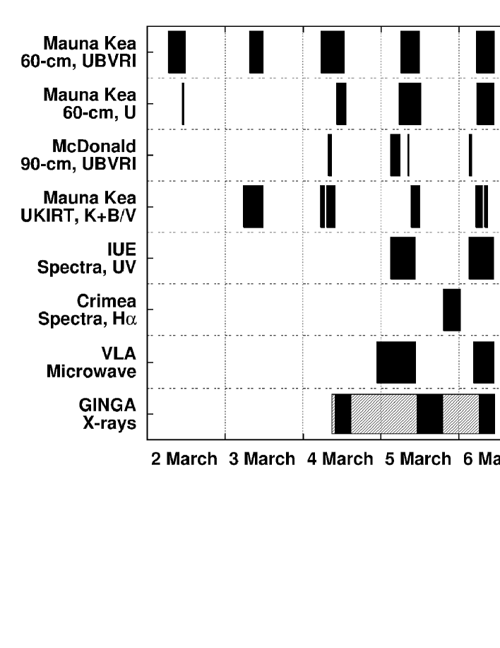
Figure 1: Time-line of various facilities used in the multiwavelength campaign of 1988

Table 1: Multiwavelength Observations of YY Gem, March 1988

Institute	Observer	Facility	Range
ISAS-Tokyo	Bromage	GINGA	ME X-rays
VILSPA-ESA	Foing	IUE	UV
Mauna Kea	Butler	UKIRT	IR
Mauna Kea	Doyle/Butler	0.6m	UBVRI
McDonald Obs.	Frueh	0.9m MCD	UBVRI
JILA Boulder	Brown	VLA	5 & 1.4 GHz
Crimea Obs.	Tuominen	2.6m Shajn	UBVRI + H ${\alpha}$

In this article, we concentrate on the multiwavelength campaign initiated from the Armagh Observatory in 1988 (Butler, 1988). Our general aim is to bring together results of some work, previously reported (e.g. Doyle et al. 1990, Butler, et al. 1994, 1995, Budding et al. 1996, Tuominen et al. 1989) with contemporaneous satellite and radio observations thereby allowing an overview of the campaign. One specific intention concerns the various light curves and their analyses in terms of standard eclipsing binary models that include photospheric inhomogeneities. In addition, we present hitherto unpublished, ultraviolet (IUE), radio (VLA) and X-ray (Ginga) data, which should be relevant to subsequent studies. A number of optical flares were observed but only two of these were seen at other wavelengths, one in X-rays by Ginga and the other in the microwave region by the VLA.

2 The 1988 multi-wavelength campaign on YY Geminorum

In late February to early March 1988, YY Gem was the object of a coordinated multiwavelength campaign to observe the star simultaneously in radio, near infra-red, X-rays, UV and optical radiation (Butler, 1988). The principal objectives of this programme were: (i) To provide multicolour photometry of the light curve in order to establish (a) the distribution of surface inhomogeneities (starspots), and (b) the temperature difference of these inhomogeneous regions from the normal photosphere. (ii) To provide high time-resolution photometry in V and K during the eclipses in order to check on possible surface inhomogeneities by ‘eclipse imaging’ — i.e. examining any small disturbances observed in the light curve during eclipses. (iii) To use optical spectroscopy, X-ray and radio monitoring to probe the outer atmospheres of the components and assess any topographical connection between photospheric spots and bright chromospheric or coronal regions. (iv) To monitor flares on YY Gem in as many separate wavebands as possible in order to check their energy distribution and constrain models.

The programme involved the facilities and observations given in Table 1. Several other organisations offered support to the campaign, but unfortunately a number of these were unable to provide useful data due to poor observing conditions. In Figure 1, we show the overlap between observing facilities that were successful in obtaining data. Seven major facilities provided the most relevant data and six of these were operative on Mar 5 and 6, with a few hours of overlap on those two days; and to a lesser extent on Mar 4.

Figure 2: Hawaii 0.6 m UBVRI light curves of YY Gem.

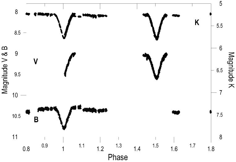
Figure 3: UKIRT-BVK light curves of YY Gem.

3 UBVRIK photometry

3.1 Photometric Techniques

To achieve the photometric aims we required broad-band photometry covering as much of the optical and infra-red regions as possible. We therefore operated two telescopes simultaneously: the University of Hawaii 0.6^m telescope on Mauna Kea and the neighbouring 3.8^m United Kingdom Infra-Red Telescope (UKIRT). Some additional observations were contributed by Marion Frueh of McDonald Observatory, Texas.

All observers were alerted to a particular problem associated with photometry of YY Gem, namely that the close proximity (separation $\sim$71 arcsec) to YY Gem of the bright star Castor (A2 type, V $\sim$1.6) makes it difficult to obtain repeatable and consistent sky background measurements, particularly in the U and B bands, where YY Gem is weak and Castor bright. Kron (1952) commented that, in the vicinity of YY Gem, 30% of the monitored blue light originated with Castor and only 70% with YY Gem itself (Budding & Kitamura 1974). For this campaign, in order to reduce the errors associated with scattered light, observers were requested to take the mean of two adjacent sky areas, one to the east and another to the west of YY Gem. Frequent reference to three nearby comparison stars: BD 32°1577, BD 31°1611 and BD 31°1627, together with standard transformation equations and mean extinction coefficients allowed a photometric accuracy $\sim$ 0.01 magnitudes to be achieved. Lists of the standards used, the colour equations derived and the reduced photometric observations are given in the supplementary electronic tables (http://star.arm.ac.uk/preprints/2014/654/).

3.2 UBVRIK photometry from the 0.6m telescope on Mauna Kea

The UBVRI photometry, from the 0.6^m telescope and Tinsley Photometer, was standardised to the Johnson UBV and Cape/Kron RI systems using equatorial and southern hemisphere standards from Cousins (1980, 1984). The following mean extinction coefficients were adopted: $\kappa_{U}=0.22$, $\kappa_{B}=0.16$, $\kappa_{V}=0.12$, $\kappa_{R}=0.10$ and $\kappa_{I}=0.07$. Due to the manual operation of the Tinsley photoelectric photometer, time-resolution for a single complete UBVRI set of measurements was restricted to several minutes. This was satisfactory for the slower variations associated with eclipse effects and the rotational modulation of spots, but unsuitable for flare monitoring. Therefore, two modes of observation were used on this telescope: (1) UBVRI photometry, with low time-resolution ($\Delta{\it t}\sim$ 2^m) during eclipses and approximately once per hour at other phases, and (2) continuous U-band monitoring at (mainly) out-of-eclipse phases. Some of the latter data was reported on by Doyle et al. (1990).

Because the 0.6^m telescope was set manually it seems likely that small errors in positioning of the background comparison region could be responsible for some of the scatter in the U and B light curves which increases at shorter wavelengths. However, small, unrecognised, flares would also contribute to the scatter. In Figure 2, we show the UBVRI light curves for YY Gem from the combined data obtained on 2-7 March 1988 with the 0.6^m telescope.

3.3 BVK photometry with UKIRT on Mauna Kea

The United Kingdom Infrared Telescope (UKIRT) was scheduled to observe on four half-nights, during which two primary and two secondary eclipses occurred. Continuous monitoring in the K-band simultaneously with V or B was made possible with a dichroic filter and VISPHOT, a photoelectric photometer set up to monitor the reflected optical beam. A nodding secondary mirror provided rapid and repeatable background correction. As spot modulation effects are relatively more prominent in V and flare effects in B, it was decided to monitor in K and V during eclipses and in K and B at out-of-eclipse phases. Useful coverage of the out-of-eclipse phases by UKIRT turned out to be quite limited, however. The auto-guider was not functional at this time, resulting in occasional guiding errors. We used the mean atmospheric extinction coefficients given above in carrying out the differential reductions (see also Krisciunas et al., 1987). A selection of standards suitable for both optical and infra-red photometry was made for the determination of the colour equations. One of these (Gleise 699, Barnard’s Star) was believed to be in the declining stage of a flare during observation on 4 March 1988. Further details are given in the supplementary electronic tables.

In Figure 2, discrepancies can be seen at some phases in the B light curves, but there is generally good agreement in V. This is consistent with the greater influence of background irregularities and small flares at shorter wavelengths. In Figure 3 we show the UKIRT B, V and K observations. The two broadband photometric data-sets (Hawaii 0.6^m and UKIRT) are comparable over common phase intervals, although the less-scattered UKIRT data has poorer phase coverage.

The cool-spot hypothesis receives support from the smaller amplitude of the out-of-eclipse variation at the longer wavelengths. This is quite noticeable in the UKIRT K-band, but less so in the 0.6^m I-band data.

3.4 UBVRI photometry from McDonald Observatory

In order to increase the probability of obtaining simultaneous optical photometry with radio, X-ray or ultraviolet observations of flares, YY Gem was placed on the schedule for the 0.91^m telescope at McDonald Observatory, Texas on 4, 5 and 6th March 1988. The photoelectric McD photometer was equipped with a cooled EMI 9658A photomultiplier. With sequential exposures through U,B,V,R and I filters of the Johnson system, a time resolution in each waveband of approximately 20 seconds was obtained. Unfortunately, a computer crash caused the loss of the electronically recorded data and it was necessary to manually type in the raw photon counts from the printed output (as had also been necessary for the UKIRT data for similar reasons). Transformations to the Johnson UBVRI system relied on observations of 17 stars listed by Moffat & Barnes (1979) and the three local standards listed in Section 3.1 (Butler, 1988). The following mean extinction coefficients were employed: $\kappa_{U}=0.57$, $\kappa_{B}=0.29$, $\kappa_{V}=0.17$, $\kappa_{R}=0.12$ and $\kappa_{I}=0.09$. As at Mauna Kea we had transformed to the Kron/Cousins R,I system, rather than Johnson’s, the McDonald data was further transformed to the Kron/Cousins system using equations formulated by Bessell (1979). The UBVRI observations of YY Gem on the three nights 4/5/6 March 1988 are listed in the supplementary electronic tables. Though no very large optical flares were recorded at McDonald during this campaign, a flare of approximately 0.6 magnitudes in U was observed simultaneously with a substantial increase in the 6-cm microwave flux recorded by the VLA.

4 Modelling the Mauna Kea V Light Curves

The idea of large-scale inhomogeneities in the local surface brightness of stars is not new, and, after a period of dormancy, was revived in the mid-twentieth century, particularly after discussion of possible causes of stellar brightness variation by the careful photometrist G. Kron (1947, 1950, 1952). Subsequently, evidence has accumulated from across the electromagnetic spectrum of magneto-dynamic activity effects on cool stars of a few orders of magnitude greater scale than that known for the Sun. These effects include large areas of the photosphere (spots) with cooler than average temperature.

This subject formed the theme of IAU Symposium 176 (Strassmeier & Linsky, 1996), and was reviewed in Chapter 10 of Budding & Demircan (2007), which outlines the methodology pursued in this paper. Of course, the use of uniform circular areas to model maculation effects is a physical over-simplification, but it is a computational device that allows an easily formulated fitting function to match the data to the available photometric resolution. Even with the highest S/N data currently available, a macula less than about 5 deg in angular mean radius produces light curve losses only at the milli-magnitude level. Whether a given maculation region’s shape is circular, or of uniform intensity is unfortunately not recoverable. Other indications on surface structure however, such as come from the more detailed Zeeman Doppler Imaging techniques for example (Donati et al, 2003), tend to support somewhat simple and uniform structures to maculae, and there are supporting theoretical arguments, related to magnetic loop parameters. But it is also true that different data sources (e.g. spectroscopy and photometry) and analysis techniques (e.g. minimum entropy or information limit) do not always lead to one clear and consistent picture (Strassmeier, 1992; Radick et al. 1998; Petit et al., 2004; Baliunas, 2006).

Even if real maculae are neither circular nor uniform, there will be certain mean values that can represent their (differential) effect to the available accuracy. Such mean values, as used in sunspot statistical studies, have validity in tracking and relating data to other activity indicators. So while the surface structure of active cool stars may well be more complicated than we can presently discern, the approximations available can summarise observational findings and stimulate efforts towards more detailed future studies.

Note that the differential maculation variation, that historically caught the attention of observers, should not cause the steady background component to be disregarded. The latter, coming from a simultaneously extant, uniform, distribution of maculae, can have quite a significant effect, as noted by Popper (1998) and Semeniuk (2000), who derived systematic differences between the distance estimates of certain cool close binaries, obtained photometrically, with those from the Hipparcos satellite. They found that the mean surface flux of such cool binaries was too low to allow them to fit with the normal correlation from their $B-V$ colour indices and concluded that a uniform distribution of dark spots could account for the difference. Budding et al (2005) confirmed these results and estimated that the mean surface flux could be underestimated up to a level of about 30% in cases of close binaries similar to YY Gem (see also Torres & Ribas, 2002).

Computer programs that model the light curves of eclipsing variables with surface inhomogeneities were discussed by Budding & Zeilik (1987). This software was developed into a user-friendly format by M. Rhodes, available as WINFITTER from http://home.comcast.net/$\sim$michael.rhodes/. The adopted technique is an iterative one that progressively defines parameters affecting light curves, beginning with those relating to the binary orbit, and subsequently including those controlling the extent and position of surface spots. The procedure involves a Marquardt-Levenberg strategy for reducing $\chi^{2}$ values corresponding to the given fitting function with an assigned trial set of parameters. If an advantageous direction for simultaneous optimization of a group of parameters is located then that direction can be followed in the iteration sequence (‘vector search’), otherwise the search proceeds by optimizing each parameter in turn. For a linear problem, $\chi^{2}$ minimization is equivalent to the familiar least-squares method (cf. Bevington, 1969), but the parameters in our fitting function are not in a linear arrangement, preventing an immediate inversion to the optimal parameter set. However, the $\chi^{2}$ Hessian is calculated numerically for a location in parameter space corresponding to the found minimum. If the location is a true minimum with all the Hessian’s eigenvalues positive, useful light on the determinacy of each individual parameter is thrown.

An important issue is the specification of errors. Photometric data sets usually permit data errors to be assigned from the spread of differences between comparison and check stars. We have adopted representative errors based on the observation that the great majority of data points for YY Gem are within 20% of the mean. Uniform error assignment weights the fitting at the bottom of the minima more highly which is beneficial in fixing the main parameters as these regions of the light curve have relatively high information content.

A check on the validity of such error estimates comes from the corresponding optimal $\chi^{2}$ values. The ratios $\chi^{2}/\nu$, where $\nu$ is the number of degrees of freedom of the fitting, can be compared with those in standard tables of the $\chi^{2}$ variate (e.g. Pearson & Hartley, 1954) and a confidence level for the given model with the adopted error estimates obtained. If $\chi^{2}/\nu$ is quite different from unity, we can be confident that either the data errors are seriously incorrect, or (more often), the derived model is producing an inadequate representation for the available precision.

This relates to another well-known aspect of optimization problems, i.e. that while a given model can be adequate to account for a given data-set, we cannot be sure that it is the only such model. This is sometimes called the ‘uniqueness’ problem, and, in its most general form, is insoluble. However, if we confine ourselves to modelling with a limited set of parameters and the Hessian at the located $\chi^{2}$ minimum remains positive definite for that set with the $\chi^{2}/\nu$ ratio also within acceptable confidence limits, then the results are significant within the context. If either of these two conditions fail then there are reasonable grounds for doubting the representation. Provided the conditions are met, the Hessian can be inverted to yield the error matrix for the parameter-set. The errors listed in Tables 2 and 3 were estimated in this way.

To speed up a full examination of parameter space, the data can be binned to form normal points with phase intervals typically 0.5% of the period. The residuals from the eclipse model were first fitted with a simple two-spot model (for procedural details see Zeilik et al. 1988), but this was later revised in a fitting that included a bright plage visible near primary minimum, on the basis of additional evidence.

The high orbital inclination of YY Gem ($\sim$86°) results in poor accuracy for the spot latitude determination. Spots of a given size at the same longitudes but in opposite latitude hemispheres would generally show similar light curve effects. Attempts to derive a full spot parameter specification simultaneously tend to run into determinacy problems: a low-latitude spot might be moved towards the pole in the modelling, but a quite similar pattern of variation could then be reproduced by a corresponding decrease in size at the same latitude. On the other hand, spot longitudes were always fairly well defined.

We adopted the following procedure: (1) Fit the eclipses for the 0.6^m V light curve by adjusting the main geometrical parameters, using the photospheric temperatures listed by Budding & Demircan (2007: Table 3.2). A normalization constant also appears as a free parameter for any given light curve. An initial value is usually adopted from setting the highest measured flux to a nominal value of unity. Subsequent optimization will yield a better representation for this. (2) Specify initial values for the longitudes, latitudes and radii of spots, as in Zeilik et al. (1988). (3) Estimate the relative intensity of spots $\kappa$ in the V band (compared to the unspotted photosphere). We assigned a preliminary value of $\kappa$ $\sim$0.2, assuming black-body emission and an approximate mean temperature difference of $\sim$500 K between spots and photosphere $T_{\rm p}-T_{\rm s}$. The low value of $\kappa$ entails that the spot size is not so sensitive to the adopted temperature decrement for the V light curve. Since the V spectral region lies some way to the short-wavelength side of the Planckian peak at the adopted temperature (3770 K), only in the infra-red will light curves start to show a noticeably decreased maculation amplitude. This could be simulated by a smaller spot, but that would not be consistent, of course, with radii of the same feature obtained in V. In other words, the weight of information in the shorter wavelength photometry goes towards fixing the spot size: at the longer wavelengths it goes towards determining the temperature. (4) Optimize first spot longitudes, then radii and (possibly) latitudes, using CURVEFIT. (5) Retrofit the eclipse curve for the stellar parameters with the spot modulation removed.

Table 2: Parameters used in or derived from the solution for the V light curve

0.6m V Light Curve model
Ratio of Luminosities	$L_{1}/L_{2}$	1.02$\pm$.005
Ratio of Masses	$M_{1}/M_{2}$	1.0
Ratio of Radii	$R_{1}/R_{2}$	1.0$\pm$.008
Coeff. Limb Dark.	$u_{1,2}$	0.88
Radius of Primary	$R_{1}/A$	0.154$\pm$.001
Orbital Inclination (°)	$i$	86.0 $\pm$0.11

Three-spot model for V light curve
Long.	Lat.	Radius	Temp. decr.
94.8∘	-16∘	16.4∘	0.84
250.0∘	45∘	10.0∘	0.84
342.7∘	21∘	12.3∘	1.13
Datum error $\Delta l$		0.01
Goodness of fit $\chi^{2}/\nu$		1.26

Final parameters from this procedure are given in Table 2. Adopting the radial velocity analysis of Torres & Ribas (2002) and the standard use of Kepler’s third law leads to a separation of the two mass-centres as 3.898 R_⊙, or that the radius of either star is some 0.601 R_⊙. This is slightly less than the value Torres & Ribas calculated due to the difference in the two light-curve fitting results. Our masses (0.600 M_⊙), however, are in almost exact agreement with those of Torres & Ribas, with our own (slightly lower) value for the orbital inclination, i.e. the two sets of results are within their error limits of each other. The inclination listed in Table 2 derives from the fit to the binary light curve, however, in the separate fitting that allows spot parameters to be estimated, a mean value for the inclination has been adopted. This allows the full weight of the difference curve data to go into the determination of the geometrical paremeters of the starspots.The final value of $\chi^{2}/\nu$ given at the bottom of Table 2 is a little high for the adopted accuracy of the data, as mentioned above. The photometric modelling of these V data, taken in isolation, should then be regarded as a feasible or coarse representation of reality. Nonetheless it is in keeping with the other results discussed in the following sections, and the combination of evidence gives added significance to the model.

Note that this modelling alone cannot distinguish between spots on the primary and secondary components, particularly in the present case with an essentially identical pair. A given spot can be situated on the primary at the longitude indicated in Table 2, or on the secondary at that longitude $\pm$180°. The longitudes of the darkened regions are about 5 and 20 deg from quadrature, i.e. they reach their maximum visibility when the two stars are not too far from greatest elongation. This recalls Doyle & Mathioudakis’ (1990) finding that flares tend to occur close to quadrature phases, which, in turn, suggests a topological connection between flaring regions and cool photospheric spots.

5 Models for the B, R, I and K light curves and temperatures of spots

Table 3: Relative Intensities of Dark Spots in V,R,I,K and the derived temperature difference between the spots and the photosphere

Filter	$\lambda_{\rm eff}$(Å)	Limb darkening	Mean intensity	Spot Temp. Diff.(∘K) TP - TS
		Coefficient	$\kappa$	Method 1	Method 2
V	5550	0.88	0.20
$R_{C}$	6800	0.73	0.24$\pm$.04	630	420
$I_{C}$	8250	0.60	0.73$\pm$.04	200	280
K	22000	0.33	0.30$\pm$.08	1000	1320

Following the determination of basic parameters for the V light curve we processed the light curves from the other filters, assuming the same geometry. We verified that the B, R, I and K light curves could all be fitted by eclipses having closely similar numerical values of the main parameters to those of the V. The large scatter of the U band (0.6^m) data prevented their detailed analysis in this way. In our final spot models for the B, R, I and K data we adopted longitudes, radii and latitudes of the spots which were the same as for the V, and assumed that only the limb-darkening and mean surface brightness of the spots, relative to the unspotted photosphere, differed. At a given wavelength the optimized value of $\kappa$ corresponds to a spot mean temperature through the implicit relation (1). The photometric information content thus directs us towards the temperature estimate. With limb-darkening coefficients at the mean wavelength of the Cape/Kron R, I and Johnson B and K bands taken from van Hamme (1993), we determined the relative surface brightness of the spots in the different photometric bands using CURVEFIT. We could then estimate the difference in temperature of the spotted regions from the unspotted photosphere. The mean surface brightness becomes adjustable in the fitting of the infra-red light curves. The geometrical parameters are held constant to allow the fitting to concentrate only on the flux ratio for the infra-red data-sets. The increase in this flux ratio can definitely be seen for the infra-red light curves, though we cannot get away from the relatively high noise level which detracts from the temperature estimation. The light curves are normalised in steps, with initially an approximate value used to scale the input magnitude differences so that the out of eclipse flux level can be approximately unity. The finally adopted fractional luminosities are then given in terms of that corrected reference light level.

Eker (1994), discussing the determination of spot temperatures from broad-band photometry, suggested two alternative approaches: (a) Assume that the spots and the normal photosphere both radiate as black bodies at set temperatures. (b) Assume that the radiation from a spot is the same as that arising from a normal stellar photosphere of the given temperature, and then use the Barnes-Evans (Barnes & Evans, 1976) relationship between colour (V–R) and surface flux $f_{V}$. Both methods can be criticised; for example, black-body radiation is unlikely to provide a very accurate result for localised spectral regions, considering the strong influence of molecular bands on the flux distribution of dMe stars. On the other hand, spectrophotometric fluxes, predicted by current models, are not always sufficiently close to real stellar spectra to give accurate colours over the temperature range required. Given such issues, we applied the first procedure to the B, R, I and K light curves, and checked the result with the second one.

In Table 3, column 4 we give the relative intensities of the spots derived from the models fitted to the R, I and K light curves, adopting the positions and radii of the spots from the V light curve, specifying, initially, the dark spot intensity as 0.2 of that of the normal photosphere. We used the following identity, where the left side refers to mean fluxes $f$ in spot ‘$s$‘ and photospheric $`p`$ regions, and the right adopts an appropriate flux formula (e.g. black body) $\phi(T,\lambda)$:

$$\frac{(f_{\lambda}/f_{V})_{s}}{(f_{\lambda}/f_{V})_{p}}=\frac{\phi(T_{\rm s},\lambda)}{\phi(T_{\rm p},\lambda)}\frac{\phi(T_{\rm p},V)}{\phi(T_{\rm s},V)}\,\,\,.$$ (1)

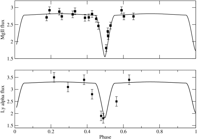
Figure 4: Integrated IUE fluxes (squares) in the ultraviolet emission lines of Mg ii h and k (top) and the Ly ${\alpha}$ (bottom) against phase with the scaled V-band model eclipse light curves for YY Gem. The IUE fluxes are in units of 10^-12 ergs cm^-2 s^-1. Note the reasonable fit of the Mg ii fluxes to the V secondary eclipse curve and the much broader eclipse in Ly${\alpha}x$.

Figure 5: H$\alpha$ line profiles of YY Gem obtained on the 5 and 6 March 1988 at the Crimean Astrophysical Observatory (see Tuominen et al. 1989). Fluxes are normalised to the continuum.

Here, $\lambda$ is the effective wavelength of the R, I or K filters being compared with V. The left side concerns empirically determined ratios of the maculation amplitudes, while the right implicitly yields corresponding spot temperatures for given wavelengths if we have some value of the mean unspotted photospheric temperature $T_{\rm p}$. We have adopted the value 3770 K given by Budding & Demircan (2007). This was determined using an absolute flux calibration, with an adopted flux of $8.82\times 10^{-12}$ W m^-2. This temperature is higher than many values for M1 stars in the literature, as noted by Torres and Ribas (2002) who preferred a yet higher value of 3820 K. The bolometric correction required to match the V flux is –1.18 mag. This is somewhat less than the value –1.25 mag that recent sources would give for this type of star (cf. di Benedetto, 1998; Bessell et al., 1998), but a higher assigned temperature would increase this discrepancy and our adopted 3770 K appears a reasonable compromise. In Table 3, column 5, we list the spot temperature differences which satisfy the aforegoing identity.

Eker’s alternative approach seems less direct, given insufficient transmission details for the three R, I and K wavebands. Here, we assume the (V–R), (V–I) and (V–K) colours of spotted regions are the same as those of a (very cool) star of the same spectral type or temperature. For the R and I bands, we first interpolated the values in Table 4 of Thé et al. (1984) to determine spectral types of the relevant spotted regions, and thence corresponding temperatures (Cox, 2000). For the K band we can find a temperature directly from the relation for log $T_{e}$ to $(V-2.2\mu)$ of Veeder (1974). Results are given in Table 3, column 6. In both methods, the mean representative temperatures of all dark spots affecting a given light curve are taken to be the same.

Empirically derived values for the difference in temperature of spots and the normal photosphere on YY Gem were found to vary from $\sim$200 K to $\sim$1200 K, with the difference from the K band larger than that from the R and I bands. The average results from Table 3 give a temperature difference of 650 $\pm$ 300 K, which appears in good agreement with the photosphere – spot temperature difference of 600 $\pm$ 450 K found by Vogt (1981) and Eker (1994) for the prototype star BY Dra (M0 V).

The disparity in the results for the mean temperatures of the spotted areas shown in Table 3 render infeasible an accurate resolution into distinct penumbral and umbral regions. While the solar case suggests a significant role for penumbra in large spots (Bray & Loughhead (1964)), the fact that derived temperature differentials for the maculation of cool active stars are generally less than that of large sunspots may well be an indication that these active regions are heterogeneous in detail, either because of complex shapes and groupings of spots, the presence of white-light faculae, penumbral components or other, perhaps temporal, irregularities.

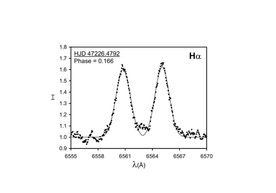
Figure 6: H$\alpha$ line profile for YY Gem with a profile model fit.

Several calculations of mean spot temperatures for RS CVn stars have been reported, giving values that differ from the normal photospheric temperature by typically $\sim$1000 K, (Vogt, 1981; Eker, 1994, Neff et al. 1995, Olah & Strassmeier, 2001, Berdyugina, 2004). This difference is lower for M type stars than for the solar type (Vogt, 1981: Rodono, 1986). At first sight, this is not surprising, as, from their relative areas, one can expect penumbrae to dominate the flux. However, Dorren (1987) argued that this is unlikely, as only spots with umbral areas $<$10% of the total spot area show penumbral flux domination. Dorren found, for practically all cases, that the increased contrast of the umbra weights the result towards the umbral component’s effect.

Berdyugina (2005) has written a comprehensive review of current techniques for the determination of starspot temperatures. In Figure 7 of that publication, starspot temperature decrements (T_P-T_S) are shown to correlate with the photospheric temperature (T_P), with both dwarfs and giants scattered about a single mean curve. The mean starspot temperature decrement we derive here for YY Gem (650$\pm$300 K) falls close to the mean line in the lower part of Berdyugina’s figure.

6 Spectroscopic Data

6.1 Ultraviolet Spectra from IUE

Observations of ultraviolet spectra from the International Ultraviolet Explorer Satellite (IUE) of YY Gem were scheduled for 5 and 6 March 1988 from 03:00 to 11:00 UT. A total of 30 spectra were obtained; 9 with the short wavelength (1000-2000 A) SWP camera and 21 with the long wavelength (2000-3000 A) LWP camera. To improve the time resolution, two exposures of 10 minutes duration were taken with the LWP camera before the image was downloaded, whereas exposures in the SWP camera were single and longer (circa 25m). The spectra obtained covered the secondary eclipse and some contiguous phases. The Starlink reduction package IUEDR was used to extract the emission line fluxes in Mg ii (2800A), Ly ${\alpha}$, C iv (1550A) and various other lines. Only the Mg ii and Ly${\alpha}$ results will be detailed here.

The most noticeable feature of the Mg ii emission during secondary eclipse is that it is fitted reasonably well by the scaled V light curve (see Figure 4 - top). This implies that the surface is approximately uniformly covered by Mg ii emitting plages. At first sight, the existence of an approximately uniform chromosphere above an evidently non-uniform photosphere might be unexpected. However, this is not the first time that such a situation has been suggested by observations. That the very active dMe stars may be totally covered (‘saturated’) with chromospheric regions was proposed by Linsky & Gary (1983) as an explanation for the high integrated Mg ii flux on BY Dra like stars. Mathioudakis & Doyle (1989) reached a similar conclusion, taking into account the integrated Mg ii and soft X-ray fluxes of dM-dMe stars.

There is some suggestion of a Mg ii flux increase towards the end of our IUE observation run. This could be associated with a lower latitude active region at longitude about 230°, but there is insufficient data to confirm this suggestion.

In Figure 4 (bottom) we show the flux in the Ly$\alpha$ line with the geocoronal emission subtracted. The extraction was made using the method of Byrne & Doyle (1988). The eclipse light curve in Ly$\alpha$ appears broader than the V-band curve. We should note, however, that there are only a few data points at relevant phases, and the out-of-eclipse scatter shows deviations that are comparable. There are two feasible explanations; one of them intrinsic to the star and the other not. The first alternative would be that the broad eclipse arises from a larger volume of Ly${\alpha}$ emitting material than the photosphere of the secondary star, roughly centred on that star. In effect, this extended region would be optically thick in Ly${\alpha}$. Another explanation for the broad decline at secondary minimum in Ly${\alpha}$ could be variable absorption by interstellar H as the emission lines of the orbiting stars are Doppler shifted across the rest wavelength of the interstellar absorption line. This is unlikely to be significant, however, due to the small range in radial velocity $\sim$15% at eclipses when the stellar motion is perpendicular to the line of sight. We conclude, therefore, that the Ly${\alpha}$ light curve reflects the scale of the stellar outer atmosphere, i.e. optically thick conditions at Ly${\alpha}$ out to heights of the order of twice the photospheric radii (cf. Aschwanden, 2004). This is quite different to the situation for the H${\alpha}$ data that we examine next. For H${\alpha}$, the predominant formation layer appears to be located at a relatively low height above the photosphere.

6.2 Optical Spectra

Optical spectra covering the H${\alpha}$ region were obtained with the coude Spectrograph on the 2.6^m Shajn telescope at the Crimean Astrophysical Observatory on 5 and 6 March 1988 with ten spectra obtained on the first night and nine on the second (see Tuominen et al. 1989). The H${\alpha}$ emission at various phases close to and out of eclipse are shown in Figures 5 and 6. These profiles were modelled using the program PROF (Olah et al, 1992) where the assumption is made that the emission flux at a particular wavelength is proportional to the number of atoms in the line of sight emitting at that wavelength. The program numerically integrates Doppler and Gaussian broadening contributions for each of the ten slices across the projected stellar surface.

The results are listed in Table 4. In this table the parameters $I_{0}$, $\lambda_{0}$, $r$ and $s$ give the peak intensity, mean wavelength, rotational and Gaussian broadening coefficients respectively for those emission line profiles which could be separated into two components. We note a high degree of self-consistency in the rotation parameter, implying mean equatorial rotational velocities of 38.6 and 38.5 km s^-1 ($\pm$0.1 km s^-1) for the primary and secondary respectively. If we use the orbital velocity sum of Torres & Ribas (2002) and assume co-rotation of the components, we find a pair of essentially equal-sized stars, but with radii some 4% bigger than those derived from the broadband light curves. In other words, there is evidence for a small but significant scale of chromospheric enhancement from the H${\alpha}$ profiles. The scatter of the Gaussian component from profile to profile is significantly bigger than that of the rotation parameter, indicating a detectable variability of local surface turbulence that could be associated with local inhomogeneities of velocity. This picture is consistent with that of the Sun where various H$\alpha$ emission features such as spicules and prominences etc regularly appear above the surface, particularly when active regions are close to the limb. A dMe star, such as YY Gem, with its much higher level of activity would be expected to show extensive off-disk structures

Table 4: Parametrisation of PROF fittings to the H$\alpha$ emission lines shown in Fig 5.

HJD	Comp.	$I_{0}$	$\lambda_{0}$(Å)	r(Å)	s(Å)
47226.3736	2	1.401	6562.848	0.840	0.854
$\phi$ = 0.036	•	$\pm 0.015$	$\pm 0.012$	$\pm 0.010$	$\pm 0.013$
	1	0.768	6561.400	0.838	0.710
47226.4444	•	$\pm 0.013$	$\pm 0.017$	$\pm 0.017$	$\pm 0.021$
$\phi$ = 0.123	2	0.629	6564.411	0.838	0.705
		$\pm 0.013$	$\pm 0.023$	$\pm 0.025$	$\pm 0.027$
	1	0.935	6561.054	0.833	0.827
47226.4681		$\pm 0.015$	$\pm 0.017$	$\pm 0.015$	$\pm 0.020$
$\phi$ = 0.152	2	0.749	6564.745	0.843	0.762
		$\pm 0.013$	$\pm 0.020$	$\pm 0.019$	$\pm 0.023$
	1	0.884	6560.765	0.841	0.789
47226.4792		$\pm 0.014$	$\pm 0.017$	$\pm 0.015$	$\pm 0.020$
$\phi$ = 0.166	2	0.909	6565.089	0.841	0.777
		$\pm 0.014$	$\pm 0.016$	$\pm 0.015$	$\pm 0.019$
	1	0.816	6560.560	0.844	0.768
47226.5125		$\pm 0.013$	$\pm 0.018$	$\pm 0.016$	$\pm 0.020$
$\phi$ = 0.206	2	0.837	6565.290	0.841	0.751
		$\pm 0.013$	$\pm 0.017$	$\pm 0.016$	$\pm 0.020$
	1	0.813	6560.562	0.847	0.763
47227.3132	•	$\pm 0.013$	$\pm 0.018$	$\pm 0.017$	$\pm 0.020$
$\phi$ = 0.190	2	0.682	6565.043	0.845	0.742
		$\pm 0.013$	$\pm 0.021$	$\pm 0.019$	$\pm 0.024$
	1	0.927	6560.335	0.844	0.791
47227.3361		$\pm 0.014$	$\pm 0.016$	$\pm 0.015$	$\pm 0.019$
$\phi$ = 0.218	2	0.748	6565.265	0.830	0.793
		$\pm 0.014$	$\pm 0.020$	$\pm 0.018$	$\pm 0.024$
	1	0.822	6560.223	0.840	0.684
47227.3597		$\pm 0.013$	$\pm 0.016$	$\pm 0.015$	$\pm 0.019$
$\phi$ = 0.247	2	0.677	6565.435	0.835	0.704
		$\pm 0.014$	$\pm 0.019$	$\pm 0.019$	$\pm 0.024$
	1	0.815	6560.218	0.843	0.719
47227.3875		$\pm 0.013$	$\pm 0.017$	$\pm 0.016$	$\pm 0.020$
$\phi$ = 0.281	2	0.705	6565.411	0.839	0.754
		$\pm 0.013$	$\pm 0.020$	$\pm 0.019$	$\pm 0.024$
	1	0.911	6560.319	0.843	0.720
47227.4111		$\pm 0.013$	$\pm 0.015$	$\pm 0.141$	$\pm 0.017$
$\phi$ = 0.310	2	0.720	6565.366	0.838	0.725
		$\pm 0.013$	$\pm 0.019$	$\pm 0.019$	$\pm 0.023$
	1	1.159	6560.520	0.845	0.843
47227.4410		$\pm 0.014$	$\pm 0.014$	$\pm 0.012$	$\pm 0.015$
$\phi$ = 0.347	2	0.770	6565.224	0.845	0.748
		$\pm 0.013$	$\pm 0.018$	$\pm 0.017$	$\pm 0.021$
	1	1.042	6560.738	0.838	0.824
47227.4646		$\pm 0.015$	$\pm 0.015$	$\pm 0.013$	$\pm 0.017$
$\phi$ = 0.376	2	0.661	6564.982	0.847	0.730
		$\pm 0.013$	$\pm 0.021$	$\pm 0.020$	$\pm 0.025$

From Figure 5, we note that at quadrature (phase $\sim$ 0.25), when the primary component is approaching the observer (blue-shifted spectrum), the H${\alpha}$ line from the primary is approximately 20% brighter than that from the secondary. Likewise, in Table 4, we see that the ratio of the central intensities of the two components (primary/secondary) is around 1.2 for the three spectra near phase 0.25 (0.218, 0.247, 0.281) rising to 1.5 for the two spectra with phase 0.347 and 0.376. At this phase the largest spot listed in Table 2, with longitude 94.8^∘ and latitude $\neg$16^∘ would be on the facing hemisphere of the primary component. A reasonable explanation for this would be that a bright H${\alpha}$ emission region on the primary was topologically associated with a dark spot on the same component.

7 X-ray and Radio observations

7.1 X-ray data from GINGA

YY Gem was observed with the Ginga (ASTRO-C) satellite, using its Large Area proportional Counter (LAC) from 09:00 UT on March 4 until 11:00 UT on March 6. Turner et al. (1989) give details of Ginga, and a full description of the LAC instrument including its design, construction, calibration, operation, energy range, resolution, and sensitivity.

Primarily because of Ginga’s low-Earth orbit, good quality reduced data on YY Gem was obtained only intermittently during the overall period listed above, in between Earth occultations, passages through the South Atlantic Anomaly, and times when background subtraction was otherwise relatively uncertain. Reduction of the data was performed at Rutherford Appleton Laboratory using the University of Leicester’s Ginga software. The time periods with best coverage and data quality were approximately 10:00 to 15:00 UT on March 4 (see Figure 7 below), 11:00 to 19:00 UT on March 5, and 06:00 to 11:00 UT on March 6. Sparse data were also obtained at other intervening times, e.g. immediately after the period shown in Figure 7, namely from 16:00 UT on March 4 to 05:00 UT on March 5. Further details of the observations are given with the supplementary electronic tables. The quiescent X-ray emission during these observations indicates two components with temperatures 3-4MK (soft) and 40-50MK (hard).

A flare which occurred shortly after the beginning of observations on 4 March had a two-component flare emission of 3 MK and 30-35 MK. In both the quiescent and the flare situations the low-temperature (soft) component makes up about 10% of the total flux over the 2-10 KeV range. Both flare and quiescent spectra showed only weak Fe xxv emission at 6.7 keV. Fits to the X-ray spectra were improved if the Fe-abundance was reduced to 0.5 solar.

In Figure 7, we see that the flare begins to rise above quiescent level around 10:12 to 10:15 UT (HJD $\sim$ 2447224.92) and reaches a maximum at around 10:45 UT (HJD $\sim$ 2247224.94). The estimated integrated X-ray luminosity is about 3-4 10³³ ergs (2-10 KeV). The flare light curve can be very well represented by the magnetic reconnection model of Kopp & Poletto (1984) and Poletto, Pallavicini & Kopp (1988). For example, using a time constant of around 2.5 hours (i.e. the time constant of the underlying reconnection process) and a start time of 10:15 UT, the predicted light curve fits the rise and peak very well, and is a reasonable fit to the late decay phase. The long duration of the X-ray event and the agreement with this model, tends to favour interpretation as a solar-like, two-ribbon, flare event. In solar terms this equates to an X30-X40 class flare, equivalent to the largest solar flare ever observed. As with the increased H$\alpha$ emission mentioned in the previous section, we note that the flare detected in X-rays on 4 March, occurred at binary phase $\sim$0.27, i.e. close to quadrature and the phase of maximum visibility of the large spot identified in Section 4 and Table 2.

The X-ray data suggest a fairly continuous, relatively active state of the components of YY Gem, that can probably be associated with micro-flaring, since only a single large flare was observed during the campaign. The background level in X-rays has a significant hard component that is even harder than during the flares. This background may well be associated with the same electrons that give rise to the more or less continuous microwave emission.

The flare seen in X-rays by Ginga was also observed optically with the 0.6^m reflector on Mauna Kea. For most of the duration of the flare, observations with this telescope were sporadic, intended for spot modulation rather than continuous monitoring for flare activity. The U and B observations over this period are shown as filled black squares in the lower two panels of Figure 7. With only three or four U/B observations during the gradual phase of the flare, the precise shape of the light curve at this time is uncertain. Nevertheless, we believe that a reasonable estimate of the integrated optical flux during the gradual phase of the flare can be derived from the data. We estimate the total integrated flare energy for the gradual phase of the flare to be $8\times 10^{33}$ ergs and $27\times 10^{33}$ ergs in the U and B bands, respectively.

For a period of around 18 minutes the mode of observation was changed to continuous U-band monitoring with a time resolution of approximately 6 seconds. This data which has been corrected for extinction and converted to magnitudes is shown in the middle panel of Figure 7 with filled circles. By chance, the observations captured the impulsive phase of the optical flare which sits on top of the gradual flare described above. The integrated U-band energy of the impulsive phase is $\sim 6\times 10^{32}$ ergs, i.e. about an order of magnitude less than the U-band energy of the gradual phase. Assuming the ratio of the U-band to B-band fluxes to be the same for the impulsive stage of the flare as for the gradual phase, we derive a total optical energy in the near ultraviolet/blue region of the spectrum for both stages of the flare of $37\times 10^{33}$ ergs and a ratio of X-ray to optical flux $\sim$ 0.09. This is close to the values for flares on UV Ceti ($\sim$ 0.2), YZ CMi ($\sim$ 0.1) and AD Leo ($\sim$ 0.1-0.2), listed by Katsova (1981). In her summary, Katsova (1981) notes that values L_X/L_opt $\sim$ 0.1 - 0.2 are consistent with expectations for a flare eruption from a closed magnetic field configuration. Table 5 summarises the flare energetics from this campaign.

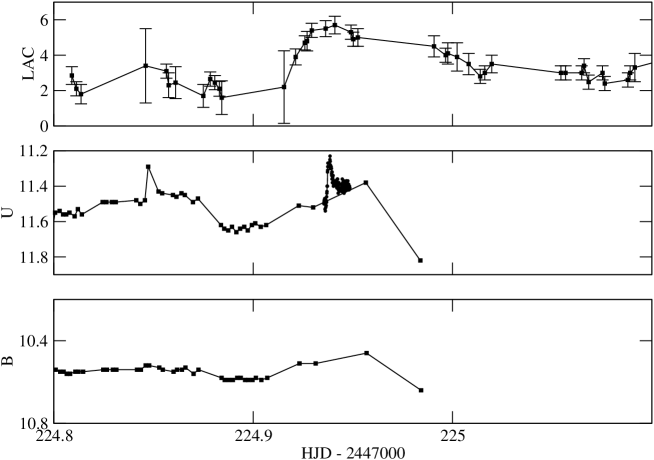
Figure 7: The flare on YY Gem observed optically and in X-rays by the Ginga Satellite on 4 March 1988. Top - X-ray count rate in the Large Area Proportional Counter (LAC); Middle and Bottom - U and B band photometry from 60cm telescope on Mauna Kea

7.2 Microwave observations from the VLA

YY Gem was observed in the microwave region with the VLA on two successive days, March 4/5 and 6, 1988. The VLA was operated in two sub-arrays: one observing continuously at C band (6cm; 4.8 Ghz), and the other alternating between X band (3.6 cm; 8.4 GHz) and L band (20cm; 1.46 GHz). It was detected in both the shorter wavelengths but not at 20cm. Figure 8 shows the 6 cm flux curve of the system from the observations made on 4/5 March. Both the primary (phase = 1.0) and secondary (phase = 1.5) eclipses appear to be visible in the flux curves with a slight shift of about 0.03 in the phase of minima compared to the V-band light curve. Both radio eclipses appear to be significantly narrower (by a factor $\sim$2) than the optical eclipses. The 6 cm flux at primary minimum falls close to zero which indicates that most if not all the 6 cm emission lies on the side of the primary facing the secondary or in the space between the two components. This is similar to that found on the RSCVn binary CF Tuc by Gunn et al (1997). At secondary eclipse, (phase $\sim$1.5) the 6 cm flux falls to about 50% of the normal non-eclipsed level. The secondary eclipse does not appear in observations made on 6 March. These apparent eclipses cannot be considered definitive, however, as comparable variations are seen elsewhere in the microwave data at times that definitely cannot be attributed to eclipses. If the feature at phase 0.98 is an eclipse it would suggest a radio emitting region somewhat displaced towards the advancing hemisphere.

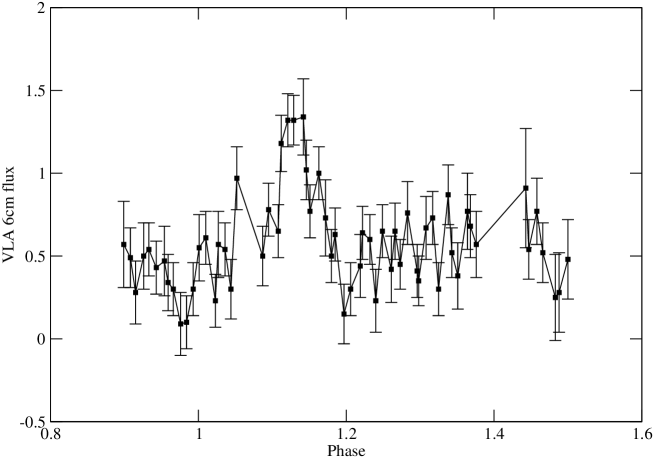
Figure 8: The 6-cm microwave flux (in mJy) from the VLA for YY Gem on 4/5 March with one sigma error bars

On the 5th March at approximately 03:00 UT a large flare was seen in 6 cm emission that lasted for one and a half to two hours. This flare was also observed in the optical at McDonald Observatory. In Figure 9 we show the 6-cm flux curve together with the U and B band photometry for the impulsive part of the flare followed by its prolonged decline. We note that this flare occurs at binary phase $\sim$0.15, i.e. not far from quadrature.

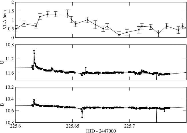
Figure 9: The flare observed in 6-cm emission on 5 March by the VLA and simultaneously in the optical at the McDonald Observatory. Top - 6-cm microwave flux in mJy; Middle and Bottom - U and B band light curves

From the optical light curves of the flare we derive a peak flux of approximately 7.4 x 10³⁰ ergs s^-1 and 5.9 x 10³⁰ ergs s^-1 in U and B respectively. Total integrated flare energies were found to be almost identical in U and B at 2.1 x 10³³ ergs giving a total optical energy of the order of 5 x 10³³ ergs. One third of this energy comes from the long tail of the flare which lasted approximately one hour in the optical and 1.7 hours in the radio.

The peak flux at 6cm during the flare reaches 0.9 mJy, equivalent to a total emitted flux at flare maximum of 2.4 x 10¹⁴ ergs s^-1 Hz^-1. The measured time-averaged radio flux, on the other hand, is 1.6 x 10¹⁴ ergs s^-1 Hz^-1. Using Figure 6 from Benz & Gudel (1994), which relates the time-averaged X-ray and radio fluxes for active stars, we can estimate the soft X-ray flux from the measured VLA flux for the above flare on YY Gem. We obtain a value for the time-averaged soft X-ray flux of $3\times 10^{29}$ ergs s^-1. Assuming the flare lasted as long in X-rays as at 6cm radio wavelengths (namely, $\sim$ 1.7 hours), we derive an integrated flare energy in soft X-rays of $1.8\times 10^{33}$ ergs. With an observed optical energy for the same flare of $\sim 5\times 10^{33}$ ergs from above, we obtain a value of L_X/L${}_{opt}\sim 0.36$, in reasonable agreement with that observed directly by Ginga described in Section 7.1 and on flares on other stars given by Katsova (1981).

Regrettably, because the periods with successful Ginga data were so sporadic, there is limited overlap between the VLA and Ginga observation windows. Nevertheless, it appears that Ginga did just catch the tail end of the VLA/optical flare on 4 March. However, the single Ginga data point obtained at this time is quite inadequate to give quantitative information on the strength of the coincident X-ray flare.

Table 5: Integrated optical and X-ray energies of flares on YY Gem in units of 10³³ ergs

UT (max)	HJD (max)	U-band	B-band	Lopt	X-ray (2-10KeV)	LX/Lopt
March 4 10:45	2247224.94	8.6	29	37	3-4	0.09
March 5 03:00	2247225.62	2.1	2.1	5	$\sim$ 1.8	0.36

8 Conclusions

The March 1988 coordinated multiwavelength campaign on YY Geminorum resulted in less extensive ground-based coverage than originally planned. This was principally due to the exceptionally bad weather which prevailed in the Canary Islands at that time. Nevertheless, useful data were obtained from ground-based facilities in the western hemisphere, notably the VLA and Mauna Kea in Hawaii, as well as space-based facilities on board the IUE and Ginga satellites.

With the aid of computer modelling of the V-band eclipse light curve, we obtain almost identical luminosities and radii for the two components of YY Gem and, when combined with previously published radial velocity curves, masses of $0.6M_{o}$ and radii of $0.601R_{o}$ are derived. Fits to the out-of-eclipse light curves with spot models give two cool spots roughly $165^{o}$ apart in longitude and at latitudes of $-16^{o}$ and $45^{o}$ and one bright spot at $21^{o}$ latitude. Due to the high orbital inclination, there is significant ambiguity in the latitudes derived and it is not possible to determine on which component the maculation occurs. Combining these models with the additional broad-band colours B, R, I and K, allows estimates to be made of the temperature differential between the cool spots and the normal photosphere. We estimate a value of $650^{o}\pm 300$, closely similar to previous results by Vogt (1981) on BY Draconis. Analysis of the line profiles of H$\alpha$ in contemporaneous spectra of YY Gem indicates that the radii of the H$\alpha$ emission volumes are about 4% larger than the optical radii.

We have observed the secondary eclipse of YY Gem in the ultraviolet emission lines of Mg II and Ly$\alpha$ with the IUE satellite. When scaled, the Mg II eclipse light curve is fitted well by the V-band light curve, indicating the presence of a chromosphere on YY Gem with uniformly emitting Mg II from contiguous plage regions. The existence of a widespread network of emission in the chromospheric lines of CaII and MgII on the Sun has been known for many years (see Phillips, 1992). A similar picture emerges from studies of many spotted stars where high levels of MgII line flux have been observed along with a relatively small degree of rotational modulation (see Butler et al. 1987; Butler, 1996). The Ly$\alpha$ light curve of YY Gem, on the other hand, has a much broader secondary eclipse suggesting an extended outer atmosphere with a height of the order of twice the radius.

YY Gem was detectable with the VLA at both 3.6 and 6 cm wavelengths but not at 20cm. Both the primary and secondary eclipses appear in the 6cm light curve on 5 March but on the following day the secondary eclipse is no longer evident. A poor signal-to-noise ratio prevents us from drawing any definitive conclusions about either eclipse at radio wavelengths, however there are indications that both the primary and secondary eclipses are narrower and slightly offset in phase in 6 cm emission compared to the optical V-band which would be indicative of relatively compact radio emitting regions. The almost total primary eclipse compared to a drop to only half the uneclipsed flux at the secondary eclipse would suggest that the emitting region on the primary is more compact than that on the secondary.

Four flares which were detected optically on YY Gem during this campaign and have been reported earlier showed evidence of periodicity (see Doyle et al. (1990). Two possible mechanisms which could have given rise to the periodicity are: (1) oscillations in magnetic filaments associated with the flares, or (2) fast magneto-acoustic waves between the binary components as described by Gao et al. (2008).

In this paper we show optical observations of two further flares on YY Gem, one of which was also seen in soft X-rays by the Ginga satellite and the other in 6-cm radiation by the VLA. Estimates of the integrated optical energy, based on the photometry are possible for both flares. For the flare seen by Ginga, we can also derive the integrated soft X-ray flux, leading to an estimate for the ratio of the integrated X-ray to optical energy, L_X/L_opt $\sim$ 0.1, closely similar to the ratio observed in flares on other dMe stars. The well established correspondence between the soft X-ray and radio fluxes by Benz & Gudel (1994) allows us to make an indirect estimate of the soft X-ray energy of the flare seen by the VLA and thereby estimate L_X/L_opt for this additional flare.

The ratio L_X/L_opt for both YY Gem flares lies close to the value predicted by Katsova’s gas-dynamic model of a stellar flare in a constrained magnetic loop. If this ratio was $\sim$ 1000, as found for some solar flares, it would indicate, according to Katsova, an origin in an open magnetic structure where evaporation precluded excessive heating of the affected plasma.

Lastly, we note the coincidence in binary phase of several indicators of magnetic activity on YY Gem. The flares observed in X-rays and the radio region occurred at phases 0.27 and 0.15 respectively; i.e. within the phase interval during which the largest spot at longitude 94.8^∘ would be visible. Spectroscopic data obtained as part of this campaign also provides evidence of an H$\alpha$ emission region on the primary component with increasing visibility from phase 0.25 to 0.35. A reasonable interpretation of these observations would be that all are manifestations of magnetic activity from a single large active region on the primary component of YY Gem. This is not an unexpected conclusion as similar associations between flares, H$\alpha$ emission regions and spots are common on the Sun and have been seen previously on other stellar systems (see Rodono et al. 1987, Olah et al. 1992, Butler, 1996).

9 Appendix A - The electronic data files

The observational data accumulated during this project and presented in the figures shown in this paper are available via the Internet from the Armagh Observatory World-Wide Web Site using the link: http://www.arm.ac.uk/preprints/2014/654 with subdirectories /photometry, /spectroscopy, /IUE, /VLA and /Ginga containing the optical photometry, the spectroscopic, ultraviolet, radio and X-ray data respectively. In each subdirectory a file ”notes-etc” contains a description of the data available and the format of each file. A subdirectory /figures contains the encapsulated postscript files for the figures displayed here.

References

- [\citeauthoryearAdams1917] Adams, W.S. and Joy, A.H., 1917, Astrophys. J. 46, 313
- [\citeauthoryearAschwanden2004] Ashwander, M.J., 2004, Physics of the Solar Corona: An introduction, Praxis, Chichester, UK
- [\citeauthoryearBaliunas2006] Baliunas, S.L. 2006, IAU Joint Discussion No 8: Solar and Stellar Activity Cycles, August 2006, Prague, Highlights of Astronomy 14, K.G. Strassmeier and A. Kosovichev (eds), 65
- [\citeauthoryearBarnes et al.1976] Barnes, T.G. and Evans, D.S., 1976, Mon. Not. R. Astron. Soc. 174, 489
- [\citeauthoryearBenz1994] Benz, A.O., Gudel, M, 1994, Astron. Astrophys. 285, 621-630, 1994
- [\citeauthoryearBerdyugina2004] Berdyugina, S.V. 2004, Sol. Phys. 224, 123
- [\citeauthoryearBerdyugina2005] Berdyugina, S.V. 2005, Living Rev. Sol. Phys. 2, 8.
- [\citeauthoryearBessell1979] Bessell, M.S., 1979, P. Astron. Soc. Pac. 91, 589.
- [\citeauthoryearBessell et al1998] Bessell, M.S., Castell, F. and Plez, B., 1998, Astron. & Astrophys. 333, 231
- [\citeauthoryearBevington1969] Bevington, P.R., 1969, Data Reduction and Error Analysis for the Physical Sciences, McGraw-Hill, New York
- [\citeauthoryearBopp1973] Bopp, B.W. and Evans, D.S., 1973, Mon. Not. R. Astron. Soc. 164, 343
- [\citeauthoryearBray1964] Bray, R.J., and Loughhead, R.E., 1964, Sunspots, Chapman and Hall, London
- [\citeauthoryearBudding et al..1974] Budding, E. and Kitamura, M., 1974, IBVS 900, 1
- [\citeauthoryearBudding et al.1987] Budding, E. and Zeilik, M., 1987, Astrophys. J. 319, 827
- [\citeauthoryearBudding et al.1996] Budding, E., Butler, C.J., Doyle, J.G., Etzel, P.B., Olah, K., Zeilik, M. and Brown, D., 1996, Astrophys. Space Sci. 236, 215
- [\citeauthoryearBudding et al2005] Budding, E., Rhodes, M. and Sullivan, D.J., 2005, Transit of Venus: New views of the Solar System and Galaxy, Proc. IAU Colloquium 196, 7-11 June 2004, Preston, UK, D.W. Kurtz (ed), Cambridge Univ. Press, 386
- [\citeauthoryearBudding Demircan2007] Budding, E. and Demircan, O., 2007, Introduction to Astronomical Photometry, Cambridge
- [\citeauthoryearButler1987] Butler, C.J., Doyle, J.G., Andrews, A.D., Byrne, P.B., Linsky, J.L., Bornmann, P.L., Rodono, M., Pazzani, V. and Simon, Theodore, 1987, Astron. Astrophys. 174, 139
- [\citeauthoryearButler1988] Butler, C.J., 1988, IBVS 3128
- [\citeauthoryearButler1994] Butler, C.J., Doyle, J.G., Budding, E. and Foing, B. 1994, Proc. MUSICOS Workshop, Beijing, July 1994, ESA/ESTEC, 207
- [\citeauthoryearButler1995] Butler, C.J., Doyle, J.G. and Budding, E. 1995, proc. 9th Cambridge Cool Star Workshop, Florence, October 1995, R. Pallavicini and A. Dupree (eds), ASP Conf. Ser. 109, 589
- [\citeauthoryearButler1996] Butler, C.J., 1996, proc. IAU Symp. 176 Stellar Surface Structure, Vienna, October 1995. K. Strassmeier and J. Linsky (eds), Kluwer, 423
- [\citeauthoryearByrne et al1988] Byrne, P.B. and Doyle, J.G., 1988, A decade of UV astronomy with the IUE satellite, 12-15 April 1988, ESA SP-281, 319
- [\citeauthoryearChabrier1995] Chabrier, G. and Baraffe, I., 1995, Astrophys. J. 451, L29
- [\citeauthoryearCousins1980] Cousins, A.W.J., 1980 , S.A.A.O. Circ. No 5, 234
- [\citeauthoryearCousins1984] Cousins, A.W.J., 1984, S.A.A.O. Circ. No 8, 69
- [\citeauthoryearCox2000] Cox, A. N. (ed), 2000, Astrophysical Quantities, 4th Edition, Springer, New York
- [\citeauthoryeardi Benedetto] di Benedetto, G.P. 1998, Astron. & Astrophys. 339, 858
- [\citeauthoryearDonati2003] Donati, J.-F., et al. (10 co-authors), 2003, Mon. Not. R. Astron. Soc. 345, 1145
- [\citeauthoryearDorren1987] Dorren, J.D., 1987, Astrophys. J. 320, 756
- [\citeauthoryearDoyleButler1985] Doyle, J.G. and Butler, C.J., 1985, Nature 313, 378
- [\citeauthoryearDoyle et al.1990] Doyle, J.G. and Mathioudakis, M., 1990, Astron. & Astrophys. 227,130
- [\citeauthoryearDoyle et al.1990] Doyle, J.G., Van den Oord, G.H.J., Butler, C.J. and Kiang, T., 1990, Astron. & Astrophys. 272, 83
- [\citeauthoryearEker1994] Eker, Z., 1994, Astrophys. J. 420, 373
- [\citeauthoryearGao2008] Gao, D.H., Chen,P.F., Ding, M.D. & and Li, X.D., 2008, Mon. Not. R. Astr. Soc. 384, 1355
- [\citeauthoryearGary1986] Gary, D.E., 1986, Cool Stars, Stellar Systems and the Sun, Lecture Notes in Physics, 254, M. Zeilik and D. Gibson (eds), Springer-Verlag, New York, 235.
- [\citeauthoryearGunn1997] Gunn, A.E., Migeres, V., Doyle, J.G., Spencer, R.E. & Mathioudakis, M. 1997, Mon. Not. R. Astr. Soc. 237, 199
- [\citeauthoryearHaisch et al1990] Haisch, B.M., Schmitt, J.H.M., Rodono, M. and Gibson, D.M., 1990, Astron. & Astrophys. 230, 419.
- [\citeauthoryearJackson et al1989] Jackson, P.D., Kundu, M.R. and White, S.M., 1989, Astron. & Astrophys. 210, 284
- [\citeauthoryearJoy1926] Joy, A.H. and Sandford, R.F., 1926, Astrophys. J. 64, 250
- [\citeauthoryearKopp et al1984] Kopp, R. A. and Poletto, G. 1984, Solar Phys. 93, 351
- [\citeauthoryearKatsova1981] Katsova, M.M., 1981, Sov. Astron. 25 (2), 197
- [\citeauthoryearKrisciunas et al.1987] Krisciunas, K., Sinton, W., Tholen, K., Tokunaga, A., Golisch, W., Griep, D., Kaminski, C., Impey, C., Christian, C., 1987, PASP, 99, 887K
- [\citeauthoryearKron1947] Kron, G.E., 1947, Pub. Astron. Soc. Pac. 59, 261
- [\citeauthoryearKron1950] Kron, G.E., 1950, Astron. Soc. Pac. Leaflets 6, No 257, 52
- [\citeauthoryearKron1952] Kron, G.E., 1952, Astrophys. J. 115, 301
- [\citeauthoryearLacy1976] Lacy, C.H., Moffett, T.J. and Evans, D.S., 1976, Astrophys. J. Suppl. Ser. 30, 85
- [\citeauthoryearLinsky1983] Linsky, J.L. and Gary, D.E., 1983, Astrophys. J. 274, 776
- [\citeauthoryearMathioudakis1989] Mathioudakis, M. and Doyle, J.G., 1989, Astron. & Astrophys. 224, 179
- [\citeauthoryearMoffat et al1979] Moffat, T.J. and Barnes, T.G., 1979, Astron. J. 84, 627
- [\citeauthoryearNeff et al1995] Neff, J.E., O’Neal, D., Saar, S.H., 1995, Astrophys. J. 452, 879
- [\citeauthoryearOlah-strass2001] Olah, K. and Strassmeier, K.G. 2001, 11th Cambridge Workshop on Cool Stars, Stellar Systems and the Sun, ASP Conference Proceedings, Vol. 223. Ramon J. Garcia Lopez, Rafael Rebolo, and Maria Rosa Zapaterio Osorio (eds). Astronomical Society of the Pacific, ISBN: 1-58381-055-2, p.1030
- [\citeauthoryearOlah et al1992] Olah, K., Butler, C.J., Houdebine, E.R., Gimenez, A. and Zeilik, M. 1992, Mon. Not. R. Astron. Soc. 259, 302
- [\citeauthoryearPearson1954] Pearson, E.S. and Hartley, H.O. 1954, Biometricia Tables for Statisticians 1, Cambridge
- [\citeauthoryearPetit2004] Petit, P. et al (10 co-authors), 2004, Mon. Not. R. Astron. Soc. 348, 1175
- [\citeauthoryearPhillips1992] Phillips, K.J.H., 1992, Guide to the Sun, Cambridge, 107
- [\citeauthoryearPoletto1988] Poletto, G., Pallavacini, R. and Kopp, R.A., 1988, Astron. & Astrophys. 201, 93
- [\citeauthoryearPopper1998] Popper, D. 1998, Pub. Astron. Soc. Pac. 110, 919
- [\citeauthoryearQian et al2002] Qian, S., Liu, D., Tan, W. and Soonthornthum, B. 2002, Astron. J. 124, 1060
- [\citeauthoryearRadick1998] Radick, R.R., Lockwood, G.W., Skiff, B.A. and Baliunas, S.L. 1998, Astrophys. J. Suppl. 118, 239
- [\citeauthoryearRodono1987] Rodono, M., Byrne, P.B., Neff, J.E., Linsky, J.L., Simon, T., Butler, C.J., Catalano, S., Cutispoto, G., Doyle, J.G., Andrews, A.D. and Gibson, D.M. 1987, Astron. and Astrophys. 176, 267
- [\citeauthoryearSaar et al2003] Saar, S.H. and Bookbinder, J.A., 2003, The Future of Cool Star Asrophysics: 12th Cambridge Workshop on Cool Stars, Stellar Systems and the Sun, A. Brown, G.M. Harper and T.R. Ayres (eds), Univ. Colorado, 1020.
- [\citeauthoryearSemeniuk2000] Semeniuk, I., 2000, Acta Ast. 50, 381
- [\citeauthoryearStelzer et al2002] Stelzer, B., Burwitz, V., Audard, M., Guedd, M., Ness, J., Grosso, N., Neuhaeuser, R., Schmitt, J.H.M.M., Predehl, P. and Aschedbach, B., 2002, Astron. & Astrophys. 392, 585
- [\citeauthoryearStrassmeir et al1996] Strassmeier, K.G. and Linsky, J.L. (eds) 1996, Stellar Surface Structure, proc. IAU Symp. 176, Vienna, October 1995, Kluwer
- [\citeauthoryearStrassmeir1992] Strassmeir, K. 1992, Astronomical Society of the Pacific Conference Series 34, 39
- [\citeauthoryearTorres2002] Torres, G. and Ribes, I., 2002, Astrophys. J. 567, 1140
- [\citeauthoryearTurner1989] Turner, M.J.L. and 16 other authors, 1989, Pub. Astron. Soc. Japan 41, 345
- [\citeauthoryearTsikoudi2000] Tsikoudi, V. and Kellett, B.J., 2000, Mon. Not. R. Astron. Soc. 319, 1147
- [\citeauthoryearTuominen et al1989] Tuominen, I, Huovelin, J., Efimov, Yu. S., Shakhovskoy, N.M. and Scherbakov, A.G., 1989, Sol. Phys. 121, 419
- [\citeauthoryearBaird1984] Thé, P.S., Steenman, H.C. and Alcaino, G., 1984, Astron. & Astrophys. 132, 385
- [\citeauthoryearvan Hamme1993] Van Hamme, W. 1993, Astron. J. 106, 2096
- [\citeauthoryearVrsnak et al.2007] Vrsnak, B., Veronig, A.M., Thalman, J.K. and Zic, T., 2007, Astron. & Astrophys. 471, 295
- [\citeauthoryearVeeder1974] Veeder, G.J., 1974, Astron. J. 79,1056
- [\citeauthoryearVogt1981] Vogt, S.S., 1981, Astrophys. J. 250, 327
- [\citeauthoryearZeilik et al.1988] Zeilik, M., de Blasi, C., Rhodes, M. and Budding, E., 1988, Astrophys. J. 332, 293