Higher order dispersive effects in regularized Boussinesq equation

Abstract

In this paper, we consider the higher order Boussinesq (HBq) equation which models the bi-directional propagation of longitudinal waves in various continuous media. The equation contains the higher order effects of frequency dispersion. The present study is devoted to the numerical investigation of the HBq equation. For this aim a numerical scheme combining the Fourier pseudo-spectral method in space and a Runge Kutta method in time is constructed. The convergence of semi-discrete scheme is proved in an appropriate Sobolev space. To investigate the higher order dispersive effects and nonlinear effects on the solutions of HBq equation, propagation of single solitary wave, head-on collision of solitary waves and blow-up solutions are considered.

1 Introduction

The first attempt to describe the solitary waves of Scott Russell’s experiment in 1834, theoretically, was made by Boussinesq [1, 2, 3]. To model the motion of the long waves in shallow water he proposed the Boussinesq equation

$$u_{tt}=u_{xx}-\frac{3\beta}{2}(u^{2})_{xx}+\frac{\beta}{3}u_{xxxx}.$$ (1.1)

We refer the reader to [4, 5] for a more detailed information on the origins of Boussinesq equation. As the equation (1.1) turned out to be incorrect in the sense of Hadamard, several re-derivations are made. The most common well-posed re-derivation is proposed for ion-sound waves and for quasi-continuum approximation of dense lattices [6, 7] and is called the ”improved” Boussinesq equation (IBq)

$$u_{tt}=u_{xx}+u_{xxtt}+(f(u))_{xx}.$$ (1.2)

Unlike the Boussinesq equation (1.1), the IBq equation is not fully integrable. The Boussinesq equation and its re-derivations include the lowest order effects of frequency dispersion. To include the higher order effects of dispersion, Rosenau [8] proposed the higher order Boussinesq (HBq) equation

$$u_{tt}=u_{xx}+\eta_{1}u_{xxtt}-\eta_{2}u_{xxxxtt}+(f(u))_{xx}$$ (1.3)

where $\eta_{1}$ and $\eta_{2}$ are real positive constants. In Rosenau’s own words ”lowest order dispersion shows some anomalous which can be resolved only if higher order discrete effects are included.” A more recent derivation of the HBq equation is given by Duruk et al. in [9] to model the bi-directional propagation of longitudinal waves in an infinite, nonlocally elastic medium. Eliminating the effects of the higher order dispersion, the HBq equation reduces to the IBq equation.

The local and global well-posedness of the Cauchy problem for the HBq equation together with the initial conditions

$$u(x,0)=\phi(x),\hskip 20.0ptu_{t}(x,0)=\psi(x)$$ (1.4)

was proved in [9] in the Sobolev space $H^{s}$ with any $s>1/2$. The same authors also studied the qualitative properties of a general class of nonlocal equations which includes the HBq equation as a special case in [10].

The present study addresses the answers of the following very natural questions: How the higher-order dispersive term and the various power type nonlinear terms, i.e. $f(u)=\pm u^{p},~{}~{}p>1$, affect the solutions? Do solutions of the HBq equation converge to solutions of the generalized IBq equation as $\eta_{2}\rightarrow 0^{+}$? To answer these questions we need an efficient numerical method. We therefore propose a numerical method combining a Fourier pseudo-spectral method for the space discretization and a fourth-order Runge-Kutta scheme for time discretization. To the best of our knowledge, there is no numerical study for HBq equation although there are lots of numerical studies to solve the generalized IBq equation (see [11] and references therein). In Section 2, we review some properties of the HBq equation and then we derive the solitary wave solutions. In Section 3, the semi-discrete scheme is introduced for the HBq equation and the convergence of the semi-discrete scheme is proved in an appropriate space. In Section 4, we propose the fully-discrete Fourier pseudo-spectral scheme and show how to formulate it for the HBq equation. In Section 5, the numerical scheme is tested for accuracy and convergence rate. The effect of extra dispersion and the nonlinearity on the solutions of the HBq equation by considering various problems, like propagation of single solitary wave, head-on collision of two solitary waves and the blow-up solutions are discussed in Section 6.

2 Properties of the higher-order Boussinesq equation

In this section, we will review the conservation laws of the HBq equation and we will derive the solitary wave solution of the HBq equation by using ansatz method.

(a) Conservation laws: Three conserved integrals in terms of $U$ where $u=U_{x}$ for the HBq equation are given as

$$I_{1}(t) = \int_{-\infty}^{\infty}U_{t}~{}dx,$$ (2.1)

$$I_{2}(t) = \int_{-\infty}^{\infty}U_{x}[U_{t}-\eta_{1}U_{xxt}+\eta_{2}U_{xxxxt}]~{}dx$$ (2.2)

$$I_{3}(t) = \int_{-\infty}^{\infty}[(U_{t})^{2}+2F(U_{x})+(U_{x})^{2}+\eta_{1}(U_{xt})^{2}+\eta_{2}(U_{xxt})^{2}]~{}dx$$ (2.3)

with $f(s)=F^{\prime}(s)$. The derivation of the integrals can be found in [8, 10].

(b) Solitary wave solution: We use the ansatz method which is the most effective direct method to construct the solitary wave solutions of the nonlinear evolution equations. We look for the solutions of the form $u=u(\xi)$ where $\xi=x-ct-x_{0}$ under asymptotic boundary conditions. Substituting the solution $u=u(\xi)$ into equation (1.3) and then integrating twice with respect to $\xi$, we have

$$(c^{2}-1)u-\eta_{1}c^{2}\frac{d^{2}u}{d\xi^{2}}+\eta_{2}c^{2}\frac{d^{4}u}{d\xi^{4}}=u^{p}.$$ (2.4)

We now look for the solution of the form

$$u(\xi)=A\mbox{sech}^{\gamma}(B\xi).$$ (2.5)

If we substitute the above ansatz into the equation (2.4), the solitary wave solution of the HBq equation is given in the form

$$\hskip 80.0ptu(x,t)=A\left\{{\mbox{sech}}^{4}\left(B(x-ct-x_{0})\right)\right\}^{\frac{1}{p-1}},$$ (2.6)

$$A=\left[\frac{\eta_{1}^{2}c^{2}(p+1)~{}(p+3)~{}(3p+1)}{2\eta_{2}~{}(p^{2}+2p+5)^{2}}\right]^{\frac{1}{p-1}},\hskip 10.0ptB=\left[\frac{\eta_{1}(p-1)^{2}}{4\eta_{2}(p^{2}+2p+5)}\right]^{\frac{1}{2}},$$ (2.7)

$$\hskip 50.0ptc^{2}=\left\{{1-\left[\frac{4\eta_{1}^{2}~{}(p+1)~{}^{2}}{\eta_{2}~{}(p^{2}+2p+5)^{2}}\right]}\right\}^{-1}$$ (2.8)

where $A$ is the amplitude and $B$ is the inverse width of the solitary wave. Here $c$ represents the velocity of the solitary wave centered at $x_{0}$ with $c^{2}>1$.

3 The semi-discrete scheme

3.1 Notations and Preliminaries

Throughout this section, $C$ denotes a generic constant. We use $(\cdot,\cdot)$ and $\|\cdot\|$ to denote the inner product and the norm of $L^{2}(\Omega)$ defined by

$$(u,v)=\int_{\Omega}u(x)v(x)dx,\hskip 20.0pt\|u\|^{2}=(u,u)$$ (3.1)

for $\Omega=(-L,L)$, respectively. Let $S_{N}$ be the space of trigonometric polynomials of degree $N/2$ defined as

$$S_{N}=\mbox{span}\{e^{{ik\pi x}/{L}}|-N/2\leq k\leq N/2-1\}$$ (3.2)

where $N$ is a positive integer. $P_{N}:L^{2}(\Omega)\rightarrow S_{N}$ is an orthogonal projection operator

$$P_{N}u(x)=\sum_{k=-N/2}^{N/2-1}\hat{u}_{k}~{}e^{{ik\pi x}/{L}}$$ (3.3)

such that for any $u\in L^{2}(\Omega)$

$$(u-P_{N}u,\varphi)=0,\hskip 20.0pt\forall\varphi\in S_{N}.$$ (3.4)

The projection operator $P_{N}$ commutes with derivative in the distributional sense:

$$D_{x}^{n}P_{N}u=P_{N}D_{x}^{n}u\hskip 20.0pt\mbox{and}\hskip 20.0ptD_{t}^{n}P_{N}u=P_{N}D_{t}^{n}u.$$ (3.5)

Here $D_{x}^{n}$ and $D_{t}^{n}$ stand for the $n$th-order classical partial derivative with respect to $x$ and $t$, respectively. $H^{s}_{p}(\Omega)$ denotes the periodic Sobolev space equipped with the norm

$$\|u\|_{s}^{2}=\sum_{k=-\infty}^{\infty}(1+|k|^{2s})|\hat{u}_{k}|^{2}$$ (3.6)

where $\hat{u}_{k}=\displaystyle\frac{1}{2L}\int_{\Omega}u(x)e^{{ik\pi x}/{L}}dx$. The Banach space $X_{s}=C^{1}([0,T];H^{s}_{p}(\Omega))$ is the space of all continuous functions in $H^{s}_{p}(\Omega)$ whose distributional derivative is also in $H^{s}_{p}(\Omega)$, with norm $~{}\left\|u\right\|_{X_{s}}^{2}=\displaystyle\max_{t\in[0,T]}(\left\|u(t)\right\|_{s}^{2}+\left\|u_{t}(t)\right\|_{s}^{2})$. In order to prove the convergence of semi-discrete scheme, we need following lemmas.

Lemma 3.1.

[12, 13] For any real $0\leq\mu\leq s$, there exists a constant $C$ such that

$$\|u-P_{N}u\|_{\mu}\leq CN^{\mu-s}\|u\|_{s},\hskip 20.0pt\forall u\in H^{s}_{p}(\Omega).$$ (3.7)

Lemma 3.2.

[14] Assume that $f\in C^{k}(\mathbb{R})$, $u,v\in H^{s}(\Omega)\cap L^{\infty}(\Omega)$ and $k=[s]+1$, where $s\geq 0$. Then we have

$$\|f(u)-f(v)\|_{s}\leq C(M)\|u-v\|_{s}$$ (3.8)

if $\|u\|_{\infty}\leq M,\|v\|_{\infty}\leq M,\|u\|_{s}\leq M$ and $\|v\|_{s}\leq M$, where $C(M)$ is a constant dependent on $M$ and $s$.

Corollary 3.3.

Assume that $f\in C^{3}(\mathbb{R})$ and $u,v\in H^{2}(\Omega)\cap L^{\infty}(\Omega)$ then

$$\|f(u)-f(v)\|_{2}\leq C\|u-v\|_{2}$$ (3.9)

where the constant C depends on $\|u\|_{\infty},\|v\|_{\infty}$ and $\|u\|_{2},\|v\|_{2}$.

3.2 Convergence of the semi-discrete scheme

The semi-discrete Fourier Galerkin approximation to (1.3)-(1.4) is

$$u^{N}_{tt}=u^{N}_{xx}+\eta_{1}u^{N}_{xxtt}-\eta_{2}u^{N}_{xxxxtt}+P_{N}f(u^{N})_{xx},$$ (3.10)

$$u^{N}(x,0)=P_{N}\phi(x),\hskip 20.0ptu^{N}_{t}(x,0)=P_{N}\psi(x)$$ (3.11)

where $u^{N}(x,t)\in S_{N}$ for $0\leq t\leq T$. We now state our main result.

Theorem 3.4.

Let $s\geq 2$ and $u(x,t)$ be the solution of the $2L$ periodic initial value problem (1.3)-(1.4) satisfying $u(x,t)\in C^{1}([0,T];H^{s}_{p}(\Omega))$ for any $T>0$ and $u^{N}(x,t)$ be the solution of the semi-discrete scheme (3.10)-(3.11). There exists a constant $C$, independent of $N$, such that

$$\|u-u^{N}\|_{X_{2}}\leq C(T,\eta_{1},\eta_{2})N^{2-s}\|u\|_{X_{s}}$$ (3.12)

for the initial data $\phi,\psi\in H^{s}_{p}(\Omega)$.

Proof.

Using the triangle inequality, it is possible to write

$$\|u-u^{N}\|_{X_{2}}\leq\|u-P_{N}u\|_{X_{2}}+\|P_{N}u-u^{N}\|_{X_{2}}.$$ (3.13)

Using Lemma 3.1, we have the following estimates

$$\|(u-P_{N}u)(t)\|_{2}\leq CN^{2-s}\|u(t)\|_{s}$$

and

$$\|(u-P_{N}u)_{t}(t)\|_{2}\leq CN^{2-s}\|u_{t}(t)\|_{s}$$

for $s\geq 2$. Thus, the estimation of the first term at the right-hand side of the inequality (3.13) becomes

$$\|u-P_{N}u\|_{X_{2}}\leq CN^{2-s}\|u\|_{X_{s}}.$$ (3.14)

Now, we need to estimate the second term $\|P_{N}u-u^{N}\|_{X_{2}}$ at the right-hand side of the inequality (3.13). Subtracting the equation (3.10) from (1.3) and taking the inner product with $\varphi\in S_{N}$ we have

$$\big{(}(u-u^{N})_{tt}-(u-u^{N})_{xx}-\eta_{1}(u-u^{N})_{xxtt}+\eta_{2}(u-u^{N})_{xxxxtt}-(f(u)-P_{N}f(u^{N}))_{xx},~{}\varphi\big{)}=0.$$ (3.15)

Since

$$\left((u-P_{N}u)_{tt},\varphi\right)=\left((u-P_{N}u)_{xx},\varphi\right)=\left((u-P_{N}u)_{xxtt},\varphi\right)=\left((u-P_{N}u)_{xxxxtt},\varphi\right)=0$$ (3.16)

for all $\varphi\in S_{N}$, by (3.5), the equation (3.15) becomes

$$\begin{split}\big{(}\{(P_{N}u-u^{N})_{tt}-(P_{N}u-u^{N})_{xx}&-\eta_{1}(P_{N}u-u^{N})_{xxtt}+\eta_{2}(P_{N}u-u^{N})_{xxxxtt}\\ &-(f(u)-f(u^{N}))_{xx}\},~{}\varphi\big{)}=0\end{split}$$ (3.17)

for all $\varphi\in S_{N}$. Setting $\varphi=(P_{N}u-u^{N})_{t}$ in (3.17), using the integration by parts and the spatial periodicity, a simple calculation shows that

$$\left((P_{N}u-u^{N})_{tt},~{}(P_{N}u-u^{N})_{t}\right)=\frac{1}{2}\frac{d}{dt}\|(P_{N}u-u^{N})_{t}(t)\|^{2},$$ (3.18)

$$\left((P_{N}u-u^{N})_{xx},~{}(P_{N}u-u^{N})_{t}\right)=-\frac{1}{2}\frac{d}{dt}\|(P_{N}u-u^{N})_{x}(t)\|^{2},$$ (3.19)

$$\left((P_{N}u-u^{N})_{xxtt},~{}(P_{N}u-u^{N})_{t}\right)=-\frac{1}{2}\frac{d}{dt}\|(P_{N}u-u^{N})_{xt}(t)\|^{2},$$ (3.20)

$$\left((P_{N}u-u^{N})_{xxxxtt},~{}(P_{N}u-u^{N})_{t}\right)=\frac{1}{2}\frac{d}{dt}\|(P_{N}u-u^{N})_{xxt}(t)\|^{2}.$$ (3.21)

Substituting (3.18)-(3.21) in (3.17), we have

$$\frac{1}{2}\frac{d}{dt}\left[\|(P_{N}u-u^{N})_{t}(t)\|^{2}+\|(P_{N}u-u^{N})_{x}(t)\|^{2}+\eta_{1}\|(P_{N}u-u^{N})_{xt}(t)\|^{2}\right.$$

$$+\left.\eta_{2}\|(P_{N}u-u^{N})_{xxt}(t)\|^{2}\right]=\left((f(u)-f(u^{N}))_{xx},(P_{N}u-u^{N})_{t}\right).$$

In the following, we will estimate the right-hand side of the above equation. Using the Cauchy-Schwarz inequality and the Corollary 3.3, we have

$$\left((f(u)-f(u^{N}))_{xx},~{}(P_{N}u-u^{N})_{t}\right) \leq \|(f(u)-f(u^{N}))_{xx}\|~{}\|(P_{N}u-u^{N})_{t}(t)\|$$

$$\leq \frac{1}{2}\left(\|f(u)-f(u^{N})\|_{2}^{2}+\|(P_{N}u-u^{N})_{t}(t)\|^{2}\right)$$

$$\leq C\left(\|(u-u^{N})(t)\|_{2}^{2}+\|(P_{N}u-u^{N})_{t}(t)\|^{2}\right).$$

Substituting (3.2) in (3.2) we have

$$\frac{1}{2}\frac{d}{dt}\left(\|(P_{N}u-u^{N})_{t}(t)\|^{2}+\|(P_{N}u-u^{N})_{x}(t)\|^{2}+\eta_{1}\|(P_{N}u-u^{N})_{xt}(t)\|^{2}\right.$$

$$\hskip 11.38092pt\left.+\eta_{2}\|(P_{N}u-u^{N})_{xxt}(t)\|^{2}\right)$$

$$\hskip 56.9055pt\leq C\left(\|(u-u^{N})(t)\|_{2}^{2}+\|(P_{N}u-u^{N})_{t}(t)\|^{2}\right)$$

$$\hskip 56.9055pt\leq C\left(\|(u-P_{N}u)(t)\|_{2}^{2}+\|(P_{N}u-u^{N})(t)\|_{2}^{2}+\|(P_{N}u-u^{N})_{t}(t)\|^{2}\right).$$

Adding the terms $\left(P_{N}u-u^{N},~{}(P_{N}u-u^{N})_{t}\right)$ and $\left((P_{N}u-u^{N})_{xx},~{}(P_{N}u-u^{N})_{xxt}\right)$ to both sides of the equation (3.2) becomes

$$\frac{1}{2}\min\{1,\eta_{1},\eta_{2}\}\frac{d}{dt}\Big{[}~{}\|(P_{N}u-u^{N})(t)\|_{2}^{2}+\|(P_{N}u-u^{N})_{t}(t)\|_{2}^{2}~{}\Big{]}$$

$$\hskip 40.0pt\leq C\left(~{}\|(u-P_{N}u)(t)\|_{2}^{2}+\|(P_{N}u-u^{N})(t)\|_{2}^{2}+\|(P_{N}u-u^{N})_{t}(t)\|_{2}^{2}~{}\right).$$

Note that $\displaystyle\|(P_{N}u-u^{N})(0)\|_{2}=0$ and $\displaystyle\|(P_{N}u-u^{N})_{t}(0)\|_{2}=0$. The Gronwall Lemma and Lemma 3.1 imply that

$$\|(P_{N}u-u^{N})(t)\|_{2}^{2}+\|(P_{N}u-u^{N})_{t}(t)\|_{2}^{2} \leq \int_{0}^{t}\|u(\tau)-P_{N}u(\tau)\|_{2}^{2}~{}e^{C(t-\tau)}d\tau$$

$$\leq C(T,\eta_{1},\eta_{2})~{}N^{4-2s}\int_{0}^{t}\|u(\tau)\|_{s}^{2}~{}d\tau$$

for $s\geq 2$. Finally, we have

$$\|P_{N}u-u^{N}\|_{X_{2}}\leq C(T,\eta_{1},\eta_{2})N^{2-s}~{}\|u\|_{X_{s}}.$$ (3.26)

Using (3.14) and (3.26) in (3.13), we complete the proof of Theorem 2.4. ∎

Note that the convergence theorem is proved for the semi-discrete Fourier Galerkin approximation. We point out that the Fourier collocation pseudo-spectral method is used in the following section as it is more practical due to the use of FFT.

4 The fully-discrete scheme

We solve the HBq equation by combining a Fourier pseudo-spectral method for the space component and a fourth-order Runge Kutta scheme (RK4) for time. If the spatial period $[-L,L]$ is, for convenience, normalized to $[0,2\pi]$ using the transformation $X=\pi(x+L)/L$, the equation (3.10) becomes

$$u^{N}_{tt}-\left(\frac{\pi}{L}\right)^{2}u^{N}_{XX}-\eta_{1}\left(\frac{\pi}{L}\right)^{2}u^{N}_{XX\,t\,t}+\eta_{2}\left(\frac{\pi}{L}\right)^{4}u^{N}_{XXXX\,t\,t}=\left(\frac{\pi}{L}\right)^{2}(u^{N})^{{}^{p}}_{XX}.$$ (4.1)

The interval $[0,2\pi]$ is divided into $N$ equal subintervals with grid spacing $\Delta X=2\pi/N$, where the integer $N$ is even. The spatial grid points are given by $X_{j}=2\pi j/N$, $j=0,1,2,...,N$. The approximate solutions to $u^{N}(X_{j},t)$ is denoted by $U_{j}(t)$. The discrete Fourier transform of the sequence $\{U_{j}\}$, i.e.

$$\widetilde{U}_{k}={\cal F}_{k}[U_{j}]=\frac{1}{N}\sum_{j=0}^{N-1}U_{j}\exp(-ikX_{j}),~{}~{}~{}~{}-\frac{N}{2}\leq k\leq\frac{N}{2}-1~{}.$$ (4.2)

gives the corresponding Fourier coefficients. Likewise, $\{U_{j}\}$ can be recovered from the Fourier coefficients by the inversion formula for the discrete Fourier transform (4.2), as follows:

$$U_{j}={\cal F}^{-1}_{j}[\widetilde{U}_{k}]=\sum_{k=-\frac{N}{2}}^{\frac{N}{2}-1}\widetilde{U}_{k}\exp(ikX_{j}),~{}~{}~{}~{}j=0,1,2,...,N-1~{}.$$ (4.3)

Here $\cal F$ denotes the discrete Fourier transform and ${\cal F}^{-1}$ its inverse. These transforms are efficiently computed using a fast Fourier transform (FFT) algorithm. In this study, we use FFT routines in Matlab (i.e. fft and ifft).

Applying the discrete Fourier transform to the equation (4.1) we get the second order ordinary differential equation which can be written in the following system

$$(\widetilde{U}_{k})_{t}=\widetilde{V}_{k}$$ (4.4)

$$(\widetilde{V}_{k})_{t}=-\frac{(\pi k/L)^{2}}{1+\eta_{1}(\pi k/L)^{2}+\eta_{2}(\pi k/L)^{4}}\,[\,\widetilde{U}_{k}+(\widetilde{U^{p}})_{k}\,].$$ (4.5)

In order to handle the nonlinear term we use a pseudo-spectral approximation. That is, we use the formula ${\cal F}_{k}[{(U_{j})}^{p}]$ to compute the $k^{th}$ Fourier component of $u^{p}$. We use the fourth-order Runge-Kutta method to solve the resulting ODE system (4.4)-(4.5) in time. Finally, we find the approximate solution by using the inverse Fourier transform (4.3).

5 Validation of the fully-discrete scheme

The purpose of the present section is to verify numerically that (i) the proposed Fourier pseudo-spectral scheme is highly accurate, (ii) the scheme exhibits the fourth-order convergence in time and (iii) the scheme has spectral accuracy in space. The $L_{\infty}$-error norm is defined as

$$L_{\infty}\mbox{-error}=\max_{i}|~{}u_{i}-U_{i}~{}|$$ (5.1)

where $u_{i}$ denotes the exact solution at $u(X_{i},t)$.

To validate whether the Fourier pseudo-spectral method exhibits the expected convergence rates in time we perform some numerical experiments. In this section we use quadratic nonlinearity where $f(u)=u^{2}$. We take fixed number of spatial grid points $N$ and various values for the number of temporal grid points $M$. For $\eta_{1}=\eta_{2}=1$, the initial data corresponding to the solitary wave solution (2.6) for quadratic nonlinearity become as follows:

$$u(x,0)=A\,{\mbox{sech}}^{4}(B~{}x),$$ (5.2)

$$v(x,0)=4\,A\,B\,c\,{\mbox{sech}}^{4}\left(B~{}x\right)\,\tanh\left(B~{}x\right).$$ (5.3)

This initial data generate a solitary wave initially at $x_{0}=0$ moving to the right with the amplitude $A\approx 0.39$, speed $c\approx 1.13$ and $B\approx 0.14$. The problem is solved for times up to $T=5$. The space interval is chosen as $-100\leq x\leq 100$ to eliminate the error due to boundary effects. In these experiments, we take $N=512$ to ensure that the error due to the spatial discretization is negligible. The convergence rates calculated from the $L_{\infty}$-errors at the terminating time $T=5$ are shown in Table I. The computed convergence rates agree well with the fact that Fourier pseudo-spectral method exhibits the fourth-order convergence in time.

TABLE I

The convergence rate in time calculated from the $L_{\infty}$-errors in the case of single solitary wave ($A\approx 0.39,~{}~{}N=512$).

$M$	$L_{\infty}$-error	Order
2	8.662E-3	-
5	2.530E-4	3.8561
10	1.614E-5	3.9704
50	2.623E-8	3.9903
100	1.637E-9	4.0021

To validate whether the Fourier pseudo-spectral method exhibits the expected convergence rate in space we perform some further numerical experiments for various values of $N$ and a fixed value of $M$. In these experiments we take $M=1000$ to minimize the temporal errors. We present the $L_{\infty}$-errors for the terminating time $T=5$ together with the observed rates of convergence in Table II. These results show that the numerical solution obtained using the Fourier pseudo-spectral scheme converges rapidly to the accurate solution in space, which is an indicative of exponential convergence.

TABLE II

The convergence rates in space calculated from the $L_{\infty}$-errors in the case of the single solitary wave ($A\approx 0.39,~{}~{}M=1000$).

$N$	$L_{\infty}$-error	Order
10	0.211E-1	-
50	1.747E-3	1.5480
100	4.431E-7	11.9450
150	6.500E-10	16.0916
200	3.884E-13	25.8017

6 Numerical Experiments

In this section, we investigate the effect of extra dispersion term and the nonlinear term on the solutions of the HBq equation. For this aim, we will consider propagation of a single solitary wave, head-on collision of two solitary waves and blow-up solution.

6.1 Propagation of a Single Solitary Wave

First, we study the effect of the nonlinear term on the single solitary wave solution. The problem is solved on the space interval $-100\leq x\leq 100$ for times up to $T=5$ by using the initial data corresponding to the solitary wave solution (2.6). We show the variation of $L_{\infty}$-errors with $N$ for the HBq equation for various powers of nonlinearity, namely, $f(u)=u^{p}$ for $p=2,3,4,5$ in Figure 1. The value of $M$ is chosen to satisfy $\nu=\Delta t/\Delta x=2.56\times 10^{-3}$. We observe that the $L_{\infty}$-errors decay as the number of grid points increases for various degrees of nonlinearity. Even in the case of the quintic nonlinearity, the $L_{\infty}$-errors are about $10^{-12}$. We have not seen any numerical results for the HBq equation in the literature to compare with our results. This experiment shows that the proposed method provides highly accurate numerical results even for the higher-order nonlinearities.

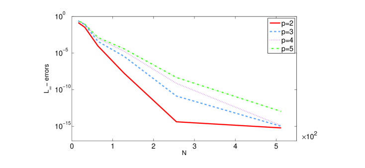
Figure 1: $L_{\infty}$-errors for the increasing values of $N$.

The question arises naturally how the solutions of the HBq equation behave when the coefficient of extra dispersion term $\eta_{2}\rightarrow 0^{+}$. For this aim, we perform some numerical tests for various values of $\eta_{2}$ and the fixed value $\eta_{1}=1$ for quadratic nonlinearity. We use the initial data

$$u(x,0)=A\,{\mbox{sech}}^{2}(\frac{1}{c}\sqrt{\frac{A}{6}}~{}x),$$ (6.1)

$$v(x,0)=2\,A\,{\mbox{sech}}^{2}\left(\frac{1}{c}\sqrt{\frac{A}{6}}~{}x\right)\,\tanh\left(\frac{1}{c}\sqrt{\frac{A}{6}}~{}x\right)$$ (6.2)

where $A=0.9$ and $c=\sqrt{\displaystyle\frac{2A}{3}+1}$. This initial data correspond to the initial profile of the exact solitary wave solution for the IBq equation given in [11]. In Figure 2, the solid line shows the exact solution of the improved Boussinesq equation which actually corresponds to the HBq equation with $\eta_{2}=0$. The dashed lines show the numerical solution of the HBq equation for the values of $\eta_{2}=10$, $\eta_{2}=5$, $\eta_{2}=1$ and $\eta_{2}=0.1$ and $\eta_{1}=1$. The problem is solved on the space interval $-100\leq x\leq 100$ for times up to $T=5$ where $N=512$ and $M=5000$. To observe the difference of two solutions more clear, this figure is presented on the space interval $-30\leq x\leq 30$. The numerical tests indicate that, as the parameter $\eta_{2}$ tends to zero, the solutions of the HBq equation converge to the solitary wave solution of the IBq equation.

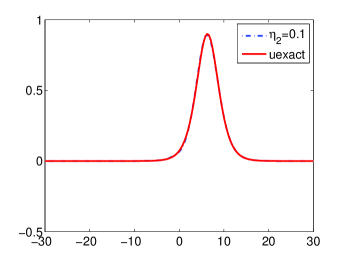
Figure 2: The numerical solution of the HBq equation for $\eta_{2}=10$, $\eta_{2}=5$, $\eta_{2}=1$, $\eta_{2}=0.1$ with $\eta_{1}=1$ and the exact solitary wave solution of the IBq equation

TABLE III

The amplitude at the final time $T=5$ with respect to changing $\eta_{2}$.

$\eta_{2}$	Amplitude ($p=2$)	Amplitude ($p=3$)
0.1	0.894	0.943
0.3	0.885	0.930
0.5	0.876	0.919
0.8	0.870	0.912
1	0.866	0.908

Table III shows the dependence of the amplitude to a changing $\eta_{2}$. In these experiments, we use the initial data (6.1)-(6.2) with $N=512$ and $M=5000$. We note that initial amplitude is $0.9$. From Table III, we can draw two observations:

(i) The amplitude of the wave is decreasing with increasing values of $\eta_{2}$. This numerical result agrees well with the fact that the wave spreads out with increasing dispersive effects.

(ii) The amplitude is increasing with increasing values of power of nonlinearity $p$. This numerical result is also agrees well with the fact that the wave steepens with increasing nonlinear effects.

6.2 Head-on Collision of Two Solitary Waves

In this section, we consider the HBq equation with quadratic nonlinearity and we study the head-on collision of two solitary waves with equal amplitudes. The initial conditions are given by

$$u(x,0)=\sum_{i=1}^{2}A{\mbox{sech}}^{4}(B(x-x_{0}^{i})),$$

$$v(x,0)=4\sum_{i=1}^{2}ABc_{i}{\mbox{sech}}^{4}\left(B(x-x_{0}^{i})\right)\,\tanh\left(B(x-x_{0}^{i})\right).$$

We consider two solitary waves, one initially located at $x_{0}^{1}=-40$ and moving to the right with amplitude $A$ ($c_{1}>0$) and one initially located at $x_{0}^{2}=40$ and moving to the left with amplitude $A$ ($c_{2}=-c_{1}$). The problem is solved again on the interval $-100\leq x\leq 100~{}$ for times up to $T=72$ using the Fourier pseudo-spectral method. All experiments in this section are performed for $N=512$ and $M=7200$. We first illustrate the head-on collision of two solitary waves with equal amplitudes $A\approx 0.39$ with $\eta_{1}=\eta_{2}=1$ and $A\approx 1.08$ with $\eta_{1}=\eta_{2}=2$ in Figure 3.

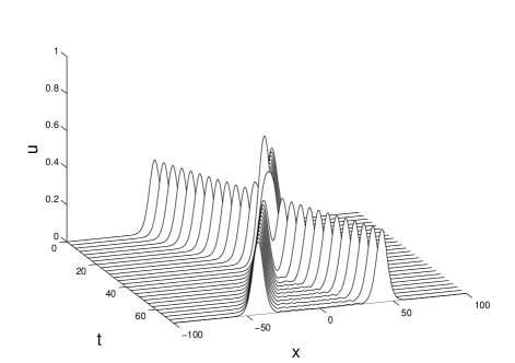
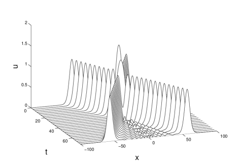
Figure 3: Surface plot of the head-on collision of two solitary waves with equal amplitudes. $A\approx 0.39$ (left panel) and $A\approx 1.08$ (right panel).

As the HBq equation cannot be solved by the inverse scattering method, the interaction of solitary waves are inelastic. Although secondary waves exist in all nonlinear interactions, they become more visible as we increase the amplitudes of the interacting waves.

Since an analytical solution is not available for the collision of two solitary waves, we cannot present the $L_{\infty}$-errors for this experiment. But, as a numerical check of the proposed Fourier pseudo-spectral scheme, we have observed the evolution of the change in the conserved quantity $I_{1}$. The error $\mid I_{1}(t)-I_{1}(0)\mid$ is approximately of order $10^{-14}$ and $10^{-10}$ for the amplitudes $A\approx 0.39$ and $A\approx 1.08$ up to the final time $T=72$, respectively. This behavior provides a valuable check on the numerical results.

6.3 Blow-up Solution

In the last section, we investigate the effect of extra dispersion term and the nonlinear term on the blow-up solutions of the HBq equation. The HBq equation is one of the class of nonlocal equation, we refer to Theorem $5.2$ in [10] as the blow-up criteria. Applied to the HBq equation, this theorem can be restated as:

Theorem 6.1.

Suppose $\phi=\Phi_{x},\psi=\Psi_{x}$ for some $\Phi,\Psi\in H^{2}(\Omega)$ and $F(\varphi)\in L^{1}(\Omega)$. If there are some $\mu>0$ such that

$$uf\left(u\right)\leq 2\mu u^{2}+2\left(1+2\mu\right)F\left(u\right)\mbox{ for all }u\in\mathbb{R},$$ (6.3)

and ${I_{3}}\left(0\right)<0~{}$, then the solution $u$ of the Cauchy problem for HBq equation with the initial conditions $u(x,0)=\phi(x)$, $u_{t}(x,0)=\psi(x)$ blows up in finite time.

First, we consider the HBq equation with both quadratic nonlinearity $f(u)=u^{2}$ and cubic nonlinearity $f(u)=-u^{3}$. We set the parameters $\eta_{1}=\eta_{2}=1$ in (1.3). For the quadratic nonlinearity, if we choose the initial data

$$\phi(x)=4\left(\frac{2x^{2}}{3}-1\right)e^{-\frac{~{}x^{2}}{3}},\hskip 30.0pt\psi(x)=\left(x^{2}-1\right)e^{-\frac{~{}x^{2}}{2}}$$ (6.4)

as in [15], and the condition (6.3) is satisfied for $\mu=\frac{1}{4}$. Similarly, for the cubic nonlinearity, the initial data are chosen as

$$\phi(x)=13\left(\frac{x^{2}}{2}-1\right)e^{-\frac{~{}x^{2}}{4}},\hskip 30.0pt\psi(x)=\left(1-x^{2}\right)e^{-\frac{~{}x^{2}}{2}}$$ (6.5)

where the inequality (6.3) is satisfied for $\mu=\frac{1}{2}$. We note that ${I_{3}}(0)<0$ for both cases. For the experiments in this section, the problem is solved on the interval $-10\leq x\leq 10$ up to final time $T=4$ for quadratic nonlinearity and $T=0.4$ for cubic nonlinearity.

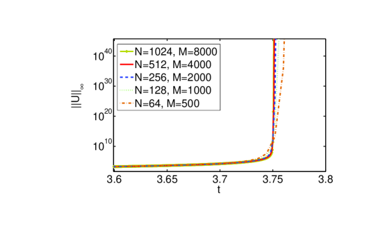
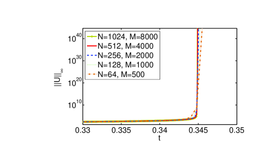
Figure 4: The variation of $\|U\|_{\infty}$ with time for increasingly refined discretization for quadratic nonlinearity (left panel) and cubic nonlinearity (right panel).

In order to check whether the numerical blow-up results are affected by the time and space step sizes, we now make some numerical experiments with varying resolutions. We start with the spatial and temporal resolutions corresponding to $N=64$ and $M=500$, respectively. Then we refine the mesh by increasing the number of both spatial and temporal grid points. We present the variation of the $L_{\infty}$-norm of the approximate solution obtained using the Fourier pseudo-spectral scheme for various mesh in Figure 4. To observe the blow-up profile more clear, figures are illustrated near the blow-up time. It is seen that curves converge to a limiting blow-up profile as the resolution is increased. For the number of spatial and temporal grid points more than $N=512$ and $M=4000$, the blow-up profile is not distinguishable from each other. Therefore, we set $N=512$ and $M=4000$ for the rest of the study. The numerical results strongly indicate that a blow-up is well underway by time $t=3.8$ for quadratic nonlinearity and $t=0.35$ for cubic nonlinearity. In Figure 5, we also illustrate the blow-up profile near the blow-up time at $t=3.710$, $t=3.711$, $t=3.7115$ and $t=3.712$ for the quadratic nonlinearity as in [16]. We observe that the $L_{\infty}$-norm of the blow-up solution increases very rapidly while the blow-up profile remains the same. Therefore, the blow-up appears to be a similarity type.

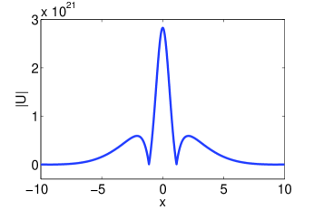
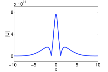
Figure 5: The blow-up profile of the HBq equation near the blow-up time at $t=3.710$, $t=3.711$, $t=3.7115$, $t=3.712$ for quadratic nonlinearity with $\eta_{1}=\eta_{2}=1$.

To investigate how the blow-up time depends on the coefficient of extra dispersion term $\eta_{2}$ with the fixed value $\eta_{1}=1$, we perform some numerical experiments. The variation of the blow-up time as $\eta_{2}\rightarrow 0^{+}$ is presented in Figure 6. As it is seen from the figure, less dispersion gives rise to earlier blow-up time.

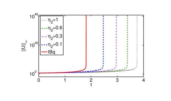
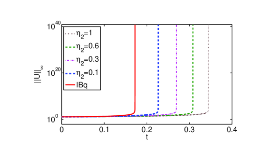
Figure 6: The variation of the blow-up time as $\eta_{2}\rightarrow 0^{+}$ for quadratic nonlinearity (left panel) and cubic nonlinearity (right panel).

To investigate how the blow-up time depends on the power $p$ of nonlinear term, we perform some numerical experiments. We use the initial data (6.4) for $f(u)=u^{p},~{}p=2,4,6$ and (6.5) for $f(u)=-u^{p},~{}p=3,5$. We set the parameters $\eta_{1}=\eta_{2}=1$ in (1.3). We note that it is possible to find some appropriate values for $\mu$ to satisfy the condition (6.3) for all these cases. Moreover, $I_{3}(0)$ also remains negative for increasing $p$ with the initial data (6.4) and (6.5). Figure 7 shows the blow-up time with respect to changing $p$. It can be observed that the blow-up time is decreasing with increasing powers of nonlinearity.

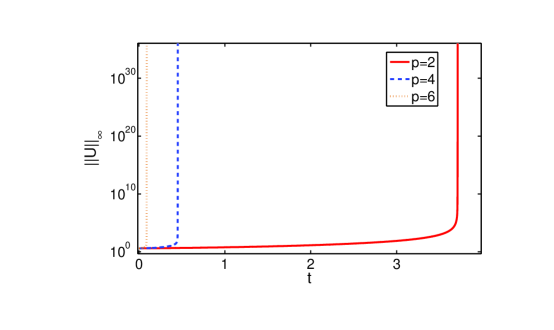
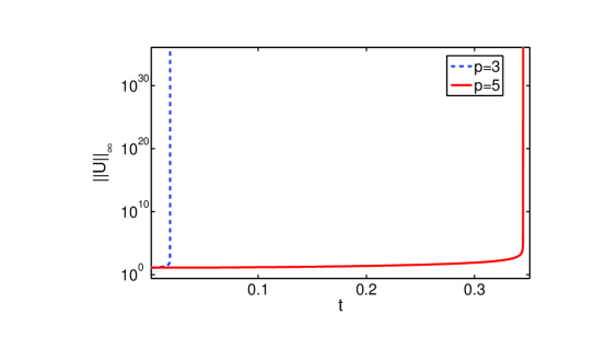
Figure 7: The blow-up time with respect to changing $p$.

Acknowledgement: This work has been supported by the Scientific and Technological Research Council of Turkey (TUBITAK) under the project MFAG-113F114. The authors gratefully acknowledge to the anonymous reviewers for the constructive comments and valuable suggestions which improved the first draft of paper.

References

- [1] J. Boussinesq, Théorie de l’intumescense liquide appelée onde solitaire ou de translation, se propageant dans un canal rectangulaire, C. R. Acad. Sci. Paris 72 (1871) 755–759.
- [2] J. Boussinesq, Théorie générale des mouvements, qui sont propagés dans un canal rectangulaire, C. R. Acad. Sci. Paris 73 (1871) 256–260.
- [3] J. Boussinesq, Théorie des ondes remous qui se propagent le long d’un canal rectangulaire horizontali en communiquant au liquide continu dans ce canal de vitesses sensiblement pareilles de la surface au fond, J. Math Pures Appl. 17 (1872) 55–108.
- [4] C. I. Christov, An energy-consistent dispersive shallow-water model, Wave Motion 1018 (2000) 1–14.
- [5] C. I. Christov, G. A. Maugin, A. V. Porubov, On boussinesq’s paradigm in nonlinear wave propagation, Comptes Rendus Mécanique 335 (9) (2007) 521–535.
- [6] I. L. Bogolubsky, Some examples of inelastic soliton interaction, Comput. Phys. Commun. 13 (1977) 149–155.
- [7] P. Rosenau, Dynamics of nonlinear mass-spring chains near the continuum limit, Physics Letters A 118 (5) (1986) 222 – 227.
- [8] P. Rosenau, Dynamics of dense discrete systems, Progr. Theoret. Phys. 79 (1988) 1028–1042.
- [9] N. Duruk, A. Erkip, H. A. Erbay, A higher-order Boussinesq equation in locally non-linear theory of one-dimensional non-local elasticity, IMA J. Appl. Math. 74 (2009) 97–106.
- [10] N. Duruk, H. A. Erbay, A. Erkip, Global existence and blow-up for a class of nonlocal nonlinear cauchy problems arising in elasticity, Nonlinearity 23 (2010) 107–118.
- [11] H. Borluk, G. M. Muslu, A Fourier pseudospectral method for a generalized improved Boussinesq equation, Numerical Methods for Partial Differential Equations 31 (2015) 995–1008.
- [12] C. Canuto, A. Quarteroni, Approximation results for orthogonal polynomials in sobolev spaces, Mathematics of Computation 38 (1982) 67–86.
- [13] A. Rashid, S. Akram, Convergence of fourier spectral method for resonant long-short nonlinear wave interaction, Applications of Mathematics 55 (2010) 337–350.
- [14] T. Runst, W. Sickel, Sobolev spaces of fractional order, Nemytskij operators, and nonlinear partial differential equations, vol. 3, Walter de Gruyter, 1996.
- [15] A. Godefroy, Blow-up solutions of a generalized Boussinesq equation, IMA J. Numer. Anal. 60 (1998) 122–138.
- [16] J. L. Bona, H. Kalisch, Singularity formation in the generalized Benjamin-Ono Equation, Discrete and Continuous Dynamical Systems 11 (2004) 27–45.