A superharmonic vector for a nonnegative matrix with QBD block structure and its application to a Markov modulated two dimensional reflecting process

Abstract

Markov modulation is versatile in generalization for making a simple stochastic model which is often analytically tractable to be more flexible in application. In this spirit, we modulate a two dimensional reflecting skip-free random walk in such a way that its state transitions in the boundary faces and interior of a nonnegative integer quadrant are controlled by Markov chains. This Markov modulated model is referred to as a 2d-QBD process according to Ozawa [36]. We are interested in the tail asymptotics of its stationary distribution, which has been well studied when there is no Markov modulation.

Ozawa studied this tail asymptotics problem, but his answer is not analytically tractable. We think this is because Markov modulation is so free to change a model even if the state space for Markov modulation is finite. Thus, some structure, say, extra conditions, would be needed to make the Markov modulation analytically tractable while minimizing its limitation in application.

The aim of this paper is to investigate such structure for the tail asymptotic problem. For this, we study the existence of a right subinvariant positive vector, called a superharmonic vector, of a nonnegative matrix with QBD block structure, where each block matrix is finite dimensional. We characterize this existence under a certain extra assumption. We apply this characterization to the 2d-QBD process, and derive the tail decay rates of its marginal stationary distribution in an arbitrary direction. This solves the tail decay rate problem for a two node generalized Jackson network, which has been open for many years.

Keywords: Subinvariant vector, QBD structured matrix, Markov modulation, two dimensional reflecting random walk, generalized Jackson network, stationary distribution, large deviations.

1 Introduction

Our primary interest is in methodology for deriving the tail asymptotics of the stationary distribution of a Markov modulated two dimensional reflecting random walk for queueing network applications, provided it is stable. This process has two components, front and background processes. We assume that the front process is a skip-free reflecting random walk on a nonnegative quarter plane of lattice, and the background process has finitely many states. We are particularly interested in a two node generalized Jackson network for its application.

According to Ozawa [36], we assume the following transition structure. The state space of the front process is composed of the inside of the quarter plane and three boundary faces, the origin and the two half coordinate axes. Within each region, state-transitions are homogeneous, that is, subject to a Markov modulated random walk, but different regions may have different state-transitions. Between pairs of the four regions, state-transitions may also be different. See Figure 1 in Section 3.1 for their details. This Markov modulated two dimensional random walk is called a discrete-time 2d-QBD process, 2d-QBD process for short, in [36]. We adopt the same terminology. This process is flexible enough to handle many two node queueing networks in continuous time through uniformization. The generalized Jackson network is such an example.

For the 2d-QBD process, we assume that it has a stationary distribution, and denote a random vector subject to it by $({\boldsymbol{L}},J)$, where ${\boldsymbol{L}}$ represents a random walk component taking values in $\mathbb{R}_{+}^{2}$ while $J$ represents a background state. For $i=1,2$, we consider the tail asymptotics by logarithmic ratios of the stationary tail probabilities in the $i$-th coordinate directions:

$$\frac{1}{n}\log\mathbb{P}(L_{i}>n,L_{3-i}=\ell,J=k),\qquad n\to\infty,$$ (1.1)

for each fixed $\ell\geq 0$ and background state $k$, and those of the marginal stationary distribution in an arbitrary direction ${\boldsymbol{c}}\equiv(c_{1},c_{2})$:

$$\frac{1}{x}\log\mathbb{P}(c_{1}L_{1}+c_{2}L_{2}>x),\qquad x\to\infty.$$ (1.2)

It will be shown that those ratios converges to constants (Theorems 3.2 and 3.3). They are negative, and their absolute values are called exponential decay rates. We demonstrate those tail asymptotic results for a two node generalized Jackson network with Markov modulated arrivals and phase type service time distributions. This solves the problem which has been open for many years (see Section 4.2 for details).

Ozawa [36] studied the tail asymptotics in the coordinate directions including (1.1). He showed that the method for a two-dimensional reflecting random walk studied by Miyazawa [27] is applicable with help of invariant vectors obtained by Li and Zhao [24]. We refer to this method as a QBD approach, which is composed of the following three key steps.

• Formulate the 2d-QBD process as a one dimensional QBD process with infinitely many background states, where one of the coordinate axes is taken as a level.

• Find right and left invariant vectors of a nonnegative matrix with QBD block structure, which will be introduced shortly, and get upper and lower bounds of the tail decay rates.

• Derive the tail decay rates, combining those results in the two directions.

Here, an infinite dimensional square matrix is said to have QBD block structure if it is partitioned into blocks in such a way that each block is a square matrix of the same size except for the first row and first column blocks, the whole matrix is block tridiagonal and each row of blocks is repeated and shifted except for the first two rows (see (2.5) for its definite form). In step 1), the blocks for the one dimensional QBD are infinite dimensional, while, in step 2), those for the nonnegative matrix are finite dimensional.

A hard part of this QBD approach is in step 2). In [36], the invariant vectors are only obtained by numerically solving certain parametrized equations over a certain region of parameters. This much degrades applicability of the tail asymptotic results. For example, it is hard to get useful information from them for the tail asymptotics in the two node generalized Jackson network (see, e.g, [12, 15]). We think this analytic intractability can not be avoided because no structural condition is assumed for the Markov modulation. In applications, it may have certain structure. Thus, it is interesting to find conditions for the invariant vectors to be analytically tractable while minimizing limitations in application.

Another problem in [36] is complicated descriptions. They can not be avoided because of the complicated modeling structure, but we easily get lost in computations. We think here simplification or certain abstraction is needed.

In addition to those two problems, the QBD approach is not so useful to study the tail asymptotics in an arbitrary direction. For this, it is known that the stationary inequalities in terms of moment generating functions are useful in the case that there is no Markov modulation (e.g., see [19, 28]). So far, it is interesting to see whether this moment generating function approach still works under Markov modulation.

We attack those three problems in this paper. We first consider the description problem, and find a simpler matrix representation for a nonnegative matrix with QBD block structure. This representation is referred to as a canonical form. We then consider the problem in step 2).

For this, we relax the problem by considering a right subinvariant positive vector, which is said to be superharmonic, instead of a right invariant positive vector, which is said to be harmonic. It is known that the existence of a right subinvariant vector is equivalent to that of a left subinvariant nonnegative vector (e.g., see [40]). When a nonnegative matrix is stochastic, a right subinvariant vector can be viewed as a superharmonic function. Because of this fact, we use the terminology superharmonic vector. In the stochastic case, it obviously exists. When the matrix is substochastic and does not have the boundary blocks, this problem has been considered in studying a quasi-stationary distribution for QBD processes (see, e.g., [17, 23, 24]).

In step 2), we do not assume any stochastic or substochastic condition for a nonnegative matrix with QBD block structure, which is crucial in our applications. As we will see, we can find necessary and sufficient conditions for such a matrix to have a superharmonic vector (see Theorem 2.1). The sufficiency is essentially due to Li and Zhao [24] and related to Bean et al. [2] (see Remarks 2.1 and 2.2). However, this characterization is not useful in application as we already discussed. So, we will assume a certain extra condition to make an answer to be tractable. Under this extra assumption, we characterize the existence of a superharmonic vector using primitive data on the block matrices (Theorem 2.2).

This characterization enables us to derive the tail asymptotics of the stationary distribution in the coordinate directions for the 2d-QBD process. For the problem of the tail asymptotics in an arbitrary direction, we show that the moment generating function approach can be extended for the Markov modulated case. For this, we introduce a canonical form for the Markov modulated two dimensional random walk, which is similar to that for a nonnegative matrix with QBD block structure.

There has been a lot work on tail asymptotic problems in queueing networks (see, e.g., [28] and references therein). Most of studies focus on two dimensional reflecting processes or two node queueing networks. The 2d-QBD process belongs to this class of models, but allows them to have background processes with finitely many states. There is a huge gap between finite and infinite numbers of background states, but we hope the present results will stimulate to study higher dimensional tail asymptotic problems.

This paper is made up by five sections and appendices. Section 2 drives necessary and sufficient conditions for a nonnegative matrix with QBD block structure to have a right sub-invariant vector with and without extra assumptions. This result is applied to the 2d-QBD process, and the tail decay rates of its stationary distribution are derived in Section 3. The tail decay rates of the marginal stationary distribution in an arbitrary direction are obtained for the generalized Jackson network in Section 4. We finally give some concluding remarks in Section 5.

We summarize basic notation which will be used in this paper (see Tables 1 and 2).

$\mathbb{Z}$	the set of all integers,	$\mathbb{Z}_{+}$	the set of all nonnegative integers,
$\mathbb{R}$	the set of all real numbers,	$\mathbb{R}_{+}$	the set of all nonnegative real numbers,
$\mathbb{H}$	$\{-1,0,1\}$,	$\mathbb{H}_{+}$	$\{0,1\}$,
$\langle{\boldsymbol{x}},{\boldsymbol{y}}\rangle$	$x_{1}y_{1}+x_{2}y_{2}$ for ${\boldsymbol{x}},{\boldsymbol{y}}\in\mathbb{R}^{2}$,	${\boldsymbol{1}}$	the column vector whose entries are all units.

Table 1: Notation for sets of numbers and vectors

For nonnegative square matrices $T,T_{i},T_{ij}$ with indices $i,j\in\mathbb{Z}$ such that $T_{i}$ and $T_{ij}$ are null matrices except for finitely many $i$ and $j$, we will use the following conventions.

$c_{p}(T)$	$\sup\{u\geq 0;\sum_{n=0}^{\infty}u^{n}T^{n}<\infty\}$: the convergence parameter of $T$,
$\gamma_{{\mbox{\scriptsize\sc pf}}}(T)$	the Perron-Frobenius eigenvalue of $T$ if $T$ is finite dimensional,
	while it equals $c_{p}(T)^{-1}$ if $T$ is infinite dimensional.
$T_{*}(\theta)$	$\sum_{i\in\mathbb{Z}}e^{i\theta}T_{i}$ for $\theta\in\mathbb{R}$: the matrix MGF of $\{T_{i}\}$,
	where MGF is for moment generating function,
$T_{**}({\boldsymbol{\theta}})$	$\sum_{i,j\in\mathbb{Z}}e^{(i,j){\boldsymbol{\theta}}}T_{ij}$ for ${\boldsymbol{\theta}}\in\mathbb{R}^{2}$: the matrix MGF of $\{T_{ij}\}$,
$\gamma^{(\cdot)}(\cdot)$	$\gamma^{(T_{*})}(\theta)=\gamma_{{\mbox{\scriptsize\sc pf}}}(T_{*}(\theta))$, $\quad\gamma^{(T_{**})}({\boldsymbol{\theta}})=\gamma_{{\mbox{\scriptsize\sc pf}}}(T_{**}({\boldsymbol{\theta}}))$,
$(I-T)^{-1}$	$\sum_{n=0}^{\infty}T^{n}$ (this is infinite if $c_{p}(T)<1$),
$\Delta_{{\boldsymbol{x}}}$	the diagonal matrix whose $i$-th diagonal entry is $x_{i}$,
	where $x_{i}$ is the $i$-th entry of vector ${\boldsymbol{x}}$.

Table 2: Conventions for matrices and their MGF

Here, the sizes of those matrices must be the same among those with the same type of indices, but they may be infinite. We also will use those matrices and related notation when the off-diagonal entries of $T,T_{i},T_{ij}$ are nonnegative.

2 Nonnegative matrices and QBD block structure

Let $K$ be a nonnegative square matrix with infinite dimension. Throughout this section, we assume the following regularity condition.

• $K$ is irreducible, that is, for each entry $(i,j)$ of $K$, there is some $n\geq 1$ such that the $(i,j)$ entry of $K^{n}$ is positive.

2.1 Superharmonic vector

In this subsection, we do not assume any assumption other than (2a), and introduce some basic notions. A positive column vector ${\boldsymbol{y}}$ satisfying

$$K{\boldsymbol{y}}\leq{\boldsymbol{y}}$$ (2.1)

is called a superharmonic vector of $K$, where the inequality of vectors is entry-wise. The condition (2.1) is equivalent to that there exists a positive row vector ${\boldsymbol{x}}$ satisfying ${\boldsymbol{x}}K\leq{\boldsymbol{x}}$. This ${\boldsymbol{x}}$ is called a sub-invariant vector. Instead of (2.1), if, for $u>0$,

$$uK{\boldsymbol{y}}\leq{\boldsymbol{y}},$$ (2.2)

then ${\boldsymbol{y}}$ is called a $u$-superharmonic vector. We will not consider this vector, but most of our arguments are parallel to those for a superharmonic vector because ${\boldsymbol{y}}$ of (2.2) is superharmonic for $uK$.

These conditions can be given in terms of the convergence parameter $c_{p}(K)$ of $K$ (see Table 2 for its definition). As shown in Chapter 5 of the book of Nummelin [34] (see also Chapter 6 of [38]),

$$c_{p}(K)=\sup\{u\geq 0;uK{\boldsymbol{y}}\leq{\boldsymbol{y}}\mbox{ for some }{\boldsymbol{y}}>0\},$$ (2.3)

or equivalently $c_{p}(K)=\sup\{u\geq 0;u{\boldsymbol{x}}K\leq{\boldsymbol{x}}\mbox{ for some }{\boldsymbol{x}}>0\}$. Applying this fact to $K$, we have the following lemma. For completeness, we give its proof.

Lemma 2.1

A nonnegative matrix $K$ satisfying (2a) has a superharmonic vector if and only if $c_{p}(K)\geq 1$.

Proof. If $K$ has a superharmonic vector, then we obviously have $c_{p}(K)\geq 1$ by (2.3). Conversely, suppose $c_{p}(K)\geq 1$. Then, by (2.3), for any positive $u<1$, we can find a positive vector ${\boldsymbol{z}}(u)$ such that

$$uK{\boldsymbol{z}}(u)\leq{\boldsymbol{z}}(u).$$ (2.4)

Denote the $i$-th entry of ${\boldsymbol{z}}(u)$ by $z_{i}(u)$, and define vector ${\boldsymbol{y}}(u)$ whose $i$-th entry $y_{i}(u)$ is given by

$$y_{i}(u)=\min(1,z_{i}(u)/z_{0}(u)).$$

Then, it follows from (2.4) that $y_{0}(u)=1$, $y_{i}(u)\leq 1$ for all $i$, and

$$uK{\boldsymbol{y}}(u)\leq{\boldsymbol{y}}(u).$$

Taking the limit infimum of both sides of the above inequality as $u\uparrow 1$, and letting ${\boldsymbol{y}}=\liminf_{u\uparrow 1}{\boldsymbol{y}}(u)$, we have (2.1). Thus, $K$ indeed has a superharmonic vector ${\boldsymbol{y}}$, which must be positive by the irreducible assumption (2a).

The importance of Condition (2.1) lies in the fact that $\Delta_{{\boldsymbol{y}}}^{-1}K\Delta_{{\boldsymbol{y}}}$ is substochastic, that is, $K$ can be essentially considered as a substochastic matrix. This enables us to use probabilistic arguments for manipulating $K$ in computations.

2.2 QBD block structure and its canonical form

We now assume further structure for $K$. Let $m_{0}$ and $m$ be arbitrarily given positive integers. Let $A_{i}$ and $B_{i}$ for $i=-1,0,1$ be nonnegative matrices such that $A_{i}$ for $i=-1,0,1$ are $m\times m$ matrices, $B_{-1}$ is an $m_{0}\times m$ matrix, $B_{0}$ is an $m_{0}\times m_{0}$ matrix and $B_{1}$ is $m\times m_{0}$ matrix. We assume that $K$ has the following form:

$$K=\left(\begin{matrix}B_{0}&B_{1}&0&0&0&\cdots\cr B_{-1}&A_{0}&A_{1}&0&0&\cdots\cr 0&A_{-1}&A_{0}&A_{1}&0&\cdots\cr 0&0&A_{-1}&A_{0}&A_{1}&\cdots\cr&\ddots&\ddots&\ddots&\ddots&\cdots\cr\end{matrix}\right).$$ (2.5)

If $K$ is stochastic, then it is the transition matrix of a discrete-time QBD process. Thus, we refer to $K$ of (2.5) as a nonnegative matrix with QBD block structure.

As we discussed in Section 1, we are primarily interested in tractable conditions for $K$ to have a superharmonic vector. Denote this vector by ${\boldsymbol{y}}\equiv({\boldsymbol{y}}_{0},{\boldsymbol{y}}_{1},\ldots)^{{\mbox{\scriptsize\sc t}}}$. That is, ${\boldsymbol{y}}$ is positive and satisfies the following inequalities.

$$B_{0}{\boldsymbol{y}}_{0}+B_{1}{\boldsymbol{y}}_{1}\leq{\boldsymbol{y}}_{0},$$ (2.6)

$$B_{-1}{\boldsymbol{y}}_{0}+A_{0}{\boldsymbol{y}}_{1}+A_{1}{\boldsymbol{y}}_{2}\leq{\boldsymbol{y}}_{1},$$ (2.7)

$$A_{-1}{\boldsymbol{y}}_{n-1}+A_{0}{\boldsymbol{y}}_{n}+A_{1}{\boldsymbol{y}}_{n+1}\leq{\boldsymbol{y}}_{n},\qquad n=2,\ldots.$$ (2.8)

Although the QBD block structure is natural in applications, there are two extra equations (2.6) and (2.7) which involve the boundary blocks $B_{i}$. Let us consider how to reduce them to one equation. From (2.6), $B_{0}{\boldsymbol{y}}_{0}\leq{\boldsymbol{y}}_{0}$ and $B_{0}{\boldsymbol{y}}_{0}\neq{\boldsymbol{y}}_{0}$. Hence, if $c_{p}(B_{0})=1$, then ${\boldsymbol{y}}_{0}$ must be the left invariant vector of $B_{0}$ (see Theorem 6.2 of [38]), but this is impossible because ${\boldsymbol{y}}_{1}>{\boldsymbol{0}}$. Thus, we must have $c_{p}(B_{0})>1$, and therefore $(I-B_{0})^{-1}$ is finite (see our convention (Table 2) for this inverse). Let

$$C_{0}=B_{-1}(I-B_{0})^{-1}B_{1}+A_{0},$$ (2.9)

then (2.6) and (2.7) yield

$$C_{0}{\boldsymbol{y}}_{1}+A_{1}{\boldsymbol{y}}_{2}\leq{\boldsymbol{y}}_{1}.$$ (2.10)

This suggests that we should define a matrix $\overline{K}$ as

$$\overline{K}=\left(\begin{matrix}C_{0}&A_{1}&0&0&0&\cdots\cr A_{-1}&A_{0}&A_{1}&0&0&\cdots\cr 0&A_{-1}&A_{0}&A_{1}&0&\cdots\cr 0&0&A_{-1}&A_{0}&A_{1}&\cdots\cr&\ddots&\ddots&\ddots&\ddots&\ddots\cr\end{matrix}\right),$$ (2.11)

where $C_{0}$ is defined by (2.9). Denote the principal matrix of $K$ (equivalently, $\overline{K}$) obtained by removing the first row and column blocks by $K_{+}$. Namely,

$$K_{+}=\left(\begin{matrix}A_{0}&A_{1}&0&0&\cdots\cr A_{-1}&A_{0}&A_{1}&0&\cdots\cr 0&A_{-1}&A_{0}&A_{1}&\cdots\cr&\ddots&\ddots&\ddots&\ddots\cr\end{matrix}\right).$$ (2.12)

Lemma 2.2

(a) $K$ has a superharmonic vector if and only if $\overline{K}$ has a superharmonic vector. (b) $\max(c_{p}(K),c_{p}(\overline{K}))\leq c_{p}(K_{+})$. (c) If $c_{p}(K)\geq 1$, then $c_{p}(K)\leq c_{p}(\overline{K})\leq c_{p}(K_{+})$.

Remark 2.1

A similar result for $K$ and $K_{+}$ is obtained in Bean et al. [2].

Proof. Assume that $K$ has a superharmonic vector ${\boldsymbol{y}}\equiv({\boldsymbol{y}}_{0},{\boldsymbol{y}}_{1},\ldots)^{{\mbox{\scriptsize\sc t}}}$. Then, we have seen that $c_{p}(B_{0})>1$, and therefore $(I-B_{0})^{-1}<\infty$. Define $\overline{{\boldsymbol{y}}}\equiv(\overline{{\boldsymbol{y}}}_{0},\overline{{\boldsymbol{y}}}_{1},\ldots)^{{\mbox{\scriptsize\sc t}}}$ by $\overline{{\boldsymbol{y}}}_{n}={\boldsymbol{y}}_{n+1}$ for $n\geq 0$, and define $C_{0}$ by (2.9). Then, from (2.10) , we have

$$C_{0}\overline{{\boldsymbol{y}}}_{0}+A_{1}\overline{{\boldsymbol{y}}}_{1}\leq\overline{{\boldsymbol{y}}}_{0}.$$

This and (2.8) verify that $\overline{{\boldsymbol{y}}}$ is superharmonic for $\overline{K}$. On the contrary, assume that $\overline{K}$ is well defined and $\overline{{\boldsymbol{y}}}\equiv(\overline{{\boldsymbol{y}}}_{0},\overline{{\boldsymbol{y}}}_{1},\ldots)^{{\mbox{\scriptsize\sc t}}}$ is superharmonic for $\overline{K}$. Obviously, the finiteness of $\overline{K}$ implies that $B_{-1}(I-B_{0})^{-1}B_{1}$ is finite. Suppose that $c_{p}(B_{0})\leq 1$, then some principal submatrix of $(I-B_{0})^{-1}$ has divergent entries in every row and column of this submatrix. Denote a collection of all such principal matrices which are maximal in their size by ${\cal P}_{0}$. Then, all entries $(i,j)$ of submatrices in ${\cal P}_{0}$, we must have, for all $n\geq 0$,

$$[B_{-1}]_{ki}\left[\sum_{s=0}^{n}B_{0}^{s}\right]_{ij}[B_{1}]_{j\ell}=0,\qquad\forall k,\ell\in\{1,2,\ldots,m\},$$

because of the finiteness of $B_{-1}(I-B_{0})^{-1}B_{1}$. This contradicts the irreducibility (2a) of $K$. Hence, we have $c_{p}(B_{0})>1$. Define ${\boldsymbol{y}}\equiv({\boldsymbol{y}}_{0},{\boldsymbol{y}}_{1},\ldots)^{{\mbox{\scriptsize\sc t}}}$ as

$${\boldsymbol{y}}_{0}=(I-B_{0})^{-1}B_{1}\overline{{\boldsymbol{y}}}_{0},\qquad{\boldsymbol{y}}_{n}=\overline{{\boldsymbol{y}}}_{n-1},\quad n\geq 1,$$

where $(I-B_{0})^{-1}<\infty$ because of $c_{p}(B_{0})>1$. Then, from (2.9), we have

$$C_{0}{\boldsymbol{y}}_{1}=C_{0}\overline{{\boldsymbol{y}}}_{0}=B_{-1}{\boldsymbol{y}}_{0}+A_{0}{\boldsymbol{y}}_{1},$$

and therefore the fact that $C_{0}\overline{{\boldsymbol{y}}}_{0}+A_{1}\overline{{\boldsymbol{y}_{1}}}\leq\overline{{\boldsymbol{y}}}_{0}$ implies (2.7). Finally, the definition of ${\boldsymbol{y}}_{0}$ implies (2.6) with equality, while the definition of ${\boldsymbol{y}}_{n}$ for $n\geq 1$ implies (2.8). Hence, ${\boldsymbol{y}}$ is superharmonic for $K$. This proves (a). (b) is immediate from (2.3) since $({\boldsymbol{y}}_{1},\ldots)^{{\mbox{\scriptsize\sc t}}}$ is superharmonic for $K_{+}$ if $({\boldsymbol{y}}_{0},{\boldsymbol{y}}_{1},\ldots)^{{\mbox{\scriptsize\sc t}}}$ is superharmonic for $K$ (or $\overline{K}$). For (c), recall that the canonical form of $uK$ is denoted by $\overline{uK}$ for $u>0$. If $u\geq 1$, we can see that $u\overline{K}\leq\overline{uK}$, and therefore $c_{p}(K)\leq c_{p}(\overline{K})$. This and (b) conclude (c).

By this lemma, we can work on $\overline{K}$ instead of $K$ so as to find a superharmonic vector. It is notable that all block matrices of $\overline{K}$ are $m\times m$ square matrices and it has repeated row and column structure except for the first row and first column blocks. This greatly simplifies computations. So far, we refer to $\overline{K}$ as the canonical form of $K$.

In what follows, we will mainly work on the canonical form $\overline{K}$ of $K$. For simplicity, we will use ${\boldsymbol{y}}\equiv({\boldsymbol{y}}_{0},{\boldsymbol{y}}_{1},\ldots)^{{\mbox{\scriptsize\sc t}}}$ for a superharmonic vector of $\overline{K}$.

2.3 Existence of a superharmonic vector

Suppose that $\overline{K}$ of (2.11) has a superharmonic vector ${\boldsymbol{y}}\equiv({\boldsymbol{y}}_{0},{\boldsymbol{y}}_{1},\ldots)^{{\mbox{\scriptsize\sc t}}}$. That is,

$$C_{0}{\boldsymbol{y}}_{0}+A_{1}{\boldsymbol{y}}_{1}\leq{\boldsymbol{y}}_{0},$$ (2.13)

$$A_{-1}{\boldsymbol{y}}_{n-1}+A_{0}{\boldsymbol{y}}_{n}+A_{1}{\boldsymbol{y}}_{n+1}\leq{\boldsymbol{y}}_{n},\qquad n\geq 1.$$ (2.14)

In this section, we consider conditions for the existence of a superharmonic vector.

Letting $C_{1}=A_{1}$, we recall matrix moment generating functions for $\{A_{i}\}$ and $\{C_{i}\}$ (see Table 2):

$$A_{*}(\theta)=e^{-\theta}A_{-1}+A_{0}+e^{\theta}A_{1},\qquad C_{*}(\theta)=C_{0}+e^{\theta}C_{1},\qquad\theta\in\mathbb{R}.$$

From now on, we always assume a further irreducibility in addition to (2a).

• $A_{*}(0)$ is irreducible.

Since $A_{*}(\theta)$ and $C_{*}(\theta)$ are nonnegative and finite dimensional square matrices, they have Perron-Frobenius eigenvalues $\gamma^{(A_{*})}(\theta)(\equiv\gamma_{{\mbox{\scriptsize\sc pf}}}(A_{*}(\theta)))$ and $\gamma^{(C_{*})}(\theta)(\equiv\gamma_{{\mbox{\scriptsize\sc pf}}}(C_{*}(\theta)))$, respectively, and their right eigenvectors ${\boldsymbol{h}}^{(A_{*})}(\theta)$ and ${\boldsymbol{h}}^{(C_{*})}(\theta)$, respectively. That is,

$$A_{*}(\theta){\boldsymbol{h}}^{(A_{*})}(\theta)=\gamma^{(A_{*})}(\theta){\boldsymbol{h}}^{(A_{*})}(\theta),$$ (2.15)

$$C_{*}(\theta){\boldsymbol{h}}^{(C_{*})}(\theta)=\gamma^{(C_{*})}(\theta){\boldsymbol{h}}^{(C_{*})}(\theta),$$ (2.16)

where $C_{*}(\theta)$ may not be irreducible, so we take a maximal eigenvalue among those which have positive right invariant vectors. Thus, ${\boldsymbol{h}}^{(A_{*})}(\theta)$ is positive, but ${\boldsymbol{h}}^{(C_{*})}(\theta)$ is nonnegative with possibly zero entries. These eigenvectors are unique up to constant multipliers.

It is well known the $\gamma^{(A_{*})}(\theta)$ and $\gamma^{(C_{*})}(\theta)$ are convex functions of $\theta$ (see, e.g., Lemma 3.7 of [32]). Furthermore, their reciprocals are the convergence parameters of $A_{*}(\theta)$ and $C_{*}(\theta)$, respectively. It follows from the convexity of $\gamma^{(A_{*})}(\theta)$ and the fact that some entries of $A_{*}(\theta)$ diverge as $|\theta|\to\infty$ that

$$\lim_{\theta\to-\infty}\gamma^{(A_{*})}(\theta)=\lim_{\theta\to+\infty}\gamma^{(A_{*})}(\theta)=+\infty.$$ (2.17)

We introduce the following notation.

$$\Gamma^{(1d)}_{+}=\{\theta\in\mathbb{R};\gamma^{(A_{*})}(\theta)\leq 1\},\qquad\Gamma^{(1d)}_{0}=\{\theta\in\mathbb{R};\gamma^{(C_{*})}(\theta)\leq 1\},$$

where $\Gamma^{(1d)}_{0}\not=\emptyset$ implies that $C_{0}$ is finite, that is, $c_{p}(B_{0})>1$. By (2.17), $\Gamma^{(1d)}_{+}$ is a bounded interval or the empty set.

In our arguments, we often change the repeated row of blocks of $K$ and $\overline{K}$ so that they are substochastic. For this, we introduce the following notation. For each $\theta\in\mathbb{R}$ and ${\boldsymbol{h}}^{(A_{*})}(\theta)$ determined by (2.15), let

$$\widehat{A}^{(\theta)}_{\ell}=e^{\theta\ell}\Delta_{{\boldsymbol{h}}^{(A_{*})}(\theta)}^{-1}A_{\ell}\Delta_{{\boldsymbol{h}}^{(A_{*})}(\theta)},\qquad\ell=0,\pm 1,$$

where we recall that $\Delta_{{\boldsymbol{a}}}$ is the diagonal matrix whose diagonal entry is given by the same dimensional vector ${\boldsymbol{a}}$. Let

$$\widehat{A}^{(\theta)}=\widehat{A}^{(\theta)}_{-1}+\widehat{A}^{(\theta)}_{0}+\widehat{A}^{(\theta)}_{1}.$$

Note that $\widehat{A}^{(\theta)}=\Delta_{{\boldsymbol{h}}^{(A_{*})}(\theta)}^{-1}A_{*}(\theta)\Delta_{{\boldsymbol{h}}^{(A_{*})}(\theta)}$, and therefore $\widehat{A}^{(\theta)}{\boldsymbol{1}}=\gamma^{(A_{*})}(\theta){\boldsymbol{1}}$.

The following lemma is the first step in characterizing $c_{p}(K)\geq 1$.

Lemma 2.3

(a) $c_{p}(K_{+})\geq 1$ if and only if $\Gamma^{(1d)}_{+}\neq\emptyset$, and therefore $c_{p}(K)\geq 1$ implies $\Gamma^{(1d)}_{+}\neq\emptyset$. (b) $c_{p}(K_{+})=(\min\{\gamma^{A_{*}}(\theta);\theta\in\mathbb{R}\})^{-1}$.

This lemma may be considered to be a straightforward extension of Theorem 2.1 of Kijima [17] from a substochastic to a nonnegative matrix. So, it may be proved similarly, but we give a different proof in Appendix A. There are two reasons for this. First, it makes this paper selfcontained. Second, we wish to demonstrate that it is hard to remove the finiteness of $m$ on block matrices.

We now present necessary and sufficient conditions for $\overline{K}$, equivalently $K$, to have a superharmonic vector.

Theorem 2.1

(a) If $\Gamma^{(1d)}_{+}\neq\emptyset$, then $N\equiv(I-K_{+})^{-1}$ is finite, and therefore $G_{-}\equiv N_{11}A_{-1}$ is well defined and finite, where $N_{11}$ is the $(1,1)$-entry of $N$. (b) $c_{p}(\overline{K})\geq 1$ holds if and only if $\Gamma^{(1d)}_{+}\neq\emptyset$ and

$$\gamma_{{\mbox{\scriptsize\sc pf}}}(C_{0}+A_{1}G_{-})\leq 1.$$ (2.18)

If the equality holds in (2.18), then $c_{p}(\overline{K})=1$.

Remark 2.2

The sufficiency in (b) is essentially obtained in Theorem 6 of [24], which is used in Sections 3.4 and 3.5 of [36], where the eigenvalue $\gamma_{{\mbox{\scriptsize\sc pf}}}(C_{0}+A_{1}G_{-})$ corresponds to $u_{0}(1)$ in [24]. We do not need the function $u_{0}(\beta)$ there because we work on a nonnegative matrix while substochasticity is assumed in [24].

Proof. (a) Assume that $\theta\in\Gamma^{(1d)}_{+}\neq\emptyset$, then we can find a $\theta_{1}$ such that $\theta_{1}=\arg_{\theta}\min\{\theta\in\mathbb{R};\gamma^{A_{*}}(\theta)=1\}$. For this $\theta_{1}$, let ${\boldsymbol{y}}(\theta_{1})=({\boldsymbol{h}}^{(A_{*})}(\theta_{1}),e^{\theta_{1}}{\boldsymbol{h}}^{(A_{*})}(\theta_{1}),\ldots)^{{\mbox{\scriptsize\sc t}}}$, and let

$$\breve{K}_{+}^{(\theta_{1})}=\Delta_{{\boldsymbol{y}}(\theta_{1})}^{-1}K_{+}\Delta_{{\boldsymbol{y}}(\theta_{1})}.$$

It is easy to see that $\breve{K}_{+}^{(\theta_{1})}$ is strictly substochastic because the first row of blocks is defective. Hence, $(1-\breve{K}_{+}^{(\theta_{1})})^{-1}$ must be finite, and therefore $(I-K_{+})^{-1}$ is also finite. This proves (a).
(b) Assume that $c_{p}(\overline{K})\geq 1$, then $\Gamma^{(1d)}_{+}\neq\emptyset$ by Lemma 2.3. Hence, $(I-K_{+})^{-1}$ is finite by (a). Because of $c_{p}(\overline{K})\geq 1$, $\overline{K}$ has a superharmonic vector. We denote this vector by ${\boldsymbol{y}}=\{{\boldsymbol{y}}_{n};n=0,1,\ldots\}^{{\mbox{\scriptsize\sc t}}}$. Let ${\boldsymbol{z}}=\{{\boldsymbol{y}}_{n};n=1,2,\ldots\}^{{\mbox{\scriptsize\sc t}}}$, then we have

$$C_{0}{\boldsymbol{y}}_{0}+A_{1}{\boldsymbol{y}}_{1}\leq{\boldsymbol{y}}_{0},$$ (2.19)

$$(A_{-1}{\boldsymbol{y}}_{0},{\boldsymbol{0}},{\boldsymbol{0}},\ldots)^{{\mbox{\scriptsize\sc t}}}+K_{+}{\boldsymbol{z}}\leq{\boldsymbol{z}}.$$ (2.20)

It follows from the second equation that $[(I-K_{+})^{-1}]_{11}A_{-1}{\boldsymbol{y}}_{0}\leq{\boldsymbol{y}}_{1}$. Hence, substituting this into (2.19), we have

$$(C_{0}+A_{1}G_{-}){\boldsymbol{y}}_{0}\leq{\boldsymbol{y}}_{0},$$ (2.21)

which is equivalent to (2.18). Conversely, assume (2.18) and $\Gamma^{(1d)}_{+}\neq\emptyset$, then we have (2.21) for some ${\boldsymbol{y}}_{0}>{\boldsymbol{0}}$. Define ${\boldsymbol{z}}$ as

$${\boldsymbol{z}}=(I-K_{+})^{-1}(A_{-1}{\boldsymbol{y}}_{0},{\boldsymbol{0}},{\boldsymbol{0}},\ldots)^{{\mbox{\scriptsize\sc t}}},$$

then we get (2.20) with equality, and (2.21) yield (2.19). Thus, we get the superharmonic vector $({\boldsymbol{y}}_{0},{\boldsymbol{z}})^{{\mbox{\scriptsize\sc t}}}$ for $\overline{K}$. This completes the proof.

Using the notation in the above proof, let $\breve{N}^{(\theta_{1})}=(1-\breve{K}_{+}^{(\theta_{1})})^{-1}$, and let

$$\widehat{G}^{(\theta_{1})}_{-}=\breve{N}^{(\theta_{1})}_{11}\widehat{A}^{(\theta_{1})}_{-1},$$

then $\widehat{G}^{(\theta_{1})}_{-}$ must be stochastic because it is a transition matrix for the background state when the random walk component hits one level down. Furthermore,

$$\widehat{G}^{(\theta_{1})}_{-}=\Delta_{{\boldsymbol{h}}^{(A_{*})}(\theta_{1})}^{-1}(e^{-\theta_{1}}G_{-})\Delta_{{\boldsymbol{h}}^{(A_{*})}(\theta_{1})}.$$

Hence, for $m=1$, $e^{-\theta_{1}}G_{-}=1$, and therefore (2.18) is identical with

$$\gamma_{{\mbox{\scriptsize\sc pf}}}\left(C_{0}+e^{\theta_{1}}A_{1}\right)\leq 1,$$ (2.22)

which agrees with $\gamma^{(C_{*})}(\theta_{1})\leq 1$. Hence, we have the following result.

Corollary 2.1

For $m=1$, $c_{p}(K)\geq 1$ if and only if $\Gamma^{(1d)}_{+}\cap\Gamma^{(1d)}_{0}\neq\emptyset$.

This corollary is essentially the same as Theorem 3.1 of [27], so nothing is new technically. Here, we have an alternative proof. However, it is notable that $K$ may have boundary blocks whose size is $m_{0}\geq 1$ while $m=1$.

For $m\geq 2$, Theorem 2.1 is not so useful in application because it is hard to evaluate $G_{-}$ and therefore it is hard to verify (2.18). Ozawa [36] proposes to compute the corresponding characteristics numerically. However, in its application for the 2d-QBD process, $G_{-}$ is parametrized, and we need to compute it for some range of parameters. Thus, even numerical computations are intractable.

One may wonder how to replace (2.18) by a tractable condition. In the view of the case of $m=1$, one possible condition is that $\gamma^{(C_{*})}(\theta)\leq 1$ for some $\theta\in\Gamma^{(1d)}_{+}$, which is equivalent to (2.22) for general $m$. However, $\gamma_{{\mbox{\scriptsize\sc pf}}}\left(C_{0}+e^{\theta_{1}}A_{1}\right)$, which equals $\gamma^{(C_{*})}(\theta)$, is generally not identical with $\gamma_{{\mbox{\scriptsize\sc pf}}}\left(C_{0}+A_{1}G_{-}\right)$ (see Appendix C). So far, we will not pursue the use of Theorem 2.1.

2.4 A tractable condition for application

We have considered conditions for $c_{p}(K)\geq 1$, equivalently, $c_{p}(\overline{K})\geq 1$. For this problem, we here consider a specific superharmonic vector for $\overline{K}$. For each $\theta\in\mathbb{R}$ and ${\boldsymbol{h}}\geq{\boldsymbol{0}}$, define ${\boldsymbol{y}}(\theta)\equiv({\boldsymbol{y}}_{0}(\theta),{\boldsymbol{y}}_{1}(\theta),\ldots)^{{\mbox{\scriptsize\sc t}}}$ by

$${\boldsymbol{y}}_{n}(\theta)=e^{\theta n}{\boldsymbol{h}},\qquad n\geq 0.$$ (2.23)

Then, $\overline{K}{\boldsymbol{y}}(\theta)\leq{\boldsymbol{y}}(\theta)$ holds if and only if

$$A_{*}(\theta){\boldsymbol{h}}\leq{\boldsymbol{h}},$$ (2.24)

$$C_{*}(\theta){\boldsymbol{h}}\leq{\boldsymbol{h}}.$$ (2.25)

These conditions hold for ${\boldsymbol{y}}(\theta)$ of (2.23), so we only know that they are sufficient but may not be necessary. To fill this gap, we go back to $K$ and consider its superharmonic vector, using (2.23) for off-boundary blocks. This suggests that we should replace (2.25) by the following assumption.

Assumption 2.1

For each $\theta\in\Gamma^{(1d)}_{+}$, there is an $m_{0}$-dimensional positive vector ${\boldsymbol{h}}^{(0)}(\theta)$ and real numbers $c_{0}(\theta),c_{1}(\theta)$ such that either one of $c_{0}(\theta)$ or $c_{1}(\theta)$ equals one, and

$$B_{0}{\boldsymbol{h}}^{(0)}(\theta)+e^{\theta}B_{1}{\boldsymbol{h}}^{(A_{*})}(\theta)=c_{0}(\theta){\boldsymbol{h}}^{(0)}(\theta),$$ (2.26)

$$e^{-\theta}B_{-1}{\boldsymbol{h}}^{(0)}(\theta)+A_{0}{\boldsymbol{h}}^{(A_{*})}(\theta)+e^{\theta}A_{1}{\boldsymbol{h}}^{(A_{*})}(\theta)=c_{1}(\theta){\boldsymbol{h}}^{(A_{*})}(\theta).\qquad$$ (2.27)

Remark 2.3

If $c_{0}(\theta)\leq 1$ and $c_{1}(\theta)\leq 1$, then (2.25) is equivalent to (2.26) and (2.27). However, it is unclear whether or not $c_{0}(\theta)=1$ or $c_{1}(\theta)=1$ implies (2.25). In particular, $c_{1}(\theta)=1$ is the case that we need in our application to the generalized Jackson network. This will be affirmatively answered in Theorem 2.2.

Let

$$\Gamma^{(1d)}_{0+}=\{\theta\in\mathbb{R};\exists{\boldsymbol{h}}>{\boldsymbol{0}},A_{*}(\theta){\boldsymbol{h}}\leq{\boldsymbol{h}},C_{*}(\theta){\boldsymbol{h}}\leq{\boldsymbol{h}}\},$$

$$\Gamma^{(1e)}_{0+}=\{\theta\in\mathbb{R};\exists{\boldsymbol{h}}>{\boldsymbol{0}},A_{*}(\theta){\boldsymbol{h}}={\boldsymbol{h}},C_{*}(\theta){\boldsymbol{h}}\leq{\boldsymbol{h}}\}.$$

If $\Gamma^{(1d)}_{0+}\not=\emptyset$, $C_{0}$ is finite, and therefore $c_{p}(B_{0})>1$. $\Gamma^{(1e)}_{0+}$ is at most a two point set. Note that $\Gamma^{(1d)}_{0+}\subset\Gamma^{(1d)}_{0}\cap\Gamma^{(1d)}_{+}$, but $\Gamma^{(1d)}_{0+}=\Gamma^{(1d)}_{0}\cap\Gamma^{(1d)}_{+}$ may not be true except for $m=1$. We further note the following facts.

Lemma 2.4

If $\Gamma^{(1d)}_{0+}\not=\emptyset$, then $\Gamma^{(1d)}_{0+}$ is a bounded convex subset of $\mathbb{R}$, and it can be written as the closed interval $[\theta^{(A,C)}_{\min},\theta^{(A,C)}_{\max}]$, respectively, where

$$\theta^{(A,C)}_{\min}=\inf\{\theta\in\Gamma^{(1d)}_{0+}\},\qquad\theta^{(A,C)}_{\max}=\sup\{\theta\in\Gamma^{(1d)}_{0+}\}.$$ (2.28)

We prove this lemma in Appendix B because it is just technical. Based on these observations, we claim the following fact.

Theorem 2.2

For a nonnegative matrix $K$ with QBD block structure, assume Conditions (2a) and (2b). (a) If $\Gamma^{(1d)}_{0+}\neq\emptyset$, then $c_{p}(K)\geq 1$. (b) Under Assumption 2.1, $c_{p}(K)\geq 1$, if and only if $\Gamma^{(1d)}_{0+}\neq\emptyset$, which can be replaced by $\Gamma^{(1e)}_{0+}\neq\emptyset$.

Proof. (a) We already know that ${\boldsymbol{y}}(\theta)$ of (2.23) is a superharmonic vector of $\overline{K}$ for $\theta\in\Gamma^{(1d)}_{0+}$. Thus, Lemma 2.2 implies (a).

(b) The sufficiency of $\Gamma^{(1d)}_{0+}\neq\emptyset$ is already proved in (a). To prove its necessity, we first note that $\Gamma^{(1e)}_{+}$ is not empty by Lemma 2.3. Hence, there is a $\theta_{1}$ such that $\theta_{1}=\min\{\theta\in\mathbb{R};\gamma^{(A_{*})}(\theta)=1\}$. For this $\theta_{1}$, we show that (2.25) holds for ${\boldsymbol{h}}={\boldsymbol{h}}^{(A_{*})}(\theta_{1})$. To facilitate Assumption 2.1, we work on $K$ rather than $\overline{K}$. Assume that a superharmonic ${\boldsymbol{y}}\equiv({\boldsymbol{y}}_{0},{\boldsymbol{y}}_{1},\ldots)$ exists for $K$. We define the transition probability matrix $\breve{P}^{(\theta_{1})}\equiv\{\breve{P}^{(\theta_{1})}_{k\ell};k,\ell\geq 0\}$ by

$$\breve{P}^{(\theta_{1})}_{00}=\Delta_{c_{0}(\theta_{1}){\boldsymbol{h}}^{(0)}(\theta_{1})}^{-1}B_{0}\Delta_{{\boldsymbol{h}}^{(0)}(\theta_{1})},\qquad\breve{P}^{(\theta_{1})}_{01}=e^{\theta_{1}}\Delta_{c_{0}(\theta_{1}){\boldsymbol{h}}^{(0)}(\theta_{1})}^{-1}B_{1}\Delta_{{\boldsymbol{h}}^{(A_{*})}(\theta_{1})},$$

$$\breve{P}^{(\theta_{1})}_{10}=e^{-\theta_{1}}\Delta_{c_{1}(\theta_{1}){\boldsymbol{h}}^{(A_{*})}(\theta_{1})}^{-1}B_{-1}\Delta_{{\boldsymbol{h}}^{(0)}(\theta_{1})},\qquad\breve{P}^{(\theta_{1})}_{1\ell}=c_{1}(\theta_{1})^{-1}\widehat{A}_{\ell-1}^{(\theta_{1})},\quad\ell=1,2,$$

$$\breve{P}^{(\theta_{1})}_{k\ell}=\widehat{A}_{\ell-k}^{(\theta_{1})},\quad k\geq 2,|\ell-k|\leq 1,$$

where $\breve{P}^{(\theta_{1})}_{k\ell}$ is the null matrix for $(k,\ell)$ undefined. It is easy to see that $\breve{P}^{(\theta_{1})}$ is a proper transition matrix with QBD structure by (2.26), (2.27) and $\gamma^{(A_{*})}(\theta_{1})=1$. Furthermore, as shown in Appendix A, this random walk has the mean drift (A.5) with $\theta_{1}$ instead of $\theta_{0}$. Since the definition of $\theta_{1}$ implies that $(\gamma^{({\mbox{\scriptsize\sc A}})})^{\prime}(\theta_{1})=0$, this Markov chain is null recurrent.

We next define $\breve{{\boldsymbol{y}}}^{(\theta_{1})}$ as

$$\breve{{\boldsymbol{y}}}^{(\theta_{1})}_{0}=\Delta_{{\boldsymbol{h}}^{(0)}(\theta_{1})}^{-1}{\boldsymbol{y}}_{0},\qquad\breve{{\boldsymbol{y}}}^{(\theta_{1})}_{n}=e^{-\theta n}\Delta_{{\boldsymbol{h}}^{(A_{*})}(\theta_{1})}^{-1}{\boldsymbol{y}}_{n},\qquad n\geq 1,$$

then the 0-th row block of $\breve{P}^{(\theta_{1})}\breve{{\boldsymbol{y}}}^{(\theta_{1})}$ is

$$\breve{P}^{(\theta_{1})}_{00}\breve{{\boldsymbol{y}}}^{(\theta_{1})}_{0}+\breve{P}^{(\theta_{1})}_{01}\breve{{\boldsymbol{y}}}^{(\theta_{1})}_{1}=c_{0}(\theta_{1})^{-1}\Delta_{{\boldsymbol{h}}^{(0)}(\theta_{1})}^{-1}{\boldsymbol{y}}_{0}=c_{0}(\theta_{1})^{-1}\breve{{\boldsymbol{y}}}^{(\theta_{1})}_{0},$$

and, similarly, the 1-st row block is

$$\breve{P}^{(\theta_{1})}_{10}\breve{{\boldsymbol{y}}}^{(\theta_{1})}_{0}+\breve{P}^{(\theta_{1})}_{11}\breve{{\boldsymbol{y}}}^{(\theta_{1})}_{1}+\breve{P}^{(\theta_{1})}_{12}\breve{{\boldsymbol{y}}}^{(\theta_{1})}_{2}=c_{1}(\theta_{1})^{-1}\breve{{\boldsymbol{y}}}^{(\theta_{1})}_{1}.$$

Hence, $K{\boldsymbol{y}}\leq{\boldsymbol{y}}$ is equivalent to

$$\left(\begin{array}[]{ccccc}c_{0}(\theta_{1})I_{0}&0&0&0&\ldots\\ 0&c_{1}(\theta_{1})I&0&0&\ldots\\ 0&0&I&0&\ldots\\ 0&0&0&I&\ddots\\ \vdots&\ddots&\ddots&\ddots&\ddots\end{array}\right)\breve{P}^{(\theta_{1})}\breve{{\boldsymbol{y}}}^{(\theta_{1})}\leq\breve{{\boldsymbol{y}}}^{(\theta_{1})},$$ (2.34)

where $I_{0}$ is the $m_{0}$ dimensional identity matrix. We now prove that $c_{0}(\theta_{1})\leq 1$ and $c_{1}(\theta_{1})\leq 1$ using the assumption that either $c_{0}(\theta_{1})=1$ or $c_{1}(\theta_{1})=1$. First, we assume that $c_{1}(\theta_{1})=1$, and rewrite (2.34) as

$$\left(\begin{array}[]{ccccc}c_{0}(\theta_{1})\breve{P}^{(\theta_{1})}_{00}&c_{0}(\theta_{1})\breve{P}^{(\theta_{1})}_{01}&0&\ldots\\ \breve{P}^{(\theta_{1})}_{10}&0&0&\ldots\\ 0&0&0&\ddots\\ \vdots&\ddots&\ddots&\ddots\end{array}\right)\breve{{\boldsymbol{y}}}^{(\theta_{1})}\leq\left(\begin{array}[]{ccccc}I_{0}&0&0&\ldots\\ 0\\ 0&&I_{+}-\breve{P}^{(\theta_{1})}_{+}\\ \vdots\end{array}\right)\breve{{\boldsymbol{y}}}^{(\theta_{1})},$$

where $I_{+}$ and $\breve{P}^{(\theta_{1})}_{+}$ are the matrices obtained from $I$ and $\breve{P}^{(\theta_{1})}$, respectively, by deleting their first row and column blocks. Since $\breve{P}^{(\theta_{1})}_{+}$ is strictly substochastic, $I_{+}-\breve{P}^{(\theta_{1})}_{+}$ is invertible. We denote its inversion by $U$, then

$$\left(\begin{array}[]{ccccc}I_{0}&0&0&\ldots\\ 0\\ 0&&U\\ \vdots\end{array}\right)\left(\begin{array}[]{ccccc}c_{0}(\theta_{1})\breve{P}^{(\theta_{1})}_{00}&c_{0}(\theta_{1})\breve{P}^{(\theta_{1})}_{01}&0&\ldots\\ \breve{P}^{(\theta_{1})}_{10}&0&0&\ldots\\ 0&0&0&\ddots\\ \vdots&\ddots&\ddots&\ddots\end{array}\right)\breve{{\boldsymbol{y}}}^{(\theta_{1})}\leq\breve{{\boldsymbol{y}}}^{(\theta_{1})},$$

which yields that

$$c_{0}(\theta_{1})\left(\breve{P}^{(\theta_{1})}_{00}+\breve{P}^{(\theta_{1})}_{01}U_{11}\breve{P}^{(\theta_{1})}_{10}\right)\breve{{\boldsymbol{y}}}^{(\theta_{1})}_{0}\leq\breve{{\boldsymbol{y}}}^{(\theta_{1})}_{0},$$

where $U_{11}$ is $(1,1)$ block of $U$. Since $\left(\breve{P}^{(\theta_{1})}_{00}+\breve{P}^{(\theta_{1})}_{01}U_{11}\breve{P}^{(\theta_{1})}_{10}\right)$ is a stochastic matrix by the null recurrence of $\breve{P}^{(\theta_{1})}$, we must have that $c_{0}(\theta_{1})\leq 1$. The case for $c_{0}(\theta_{1})=1$ is similarly proved. Thus, the proof is completed in the view of Remark 2.3.

2.5 The convergence parameter and $u$-invariant measure

We now turn to consider the invariant measure of $K$, which will be used in our application. Li and Zhao [24] have shown the existence of such invariant measures for $uK$ for $u>0$ when $K$ is substochastic. We will show that their results are easily adapted for a nonnegative matrix. For this, we first classify a nonnegative irreducible matrix $T$ to be transient, null recurrent or positive recurrent. $T$ is said to be $u$-transient if

$$\sum_{n=0}^{\infty}u^{n}T^{n}<\infty,$$

while it is said to be $u$-recurrent if this sum diverges. For $u$-recurrent $T$, there always exists a $u$-invariant measure, and $T$ is said to be $u$-positive if the $u$-invariant measure has a finite total sum. Otherwise, it is said to be $u$-null. The book of Seneta [38] is a standard reference for these classifications.

Suppose that $c_{p}(K)\geq 1$. We modify $K$ to be substochastic. For this, recall that $c_{p}(K)\geq 1$ is equivalent to the existence of a superharmonic vector of $K$, and that $\Delta_{{\boldsymbol{a}}}$ is the diagonal matrix whose diagonal entry is given by vector ${\boldsymbol{a}}$. Define $\widehat{K}$ for a superharmonic vector ${\boldsymbol{y}}$ of $K$ by

$$\widehat{K}=\Delta_{{\boldsymbol{y}}}^{-1}K\Delta_{{\boldsymbol{y}}}.$$

Then, $\widehat{K}{\boldsymbol{1}}\leq{\boldsymbol{1}}$, that is, $\widehat{K}$ is substochastic. It is also easy to see that, for $0<u\leq c_{p}(K)$, $\widehat{{\boldsymbol{x}}}$ is a $u$ invariant measure of $\widehat{K}$ if and only if $\widehat{{\boldsymbol{x}}}\Delta_{{\boldsymbol{y}}}^{-1}$ is a $u$ invariant measure of $K$. Furthermore, the classifications for $K$ are equivalent to those for $\widehat{K}$. Thus, the results of [24] can be stated in the following form.

Lemma 2.5 (Theorem A of Li and Zhao [24])

For a nonnegative irreducible matrix $K$ with QBD block structure, let $t=c_{p}(K)$, $t_{+}=c_{p}(K_{+})$ and assume that $t\geq 1$. Then, $K$ is classified into either one of the following cases: (a) $t$-positive if $t<t_{+}$, (b) $t$-null or $t$-transient if $t=t_{+}$.

Remark 2.4

The $t$ and $t_{+}$ correspond to $\alpha$ and $\overline{\alpha}$ of [24], respectively. In Theorem A of [24], the case (b) is further classified to $t$-null and $t$-transient cases, but it requires the Perron-Frobenius eigenvalue of $t(C_{0}+R(t)A_{-1})$ to be less than 1 for $t$-transient and to equal 1 for $t$-null, where $R(t)$ is the minimal nonnegative solution $X$ of the matrix equation:

$$X=t(X^{2}A_{-1}+XA_{0}+A_{1}).$$

In general, this eigenvalue is hard to get in closed form, so we will not use this finer classification. Similar but slightly different results are obtained in Theorem 16 of [2].

Lemma 2.6 (Theorems B and C of Li and Zhao [24])

For $K$ satisfying the assumptions of Lemma 2.5, there exist $u$-invariant measures for $0<u\leq t\equiv c_{p}(K)$. The form of these invariant measures varies according to three different types (a1) $u=t$ for $t$-recurrent, (a2) $u=t$ for $t$-transient, and (b) $u<t$.

Remark 2.5

By Lemma 2.5, $K$ is $t$-null for (a1) if and only if $t=t_{+}$.

3 Application to a 2d-QBD process

In this section, we show how Theorem 2.2 can be applied to a tail asymptotic problem. We here consider a 2d-QBD process $\{Z_{n}\}\equiv\{(L_{1n},L_{2n},J_{n})\}$ introduced by Ozawa [36], where ${\boldsymbol{L}}_{n}\equiv(L_{1n},L_{2n})$ is a random walk component taking values in $\mathbb{Z}_{+}^{2}$ and $\{J_{n}\}$ is a background process with finitely many states. It is assumed that $\{Z_{n}\}$ is a discrete time Markov chain. The tail decay rates of the stationary distribution of the 2d-QBD process have been studied in [36], but there remain some crucial problems unsolved as we argued in Section 1 and will detail in the next subsection. Furthermore, there is some ambiguity in the definition of Ozawa [36]’s 2d-QBD process. Thus, we first reconsider this definition, and show that those problems on the tail asymptotics can be well studied using Assumption 2.1 and Theorem 2.2.

3.1 Two dimensional QBD processes

We will largely change the notation of [36] to make clear assumptions. We partition the state space ${\cal S}$ of $Z_{n}$ so as to apply Lemma 2.2. Divide the lattice quarter plane $\mathbb{Z}_{+}^{2}$ into four regions.

$${\cal U}_{0}\equiv\{(0,0)\},\quad{\cal U}_{1}\equiv\{(\ell,0)\in\mathbb{Z}_{+}^{2};\ell\geq 1\},\quad{\cal U}_{2}\equiv\{(0,\ell)\in\mathbb{Z}_{+}^{2};\ell\geq 1\},$$

$${\cal U}_{+}\equiv\{(\ell,\ell^{\prime})\in\mathbb{Z}_{+}^{2};\ell,\ell^{\prime}\geq 1\},$$

where ${\cal U}_{i}$ for $i=0,1,2$ and ${\cal U}_{+}$ are said to be a boundary face and interior, respectively. Then, the state space ${\cal S}$ for $Z_{n}$ is given by

$${\cal S}=({\cal U}_{0}\times{\cal V}_{0})\cup({\cal U}_{1}\times{\cal V}_{1})\cup({\cal U}_{2}\times{\cal V}_{2})\cup({\cal U}_{+}\times{\cal V}_{+}),$$

where ${\cal V}_{i}$ are finite sets of numbers such that their cardinality $|{\cal V}_{i}|$ is given by $m_{0}=|{\cal V}_{0}|$, $m_{1}=|{\cal V}_{1}|$, $m_{2}=|{\cal V}_{2}|$, $m=|{\cal V}_{+}|$.

To define the transition probabilities of $Z_{n}$, we further partition the state space as

$${\cal U}_{\ell m}=\{(\ell,m)\},\qquad\ell,m\in\mathbb{H}_{+}\equiv\{0,1\},$$

$${\cal U}_{+0}=\{(n,0)\in\mathbb{Z}_{+}^{2};n\geq 2\},\qquad{\cal U}_{0+}=\{(0,n)\in\mathbb{Z}_{+}^{2};n\geq 2\},$$

$${\cal U}_{+1}=\{(n,1)\in\mathbb{Z}_{+}^{2};n\geq 2\},\qquad{\cal U}_{1+}=\{(1,n)\in\mathbb{Z}_{+}^{2};n\geq 2\},$$

$${\cal U}_{++}=\{(\ell,m)\in\mathbb{Z}_{+}^{2};\ell,m\geq 2\}.$$

On each of those sets, the transition probabilities of $Z_{n}$ are assumed to be homogeneous. Namely, for $s,s^{\prime}\in{\cal A}\equiv\{0,1,+\}$, their matrices for background state transitions can be denoted by $A^{(ss^{\prime})}_{ij}$ for the transition from $((\ell,m),k)\in{\cal U}_{ss^{\prime}}$ to $((\ell+i,m+j),k^{\prime})\in{\cal S}$. Furthermore, we assume that

$$A^{(10)}_{ij}=A^{(+0)}_{ij},\quad A^{(01)}_{ij}=A^{(0+)}_{ij},\quad A^{(11)}_{ij}=A^{(++)}_{ij},\quad i,j\in\mathbb{H}_{+},$$ (3.1)

$$A^{(+1)}_{ij}=A^{(++)}_{ij},\quad i\in\mathbb{H},j\in\mathbb{H}_{+},\quad A^{(1+)}_{ij}=A^{(++)}_{ij},\quad i\in\mathbb{H}_{+},j\in\mathbb{H}.$$ (3.2)

Throughout the paper, we denote $A^{(++)}_{ij}$ by $A_{ij}$. This greatly simplifies the notation. See Figure 1 for those partitions of the quarter plane $\mathbb{Z}_{+}^{2}$ and the transition probability matrices.

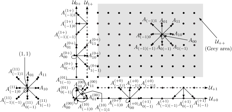
Figure 1: Regions ${\cal U}_{ss^{\prime}}$ and transition probability matrices $A_{ij}$ and $A^{(ss^{\prime})}_{ij}$

Those assumptions on the transition probabilities are essentially the same as those introduced by Ozawa [36], while there is some minor flexibility in our assumption that $A^{(11)}_{0(-1)}$ ($A^{(11)}_{(-1)0}$) may be different from $A^{(+1)}_{0(-1)}$ ($A^{(1+)}_{(-1)0}$, respectively), which are identical in [36]. Another difference is in that we have nine families of transition matrices while Ozawa [36] expresses them by four families, $A^{(s)}_{ij}$ for $s=0,1,2$ and $A_{ij}$.

By the homogeneity and independence assumptions, we can define $Z_{n+1}$ in terms of $Z_{n}$ and independent increments as

$$({\boldsymbol{L}}_{n+1},J_{n+1})=\Big{(}{\boldsymbol{L}}_{n}+\sum_{s,s^{\prime}\in{\cal A}}{\boldsymbol{X}}^{(ss^{\prime})}_{n}(J_{n})1({\boldsymbol{L}}_{n}\in{\cal U}_{ss^{\prime}}),J_{n+1}\Big{)},$$ (3.3)

where ${\boldsymbol{X}}^{(ss^{\prime})}_{n}(k)$ is the increment at time $n$ when the random walk component on ${\cal U}_{ss^{\prime}}$ and the background state is $k$. By the modeling assumption, ${\boldsymbol{X}}^{(ss^{\prime})}_{n}(k)$ is independent of $Z_{\ell}$ for $\ell\leq n-1$ and ${\boldsymbol{L}}_{n}$ for given $s,s^{\prime}$ and $k$.

The 2d-QBD process is a natural model for a two node queueing network under various situations including a Markovian arrival process and phase-type service time distributions. Its stationary distribution is a key characteristic for performance evaluation, but hard to get. This is even the case for a two dimensional reflecting random walk, which does not have background states (e.g., see [28]). Thus, recent interest has been directed to the tail asymptotics of the stationary distribution.

3.2 Markov additive kernel and stability

Recall that the 2d-QBD process is denoted by $\{(L_{1n},L_{2n},J_{n});n=0,1,\ldots\}$. To define the 1-dimensional QBD process, for $i=1,2$, let $L^{(i)}_{n}=L_{in}$ and ${\boldsymbol{J}}^{(i)}_{n}=(L_{(3-i)n},J_{n})$, then they represent level and background state at time $n$, respectively. Thus, $\{(L^{(i)}_{n},{\boldsymbol{J}}^{(i)}_{n});n\geq 0\}$ is a one-dimensional QBD process for $i=1,2$. Denote its transition matrix by $P^{(i)}$. For example, $P^{(1)}$ is given by

$$P^{(1)}=\left(\begin{matrix}N^{(1)}_{0}&N^{(1)}_{1}&0&\ldots&\ldots&\ldots&\cr N^{(1)}_{-1}&Q^{(1)}_{0}&Q^{(1)}_{1}&0&0&\ldots\cr 0&Q^{(1)}_{-1}&Q^{(1)}_{0}&Q^{(1)}_{1}&0&\ddots\cr 0&0&Q^{(1)}_{-1}&Q^{(1)}_{0}&Q^{(1)}_{1}&\ddots\cr\vdots&\vdots&\ddots&\ddots&\ddots&\ddots\end{matrix}\right),$$

where, using $(-j)^{+}=\max(0,-j)$,

$$N^{(1)}_{j}=\left(\begin{matrix}A^{((-j)^{+}0)}_{j0}&A^{((-j)^{+}0)}_{j1}&0&0&\cdots\cr A^{((-j)^{+}1)}_{j(-1)}&A^{((-j)^{+}+)}_{j0}&A^{((-j)^{+}+)}_{j1}&0&\cdots\cr 0&A^{((-j)^{+}+)}_{j(-1)}&A^{((-j)^{+}+)}_{j0}&A^{((-j)^{+}+)}_{j1}&\ddots\cr\vdots&\vdots&\ddots&\ddots&\ddots\end{matrix}\right),$$

$$Q^{(1)}_{j}=\left(\begin{matrix}A^{(+0)}_{j0}&A^{(+0)}_{j1}&0&0&\cdots\cr A^{(+1)}_{j(-1)}&A_{j0}&A_{j1}&0&\cdots\cr 0&A_{j(-1)}&A_{j0}&A_{j1}&\ddots\cr\vdots&\vdots&\ddots&\ddots&\ddots\end{matrix}\right),\qquad j=0,1,-1.$$

We next introduce the Markov additive process by removing the boundary at level $0$ of the one dimensional QBD process generated by $P^{(1)}$, and denote its transition probability matrix by $\underline{P}^{(1)}$. That is,

$$\underline{P}^{(1)}=\left(\begin{matrix}\ddots&\ddots&\ddots&\ddots&\ddots&\ddots&\ddots\cr\ddots&Q^{(1)}_{-1}&Q^{(1)}_{0}&Q^{(1)}_{1}&0&0&\cdots\cr\cdots&0&Q^{(1)}_{-1}&Q^{(1)}_{0}&Q^{(1)}_{1}&0&\ddots\cr\cdots&0&0&Q^{(1)}_{-1}&Q^{(1)}_{0}&Q^{(1)}_{1}&\ddots\cr\ddots&\ddots&\ddots&\ddots&\ddots&\ddots&\ddots\end{matrix}\right).$$

$\underline{P}^{(2)}$ and $Q^{(2)}_{i}$’s are similarly defined exchanging the coordinates. For $i=1,2$, let

$$Q^{(i)}=Q^{(i)}_{-1}+Q^{(i)}_{0}+Q^{(i)}_{1},$$

then $Q^{(i)}$ is stochastic. Let ${\boldsymbol{\nu}}^{(i)}\equiv\{{\boldsymbol{\nu}}^{(i)}_{\ell};\ell=0,1,\ldots\}$ be the left invariant positive vector of $Q^{(i)}$ when it exists, where ${\boldsymbol{\nu}}^{(i)}_{\ell}$ is $m_{0}$ and $m$-dimensional vectors for $\ell=0$ and $\ell\geq 1$, respectively. Define

$$Q^{(i)}_{*}(\theta)=e^{-\theta}Q^{(i)}_{-1}+Q^{(i)}_{0}+e^{\theta}Q^{(i)}_{1},\qquad i=1,2.$$

In order to discuss the stability of the 2d-QBD process, we define the mean drifts $\mu^{(i)}_{i}$ for each $i=1,2$ as

$$\mu^{(i)}_{i}={\boldsymbol{\nu}}^{(i)}\frac{d}{d\theta}Q^{(i)}_{*}(\theta)|_{\theta=0}{\boldsymbol{1}},$$

as long as $Q^{(i)}$ is positive recurrent, where the derivative of a matrix function is taken entry-wise. Let $A=\sum_{j,k\in\mathbb{H}}A_{jk}$. Since $A$ is stochastic and finite dimensional, it has a stationary distribution. We denote it by the row vector ${\boldsymbol{\nu}}^{(+)}$. Define the mean drifts $\mu_{1}$ and $\mu_{2}$ as

$$\mu_{1}={\boldsymbol{\nu}}^{(+)}\sum_{k\in\mathbb{H}}(-A_{(-1)k}+A_{1k}){\boldsymbol{1}},\qquad\mu_{2}={\boldsymbol{\nu}}^{(+)}\sum_{j\in\mathbb{H}}(-A_{j(-1)}+A_{j1}){\boldsymbol{1}}.$$

Note that, if $\mu_{i}<0$, then $Q^{(i)}$ is positive recurrent because $\mu_{i}$ is the mean drift at off-boundary states of the QBD process generated by $Q^{(i)}$. We refer to the recent result due to Ozawa [36].

Lemma 3.1 (Theorem 5.1 and Remark 5.1 of Ozawa [35])

The 2d-QBD process $\{Z_{n}\}$ is positive recurrent if either one of the following three conditions holds.

• If $\mu_{1}<0$ and $\mu_{2}<0$, then $\mu^{(1)}_{1}<0$ and $\mu^{(2)}_{2}<0$.

• If $\mu_{1}\geq 0$ and $\mu_{2}<0$, then $\mu^{(1)}_{1}<0$.

• If $\mu_{1}<0$ and $\mu_{2}\geq 0$, then $\mu^{(2)}_{2}<0$.

On the other hand, if $\mu_{1}>0$ and $\mu_{2}>0$, then the 2d-QBD process is transient. Hence, if $(\mu_{1},\mu_{2})\neq{\boldsymbol{0}}$, then $\{Z_{n}\}$ is positive recurrent if and only if one of the conditions (i)–(iii) holds.

Remark 3.1

The stability conditions of this lemma are exactly the same as those of the two dimensional reflecting random walk on the lattice quarter plane of [10], which is called a double QBD process in [27] (see also [19]). This is not surprising because the stability is generally determined by the mean drifts of so called induced Markov chains, which are generated by removing one of the boundary faces. However, its proof requires careful mathematical arguments, which have been done by Ozawa [36].

Throughout the paper, we assume that the 2d-QBD process has a stationary distribution, which is denoted by the row vector ${\boldsymbol{\pi}}\equiv\{\pi({\boldsymbol{z}},k);({\boldsymbol{z}},k)\in{\cal S}\}$. Lemma 3.1 can be used to verify this stability assumption. However, it is not so useful in application because the signs of $\mu^{(1)}_{1}$ and $\mu^{(2)}_{2}$ are hard to get. Thus, we will not use Lemma 3.1 in our arguments. We will return to this issue later.

3.3 Tail asymptotics for the stationary distribution

Ozawa [36] studies the tail asymptotics of the stationary distribution of the 2d-QBD process in coordinate directions, assuming stability and some additional assumptions. His arguments are based on the sufficiency part of Theorem 2.1. As discussed at the end of Section 2.3, this is intractable for applications. So far, we will consider the problem in a different way. In the first part of this section, we derive upper and lower bounds for the tail decay rates using relatively easy conditions. We then assume an extra condition similar to Assumption 2.1, and derive the tail decay rate of the marginal stationary distribution in an arbitrary direction.

To describe the modeling primitives, we will use the following matrix moment generating functions.

$$A_{**}({\boldsymbol{\theta}})=\sum_{j,k\in\mathbb{H}}e^{-(j\theta_{1}+k\theta_{2})}A_{jk},$$

$$A_{*k}(\theta_{1})=e^{-\theta_{1}}A_{(-1)k}+A_{0k}+e^{\theta_{1}}A_{1k},\quad A_{+k}(\theta_{1})=A_{0k}+e^{\theta_{1}}A_{1k},\quad k\in\mathbb{H},$$

$$A^{(+1)}_{*(-1)}(\theta_{1})=e^{-\theta_{1}}A^{(+1)}_{(-1)(-1)}+A^{(+1)}_{0(-1)}+e^{\theta_{1}}A^{(+1)}_{1(-1)},\quad A^{(+1)}_{+k}(\theta_{1})=A_{+k}(\theta_{1}),\quad k\in\mathbb{H}_{+},$$

$$A^{(+0)}_{*k}(\theta_{1})=e^{-\theta_{1}}A^{(+0)}_{(-1)k}+A^{(+0)}_{0k}+e^{\theta_{1}}A^{(+0)}_{1k},\quad A^{(+0)}_{+k}(\theta_{1})=A^{(+0)}_{0k}+e^{\theta_{1}}A^{(+0)}_{1k},\quad k\in\mathbb{H}_{+}.$$

Similarly, $A_{j*}(\theta_{2}),A_{j+}(\theta_{2}),A^{(1+)}_{(-1)*}(\theta_{2}),A^{(1+)}_{j+}(\theta_{2}),A^{(0+)}_{j*}(\theta_{2}),A^{(0+)}_{j+}(\theta_{2})$ are defined. Thus, we have many matrix moment generating functions, but they are generated by the simple rule that subscripts $*$ and $+$ indicate taking the sums for indices in $\mathbb{H}\equiv\{0,\pm 1\}$ and $\{0,1\}$, respectively.

Similar to $C_{0}$ of (2.16), we define the $m\times m$ matrix generating functions:

$$C^{(1)}_{**}({\boldsymbol{\theta}})=A_{*+}({\boldsymbol{\theta}})+A^{(+1)}_{*(-1)}(\theta_{1})(I-A^{(+0)}_{*0}(\theta_{1}))^{-1}A^{(+0)}_{*1}(\theta_{1}),$$ (3.4)

$$C^{(2)}_{**}({\boldsymbol{\theta}})=A_{+*}({\boldsymbol{\theta}})+A^{(1+)}_{(-1)*}(\theta_{2})(I-A^{(0+)}_{0*}(\theta_{2}))^{-1}A^{(0+)}_{1*}(\theta_{2}),$$ (3.5)

where, for $i=1,2$, $c_{p}(A^{(i)}_{*0}(\theta_{i}))>1$ is assumed as long as $C^{(i)}_{**}({\boldsymbol{\theta}})$ is used.

Similar to $\Gamma^{(1d)}_{0+}$ and $\theta^{(A,C)}_{\max}$ of (2.28), let, for $i=1,2$,

$$\Gamma^{(2d)}_{i+}=\{{\boldsymbol{\theta}}\in\mathbb{R}^{2};\exists{\boldsymbol{h}}>{\boldsymbol{0}},A_{**}({\boldsymbol{\theta}}){\boldsymbol{h}}\leq{\boldsymbol{h}},C^{(i)}_{**}({\boldsymbol{\theta}}){\boldsymbol{h}}\leq{\boldsymbol{h}}\}.$$

We further need the following notation.

$$\Gamma^{(2d)}_{+}=\{{\boldsymbol{\theta}}\in\mathbb{R}^{2};\exists{\boldsymbol{h}}>{\boldsymbol{0}},A_{**}({\boldsymbol{\theta}}){\boldsymbol{h}}\leq{\boldsymbol{h}}\},\quad\Gamma^{(2d)}_{\max}=\{{\boldsymbol{\theta}}\in\mathbb{R}^{2};\exists{\boldsymbol{\theta}}^{\prime}>{\boldsymbol{\theta}},{\boldsymbol{\theta}}^{\prime}\in\Gamma^{(2d)}_{+}\}.$$

Recall that the Perron-Frobenius eigenvalue of $A_{**}({\boldsymbol{\theta}})$ is denoted by $\gamma^{(A_{**})}({\boldsymbol{\theta}})$, which is finite because $A_{**}({\boldsymbol{\theta}})$ is a finite dimensional matrix. Obviously, we have

$$\Gamma^{(2d)}_{+}=\{{\boldsymbol{\theta}}\in\mathbb{R}^{2};\gamma^{(A_{**})}({\boldsymbol{\theta}})\leq 1\}.$$ (3.6)

We now define key points for $i=1,2$.

$${\boldsymbol{\theta}}^{(i,{\Gamma})}=\arg_{{\boldsymbol{\theta}}\in\mathbb{R}^{2}}\sup\{\theta_{i}\geq 0;{\boldsymbol{\theta}}\in\Gamma^{(2d)}_{i+}\},\quad{\boldsymbol{\theta}}^{(i,\max)}=\arg_{{\boldsymbol{\theta}}\in\mathbb{R}^{2}}\sup\{\theta_{i};{\boldsymbol{\theta}}\in\Gamma^{(2d)}_{+}\}.$$

Using these points, we define the vector ${\boldsymbol{\tau}}$ by

$$\tau_{1}=\sup\{\theta_{1}\in\mathbb{R};{\boldsymbol{\theta}}\in\Gamma^{(2d)}_{1+};\theta_{2}<\theta^{(2,{\Gamma})}_{2}\},\quad\tau_{2}=\sup\{\theta_{2}\in\mathbb{R};{\boldsymbol{\theta}}\in\Gamma^{(2d)}_{2+};\theta_{1}<\theta^{(1,{\Gamma})}_{1}\}.$$ (3.7)

Note that $\tau_{i}$ is finite because $\Gamma^{(2d)}_{i+}$ is a bounded set. It is notable that, in the definitions (3.7), the condition that $A_{**}({\boldsymbol{\theta}}){\boldsymbol{h}}\leq{\boldsymbol{h}}$ can be replaced by $A_{**}({\boldsymbol{\theta}}){\boldsymbol{h}}={\boldsymbol{h}}$ or, equivalently, $\gamma^{A_{**}}({\boldsymbol{\theta}})=1$.

For $i=1,2$, define the function $\overline{\xi}^{(i)}(\theta_{3-i})$ for ${\boldsymbol{\theta}}=(\theta_{1},\theta_{2})$ as

$$\overline{\xi}^{(i)}(\theta_{3-i})=\sup\{\theta_{i}\in\mathbb{R};{\boldsymbol{\theta}}\in\Gamma^{(2d)}_{i+}\}\quad\mbox{for}\quad\theta_{3-i}\in[0,\theta^{(i,{\Gamma})}_{i}].$$

Obviously, $\overline{\xi}^{(i)}(x)$ is a convex function because $\Gamma^{(2d)}_{i+}$ is a bounded set.

As in [18, 19], it is convenient to introduce the following classifications for ${\boldsymbol{\tau}}\equiv(\tau_{1},\tau_{2})$.

• $\theta^{(1,{\Gamma})}_{2}<\theta^{(2,{\Gamma})}_{2}$ and $\theta^{(2,{\Gamma})}_{1}<\theta^{(1,{\Gamma})}_{1}$, for which ${\boldsymbol{\tau}}=(\theta^{(1,{\Gamma})}_{1},\theta^{(2,{\Gamma})}_{2})$.

• $\theta^{(1,{\Gamma})}_{2}\geq\theta^{(2,{\Gamma})}_{2}$ and $\theta^{(2,{\Gamma})}_{1}<\theta^{(1,{\Gamma})}_{1}$, for which ${\boldsymbol{\tau}}=(\overline{\xi}^{(1)}(\theta^{(2,{\Gamma})}_{2}),\theta^{(2,{\Gamma})}_{2})$.

• $\theta^{(1,{\Gamma})}_{2}<\theta^{(2,{\Gamma})}_{2}$ and $\theta^{(2,{\Gamma})}_{1}\geq\theta^{(1,{\Gamma})}_{1}$, for which ${\boldsymbol{\tau}}=(\theta^{(1,{\Gamma})}_{1},\overline{\xi}^{(2)}(\theta^{(1,{\Gamma})}_{1}))$.

Since it is impossible that $\theta^{(1,{\Gamma})}_{2}\geq\theta^{(2,{\Gamma})}_{2}$ and $\theta^{(2,{\Gamma})}_{1}\geq\theta^{(1,{\Gamma})}_{1}$, these three categories completely cover the all cases (e.g., see Section 4 of [27]). These categories are crucial in our arguments as we shall see Theorem 3.2 below.

We first derive upper bounds. Let $\varphi$ be the moment generating function of ${\boldsymbol{L}}$. Namely, $\varphi({\boldsymbol{\theta}})=\mathbb{E}(e^{\langle{\boldsymbol{L}},{\boldsymbol{\theta}}\rangle})$. Define its convergence domain as

$${\cal D}=\{{\boldsymbol{\theta}}\in\mathbb{R}^{2};\exists{\boldsymbol{\theta}}^{\prime}>{\boldsymbol{\theta}},\varphi({\boldsymbol{\theta}}^{\prime})<\infty\}.$$

We prove the following lemma in Appendix D.2.

Lemma 3.2

Under the stability assumption,

$$\Gamma^{(2d)}_{{\boldsymbol{\tau}}}\equiv\{{\boldsymbol{\theta}}\in\Gamma^{(2d)}_{\max};{\boldsymbol{\theta}}<{\boldsymbol{\tau}}\}\subset{\cal D}.$$ (3.8)

Using this lemma, the following upper bound is obtained.

Theorem 3.1

Under the stability condition, we have, for each non-zero vector ${\boldsymbol{c}}\geq{\boldsymbol{0}}$,

$$\lim_{x\to\infty}\frac{1}{x}\log\mathbb{P}(\langle{\boldsymbol{L}},{\boldsymbol{c}}\rangle>x)\leq-\sup\{u\geq 0;u{\boldsymbol{c}}\in\Gamma^{(2d)}_{{\boldsymbol{\tau}}}\}.$$ (3.9)

This theorem is proved in Appendix D.3. We next derive lower bounds. We first consider lower bounds concerning the random walk component in an arbitrary direction. For this, we consider the two dimensional random walk modulated by $\{A_{jk};j,k\in\mathbb{H}\}$, which is denoted by $\{({\boldsymbol{Y}}_{n},J_{n});n\geq 1\}$. Similar to Lemma 7 of [19], we have the following fact, which is proved in Appendix E.

Lemma 3.3

For each non-zero vector ${\boldsymbol{c}}\geq{\boldsymbol{0}}$,

$$\liminf_{x\to\infty}\frac{1}{x}\log\mathbb{P}({\boldsymbol{L}}>x{\boldsymbol{c}})\geq-\sup\{\langle{\boldsymbol{\theta}},{\boldsymbol{c}}\rangle;{\boldsymbol{\theta}}\in\Gamma^{(2d)}_{+}\},$$ (3.10)

and therefore $\varphi({\boldsymbol{\theta}})$ is infinite for ${\boldsymbol{\theta}}\not\in\overline{\Gamma}^{(2d)}_{\max}$, where $\overline{\Gamma}^{(2d)}_{\max}$ is the closure of $\Gamma^{(2d)}_{\max}$.

Note that the upper bound in (3.9) is generally larger than the lower bound in (3.10). To get tighter lower bounds, we use the one dimensional QBD formulation. For this, we require assumptions similar to Assumption 2.1.

Assumption 3.1

For each ${\boldsymbol{\theta}}\in\mathbb{R}^{2}$ satisfying that $\gamma^{(A_{**})}({\boldsymbol{\theta}})=1$, for each $i=1,2$, there is an $m_{0}$-dimensional positive vector ${\boldsymbol{h}}^{(0i)}({\boldsymbol{\theta}})$ and functions $c^{(i)}_{0}({\boldsymbol{\theta}})$ and $c^{(i)}_{1}({\boldsymbol{\theta}})$ such that either one of $c^{(i)}_{1}({\boldsymbol{\theta}})$ or $c^{(i)}_{2}({\boldsymbol{\theta}})$ equals one, and

$$A^{(i)}_{*(i0)}(\theta_{i}){\boldsymbol{h}}^{(0i)}({\boldsymbol{\theta}})+e^{\theta_{2}}A^{(i)}_{*(i1)}(\theta_{i}){\boldsymbol{h}}^{(A_{**})}({\boldsymbol{\theta}})=c^{(i)}_{0}({\boldsymbol{\theta}}){\boldsymbol{h}}^{(0i)}({\boldsymbol{\theta}}),$$ (3.11)

$$e^{-\theta_{2}}A^{(i)}_{*(i(-1))}(\theta_{i}){\boldsymbol{h}}^{(0i)}({\boldsymbol{\theta}})+A_{*(i0)}(\theta_{i}){\boldsymbol{h}}^{(A_{**})}({\boldsymbol{\theta}})+e^{\theta_{2}}A_{*(i1)}(\theta_{i}){\boldsymbol{h}}^{(A_{**})}({\boldsymbol{\theta}})$$

$$\hskip 215.2771pt=c^{(i)}_{1}({\boldsymbol{\theta}}){\boldsymbol{h}}^{(A_{**})}({\boldsymbol{\theta}}),$$ (3.12)

where $*(ik)=*k$ for $i=1$ and $*(ik)=k*$ for $i=2$. We recall that ${\boldsymbol{h}}^{(A_{**})}({\boldsymbol{\theta}})$ is the Perron-Frobenius eigenvector of $A_{**}({\boldsymbol{\theta}})$.

Theorem 3.2

Assume that the 2d-QBD process has a stationary distribution and Assumption 3.1. Then, we have the following facts for each $i=1,2$. For each $\ell\geq 0$ and either $k\in{\cal V}_{1}$ for $\ell=0$ or $k\in{\cal V}_{+}$ for $\ell\geq 1$,

$$\lim_{n\to\infty}\frac{1}{n}\log\mathbb{P}(L_{i}>n,L_{3-i}=\ell,J=k)=-\tau_{i}.$$ (3.13)

In particular, for Category I satisfying $\tau_{i}<\theta^{(i,\max)}_{i}$, there is a positive constant $c^{(i)}_{\ell k}$ such that

$$\lim_{n\to\infty}e^{\tau_{i}n}\mathbb{P}(L_{i}>n,L_{3-i}=\ell,J=k)=c^{(i)}_{\ell k}.$$ (3.14)

Otherwise, for Category II-i satisfying $\tau_{i}<\theta^{(i,{\Gamma})}_{i}$, there are positive constants $\underline{d}^{(i)}_{\ell k}$ and $\overline{d}^{(i)}_{\ell k}$ such that

$$\liminf_{n\to\infty}e^{\tau_{i}n}\mathbb{P}(L_{i}>n,L_{3-i}=\ell,J=k)\geq\underline{d}^{(i)}_{\ell k},$$ (3.15)

$$\limsup_{n\to\infty}e^{\tau_{i}n}\mathbb{P}(L_{i}>n,L_{3-i}=\ell,J=k)\leq\overline{d}^{(i)}_{\ell k}.$$ (3.16)

This theorem will be proved in Appendix F. Similar results without Assumption 3.1 are obtained as Theorem 4.1 in [36]. However, the method assumes other assumptions such as Assumption 3.1 of [36]. Furthermore, it requires a large amount of numerical work to compute $\tau_{i}$.

Combining Theorems 3.1 and 3.2 and Lemma 3.3, we have the following tail asymptotics.

Theorem 3.3

Under the assumptions of Theorem 3.2, we have

$${\cal D}=\Gamma^{(2d)}_{{\boldsymbol{\tau}}}\equiv\{{\boldsymbol{\theta}}\in\Gamma^{(2d)}_{\max};{\boldsymbol{\theta}}<{\boldsymbol{\tau}}\}.$$ (3.17)

and, for each non-zero vector ${\boldsymbol{c}}\geq{\boldsymbol{0}}$,

$$\lim_{x\to\infty}\frac{1}{x}\log\mathbb{P}(\langle{\boldsymbol{L}},{\boldsymbol{c}}\rangle>x)=-\sup\{u\geq 0;u{\boldsymbol{c}}\in{\cal D}\}.$$ (3.18)

Proof. By Theorem 3.1, we already have the upper bound of the tail probability for (3.18). To consider the lower bound, let

$$u_{{\boldsymbol{c}}}=\sup\{u\geq 0;u{\boldsymbol{c}}\in{\cal D}\},\qquad{\boldsymbol{\theta}}({\boldsymbol{c}})=u_{{\boldsymbol{c}}}{\boldsymbol{c}}.$$

Note that ${\boldsymbol{\theta}}({\boldsymbol{c}})\leq{\boldsymbol{\tau}}$ by Theorem 3.1. We first assume that ${\boldsymbol{\theta}}_{{\boldsymbol{c}}}<{\boldsymbol{\tau}}$. Then, by Theorem 3.1, ${\boldsymbol{\theta}}({\boldsymbol{c}})\in\partial\Gamma^{(2d)}_{+}$, and therefore Lemma 3.3 leads to

$$\liminf_{x\to\infty}\frac{1}{x}\log\mathbb{P}(\langle{\boldsymbol{L}},{\boldsymbol{c}}\rangle>x,J=k)\geq-u_{{\boldsymbol{c}}}=-\sup\{u\geq 0;u{\boldsymbol{c}}\in{\cal D}\}.$$ (3.19)

Assume ${\boldsymbol{\theta}}_{{\boldsymbol{c}}}={\boldsymbol{\tau}}$. In this case, by Theorem 3.1, we have that $[{\boldsymbol{\theta}}({\boldsymbol{c}})]_{1}=\tau_{1}$ or $[{\boldsymbol{\theta}}({\boldsymbol{c}})]_{2}=\tau_{2}$, equivalently, $c_{1}u_{{\boldsymbol{c}}}=\tau_{1}$ or $c_{2}u_{{\boldsymbol{c}}}=\tau_{2}$. Since these two cases are symmetric, we only consider the case for $c_{1}u_{{\boldsymbol{c}}}=\tau_{1}$. By Theorem 3.2, we have, for each fixed $\ell$ and $k$,

$$\liminf_{n\to\infty}\frac{1}{n}\log\mathbb{P}(c_{1}L_{1}>n,L_{2}=\ell,J=k)\geq-\frac{\tau_{1}}{c_{1}}=-u_{{\boldsymbol{c}}}.$$

Since $c_{1}L_{1}+c_{2}L_{2}>n$ for $L_{2}=\ell$ implies that $c_{1}L_{1}>n-c_{2}\ell$, this yields

$$\liminf_{n\to\infty}\frac{1}{n}\log\mathbb{P}(\langle{\boldsymbol{L}},{\boldsymbol{c}}\rangle>x,J=k)\geq-u_{{\boldsymbol{c}}}=-\sup\{u\geq 0;u{\boldsymbol{c}}\in{\cal D}\}.$$

Thus, the limit supremum and the limit infimum are identical, and we get (3.18).

4 Two node generalized Jackson network

In this section, we consider a continuous time Markov chain $\{({\boldsymbol{L}}(t),J(t))\}$ whose embedded transitions under uniformization constitute a discrete-time 2d-QBD process. We refer it as a continuous-time 2d-QBD process. This process is convenient in queueing applications because they are often of continuous time. Since the stationary distribution is unchanged under uniformization, its tail asymptotics are also unchanged. Thus, it is routine to convert the asymptotic results obtained for the discrete-time 2d-QBD process to those for $\{({\boldsymbol{L}}(t),J(t))\}$. We summarize them for convenience of application.

4.1 Continuous time formulation of a 2d-QBD process

As discussed above, we define a continuous time 2d-QBD process $\{({\boldsymbol{L}}(t),J(t))\}$ by changing $P^{(1)}$ (or $P^{(2)}$) to a transition rate matrix. Denote it by $\tilde{P}^{(1)}$ (or $\tilde{P}^{(2)}$). That is, $\tilde{P}^{(i)}$ has the same block structure as that of $P^{(i)}$ while $\tilde{P}^{(i)}{\boldsymbol{1}}={\boldsymbol{0}}$ and all its diagonal entries are not positive. In what follows, continuous time characteristics are indicated by tilde except for those concerning the stationary distribution because the stationary distribution is unchanged. Among them, it is notable that $I-A^{(i)}_{00}$ and $I-A_{00}$ are replaced by $-\tilde{A}^{(i)}_{00}$ and $-\tilde{A}_{00}$, respectively, while $A^{(i)}_{ij}$ and $A_{ij}$ are replaced by $\tilde{A}^{(i)}_{ij}$ and $\tilde{A}_{ij}$ for $(i,j)\neq(0,0)$. Similarly, $A^{(i)}_{jk}$, $A_{**}({\boldsymbol{\theta}})$ and $C^{(i)}_{**}({\boldsymbol{\theta}})$ are defined. For example, $I-A^{(1)}_{*0}(\theta_{1})$ is replaced by $-\tilde{A}^{(1)}_{*0}(\theta_{1})$, and therefore

$$\tilde{C}^{(1)}_{**}({\boldsymbol{\theta}})=\tilde{A}_{*+}({\boldsymbol{\theta}})+\tilde{A}^{(1)}_{*(-1)}(\theta_{1})(-\tilde{A}^{(1)}_{*0}(\theta_{1}))^{-1}\tilde{A}^{(1)}_{*1}(\theta_{1}),$$

as long as $(-\tilde{A}^{(1)}_{*0}(\theta_{1}))^{-1}$ exists and is nonnegative. $\tilde{C}^{(2)}_{**}({\boldsymbol{\theta}})$ is similarly defined.

Suppose that we start with the continuous time 2d-QBD process with primitive data $\tilde{A}^{(i)}_{jk}$. These data must satisfy

$$\tilde{A}_{**}({\boldsymbol{0}}){\boldsymbol{1}}={\boldsymbol{0}},\qquad\tilde{C}^{(i)}_{**}({\boldsymbol{0}}){\boldsymbol{1}}={\boldsymbol{0}},\quad i=1,2,$$

because of the continuous time settings. Since the condition for the existence of a superharmonic vector ${\boldsymbol{h}}$ for $A_{**}({\boldsymbol{\theta}})$ is changed to $\tilde{A}_{**}({\boldsymbol{\theta}}){\boldsymbol{h}}\leq{\boldsymbol{0}}$, we define the following sets.

$$\tilde{\Gamma}^{(2d)}_{+}=\{{\boldsymbol{\theta}}\in\mathbb{R}^{2};\exists{\boldsymbol{h}}>{\boldsymbol{0}},\tilde{A}_{**}({\boldsymbol{\theta}}){\boldsymbol{h}}\leq{\boldsymbol{0}}\},$$ (4.1)

$$\tilde{\Gamma}^{(2d)}_{\max}=\{{\boldsymbol{\theta}}\in\mathbb{R}^{2};\exists{\boldsymbol{\theta}}^{\prime}>{\boldsymbol{\theta}},{\boldsymbol{\theta}}^{\prime}\in\tilde{\Gamma}^{(2d)}_{1}(\tilde{A}_{**})\},$$ (4.2)

$$\tilde{\Gamma}^{(2d)}_{i+}=\{{\boldsymbol{\theta}}\in\mathbb{R}^{2};\exists{\boldsymbol{h}}>{\boldsymbol{0}},\tilde{A}_{**}({\boldsymbol{\theta}}){\boldsymbol{h}}\leq{\boldsymbol{0}},\tilde{C}^{(i)}_{**}({\boldsymbol{\theta}}){\boldsymbol{h}}\leq{\boldsymbol{0}}\},\quad s=1,2.$$ (4.3)

The following auxiliary notation will be convenient.

$$\tilde{\Gamma}^{(2e)}_{i+}=\{{\boldsymbol{\theta}}\in\mathbb{R}^{2};\exists{\boldsymbol{h}}>{\boldsymbol{0}},\tilde{A}_{**}({\boldsymbol{\theta}}){\boldsymbol{h}}={\boldsymbol{0}},\tilde{C}^{(i)}_{**}({\boldsymbol{\theta}}){\boldsymbol{h}}\leq{\boldsymbol{0}}\},\quad i=1,2.$$ (4.4)

Using these notation, we define

$$\tilde{{\boldsymbol{\theta}}}^{(i,{\Gamma})}=\arg_{{\boldsymbol{\theta}}\in\mathbb{R}^{2}}\sup\{\theta_{i}\geq 0;{\boldsymbol{\theta}}\in\tilde{\Gamma}^{(2d)}_{i+}\},\quad\tilde{{\boldsymbol{\theta}}}^{(i,\max)}=\arg_{{\boldsymbol{\theta}}\in\mathbb{R}^{2}}\sup\{\theta_{i};{\boldsymbol{\theta}}\in\tilde{\Gamma}^{(2d)}_{+}\}.$$

and define the vector $\tilde{{\boldsymbol{\tau}}}$ by

$$\tilde{\tau}_{1}=\sup\{\theta_{1}\in\mathbb{R};{\boldsymbol{\theta}}\in\tilde{\Gamma}^{(2d)}_{1+};\theta_{2}<\tilde{\theta}^{(2,{\Gamma})}_{2}\},\quad\tilde{\tau}_{2}=\sup\{\theta_{2}\in\mathbb{R};{\boldsymbol{\theta}}\in\tilde{\Gamma}^{(2d)}_{2+};\theta_{1}<\tilde{\theta}^{(1,{\Gamma})}_{1}\}.$$ (4.5)

Remark 4.1

In the definition (4.5), we can replace $\tilde{\Gamma}^{(2d)}_{i+}$ by $\tilde{\Gamma}^{(2e)}_{i+}$ because $\tilde{\Gamma}^{(2d)}_{+}$ and $\{{\boldsymbol{\theta}}\in\mathbb{R}^{2};\tilde{C}^{(i)}_{**}({\boldsymbol{\theta}}){\boldsymbol{h}}\leq{\boldsymbol{0}}\}$ are closed convex sets.

We also need

$$\tilde{\Gamma}_{\tilde{{\boldsymbol{\tau}}}}=\{{\boldsymbol{\theta}}\in\tilde{\Gamma}^{(2d)}_{\max}(\tilde{A});{\boldsymbol{\theta}}<\tilde{{\boldsymbol{\tau}}}\}.$$ (4.6)

Let $\tilde{\gamma}^{\tilde{A}_{**}}({\boldsymbol{\theta}})$ be the Perron-Frobenius eigenvalue of $\tilde{A}_{**}({\boldsymbol{\theta}})$. A continuous time version of Assumption 3.1 is given by

Assumption 4.1

For each ${\boldsymbol{\theta}}\in\mathbb{R}^{2}$ satisfying that $\gamma^{(\tilde{A}_{**})}({\boldsymbol{\theta}})=1$, for each $i=1,2$, there is an $m_{0}$-dimensional positive vector $\tilde{{\boldsymbol{h}}}^{(i0)}({\boldsymbol{\theta}})$ and functions $\tilde{c}^{(i)}_{0}({\boldsymbol{\theta}})$ and $\tilde{c}^{(i)}_{1}({\boldsymbol{\theta}})$ such that one of $\tilde{c}^{(i)}_{0}({\boldsymbol{\theta}})$ or $\tilde{c}^{(i)}_{1}({\boldsymbol{\theta}})$ vanishes, and, for $i=1$,

$$\tilde{A}^{(+0)}_{*0}(\theta_{1})\tilde{{\boldsymbol{h}}}^{(10)}({\boldsymbol{\theta}})+e^{\theta_{2}}\tilde{A}^{(+0)}_{*1}(\theta_{1})\tilde{{\boldsymbol{h}}}^{(A_{**})}({\boldsymbol{\theta}})=\tilde{c}^{(1)}_{0}({\boldsymbol{\theta}})\tilde{{\boldsymbol{h}}}^{(10)}({\boldsymbol{\theta}}),$$ (4.7)

$$e^{-\theta_{2}}\tilde{A}^{(+1)}_{*(-1)}(\theta_{1})\tilde{{\boldsymbol{h}}}^{(10)}({\boldsymbol{\theta}})+\tilde{A}_{*+}(\theta_{1})\tilde{{\boldsymbol{h}}}^{(\tilde{A}_{**})}({\boldsymbol{\theta}})=\tilde{c}^{(1)}_{1}({\boldsymbol{\theta}})\tilde{{\boldsymbol{h}}}^{(\tilde{A}_{**})}({\boldsymbol{\theta}}),\qquad$$ (4.8)

and, for $i=2$,

$$\tilde{A}^{(0+)}_{0*}(\theta_{2})\tilde{{\boldsymbol{h}}}^{(20)}({\boldsymbol{\theta}})+e^{\theta_{1}}\tilde{A}^{(0+)}_{1*}(\theta_{2})\tilde{{\boldsymbol{h}}}^{(A_{**})}({\boldsymbol{\theta}})=\tilde{c}^{(2)}_{0}({\boldsymbol{\theta}})\tilde{{\boldsymbol{h}}}^{(20)}({\boldsymbol{\theta}}),$$ (4.9)

$$e^{-\theta_{1}}\tilde{A}^{(1+)}_{(-1)*}(\theta_{2})\tilde{{\boldsymbol{h}}}^{(20)}({\boldsymbol{\theta}})+\tilde{A}_{+*}(\theta_{2})\tilde{{\boldsymbol{h}}}^{(\tilde{A}_{**})}({\boldsymbol{\theta}})=\tilde{c}^{(2)}_{1}({\boldsymbol{\theta}})\tilde{{\boldsymbol{h}}}^{(\tilde{A}_{**})}({\boldsymbol{\theta}}).\qquad$$ (4.10)

We recall that $\tilde{{\boldsymbol{h}}}^{(\tilde{A}_{**})}({\boldsymbol{\theta}})$ is the Perron-Frobenius eigenvector of $\tilde{A}_{**}({\boldsymbol{\theta}})$.

Define the domain for the stationary distribution of ${\boldsymbol{L}}$ as

$${\cal D}=\mbox{the interior of }\{{\boldsymbol{\theta}}\in\mathbb{R}^{2};\mathbb{E}(e^{\langle{\boldsymbol{\theta}},{\boldsymbol{L}}\rangle})<\infty\},$$ (4.11)

where ${\boldsymbol{L}}$ is a random vector subject to the stationary distribution of ${\boldsymbol{L}}(t)$. It is easy to see that Theorems 3.1 and 3.3 can be combined and converted into the following continuous version.

Theorem 4.1

For a continuous-time 2d-QBD process satisfying the irreducibility and stability conditions, $\tilde{\Gamma}_{\tilde{{\boldsymbol{\tau}}}}\subset{\cal D}$ and we have

$$\lim_{x\to\infty}\frac{1}{x}\log\mathbb{P}(\langle{\boldsymbol{L}},{\boldsymbol{c}}\rangle>x)\leq-\sup\{u\geq 0;u{\boldsymbol{c}}\in\tilde{\Gamma}_{\tilde{{\boldsymbol{\tau}}}}\},$$ (4.12)

and this inequality becomes equality with ${\cal D}=\tilde{\Gamma}_{\tilde{{\boldsymbol{\tau}}}}$ if Assumption 4.1 is satisfied.

4.2 Two node generalized Jackson network with MAP arrivals and PH-service time distributions

As an example of the 2d-QBD process, we consider a two node generalized Jackson network with a MAP arrival process and phase type service time distributions. Obviously, this model can be formulated as a 2d-QBD process. We are interested to see how exogenous arrival processes and service time distributions influence the decay rates. This question has been partially answered for the tail decay rates of the marginal distributions of tandem queues with stationary or renewal inputs (e.g. see [3, 14]). They basically use the technique for sample path large deviations, and no joint distributions has been studied for queue lengths at multiple nodes. For Markov modulated arrivals and more general network topologies, there is seminal work by Takahashi and his colleagues [11, 12, 15, 16]. They started with numerical examinations and finally arrived at upper bounds for the stationary tail probabilities for the present generalized Jackson network in [16]. The author [26] conjectured the tail decay rates of the stationary distribution for a $d$-node generalized Jackson network with $d\geq 2$ and renewal arrivals.

Thus, the question has not yet been satisfactorily answered particularly for a network with feedback routes. This motivates us to study the present decay rate problem. As we will see, the answer is relatively simple, and naturally generalizes the tandem queue case. However, first we have to introduce yet more notation to describe the generalized Jackson network. This network has two nodes, which are numbered as $1$ and $2$. We make the following modeling assumptions.

• A customer which completes service at node $i$ goes to node $j$ with probability $r_{ij}$ or leaves the network with probability $1-r_{ij}$ for $(i,j)=(1,2)$ or $(2,1)$, where $r_{12}+r_{21}>0$ and $r_{12}r_{21}<1$, which exclude obvious cases. This routing of customers is assumed to be independent of everything else.

• Exogenous customers arrive at node $i$ subject to the Markovian arrival process with generator ${T}_{i}+{U}_{i}$, where ${U}_{i}$ generates arrivals. Here, ${T}_{i}$ and ${U}_{i}$ are finite square matrices of the same size for each $i=1,2$.

• Node $i$ has a single server, whose service times are independently and identically distributed subject to a phase type distribution with $({\boldsymbol{\beta}}_{i},{S}_{i})$, where ${\boldsymbol{\beta}}_{i}$ is the row vector representing the initial phase distribution and ${S}_{i}$ is a transition rate matrix for internal state transitions. Here, ${S}_{i}$ is a finite square matrix, and ${\boldsymbol{\beta}}_{i}$ has the same dimension as that of ${S}_{i}$ for each $i=1,2$.

Let ${D}_{i}=(-{S}_{i}{\boldsymbol{1}}){\boldsymbol{\beta}}_{i}$, then ${S}_{i}+{D}_{i}$ is a generator for a continuous time Markov chain which generates completion of service times with rate ${D}_{i}$. Since the service time distribution at node $i$ has the phase type distribution with $({\boldsymbol{\beta}}_{i},{S}_{i})$, its moment generating function $g_{i}$ of is given by

$$g_{i}(\theta)=\langle{\boldsymbol{\beta}}_{i},(-\theta I_{i+2}-{S}_{i})^{-1}(-{S}_{i}{\boldsymbol{1}})\rangle,\qquad i=1,2,$$ (4.13)

as long as $\theta I_{i+2}+{S}_{i}$ is non-singular (e.g., see [21] in which the Laplace transform is used instead of the moment generating function). Clearly, $g_{i}(\theta)$ is a increasing function of $\theta$ from $(-\infty,\theta_{0i})$ to $(0,\infty)$, where $-\theta_{0i}$ is the Perron-Frobenius eigenvalue of $S_{i}$.

Let $L_{i}(t)$, $J_{ia}(t)$ and $J_{ib}(t)$ be the number of customers at node $i$, the background state for arrivals and the phase of service in progress, respectively, at time $t$, where $J_{ib}(t)$ is undefined if there is no customer in node $i$ at time $t$. Then, it is not hard to see that $\{({\boldsymbol{L}}(t),{\boldsymbol{J}}(t));t\geq 0\}$ is a continuous-time Markov chain and considered as a 2d-QBD process, where ${\boldsymbol{L}}(t)=(L_{1}(t),L_{2}(t))$ and ${\boldsymbol{J}}(t)=(J_{1a}(t),J_{2a}(t),J_{1b}(t),J_{2b}(t))$, where $J_{ib}(t)$ is removed from the components of ${\boldsymbol{J}}(t)$ if it is undefined.

We first note the stability condition for this 2d-QBD process. Since, for node $i$, the mean exogenous arrival rate $\lambda_{i}$ and the mean service rate $\mu_{i}$ are given by

$$\lambda_{i}=\langle{\boldsymbol{\nu}}_{i},U_{i}{\boldsymbol{1}}_{i}\rangle\qquad\mu_{i}=\langle{\boldsymbol{\beta}}_{i},(-S_{i})^{-1}{\boldsymbol{1}}_{i}\rangle,$$

where ${\boldsymbol{\nu}}_{i}$ is the stationary distribution of the Markov chain with generator $T_{i}+U_{i}$, it is well known that the stability condition is given by

$$\rho_{i}\equiv\frac{\lambda_{i}+\lambda_{3-i}r_{(3-i)i}}{(1-r_{12}r_{21})\mu_{i}}<1,\qquad i=1,2.$$ (4.14)

We assume this condition throughout in Section 4.2.

We next introduce point processes to count arriving and departing customers from each node. By $N^{(a)}_{i}(t)$, we denote the number of exogenous arriving customers at node $i$ during the time interval $[0,t]$. Then, it follows from (4b) (also the comment above (4.14)) that

$$\mathbb{E}(e^{\theta N^{(a)}_{i}(t)}1(J(t)=k)|J(0)=j)=\left[\exp(t({T}_{i}+e^{\theta}{U}_{i}))\right]_{jk}.$$

We define a time-average cumulant moment generating function $\gamma^{(ia)}$ as

$$\gamma^{(ia)}(\theta)=\lim_{t\to\infty}\frac{1}{t}\log\mathbb{E}(e^{\theta N^{(a)}_{i}(t)}),\qquad i=1,2.$$ (4.15)

It is not hard to see that $\gamma^{(ia)}(\theta)$ is the Perron-Frobenius eigenvalue of ${T}_{i}+e^{\theta}{U}_{i}$.

By $N^{(d)}_{i}(t)$, we denote the number of departing customers from node $i$ during the time interval $[0,t]$ when the server at node $i$ is always busy in this time interval. Let $\Phi_{i}(n)$ be the number of customers who are routed to node $3-i$ among $n$ customers departing from node $i$. Obviously, it follows from (4a) that $\Phi_{i}(n)$ is independent of $N^{(d)}_{i}(t)$, and has the Bernoulli distribution with parameter $(n,r_{i(3-i)})$. Then,

$$\mathbb{E}(e^{-\theta_{i}N^{(d)}_{i}(t)+\theta_{3-i}\Phi_{i}(N^{(d)}_{i}(t))}1(J(t)=k)|J(0)=j)$$

$$=\left[\exp(t({S}_{i}+e^{-\theta_{i}}(r_{i0}+e^{\theta_{3-i}}r_{i(3-i)}){D}_{i})\right]_{jk},$$

where $r_{i0}=1-r_{i(3-i)}$. Similar to $\gamma^{(ia)}$, we define a time-average cumulant moment generating function $\gamma^{(id)}$ by

$$\gamma^{(id)}({\boldsymbol{\theta}})=\lim_{t\to\infty}\frac{1}{t}\log\mathbb{E}(e^{-\theta_{i}N^{(d)}_{i}(t)+\theta_{3-i}\Phi_{i}(N^{(d)}_{i}(t))}),\qquad{\boldsymbol{\theta}}=(\theta_{1},\theta_{2}),\;i=1,2.$$

One can see that $\gamma^{(id)}({\boldsymbol{\theta}})$ is the Perron-Frobenius eigenvalue of ${S}_{i}+e^{-\theta_{i}}(r_{i0}+e^{\theta_{3-i}}r_{i(3-i)}){D}_{i}$.

One may expect that the decay rates for the generalized Jackson network are completely determined by the cumulants $\gamma^{(1a)},\gamma^{(2a)},\gamma^{(1d)},\gamma^{(2d)}$ since their conjugates are known to be rate functions for the Cramér type of large deviations. We will show that this is indeed the case. Let

$$\gamma^{(+)}({\boldsymbol{\theta}})=\gamma^{(1a)}(\theta_{1})+\gamma^{(2a)}(\theta_{2})+\gamma^{(1d)}({\boldsymbol{\theta}})+\gamma^{(2d)}({\boldsymbol{\theta}}),$$

$$\gamma^{(i)}({\boldsymbol{\theta}})=\gamma^{(1a)}(\theta_{1})+\gamma^{(2a)}(\theta_{2})+\gamma^{(id)}({\boldsymbol{\theta}}),\qquad i=1,2.$$

We then have the following result.

Theorem 4.2

For the generalized Jackson network satisfying conditions (4a) (4b) and (4c), if the stability condition (4.14) holds, then Assumption 4.1 is satisfied, and we have

$$\tilde{\Gamma}^{2d}_{+}=\{{\boldsymbol{\theta}}\in\mathbb{R}^{2};\gamma^{(+)}({\boldsymbol{\theta}})\leq 0\},$$ (4.16)

$$\tilde{\Gamma}^{2e}_{i+}=\{{\boldsymbol{\theta}}\in\mathbb{R}^{2};\gamma^{(+)}({\boldsymbol{\theta}})=0,\gamma^{(i)}({\boldsymbol{\theta}})\leq 0\},\quad i=1,2.\quad$$ (4.17)

Define $\tilde{\tau}$ and $\tilde{\Gamma}_{\tilde{\tau}}$ by (4.5) and (4.6), then the domain ${\cal D}$ for ${\boldsymbol{L}}$ is given by $\tilde{\Gamma}_{\tilde{{\boldsymbol{\tau}}}}$ and, for non-zero vector ${\boldsymbol{c}}\geq{\boldsymbol{0}}$,

$$\lim_{x\to\infty}\frac{1}{x}\log\mathbb{P}(\langle{\boldsymbol{L}},{\boldsymbol{c}}\rangle>x)=-\sup\{u\geq 0;u{\boldsymbol{c}}\in\tilde{\Gamma}_{\tilde{{\boldsymbol{\tau}}}}\},$$ (4.18)

where ${\boldsymbol{L}}$ is a random vector subject to the stationary distribution of ${\boldsymbol{L}}(t)$.

Remark 4.2

As we will show at the end of Section 4.4, the condition that $\gamma^{(i)}({\boldsymbol{\theta}})\leq 0$ in (4.17) can be replaced by $e^{-\theta_{3-i}}(r_{(3-i)0}+e^{\theta_{i}}r_{(3-i)i})\geq 1$.

Remark 4.3

For ${\boldsymbol{c}}=(1,0),(0,1)$, Katou et al. [15] obtained the right-hand side of (4.18) as an upper bound for its left-hand side (see Theorem 4.1 there). Namely, they derived the inequality (4.12), which is conjectured to be tight in [26]. Theorem 4.2 shows that those upper bounds are indeed tight. Based on the results in [15], Katou et al. [16] derived upper bounds for the decay rate of the probability $\mathbb{P}({\boldsymbol{L}}=n{\boldsymbol{c}}+{\boldsymbol{d}})$ for positive vectors ${\boldsymbol{c}},{\boldsymbol{d}}$ with integer entries as $n\to\infty$, and numerically examined their tightness. This asymptotic is different from that in (4.18), so we can not confirm its tightness by (4.18), but conjecture it to be true since similar asymptotics are known for a two dimensional semimartingale reflecting Brownian motion (see [1, 9]).

See Figure 2 to see how the domain looks like.

 

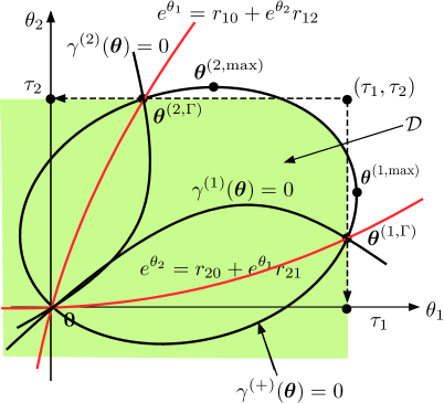
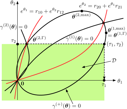
Figure 2: The domain ${\cal D}$ for the two node generalized Jackson network

4.3 Primitive data and matrix moment generation functions

In this section, we describe transition rate matrices and their moment generating functions in terms of the primitive data, $T_{i},U_{i},S_{i},{\boldsymbol{\beta}}_{i}$, of the generalized Jackson network, and prove (4.16) and (4.17). They will be used to prove Theorem 4.2 in the next subsection.

To specify those matrices for the generalized Jackson network, we will use the Kronecker product $\otimes$ and sum $\oplus$, respectively, where $\oplus$ is defined for square matrices $A$ and $B$ as

$$A\oplus B=A\otimes I_{2}+I_{1}\otimes B,$$

where $I_{1}$ and $I_{2}$ are the identity matrices with the same sizes as $A$ and $B$, respectively. From this definition, it is easy to see that. if $A$ and $B$ have right eigenvectors ${\boldsymbol{h}}_{A}$ and ${\boldsymbol{h}}_{A}$ with eigenvalues $\gamma_{A}$ and $\gamma_{B}$, respectively, then

$$(A\oplus B)({\boldsymbol{h}}_{A}\otimes{\boldsymbol{h}}_{B})=(\gamma_{A}+\gamma_{B})({\boldsymbol{h}}_{A}\otimes{\boldsymbol{h}}_{B}).$$ (4.19)

We also will use this computation.

For transitions around the origin, we let

$$\tilde{A}^{(0)}_{00}={T}_{1}\oplus{T}_{2},\quad\tilde{A}^{(0)}_{10}={U}_{1}\otimes I_{2}\otimes{\boldsymbol{\beta}}_{1},\quad\tilde{A}^{(0)}_{01}=I_{1}\otimes{U}_{2}\otimes{\boldsymbol{\beta}}_{2},$$

$$\tilde{A}^{(0)}_{(-1)0}=I_{1}\otimes I_{2}\otimes{D}_{1}{\boldsymbol{1}},\quad\tilde{A}^{(0)}_{0(-1)}=I_{1}\otimes I_{2}\otimes{D}_{2}{\boldsymbol{1}},$$

where other $\tilde{A}^{(0)}_{ij}$’s not specified above are all null matrices. This convention for null matrices is used for all transition matrices. Around ${\cal U}_{+0}\cup{\cal U}_{+1}$, that is, the 1st coordinate half axis except for the origin,

$$\tilde{A}^{(1)}_{(-1)0}=I_{1}\otimes I_{2}\otimes(r_{10}{D}_{1})\quad\tilde{A}^{(1)}_{00}={T}_{1}\oplus{T}_{2}\oplus{S}_{1},\quad\tilde{A}^{(1)}_{10}={U}_{1}\otimes I_{2}\otimes I_{3},$$

$$\tilde{A}^{(1)}_{(-1)1}=I_{1}\otimes I_{2}\otimes(r_{12}{D}_{1})\otimes{\boldsymbol{\beta}}_{2}\quad\tilde{A}^{(1)}_{01}=I_{1}\otimes{U}_{2}\otimes I_{3}\otimes{\boldsymbol{\beta}}_{2},$$

$$\tilde{A}^{(1)}_{0(-1)}=I_{1}\otimes I_{2}\otimes I_{3}\otimes(r_{20}{D}_{2}{\boldsymbol{1}}),\quad\tilde{A}^{(1)}_{1(-1)}=I_{1}\otimes I_{2}\otimes I_{3}\otimes(r_{21}{D}_{2}{\boldsymbol{1}}).$$

Similarly, around ${\cal U}_{0+}\cup{\cal U}_{1+}$, that is, the 2nd coordinate half axis except for the origin,

$$\tilde{A}^{(2)}_{0(-1)}=I_{1}\otimes I_{2}\otimes(r_{20}{D}_{2}),\quad\tilde{A}^{(2)}_{00}={T}_{1}\oplus{T}_{2}\oplus{S}_{2},\quad\tilde{A}^{(2)}_{01}=I_{1}\otimes{U}_{2}\otimes I_{4},$$

$$\tilde{A}^{(2)}_{1(-1)}=I_{1}\otimes I_{2}\otimes{\boldsymbol{\beta}}_{1}\otimes(r_{21}{D}_{2}),\quad\tilde{A}^{(2)}_{10}={U}_{1}\otimes I_{2}\otimes{\boldsymbol{\beta}}_{1}\otimes I_{4},$$

$$\tilde{A}^{(2)}_{(-1)0}=I_{1}\otimes I_{2}\otimes(r_{10}{D}_{1}{\boldsymbol{1}})\otimes I,\quad\tilde{A}^{(2)}_{(-1)1}=I_{1}\otimes I_{2}\otimes(r_{12}{D}_{1}{\boldsymbol{1}})\otimes I_{4}.$$

For transitions within ${\cal U}_{+}$, that is, the interior,

$$\tilde{A}_{00}={T}_{1}\oplus{T}_{2}\oplus{S}_{1}\oplus{S}_{2},\quad\tilde{A}_{10}={U}_{1}\otimes I_{2}\otimes I_{2}\otimes I_{3},\quad\tilde{A}_{01}=I_{1}\otimes{U}_{2}\otimes I_{3}\otimes I_{4},$$

$$\tilde{A}_{(-1)0}=I_{1}\otimes I_{2}\otimes(r_{10}{D}_{1})\otimes I_{4},\quad\tilde{A}_{(-1)1}=I_{1}\otimes I_{2}\otimes(r_{12}{D}_{1})\otimes I_{4},$$

$$\tilde{A}_{0(-1)}=I_{1}\otimes I_{2}\otimes I_{3}\otimes(r_{20}{D}_{2}),\quad\tilde{A}_{1(-1)}=I_{1}\otimes I_{2}\otimes I_{3}\otimes(r_{21}{D}_{2}).$$

Thus, we have

$$\tilde{A}_{**}({\boldsymbol{\theta}})=({T}_{1}+e^{\theta_{1}}{U}_{1})\oplus({T}_{2}+e^{\theta_{2}}{U}_{2})$$

$$\oplus({S}_{1}+(e^{-\theta_{1}}r_{10}+e^{-\theta_{1}+\theta_{2}}r_{12}){D}_{1})\oplus({S}_{2}+(e^{-\theta_{2}}r_{20}+e^{\theta_{1}-\theta_{2}}r_{21}){D}_{2}).$$

Recall that $\gamma^{(ia)}(\theta_{i})$ is the Perron-Frobenius eigenvalue of ${T}_{i}+e^{\theta_{i}}{U}_{i}$. We denote its eigenvector by ${\boldsymbol{h}}^{(ia)}(\theta_{i})$. Similarly, we denote the Perron-Frobenius eigenvalues and vectors of ${S}_{1}+(e^{-\theta_{1}}r_{10}+e^{-\theta_{1}+\theta_{2}}r_{12}){D}_{1}$ and ${S}_{2}+(e^{-\theta_{2}}r_{20}+e^{\theta_{1}-\theta_{2}}r_{21}){D}_{2}$ by $\gamma^{(1d)}({\boldsymbol{\theta}})$ and $\gamma^{(2d)}({\boldsymbol{\theta}})$, and ${\boldsymbol{h}}^{(1d)}({\boldsymbol{\theta}})$ and ${\boldsymbol{h}}^{(1d)}({\boldsymbol{\theta}})$, respectively. That is, they satisfy

$$({T}_{1}+e^{\theta_{1}}{U}_{1}){\boldsymbol{h}}^{(1a)}(\theta_{1})=\gamma^{(1a)}(\theta_{1}){\boldsymbol{h}}^{(1a)}(\theta_{1}),$$ (4.20)

$$({T}_{2}+e^{\theta_{2}}{U}_{2}){\boldsymbol{h}}^{(2a)}(\theta_{2})=\gamma^{(2a)}(\theta_{2}){\boldsymbol{h}}^{(2a)}(\theta_{2}),$$ (4.21)

$$({S}_{1}+(e^{-\theta_{1}}r_{10}+e^{-\theta_{1}+\theta_{2}}r_{12}){D}_{1}){\boldsymbol{h}}^{(1d)}({\boldsymbol{\theta}})=\gamma^{(1d)}({\boldsymbol{\theta}}){\boldsymbol{h}}^{(1d)}({\boldsymbol{\theta}}),$$ (4.22)

$$({S}_{2}+(e^{-\theta_{2}}r_{20}+e^{\theta_{1}-\theta_{2}}r_{21}){D}_{2}){\boldsymbol{h}}^{(2d)}({\boldsymbol{\theta}})=\gamma^{(2d)}({\boldsymbol{\theta}}){\boldsymbol{h}}^{(2d)}({\boldsymbol{\theta}}).$$ (4.23)

Thus, recalling $\gamma^{(+)}({\boldsymbol{\theta}})$ and letting

$${\boldsymbol{h}}^{(+)}({\boldsymbol{\theta}})={\boldsymbol{h}}^{(1a)}(\theta_{1})\otimes{\boldsymbol{h}}^{(2a)}(\theta_{2})\otimes{\boldsymbol{h}}^{(1d)}({\boldsymbol{\theta}})\otimes{\boldsymbol{h}}^{(2d)}({\boldsymbol{\theta}}),$$

we have, by repeatedly applying (4.19),

$$\tilde{A}_{**}({\boldsymbol{\theta}}){\boldsymbol{h}}^{(+)}({\boldsymbol{\theta}})=\gamma^{(+)}({\boldsymbol{\theta}}){\boldsymbol{h}}^{(+)}({\boldsymbol{\theta}}).$$

Hence, recalling the definition (4.1) of $\tilde{\Gamma}^{(2d)}$, we have (4.16).

We next note that $\gamma^{(id)}$ can also be obtained from the moment generating function $g_{i}$ of service time distribution at node $i$. For $i=1,2$, let

$$t_{i}({\boldsymbol{\theta}})=e^{-\theta_{i}}r_{i0}+e^{-\theta_{i}+\theta_{3-i}}r_{i(3-i)},$$

then it follows from (4.22) and (4.23) that

$$t_{i}({\boldsymbol{\theta}})\langle{\boldsymbol{\beta}}_{i},{\boldsymbol{h}}^{(id)}({\boldsymbol{\theta}})\rangle(-S_{i}{\boldsymbol{1}})=(\gamma^{(id)}({\boldsymbol{\theta}})I-S_{i}){\boldsymbol{h}}^{(id)}({\boldsymbol{\theta}}),$$

since $D_{i}{\boldsymbol{h}}^{(id)}({\boldsymbol{\theta}})=\langle{\boldsymbol{\beta}}_{i},{\boldsymbol{h}}^{(id)}({\boldsymbol{\theta}})\rangle(-S_{i}{\boldsymbol{1}})$. Hence, premultiplying $(\gamma^{(id)}({\boldsymbol{\theta}})I-S_{i})^{-1}$, we have

$${\boldsymbol{h}}^{(id)}({\boldsymbol{\theta}})=t_{i}({\boldsymbol{\theta}})\langle{\boldsymbol{\beta}}_{i},{\boldsymbol{h}}^{(id)}({\boldsymbol{\theta}})\rangle(\gamma^{(id)}({\boldsymbol{\theta}})I-S_{i})^{-1}(-S_{i}){\boldsymbol{1}},$$

Let us normalize ${\boldsymbol{h}}^{(id)}({\boldsymbol{\theta}})$ in such a way that

$$\langle{\boldsymbol{\beta}}_{i},{\boldsymbol{h}}^{(id)}({\boldsymbol{\theta}})\rangle=t_{i}({\boldsymbol{\theta}})^{-1},$$ (4.24)

then we have the following facts since $g_{i}$ is nondecreasing.

Lemma 4.1

For $i=1,2$, (a) under the normalization (4.24),

$${\boldsymbol{h}}^{(id)}({\boldsymbol{\theta}})=(\gamma^{(id)}({\boldsymbol{\theta}})I-S_{i})^{-1}(-S_{i}){\boldsymbol{1}},$$ (4.25)

and therefore $g_{i}(-\gamma^{(id)}({\boldsymbol{\theta}}))=t_{i}({\boldsymbol{\theta}})^{-1}$, which yields $\gamma^{(id)}({\boldsymbol{\theta}})=-g_{i}^{-1}(t_{i}({\boldsymbol{\theta}})^{-1})$,
(b) $\gamma^{(id)}({\boldsymbol{\theta}})\geq 0$ if and only if $t_{i}({\boldsymbol{\theta}})\geq 1$, which is equivalent to

$$r_{i0}+e^{\theta_{3-i}}r_{i(3-i)}\geq e^{\theta_{i}}.$$ (4.26)

(c) If $U_{i}=(-T_{i}{\boldsymbol{1}}){\boldsymbol{\alpha}}_{i}$ for probability vectors ${\boldsymbol{\alpha}}_{i}$, that is, the arrival process at node $i$ is the renewal process with interarrival distribution determined by the moment generating function:

$$f_{i}(\theta_{i})=\langle{\boldsymbol{\alpha}}_{i},(-\theta_{i}I-T_{i})^{-1}(-T_{i}{\boldsymbol{1}})\rangle,$$

then $\gamma^{(ia)}(\theta_{i})=-f_{i}^{-1}(e^{-\theta_{i}})$.

Remark 4.4

(a) and (c) are known (see, e.g., Proposition 2 of [39] and Lemma 4.1 of [12]).

4.4 Proof of Theorem 4.2

We first verify Assumption 4.1 for $i=1$ and $\tilde{c}^{(1)}_{1}({\boldsymbol{\theta}})=0$, Namely, for ${\boldsymbol{\theta}}\in\mathbb{R}^{2}$ satisfying that $\gamma^{(+)}({\boldsymbol{\theta}})=0$, that is,

$$\gamma^{(1a)}(\theta_{1})+\gamma^{(2a)}(\theta_{2})+\gamma^{(1d)}({\boldsymbol{\theta}})+\gamma^{(2d)}({\boldsymbol{\theta}})=0,$$ (4.27)

we show that there are some $\tilde{c}^{(1)}_{0}({\boldsymbol{\theta}})$ and ${\boldsymbol{h}}^{(01)}({\boldsymbol{\theta}})>{\boldsymbol{0}}$ such that

$$\tilde{A}^{(1)}_{*0}(\theta_{1}){\boldsymbol{h}}^{(01)}({\boldsymbol{\theta}})+e^{\theta_{2}}\tilde{A}^{(1)}_{*1}(\theta_{1}){\boldsymbol{h}}^{(+)}({\boldsymbol{\theta}})=\tilde{c}^{(1)}_{0}({\boldsymbol{\theta}}){\boldsymbol{h}}^{(01)}({\boldsymbol{\theta}}),$$ (4.28)

$$e^{-\theta_{2}}\tilde{A}^{(1)}_{*(-1)}(\theta_{1}){\boldsymbol{h}}^{(01)}({\boldsymbol{\theta}})+\tilde{A}_{*0}(\theta_{1}){\boldsymbol{h}}^{(+)}({\boldsymbol{\theta}})+e^{\theta_{2}}\tilde{A}_{*1}(\theta_{1}){\boldsymbol{h}}^{(+)}({\boldsymbol{\theta}})={\boldsymbol{0}},\qquad$$ (4.29)

where

$$\tilde{A}_{*+}({\boldsymbol{\theta}})=({T}_{1}+e^{\theta_{1}}{U}_{1})\oplus({T}_{2}+e^{\theta_{2}}{U}_{2})\oplus({S}_{1}+(e^{-\theta_{1}}r_{10}+e^{-\theta_{1}+\theta_{2}}r_{12}){D}_{1})\oplus{S}_{2},$$

$$\tilde{A}_{*(-1)}(\theta_{1})=I_{1}\otimes I_{2}\otimes I_{3}\otimes((r_{20}+r_{21}e^{\theta_{1}}){D}_{2}),$$

$$\tilde{A}^{(1)}_{*(-1)}(\theta_{1})=I_{1}\otimes I_{2}\otimes I_{3}\otimes((r_{20}+r_{21}e^{\theta_{1}}){D}_{2}{\boldsymbol{1}}),$$

$$\tilde{A}^{(1)}_{*0}(\theta_{1})=({T}_{1}+e^{\theta_{1}}{U}_{1})\oplus{T}_{2}\oplus({S}_{1}+r_{10}e^{-\theta_{1}}{D}_{1}),$$

$$\tilde{A}^{(1)}_{*1}(\theta_{1})=I_{1}\otimes({U}_{2}\oplus(r_{12}e^{-\theta_{1}}{D}_{1}))\otimes{\boldsymbol{\beta}}_{2}.$$

We further require the non-singularity condition:

$$\tilde{A}^{(1)}_{*0}(\theta_{1}){\boldsymbol{h}}^{(01)}({\boldsymbol{\theta}})<{\boldsymbol{0}}.$$ (4.30)

From (4.28), this holds if $\tilde{c}_{0}^{(1)}({\boldsymbol{\theta}})\leq 0$.

Since $\tilde{A}_{**}({\boldsymbol{\theta}}){\boldsymbol{h}}^{(+)}({\boldsymbol{\theta}})={\boldsymbol{0}}$ by (4.27), (4.29) is equivalent to

$$\tilde{A}^{(1)}_{*(-1)}(\theta_{1}){\boldsymbol{h}}^{(01)}({\boldsymbol{\theta}})-\tilde{A}_{*(-1)}(\theta_{1}){\boldsymbol{h}}^{(+)}({\boldsymbol{\theta}})={\boldsymbol{0}}.$$ (4.31)

Note that $\tilde{A}_{*(-1)}(\theta_{1})$ and $\tilde{A}^{(1)}_{*(-1)}(\theta_{1})$ have a similar form, so we let

$${\boldsymbol{h}}^{(1)}({\boldsymbol{\theta}})={\boldsymbol{h}}^{(1a)}(\theta_{1})\otimes{\boldsymbol{h}}^{(2a)}(\theta_{2})\otimes{\boldsymbol{h}}^{(1d)}({\boldsymbol{\theta}}),$$

and guess that, for some scalar $a({\boldsymbol{\theta}})$,

$${\boldsymbol{h}}^{(01)}({\boldsymbol{\theta}})=a({\boldsymbol{\theta}}){\boldsymbol{h}}^{(1)}({\boldsymbol{\theta}}).$$

We first verify (4.28). Since

$$\tilde{A}^{(1)}_{*0}(\theta_{1}){\boldsymbol{h}}^{(01)}({\boldsymbol{\theta}})=a({\boldsymbol{\theta}})\big{(}\gamma^{(1a)}(\theta_{1}){\boldsymbol{h}}^{(1)}({\boldsymbol{\theta}})+{\boldsymbol{h}}^{(1a)}(\theta_{1})\otimes(T_{2}{\boldsymbol{h}}^{(2a)})\otimes{\boldsymbol{h}}^{(1d)}({\boldsymbol{\theta}})$$

$$\hskip 107.63855pt+{\boldsymbol{h}}^{(1a)}(\theta_{1})\otimes{\boldsymbol{h}}^{(2a)}(\theta_{2})\otimes({S}_{1}+r_{10}e^{-\theta_{1}}{D}_{1}){\boldsymbol{h}}^{(1d)}({\boldsymbol{\theta}})\big{)},$$

$$e^{\theta_{2}}\tilde{A}^{(1)}_{*1}(\theta_{1}){\boldsymbol{h}}^{(+)}({\boldsymbol{\theta}})={\boldsymbol{h}}^{(1a)}(\theta_{1})\otimes\left(e^{\theta_{2}}U_{2}{\boldsymbol{h}}^{(2a)}(\theta_{2})\otimes{\boldsymbol{h}}^{(1d)}({\boldsymbol{\theta}})\right.$$

$$\hskip 107.63855pt+\left.{\boldsymbol{h}}^{(2a)}(\theta_{2})\otimes(r_{12}e^{-\theta_{1}+\theta_{2}}D_{1}{\boldsymbol{h}}^{(1d)}({\boldsymbol{\theta}}))\right)\langle{\boldsymbol{\beta}}_{2},{\boldsymbol{h}}^{(2d)}({\boldsymbol{\theta}})\rangle,$$

we choose $a({\boldsymbol{\theta}})=\langle{\boldsymbol{\beta}}_{2},{\boldsymbol{h}}^{(2d)}({\boldsymbol{\theta}})\rangle$, which is $t_{2}({\boldsymbol{\theta}})^{-1}$ by (4.24), then

$$\tilde{A}^{(1)}_{*0}(\theta_{1}){\boldsymbol{h}}^{(01)}({\boldsymbol{\theta}})+e^{\theta_{2}}\tilde{A}^{(1)}_{*1}(\theta_{1}){\boldsymbol{h}}^{(+)}({\boldsymbol{\theta}}) =\big{(}\gamma^{(1a)}(\theta_{1})+\gamma^{(2a)}(\theta_{2})+\gamma^{(1d)}({\boldsymbol{\theta}})\big{)}{\boldsymbol{h}}^{(01)}({\boldsymbol{\theta}}).$$

Hence, we have (4.28) with

$$\tilde{c}^{(1)}_{0}({\boldsymbol{\theta}})=\gamma^{(1a)}(\theta_{1})+\gamma^{(2a)}(\theta_{2})+\gamma^{(1d)}({\boldsymbol{\theta}})(\equiv\gamma^{(1)}({\boldsymbol{\theta}})).$$

We next consider (4.31). Recall that $D_{2}=(-S_{2}{\boldsymbol{1}}){\boldsymbol{\beta}}_{2}$. Since

$$e^{-\theta_{2}}\tilde{A}^{(1)}_{*(-1)}(\theta_{1}){\boldsymbol{h}}^{(01)}({\boldsymbol{\theta}})={\boldsymbol{h}}^{(01)}({\boldsymbol{\theta}})\otimes((r_{20}e^{-\theta_{2}}+r_{21}e^{\theta_{1}-\theta_{2}})\langle{\boldsymbol{\beta}}_{2},{\boldsymbol{h}}^{(2d)}({\boldsymbol{\theta}})\rangle{D}_{2}{\boldsymbol{1}})),$$

$$e^{-\theta_{2}}\tilde{A}_{*(-1)}(\theta_{1}){\boldsymbol{h}}^{(+)}({\boldsymbol{\theta}})={\boldsymbol{h}}^{(01)}({\boldsymbol{\theta}})\otimes((r_{20}e^{-\theta_{2}}+r_{21}e^{\theta_{1}-\theta_{2}}){D}_{2}{\boldsymbol{h}}^{(2d)}({\boldsymbol{\theta}})),$$

$$D_{2}{\boldsymbol{h}}^{(2d)}({\boldsymbol{\theta}})=(-S_{2}{\boldsymbol{1}})\langle{\boldsymbol{\beta}}_{2},{\boldsymbol{h}}^{(2d)}({\boldsymbol{\theta}})\rangle=\langle{\boldsymbol{\beta}}_{2},{\boldsymbol{h}}^{(2d)}({\boldsymbol{\theta}})\rangle(-S_{2}{\boldsymbol{1}})=\langle{\boldsymbol{\beta}}_{2},{\boldsymbol{h}}^{(2d)}({\boldsymbol{\theta}})\rangle D_{2}{\boldsymbol{1}},$$

we have (4.31). Thus, we have verified Assumption 4.1, and therefore ${\boldsymbol{\theta}}\in\tilde{\Gamma}^{(2e)}_{1+}$ is equivalent to $\gamma^{(+)}({\boldsymbol{\theta}})=0$ and $\gamma^{(1)}({\boldsymbol{\theta}})\leq 0$. Because arguments are symmetric for nodes 1 and 2, we can get similar results for node 2. Thus, Theorem 4.2 follows from Theorem 4.1 because of Remark 4.1.

We finally note that, for ${\boldsymbol{\theta}}\in\mathbb{R}^{2}$ satisfying $\gamma^{(+)}({\boldsymbol{\theta}})=0$, $\gamma^{(3-i)}({\boldsymbol{\theta}})\leq 0$ is equivalent to $\gamma^{(id)}({\boldsymbol{\theta}})\geq 0$, which further is equivalent to (4.26). Hence, we have verified the claim in Remark 4.2.

5 Concluding remarks

We have studied the existence of a superharmonic vector for a nonnegative matrix with QBD block structure. We saw how this existence is useful for studying the tail asymptotics of the stationary distribution of a Markov modulated two dimensional reflecting random walk, called the 2d-QBD process. We have assumed that all blocks of the nonnegative matrix are finite dimensional. This is a crucial assumption, but we need to remove it for studying a higher dimensional reflecting random walk. This is a challenging problem. Probably, further structure is needed for the background process. For example, we may assume that each block matrix has again QBD block structure, which is satisfied by a reflecting random walk in any number of dimensions with Markov modulation. We think research in this direction would be useful.

Another issue is about the tail asymptotics for a generalized Jackson network. We have considered the two node case. In this case, the tail decay rates are determined by time average cumulant moment generating functions, $\gamma^{(a)}_{i}$ and $\gamma^{(d)}_{i}$ by Theorem 4.2. This suggests that more general arrival processes and more general routing mechanisms may lead to the decay rates in the same way. Some related issues have been recently considered for a single server queue in Section 2.4 of [30], but the network case has not yet been studied. So, it is also an open problem.

In a similar fashion, we may be able to consider a generalized Jackson network with more than two nodes. To make the problem specific, let us consider the $k$ node cases for $k\geq 2$. Let $K=\{1,2,\ldots,k\}$, and let

$$\gamma^{(+)}({\boldsymbol{\theta}})=\sum_{j=1}^{k}(\gamma^{(ja)}(\theta_{j})+\gamma^{(jd)}({\boldsymbol{\theta}})).$$

Then, the sets similar to $\tilde{\Gamma}^{2e}_{i+}$ for $k=2$ may be indexed by a non-empty subset $A$ of $K$, and given by

$$\tilde{\Gamma}^{ke}_{A+}=\left\{{\boldsymbol{\theta}}\in\mathbb{R}^{k};\gamma^{(+)}({\boldsymbol{\theta}})=0,\gamma^{(i)}({\boldsymbol{\theta}})\geq 0,\forall i\in K\setminus A\right\}.$$

These together with $\tilde{\Gamma}^{kd}_{+}=\left\{{\boldsymbol{\theta}}\in\mathbb{R}^{k};\gamma^{(+)}({\boldsymbol{\theta}})\leq 0\right\}$ would play the same role as in the two dimensional case. That is, they would characterize the tail decay rates of the stationary distribution. We may generate those sets from

$$\tilde{\Gamma}^{ke}_{i+}=\left\{{\boldsymbol{\theta}}\in\mathbb{R}^{k};\gamma^{(+)}({\boldsymbol{\theta}})=0,\gamma^{(i)}({\boldsymbol{\theta}})\geq 0\right\},\qquad i\in K.$$

Thus, the characterization may be much simpler than that for a general $k$ dimensional random walk with Markov modulation. However, we do not know how to derive the decay rates from them for $k\geq 3$ except for tandem type models under some simple situations (e.g., see [3, 7]). This remains as a very challenging problem (e.g., see Section 6 of [28]).

We finally remark on the continuity of the decay rate for a sequence of the two node generalized Jackson networks which weakly converges to the two dimensional SRBM in heavy traffic. Under suitable scaling and appropriate conditions, such convergence is known not only for their processes but for their stationary distributions (see, e.g, [6, 13]). Since the tail decay rates are known for this SRBM (see [8]), we can check whether the decay rate also converges to that of the SRBM. This topic is considered in [30].

Appendix

Appendix A Proof of Lemma 2.3

(a) For sufficiency, we assume that $\Gamma^{(1d)}_{+}\neq\emptyset$, that is, there is a $\theta\in\Gamma^{(1d)}_{+}$. For this $\theta$, let ${\boldsymbol{y}}=({\boldsymbol{y}}_{1},{\boldsymbol{y}}_{2},\ldots)^{{\mbox{\scriptsize\sc t}}}$ for ${\boldsymbol{y}}_{n}=e^{\theta n}{\boldsymbol{h}}^{A_{*}}(\theta)$, then it is easy to see that $K_{+}{\boldsymbol{y}}\leq{\boldsymbol{y}}$, and therefore $c_{p}(K_{+})\geq 1$. For necessity, we use the same idea as in the proof of Theorem 3.1 of [20]. Assume the contrary that $\Gamma^{(1d)}_{+}=\emptyset$, which is equivalent to $\min_{\theta}\gamma^{(A_{*})}(\theta)>1$, when $c_{p}(K_{+})\geq 1$ holds, and leads a contradiction. By this supposition and the convexity of $\gamma^{(A_{*})}(\theta)$, there is a $\theta_{0}$ such that $\gamma^{(A_{*})}(\theta_{0})>1$ and $(\gamma^{(A_{*})})^{\prime}(\theta_{0})=0$.

We next define the stochastic matrix $\widehat{P}^{(\theta_{0})}$ whose $(k,\ell)$ block matrix is given by

$$\widehat{P}^{(\theta_{0})}_{k\ell}=\left\{\begin{array}[]{ll}[\gamma^{(A_{*})}(\theta_{0})]^{-1}\widehat{A}^{(\theta_{0})}_{k-\ell},&k\geq 1,\ell\geq 0,\;|k-\ell|\leq 1,\vspace{1ex}\\ I,&k=\ell=0,\vspace{1ex}\\ 0,&\mbox{otherwise}.\end{array}\right.$$ (A.4)

Since $\gamma^{(A_{*})}(\theta_{0})>1>0$, this stochastic matrix $\widehat{P}^{(\theta_{0})}$ is well defined. The Markov chain with this transition matrix is a Markov modulated random walk on $\mathbb{Z}_{+}$ with an absorbing state at block $0$, where $[\gamma^{(A_{*})}(\theta_{0})]^{-1}\widehat{A}^{(\theta_{0})}$ is the transition probability matrix of the background process as long as the random walk part is away from the origin. Denote its stationary distribution by $\widehat{{\boldsymbol{\pi}}}^{(\theta_{0})}$. That is,

$$\widehat{{\boldsymbol{\pi}}}^{(\theta_{0})}\widehat{A}^{(\theta_{0})}=\gamma^{(A_{*})}(\theta_{0})\widehat{{\boldsymbol{\pi}}}^{(\theta_{0})},$$

which is equivalent to

$$\widehat{{\boldsymbol{\pi}}}^{(\theta_{0})}\Delta^{-1}_{{\boldsymbol{h}}^{(A_{*})}(\theta_{0})}A_{*}(\theta_{0})=\gamma^{(A_{*})}(\theta_{0})\widehat{{\boldsymbol{\pi}}}^{(\theta_{0})}\Delta^{-1}_{{\boldsymbol{h}}^{(A_{*})}(\theta_{0})}.$$

Taking the derivatives of $A_{*}(\theta){\boldsymbol{h}}^{(A_{*})}(\theta)=\gamma^{(A_{*})}(\theta){\boldsymbol{h}}^{(A_{*})}(\theta)$ at $\theta=\theta_{0}$, we have

$$A_{*}^{\prime}(\theta_{0}){\boldsymbol{h}}^{(A_{*})}(\theta_{0})+A_{*}(\theta_{0})({\boldsymbol{h}}^{(A_{*})})^{\prime}(\theta_{0})=\gamma^{(A_{*})}(\theta_{0})({\boldsymbol{h}}^{(A_{*})})^{\prime}(\theta_{0})+(\gamma^{(A_{*})})^{\prime}(\theta_{0}){\boldsymbol{h}}^{(A_{*})}(\theta_{0}).$$

Multiplying by $\widehat{{\boldsymbol{\pi}}}^{(\theta_{0})}\Delta^{-1}_{{\boldsymbol{h}}^{(A_{*})}(\theta_{0})}$ from the left, we have

$$\widehat{{\boldsymbol{\pi}}}^{(\theta_{0})}\Delta^{-1}_{{\boldsymbol{h}}^{(A_{*})}(\theta_{0})}(-e^{-\theta_{0}}A_{-1}+e^{\theta_{0}}A_{1})\Delta_{{\boldsymbol{h}}^{(A_{*})}(\theta_{0})}{\boldsymbol{1}}=(\gamma^{(A_{*})})^{\prime}(\theta_{0}).$$ (A.5)

The left side of this equation is the mean drift of the Markov modulated random walk. Since $(\gamma^{({\mbox{\scriptsize\sc A}})_{*}})^{\prime}(\theta_{0})=0$, this drift vanishes, and therefore the random walk hits one level below with probability one.

Since we have assumed that $c_{p}(K_{+})\geq 1$, $K_{+}$ has a superharmonic ${\boldsymbol{y}}^{+}$. Let ${\boldsymbol{y}}^{+}=({\boldsymbol{y}}^{+}_{0},{\boldsymbol{y}}^{+}_{1},\ldots)^{{\mbox{\scriptsize\sc t}}}$ be a superharmonic vector of $K_{+}$, and let

$$\widehat{{\boldsymbol{y}}}^{(\theta_{0})}_{n}=e^{-\theta_{0}n}\Delta_{{\boldsymbol{h}}^{(A_{*})}(\theta_{0})}^{-1}{\boldsymbol{y}}^{+}_{n},\qquad n\geq 0.$$ (A.6)

We then rewrite (2.8) as

$$\gamma^{(A_{*})}(\theta_{0})\sum_{\ell=0,\pm 1}P^{(\theta_{0})}_{n(n+\ell)}\widehat{{\boldsymbol{y}}}^{(\theta_{0})}_{n+\ell}\leq\widehat{{\boldsymbol{y}}}^{(\theta_{0})}_{n},\qquad n\geq 1.$$ (A.7)

Let $f_{(n,i)0}^{(\ell)}(\theta_{0})$ be the probability that the Markov chain with transition matrix $\widehat{P}^{(\theta_{0})}$ is absorbed at block $0$ at time $\ell$ given that it starts at state $(n,i)$, and denote the vector whose $i$-th entry is $f_{(n,i)0}^{(\ell)}(\theta_{0})$ by ${\boldsymbol{f}}^{(\ell)}_{n0}$. Define its generating function as

$${\boldsymbol{f}}_{n0}^{(*)}(v,\theta_{0})=\sum_{\ell=1}^{\infty}v^{\ell}{\boldsymbol{f}}_{n0}^{(\ell)}(\theta_{0}).$$ (A.8)

Assume that $\widehat{{\boldsymbol{y}}}_{1}(\theta_{0})\geq{\boldsymbol{1}}$, which is equivalent to

$${\boldsymbol{y}}^{+}_{1}\geq{\boldsymbol{h}}^{(A_{*})}(\theta_{0}).$$ (A.9)

We can always take ${\boldsymbol{h}}^{(A_{*})}(\theta_{0})$ satisfying this condition because the vectors are finite dimensional and constant multiplication does not change the eigenvalue. Since $\widehat{{\boldsymbol{y}}}^{(\theta_{0})}$ is $\gamma(\theta_{0})$-superharmonic by (A.7), it follows from the right-invariant version of Lemma 4.1 of Vere-Jones [40] that

$$\widehat{{\boldsymbol{y}}}^{(\theta_{0})}_{n}\geq{\boldsymbol{f}}_{n0}^{(*)}(\gamma^{(A_{*})}(\theta_{0}),\theta_{0}),\qquad n\geq 1.$$ (A.10)

However, the random walk is null recurrent. Hence, ${\boldsymbol{f}}_{n0}^{*}(1;\theta_{0})={\boldsymbol{1}}$. This implies that ${\boldsymbol{f}}_{n0}^{*}(\gamma^{(A_{*})}(\theta_{0});\theta_{0})={\boldsymbol{\infty}}$ because $({\boldsymbol{f}}_{n0}^{(*)})^{\prime}(1,\theta_{0})={\boldsymbol{\infty}}$ and $\gamma^{(A_{*})}(\theta_{0})>1$, which implies that $\widehat{{\boldsymbol{y}}}^{(\theta_{0})}_{n}=\infty$. This and (A.9) conclude that ${\boldsymbol{y}}^{+}=\infty$, which contradicts the fact that ${\boldsymbol{y}}^{+}$ is superharmonic for $K_{+}$. Thus, we must have that $\min_{\theta}\gamma^{(A_{*})}(\theta)\leq 1$.
(b) It follows from (a) that $c_{p}(uK_{+})\geq 1$ if and only if $u\gamma^{A_{*}}(\theta)\leq 1$ for some $\theta\in\mathbb{R}$. By (2.3), $c_{p}(K_{+})\geq u$ if and only if $c_{p}(uK_{+})\geq 1$. Hence,

$$c_{p}(K_{+})=\sup\{u\geq 0;\exists\theta\in\mathbb{R},u\gamma^{A_{*}}(\theta)\leq 1\}=(\min_{\theta}\gamma^{(A_{*})}(\theta))^{-1}.$$

This proves (b). We remark that the finiteness of $m$ is crucial for (A.9) to hold.

Appendix B Proof of Lemma 2.4

Since $\Gamma^{(1d)}_{0+}$ is a subset of $\Gamma^{(1d)}_{+}\cap\Gamma^{(1d)}_{0}$, it is bounded. For the convexity, we apply the same method that was used to prove Lemma 3.7 of [32]. For $\theta_{1},\theta_{2}\in\Gamma^{(1d)}_{0+}$, there exist positive vectors ${\boldsymbol{h}}^{(1)}(\theta)$ and ${\boldsymbol{h}}^{(2)}(\theta)$ such that, for $i=1,2$,

$$A_{*}(\theta_{i}){\boldsymbol{h}}^{(i)}(\theta)\leq{\boldsymbol{h}}^{(i)}(\theta),\qquad C_{*}(\theta_{i}){\boldsymbol{h}}^{(i)}(\theta)\leq{\boldsymbol{h}}^{(i)}(\theta).$$

Choose an arbitrary number $\lambda\in(0,1)$. Let ${\boldsymbol{g}}$ be the vector whose $j$-th entry $g_{j}$ is given by

$$g_{j}=(h^{(1)}_{j})^{\lambda}(h^{(2)}_{j})^{1-\lambda},\qquad j=1,2,\ldots,m.$$

Then, using Hölder’s inequality similarly to the proof of Lemma 3.7 of [32], we can show that

$$A_{*}(\lambda\theta_{1}+(1-\lambda)\theta_{2}){\boldsymbol{g}}\leq{\boldsymbol{g}},\qquad C_{*}(\lambda\theta_{1}+(1-\lambda)\theta_{2}){\boldsymbol{g}}\leq{\boldsymbol{g}}.$$

This proves that $\lambda\theta_{1}+(1-\lambda)\theta_{2}\in\Gamma^{(1d)}_{0+}$. Thus, $\Gamma^{(1d)}_{0+}$ is a convex set, and therefore it is a finite interval.

It remains to prove that $\Gamma^{(1d)}_{0+}$ is a closed set. To see this, let $\theta_{n}$ be an increasing sequence converging to $\theta_{\max}$. Then, we can find ${\boldsymbol{h}}_{n}$ for each $\theta_{n}$ such that (2.24) and (2.25) hold for ${\boldsymbol{h}}={\boldsymbol{h}}_{n}$ and $\theta=\theta_{n}$ and it is normalized so that ${\boldsymbol{h}}_{n}^{{\mbox{\scriptsize\sc t}}}{\boldsymbol{1}}=1$, where ${\boldsymbol{1}}$ is the column vector whose entries are all units. Since ${\boldsymbol{h}}_{n}$ is normalized, we can further find a subsequence of $\{{\boldsymbol{h}}_{n}\}$ which converges to some finite ${\boldsymbol{h}}_{\infty}\geq 0$ as $n\to\infty$. Since $\theta_{n}$ converges to $\theta_{\max}$ as $n\to\infty$, we have (2.24) and (2.25) for ${\boldsymbol{h}}_{\infty}$ and $\theta_{\max}$, which in turn imply that ${\boldsymbol{h}}_{\infty}>0$ by the irreducibility of $A_{*}(\theta)$. Hence, $\theta_{\max}\in\Gamma^{(1d)}_{0+}$. Similarly, we can prove $\theta_{\min}\in\Gamma^{(1d)}_{0+}$. Thus, $\Gamma^{(1d)}_{0+}=[\theta_{\min},\theta_{\max}]$.

Appendix C A counter example

We produce an example such that $A_{1}G_{-}\neq e^{\theta}A_{1}$ for any $\theta\neq 0$ for $m=2$. For $p,q,r,s>0$ such that $p+q+r<1$, $2p+q<1$ and $s<1$, define two dimensional matrices $A_{i}$ as

$$A_{-1}=\left(\begin{array}[]{cc}r&0\\ s&0\end{array}\right),\quad A_{0}=\left(\begin{array}[]{cc}0&1-(p+q+r)\\ s&1-s\end{array}\right),\quad A_{1}=\left(\begin{array}[]{cc}p&q\\ 0&0\end{array}\right).\quad$$

Since $A\equiv A_{-1}+A_{0}+A_{1}$ has the stationary measure $(s,1-(p+r))$, the Markov additive process with kernel $\{A_{i};i=0,\pm 1\}$ has a negative drift by the condition that $2p+q<1$. Hence $G_{-}$ must be stochastic. Furthermore, the background state must be $1$ after the level is one down because the second column of $A_{-1}$ vanishes. Hence,

$$G_{-}=\left(\begin{array}[]{cc}1&0\\ 1&0\end{array}\right),$$

and therefore

$$A_{1}G_{-}=\left(\begin{array}[]{cc}p+q&0\\ 0&0\end{array}\right)\neq\left(\begin{array}[]{cc}e^{\theta}p&e^{\theta}q\\ 0&0\end{array}\right)=e^{\theta}A_{1}.$$

Appendix D Proofs for the upper bounds

In this section, we prove Lemma 3.2 and Theorem 3.1. To this end, we formulate the 2d-QBD process $\{Z_{n}\}$ as a Markov modulated reflecting random walk on the quarter lattice plane, and consider the stationary equation for this random walk using moment generating functions. Similarly to the one dimensional QBD processes in Section 2, we first derive a canonical form for the stationary equations. This canonical form simplifies transitions around the boundary similar to the QBD case.

D.1 The stationary equation and inequality in canonical form

Assume that $\{Z_{n}\}$ has the stationary distribution $\pi$. Let

$$\varphi^{(w)}_{k}({\boldsymbol{\theta}})=\mathbb{E}(e^{\langle{\boldsymbol{\theta}},{\boldsymbol{L}}\rangle};{\boldsymbol{L}}\in{\cal U}_{w},J=k),\qquad k\in{\cal V}_{+},{w}=+,++,$$

$$\varphi^{(w)}_{k}(\theta_{1})=\mathbb{E}(e^{\theta_{1}L^{(1)}};{\boldsymbol{L}}\in{\cal U}_{w},J=k),\qquad k\in{\cal V}_{1},w=1,+0,+1,$$

$$\varphi^{(w)}_{k}(\theta_{2})=\mathbb{E}(e^{\theta_{2}L^{(2)}};{\boldsymbol{L}}\in{\cal U}_{w},J=k),\qquad k\in{\cal V}_{2},w=2,0+,1+,$$

where $Z\equiv({\boldsymbol{L}},J)$ is a random vector subject to $\pi$. We denote the vectors whose $k$-th entry is $\varphi^{(w)}_{k}({\boldsymbol{\theta}})$ and $\varphi^{(w)}_{k}(\theta_{\ell})$ respectively by ${\boldsymbol{\varphi}}^{(w)}({\boldsymbol{\theta}})$ and ${\boldsymbol{\varphi}}^{(w)}(\theta_{\ell})$. Similarly, ${\boldsymbol{\pi}}(i,j)$ denotes the vectors for the stationary probabilities $\pi(i,j,k)$.

Lemma D.1

If $\varphi({\boldsymbol{\theta}})$ is finite, then

$${\boldsymbol{\varphi}}^{(++)}({\boldsymbol{\theta}})(I-{A}_{**}({\boldsymbol{\theta}}))$$

$$+e^{\theta_{2}}{\boldsymbol{\varphi}}^{(+1)}(\theta_{1})\big{(}I-C^{(1)}_{**}({\boldsymbol{\theta}})\big{)}+e^{\theta_{1}}{\boldsymbol{\varphi}}^{(1+)}(\theta_{2})\big{(}I-C^{(2)}_{**}({\boldsymbol{\theta}})\big{)}+{\boldsymbol{\psi}}^{(0)}({\boldsymbol{\theta}})=0,\hskip 21.52771pt$$ (D.1)

where

$${\boldsymbol{\psi}}^{(0)}({\boldsymbol{\theta}})=e^{\theta_{1}+\theta_{2}}{\boldsymbol{\pi}}(1,1)(I-{A}^{(0)}_{++}({\boldsymbol{\theta}}))$$

$$\quad-e^{\theta_{1}+\theta_{2}}\big{(}{\boldsymbol{\pi}}(1,0){A}^{(1)}_{+1}(\theta_{1})+e^{\theta_{2}}{\boldsymbol{\pi}}(0,1){A}^{(2)}_{1+}(\theta_{2})+{\boldsymbol{\pi}}({\boldsymbol{0}}){A}^{(0)}_{11}\big{)}$$

$$\quad-e^{\theta_{2}}{\boldsymbol{\psi}}^{(1)}(\theta_{1})(I-{A}^{(1)}_{*0}(\theta_{1}))^{-1}{A}^{(1)}_{*1}(\theta_{1})-e^{\theta_{1}}{\boldsymbol{\psi}}^{(2)}(\theta_{2})(I-{A}^{(2)}_{0*}(\theta_{2}))^{-1}{A}^{(2)}_{1*}(\theta_{2}),$$

in which ${\boldsymbol{\psi}}^{(1)}(\theta_{1})$ and ${\boldsymbol{\psi}}^{(2)}(\theta_{2})$ are defined as

$${\boldsymbol{\psi}}^{(1)}(\theta_{1})=e^{\theta_{1}}\big{(}{\boldsymbol{\pi}}(1,1){A}^{(1)}_{+(-1)}(\theta_{1})+{\boldsymbol{\pi}}(1,0)({A}^{(1)}_{+0}(\theta_{1})-I)+{\boldsymbol{\pi}}(0,1){A}^{(0)}_{1(-1)}+{\boldsymbol{\pi}}({\boldsymbol{0}}){A}^{(0)}_{10}\big{)},$$

$${\boldsymbol{\psi}}^{(2)}(\theta_{2})=e^{\theta_{2}}\big{(}{\boldsymbol{\pi}}(1,1){A}^{(2)}_{(-1)+}(\theta_{2})+{\boldsymbol{\pi}}(0,1)({A}^{(2)}_{0+}(\theta_{2})-I)+{\boldsymbol{\pi}}(1,0){A}^{(0)}_{(-1)1}+{\boldsymbol{\pi}}({\boldsymbol{0}}){A}^{(0)}_{01}\big{)}.$$

Remark D.1

(D.1) reduces the stationary equations to those for the 2d-QBD whose random walk component is on ${\cal U}_{+}$. Obviously, all the complexities are pushed into $C^{(i)}_{**}({\boldsymbol{\theta}})$ and ${\boldsymbol{\psi}}^{(0)}({\boldsymbol{\theta}})$.

Proof. Assume that $Z_{0}$ has the stationary distribution $\pi$, then $Z_{n+1}\equiv({\boldsymbol{L}}_{n+1},J_{n+1})$ and $Z_{n}\equiv({\boldsymbol{L}}_{n},J_{n})$ have the same distribution $\pi$. Hence, recalling that $\mathbb{H}=\{0,1,-1\}$ and taking the moment generating functions of (3.3) for $J_{n}=k\in{\cal V}_{+}$, we have

$$\varphi^{(+)}_{k}({\boldsymbol{\theta}})=\sum_{k^{\prime}\in{\cal V}_{+}}\Big{(}\sum_{i,j\in\mathbb{H}}e^{i\theta_{1}+j\theta_{2}}\varphi^{(++)}_{k^{\prime}}({\boldsymbol{\theta}})[{A}_{ij}]_{k^{\prime}k}+\sum_{i,j\in\mathbb{H}_{+}}e^{i\theta_{1}+j\theta_{2}}e^{\theta_{1}+\theta_{2}}\pi(1,1,k^{\prime})[{A}_{ij}]_{k^{\prime}k}$$

$$\qquad+\sum_{i\in\mathbb{H},j\in\mathbb{H}_{+}}e^{i\theta_{1}+j\theta_{2}}e^{\theta_{2}}\varphi^{(+1)}_{k^{\prime}}(e^{\theta_{1}})[{A}_{ij}]_{k^{\prime}k}+\sum_{i\in\mathbb{H}_{+},j\in\mathbb{H}}e^{i\theta_{1}+j\theta_{2}}e^{\theta_{1}}\varphi^{(1+)}_{k^{\prime}}(e^{\theta_{2}})[{A}_{ij}]_{k^{\prime}k}\Big{)}$$

$$\quad+\sum_{k^{\prime}\in{\cal V}_{1}}\Big{(}\sum_{i\in\mathbb{H}}e^{i\theta_{1}+\theta_{2}}\varphi^{(+0)}_{k^{\prime}}(\theta_{1})[{A}^{(1)}_{i1}]_{k^{\prime}k}+\sum_{i\in\mathbb{H}_{+}}e^{i\theta_{1}+\theta_{2}}e^{\theta_{1}}\pi(1,0,k^{\prime})[{A}^{(1)}_{i1}]_{k^{\prime}k}\Big{)}$$

$$\quad+\sum_{k^{\prime}\in{\cal V}_{2}}\Big{(}\sum_{j\in\mathbb{H}}e^{\theta_{1}+j\theta_{2}}\varphi^{(0+)}_{k^{\prime}}(e^{\theta_{2}})[{A}^{(2)}_{1j}]_{k^{\prime}k}+\sum_{j\in\mathbb{H}_{+}}e^{\theta_{1}+j\theta_{2}}e^{\theta_{2}}\pi(0,1,k^{\prime})[{A}^{(2)}_{1j}]_{k^{\prime}k}\Big{)}$$

$$\quad+\sum_{k^{\prime}\in{\cal V}_{0}}e^{\theta_{1}+\theta_{2}}\pi(0,0,k^{\prime})[{A}^{(0)}_{11}]_{k^{\prime}k},$$ (D.2)

as long as $\varphi^{(+)}_{k}({\boldsymbol{\theta}})$ and $\varphi^{(w)}_{k}({\boldsymbol{\theta}})$ for $w=1,2$ exist and are finite for all $k$. Similarly, it follows from (3.3) that, for $k\in{\cal V}_{1}$,

$$\varphi^{(+0)}_{k}(\theta_{1})+e^{\theta_{1}}\pi(1,0,k)$$

$$=\sum_{k^{\prime}\in{\cal V}_{+}}\Big{(}\sum_{i\in\mathbb{H}}e^{i\theta_{1}-\theta_{2}}e^{\theta_{2}}\varphi^{(+1)}_{k^{\prime}}(\theta_{1})[{A}_{*(i(-1))}^{(1)}]_{k^{\prime}k}+\sum_{i\in\mathbb{H}_{+}}e^{i\theta_{1}-\theta_{2}}e^{\theta_{1}+\theta_{2}}\pi(1,1,k^{\prime})[{A}^{(1)}_{*(i(-1))}]_{k^{\prime}k}\Big{)}$$

$$\qquad+\sum_{k^{\prime}\in{\cal V}_{1}}\Big{(}\sum_{i\in\mathbb{H}}e^{i\theta_{1}}\varphi^{(+0)}_{k^{\prime}}(\theta_{1})[{A}^{(1)}_{i0}]_{k^{\prime}k}+\sum_{i\in\mathbb{H}_{+}}e^{\theta_{i}}e^{\theta_{1}}\pi(1,0,k^{\prime})[{A}^{(1)}_{i0}]_{k^{\prime}k}\Big{)}$$

$$\qquad+\sum_{k^{\prime}\in{\cal V}_{0}}\Big{(}e^{\theta_{1}-\theta_{2}}e^{\theta_{2}}\pi(0,1,k^{\prime})[{A}^{(0)}_{1(-1)}]_{k^{\prime}k}+e^{\theta_{1}}\pi(0,0,k^{\prime})[{A}^{(0)}_{10}]_{k^{\prime}k}\Big{)},$$ (D.3)

and $\varphi^{(0+)}_{k}(\theta_{2})$ for $k\in{\cal V}_{2}$ is symmetric to $\varphi^{(+0)}_{k}(\theta_{1})$ for $k\in{\cal V}_{1}$.

Recalling the matrix notation, ${A}_{+j}(\theta_{1})$, ${A}_{i+}(\theta_{2})$, ${A}^{(1)}_{+j}(\theta_{1})$, ${A}^{(2)}_{i+}(\theta_{2})$ and the vector notation ${\boldsymbol{\varphi}}^{(w)}({\boldsymbol{\theta}})$ for $w=+,++$ and ${\boldsymbol{\varphi}}^{(w^{\prime})}(\theta_{\ell})$ for $w^{\prime}=1,+0,+1$ and $\ell=1$ and for $w^{\prime}=2,0+,1+$ and $\ell=2$, the stationary equation (D.1) can be written as

$${\boldsymbol{\varphi}}^{(+)}({\boldsymbol{\theta}})=\, {\boldsymbol{\varphi}}^{(++)}({\boldsymbol{\theta}}){A}_{**}({\boldsymbol{\theta}})+e^{\theta_{1}+\theta_{2}}{\boldsymbol{\pi}}(1,1){A}_{++}({\boldsymbol{\theta}})$$

$$+e^{\theta_{2}}({\boldsymbol{\varphi}}^{(+1)}(\theta_{1}){A}_{*+}({\boldsymbol{\theta}})+{\boldsymbol{\varphi}}^{(+0)}(\theta_{1}){A}^{(1)}_{*1}(\theta_{1}))$$

$$+e^{\theta_{1}}({\boldsymbol{\varphi}}^{(1+)}(\theta_{2}){A}_{+*}({\boldsymbol{\theta}})+{\boldsymbol{\varphi}}^{(0+)}(\theta_{2}){A}^{(2)}_{1*}(\theta_{2}))$$

$$+e^{\theta_{1}}{\boldsymbol{\pi}}(1,0){A}^{(1)}_{+1}(\theta_{1})+e^{\theta_{2}}{\boldsymbol{\pi}}(0,1){A}^{(2)}_{1+}(\theta_{2})+e^{\theta_{1}+\theta_{2}}{\boldsymbol{\pi}}({\boldsymbol{0}}){A}^{(0)}_{11},$$ (D.4)

as long as ${\boldsymbol{\varphi}}({\boldsymbol{\theta}})$ is finite, where ${\boldsymbol{\varphi}}({\boldsymbol{\theta}})$ is the ${\cal V}_{+}$-dimensional vector whose $k$-th entry is $\varphi_{k}({\boldsymbol{\theta}})$. Similarly, (D.1) yields

$${\boldsymbol{\varphi}}^{(+0)}(\theta_{1})+e^{\theta_{1}}{\boldsymbol{\pi}}(1,0)= {\boldsymbol{\varphi}}^{(+1)}(\theta_{1}){A}_{*(-1)}^{(1)}(\theta_{1})+{\boldsymbol{\varphi}}^{(+0)}(\theta_{1}){A}^{(1)}_{*0}(\theta_{1})+e^{\theta_{1}}{\boldsymbol{\pi}}(1,1){A}^{(1)}_{+(-1)}(\theta_{1})$$

$$+e^{\theta_{1}}\big{(}{\boldsymbol{\pi}}(1,0){A}^{(1)}_{+0}(\theta_{1})+{\boldsymbol{\pi}}(0,1){A}^{(0)}_{1(-1)}+{\boldsymbol{\pi}}({\boldsymbol{0}}){A}^{(0)}_{10}\big{)},\qquad$$ (D.5)

and by symmetry,

$${\boldsymbol{\varphi}}^{(0+)}(\theta_{2})+e^{\theta_{2}}{\boldsymbol{\pi}}(0,1)= {\boldsymbol{\varphi}}^{(1+)}(\theta_{2}){A}_{(-1)*}^{(2)}(\theta_{2})+{\boldsymbol{\varphi}}^{(0+)}({\boldsymbol{\theta}}){A}^{(2)}_{0*}(\theta_{2})+e^{\theta_{2}}{\boldsymbol{\pi}}(1,1){A}^{(2)}_{(-1)+}(\theta_{2})$$

$$+e^{\theta_{2}}\big{(}{\boldsymbol{\pi}}(0,1){A}^{(2)}_{0+}(\theta_{2})+{\boldsymbol{\pi}}(1,0){A}^{(0)}_{(-1)1}+{\boldsymbol{\pi}}({\boldsymbol{0}}){A}^{(0)}_{01}\big{)},\qquad$$ (D.6)

and

$${\boldsymbol{\pi}}({\boldsymbol{0}})={\boldsymbol{\pi}}({\boldsymbol{0}}){A}^{(0)}_{00}+{\boldsymbol{\pi}}(0,1){A}^{(0)}_{0(-1)}+{\boldsymbol{\pi}}(1,0){A}^{(0)}_{(-1)0}+{\boldsymbol{\pi}}(1,1){A}^{(0)}_{(-1)(-1)}.$$ (D.7)

Obviously, the equations (D.1)–(D.7) constitute the full set of the stationary equations, and therefore they uniquely determine the stationary distribution $\pi$ because of the irreducibility.

Assume that $I-{A}^{(1)}_{*0}(\theta_{1})$ and $I-A_{0\ast }^{(2)}({\theta }_2)$

References

- Avram et al. [2001] Avram, F., Dai, J. G. and Hasenbein, J. J. (2001). Explicit solutions for variational problems in the quadrant. Queueing Systems, 37 259–289.
- Bean et al. [2000] Bean, N., Pollett, P. and Taylor, P. (2000). Quasistationary distributions for level-dependent quasi-birth-and-death processes. Stochastic Models, 16 511–541.
- Bertsimas et al. [1998] Bertsimas, D., Paschalidis, I. and Tsitsiklis, J. N. (1998). On the large deviations behaviour of acyclic networks of queues. Annals of Applied Probability, 8 1027–1069.
- Borovkov and Mogul′skiĭ [1996] Borovkov, A. A. and Mogul′skiĭ, A. A. (1996). The second function of deviations and asymptotic problems of the reconstruction and attainment of a boundary for multidimensional random walks. Sibirsk. Mat. Zh., 37 745–782, i. URL http://dx.doi.org/10.1007/BF02104660.
- Borovkov and Mogul′skiĭ [2001] Borovkov, A. A. and Mogul′skiĭ, A. A. (2001). Large deviations for Markov chains in the positive quadrant. Russian Mathematical Surveys, 56 803–916. URL http://dx.doi.org/10.1070/RM2001v056n05ABEH000398.
- Budhiraja and Lee [2009] Budhiraja, A. and Lee, C. (2009). Stationary distribution convergence for generalized Jackson networks in heavy traffic. Mathematics of Operations Research, 34 45–56.
- Chang [1995] Chang, C.-S. (1995). Sample path large deviations and intree networks. Queueing Systems, 20 7–36.
- Dai and Miyazawa [2011] Dai, J. G. and Miyazawa, M. (2011). Reflecting Brownian motion in two dimensions: Exact asymptotics for the stationary distribution. Stochastic Systems, 1 146–208. URL http://dx.doi.org/10.1214/10-SSY022.
- Dai and Miyazawa [2013] Dai, J. G. and Miyazawa, M. (2013). Stationary distribution of a two-dimensional SRBM: geometric views and boundary measures. Queueing Systems, 74 181–217. URL http://dx.doi.org/10.1007/s11134-012-9339-1.
- Fayolle et al. [1999] Fayolle, G., Iasnogorodski, R. and Malyshev, V. (1999). Random Walks in the Quarter-Plane: Algebraic Methods, Boundary Value Problems and Applications. Springer, New York.
- Fujimoto and Takahashi [1996] Fujimoto, K. and Takahashi, Y. (1996). Tail behavior of the steady-state distributions in two-stage tandem queues: numerical experiment and conjecture. Journal of the Operations Research Society of Japan, 39 525 – 540.
- Fujimoto et al. [1998] Fujimoto, K., Takahashi, Y. and Makimoto, N. (1998). Asymptotic properties of stationary distributions in two-stage tandem queueing systems. Journal of the Operations Research Society of Japan, 41 118–141.
- Gamarnik and Zeevi [2006] Gamarnik, D. and Zeevi, A. (2006). Validity of heavy traffic steady-state approximation in generalized Jackson networks. Ann. Appl. Probab., 16 56–90.
- Ganesh and Anantharam [1996] Ganesh, A. and Anantharam, V. (1996). Stationary tail probabilities in exponential server tandems with renewal arrivals. Queueing Systems, 22 203–247.
- Katou et al. [2004] Katou, K., Makimoto, N. and Takahashi, Y. (2004). Upper bound for the decay rate of the marginal queue-length distribution in a two-node Markovian queueing system. Journal of the Operations Reserch.
- Katou et al. [2008] Katou, K., Makimoto, N. and Takahashi, Y. (2008). Upper bound for the decay rate of the joint queue-length distribution in a two-node Markovian queueing system. Queueing Systems, 58 161–189.
- Kijima [1993] Kijima, M. (1993). Quasi-stationary distributions of single-server phase-type queues. Mathematics of Operations Research, 18 423–437.
- Kobayashi and Miyazawa [2012] Kobayashi, M. and Miyazawa, M. (2012). Revisit to the tail asymptotics of the double QBD process: Refinement and complete solutions for the coordinate and diagonal directions. In Matrix-Analytic Methods in Stochastic Models (G. Latouche and M. S. Squillante, eds.). Springer, 147–181. ArXiv:1201.3167.
- Kobayashi and Miyazawa [2014] Kobayashi, M. and Miyazawa, M. (2014). Tail asymptotics of the stationary distribution of a two dimensional reflecting random walk with unbounded upward jumps. Advances in Applied Probability, 46 365–399.
- Kobayashi et al. [2010] Kobayashi, M., Miyazawa, M. and Zhao, Y. Q. (2010). Tail asymptotics of the occupation measure for a Markov additive process with an -type background process. Stochastic Models, 26 463–486.
- Latouche and Ramaswami [1999] Latouche, G. and Ramaswami, V. (1999). Introduction to matrix analytic methods in stochastic modeling. ASA-SIAM Series on Statistics and Applied Probability, Society for Industrial and Applied Mathematics (SIAM), Philadelphia, PA.
- Li et al. [2007] Li, H., Miyazawa, M. and Zhao, Y. Q. (2007). Geometric decay in a QBD process with countable background states with applications to a join-the-shortest-queue model. Stoch. Models, 23 413–438. URL http://dx.doi.org/10.1080/15326340701471042.
- Li and Zhao [2002] Li, Q.-L. and Zhao, Y. Q. (2002). A constructive method for finding -invariant measures for transition matrices of M/G/1 type. In Matrix Analytic Methods: Theory and Application (G. Latouche and P. Taylor, eds.). World Scientific Publishing, Singpore, 237–263.
- Li and Zhao [2003] Li, Q.-L. and Zhao, Y. Q. (2003). -invariant measures for transition matrices of GI/M/1 type. Stochastic Models, 19 201–233.
- Markushevich [1977] Markushevich, A. I. (1977). Theory of functions of a complex variable. Vol. I, II, III. English ed. Chelsea Publishing Co., New York. Translated and edited by Richard A. Silverman.
- Miyazawa [2003] Miyazawa, M. (2003). Conjectures on decay rates of tail probabilities in generalized Jackson and batch movement networks. Operations Research, 46 74–98.
- Miyazawa [2009] Miyazawa, M. (2009). Tail decay rates in double QBD processes and related reflected random walks. Math. Oper. Res., 34 547–575. URL http://dx.doi.org/10.1287/moor.1090.0375.
- Miyazawa [2011] Miyazawa, M. (2011). Light tail asymptotics in multidimensional reflecting processes for queueing networks. TOP, 19 233–299.
- Miyazawa [2014] Miyazawa, M. (2014). Tail asymptotics of the stationary distribution for a two node generalized jackson network. ACM SIGMETRICS Performance Evaluation Review, 42 70–72.
- Miyazawa [2015] Miyazawa, M. (2015). Diffusion approximation approximation for stationary analysis and their networks: A review. Journal of the Operations Research Society of Japan, 58 104–148.
- Miyazawa and Zhao [2004] Miyazawa, M. and Zhao, Y. Q. (2004). The stationary tail asymptotics in the -type queue with countably many background states. Adv. in Appl. Probab., 36 1231–1251. URL http://dx.doi.org/10.1239/aap/1103662965.
- Miyazawa and Zwart [2012] Miyazawa, M. and Zwart, B. (2012). Wiener-hopf factorizations for a multidimensional Markov additive process and their applications to reflected processes. Stochastic Systems, 2 67–114.
- Ney and Nummelin [1987] Ney, P. and Nummelin, E. (1987). Markov additive processes II. large deviations. Annals of Probability, 15 593–609.
- Nummelin [1984] Nummelin, E. (1984). General irreducible Markov chains and non-negative operators. Cambridge University Press.
- Ozawa [2012] Ozawa, T. (2012). Positive recurrence and transience of multidimensional skip-free markov modulated reflecting random walks. 1208.3043, URL http://arxiv.org/abs/1208.3043.
- Ozawa [2013] Ozawa, T. (2013). Asymptotics for the stationary distribution in a discrete-time two-dimensional quasi-birth-and-death process. Queueing Systems, 74 109–149.
- Rockafellar [1970] Rockafellar, R. T. (1970). Convex analysis. Princeton Mathematical Series, No. 28, Princeton University Press, Princeton, N.J.
- Seneta [1981] Seneta, E. (1981). Non-negative matrices and Markov chains. 2nd ed. Springer Series in Statistics, Springer.
- Takahashi [1981] Takahashi, Y. (1981). Asymptotic exponentiality of the tail of the waiting-time distribution in a ph/ph/c queue. Advances in Applied Probability, 13 619–630.
- Vere-Jones [1967] Vere-Jones, D. (1967). Ergodic properties of nonnegative matrices-I. Pacific Journal of Mathematics, 22 361–386.