On spontaneous fission and $\alpha$-decay half-lives of atomic nuclei

Abstract

It is shown, that the Gamow-like model with only one adjustable parameter – radius constant is able to reproduce well the alpha-decay half-lives for all even-even nuclei with the proton number larger than 50. The systematics for odd-A and odd-odd isotopes can be also well described when ones introduces an additional hindrance factor. Similar model based on the W. J. Świa̧tecki idea from 1955 is developed to reproduce the spontaneous fission half-lives of transactinide nuclei. The achieved accuracy of reproduction of the data is better than that obtained in more advanced theories.

Keywords: nuclear fission, alpha-decay, fission barrier height, half-lives, Gamow model, liquid drop model

1 Introduction

Large progress in synthesis of heavy nuclei done in the last decades raises new demands for a better and better theoretical description of their decay modes. Spontaneous fission and $\alpha$-radioactivity are the most important processes of disintegration of heavy nuclei.

Alpha decay occurs most often in actinides region, but is also observed in isotopes with $Z\geq 52$. The first theoretical interpretation of alpha-decay process was given independently by Gamow [1], Gurney and Condon [2] in 1928 year. Emission of alpha particle is treated as quantum-mechanical tunnelling through the nuclear Coulomb barrier, where the probability of emission is calculated using one-dimensional WKB approximation. Recently it was proven, that this approximation can be successfully used to evaluate the probability of tunnelling by alpha particle and cluster as well (see Ref. [3]). It was also shown, that within this simple model (containing only 1 adjustable parameter for even-even nuclei) one can reproduce alpha decay half-lives of heavy emitters with higher accuracy in comparison with modern (containing 5 parameters) version [4] of Viola-Seaborg formula [5].

The observation in 1938 of the neutron induced nuclear fission by Hahn and Strassmann came rather unexpected [6]. This new phenomenon was explained within a few weeks by Meitner and Frisch’s who established the most important features of low-energy fission: the energy released in this process is equal almost 200 MeV and results from the Coulomb repulsion of the fission fragments and the number of neutron emitted per fission event larger than one, what has opened a possibility for a chain reaction [7]. One and a half year after Hahn and Strassmann’s discovery, Flerov and Petrzhak have first observed the spontaneous fission of Uranium [8]. As we have written above, Gamow had explained the $\alpha$-decay and its sometimes rather long half-lives by a quantum tunnelling process of a preformed $\alpha$ particle through a Coulomb barrier. So, according to the concepts of Meitner and Frisch, one could expect spontaneous fission of uranium also from the ground-state, but with a considerably longer half-life than for the $\alpha$-decay, because of the larger reduced mass for almost symmetric fission.

The first quantitative estimates of the spontaneous fission probability becomes possible, when the microscopic-macroscopic model of the potential energy of deformed nuclei was developed and the Inglis cranking model was implemented to evaluate the inertia corresponding to the fission mode. Of course in time these models give more and more precise reproduction of the spontaneous fission half-lives systematics and the fission mass distributions. A short critical description of the spontaneous fission theories will be presented in our paper in order to better understand physical background of a simple model for the probability of this decay mode, which we have developed following an old idea of W. J. Świa̧tecki. Namely, in 1955 year he proposed a formula which was able to describe the global systematics of the spontaneous fission half-lives [9]. His simple phenomenological formula, based on correlations between logarithms of observed spontaneous fission half-lives and ground state microscopic corrections, reproduced well the experimental data known at that time. We are going to show in the following that his idea, combined with the modern version of the liquid drop model (LSD) [10], allows to obtain satisfactory agreement with the measured up to now spontaneous fission half-lives.

The paper is organized as follows: the main assumptions of $\alpha$-decay model and results obtained for emitters with $52\leq Z\leq 110$ are presented in Sec. 2. The WKB theory of the fission barrier penetration as well as the the semi-empirical Świa̧tecki’s formula for spontaneous fission half-lives will be described in Sec. 3, where results for the isotopes with $90\leq Z\leq 114$ are analyzed. Sec. 4. contains Summary.

2 Alpha decay

2.1 The model

The quantum tunnelling theory of alpha emission assumes, that the decay constant $\lambda$ is proportional to the barrier penetration probability $P$, frequency of assaults on the nuclear Coulomb barrier per time-unit $n$ and particle preformation factor $S_{\alpha}$. In the presented model the expression for decay constant is simplified as the effect of the preformation is included into the probability $P$ (see discussion in Ref. [3]):

$$\lambda=nP\,\,.$$ (1)

The probability $P$ of tunnelling through the barrier is calculated using one-dimensional WKB approximation:

$$P=\exp{\displaystyle\biggl{[}-\frac{2}{\hbar}\int_{R}^{b}\sqrt{2\mu(V(r)-E_{\rm\alpha})}dr\biggr{]}}\,\,,$$ (2)

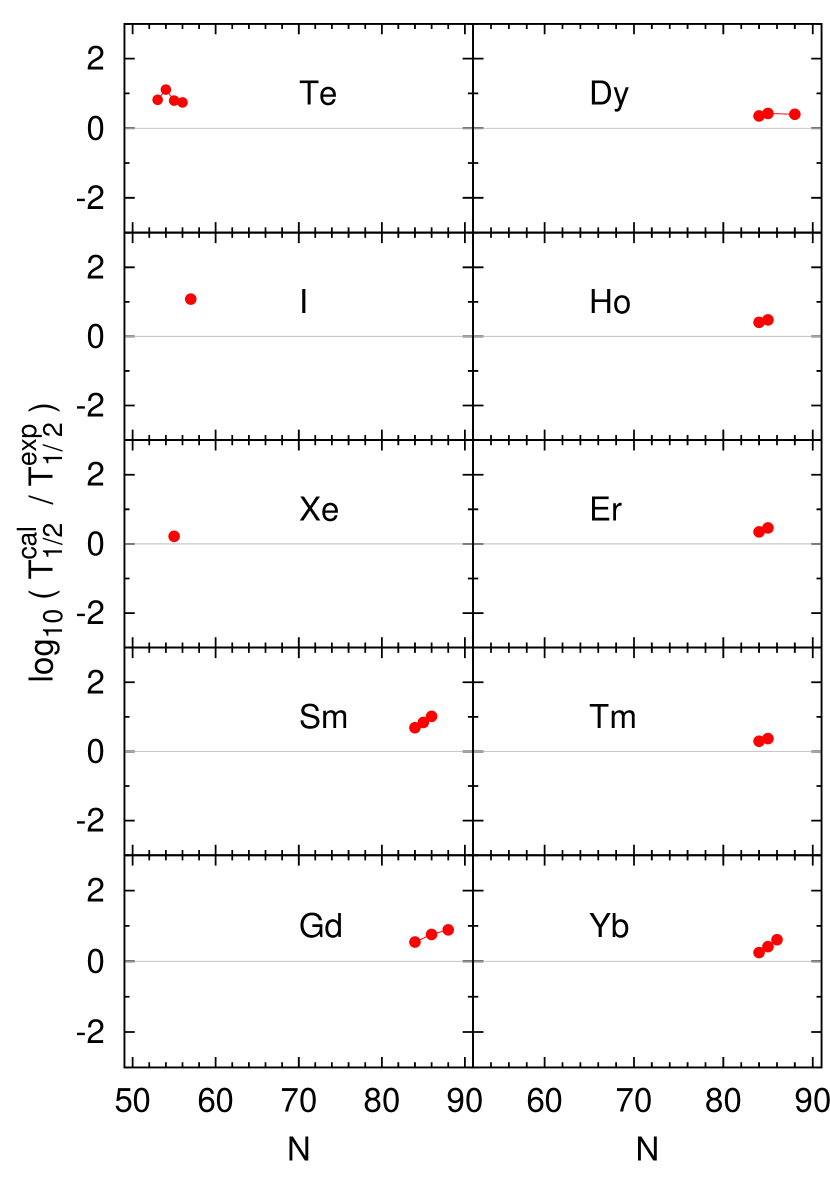
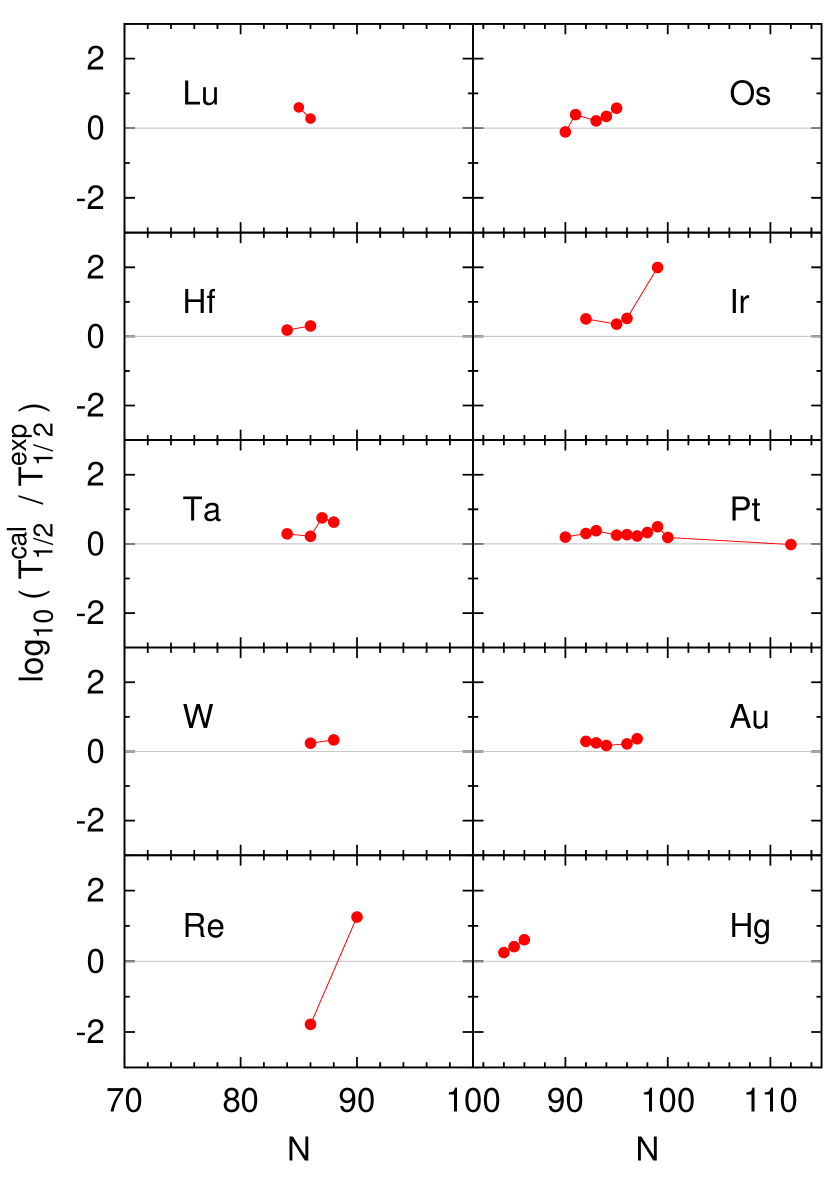
Figure 1: Differences of the theoretical and experimental [11] alpha decay half-lives on logarithmic scale, calculated for nuclei with $52\leq Z\leq 70$ (top) and $71\leq Z\leq 80$ (bottom).

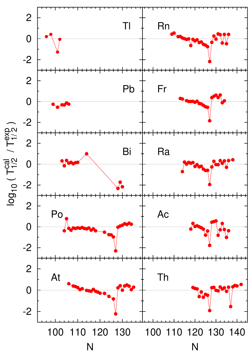
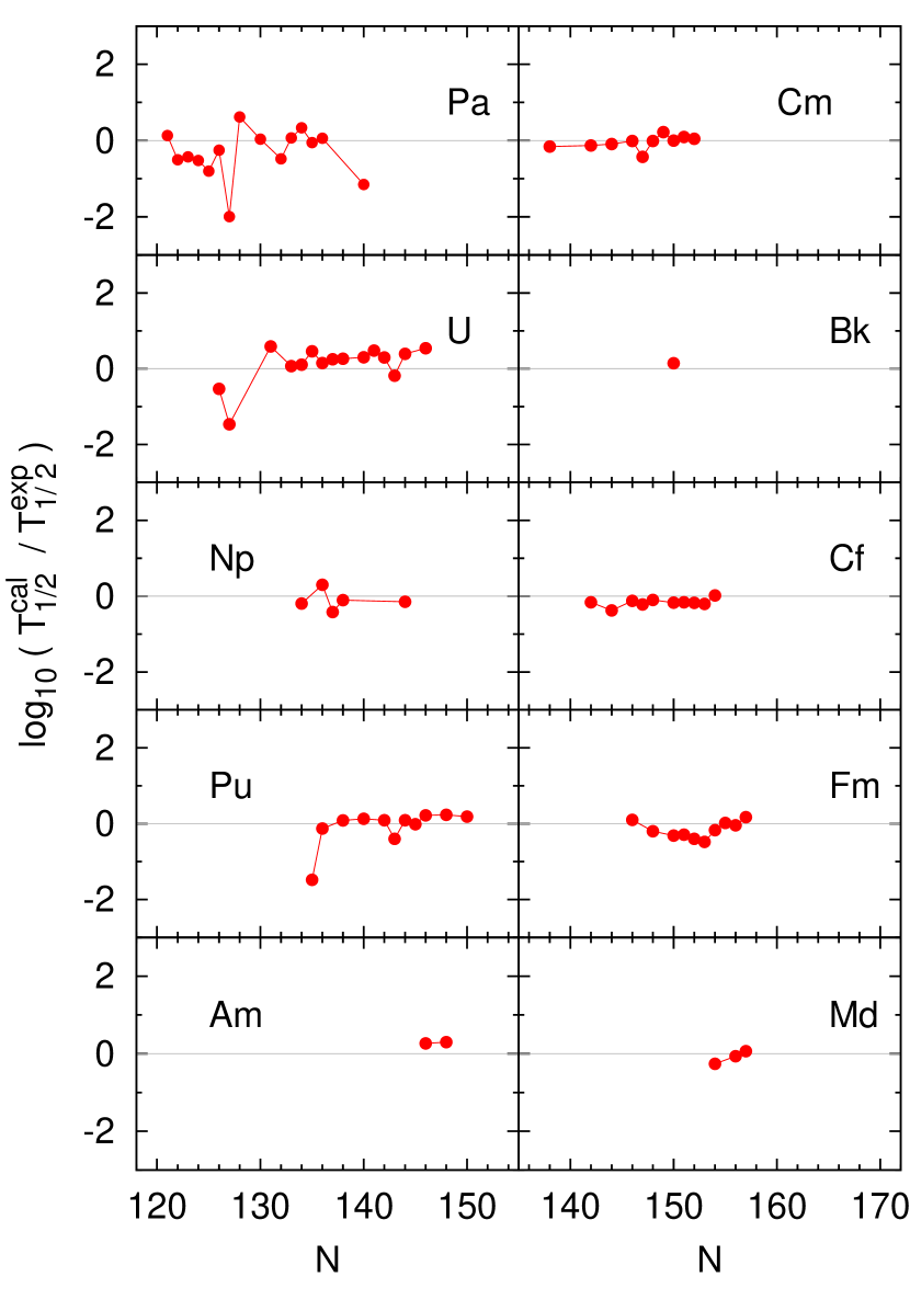
Figure 2: The same as in Fig. 1, but for isotopes with $81\leq Z\leq 90$ (top) and $91\leq Z\leq 101$ (bottom).

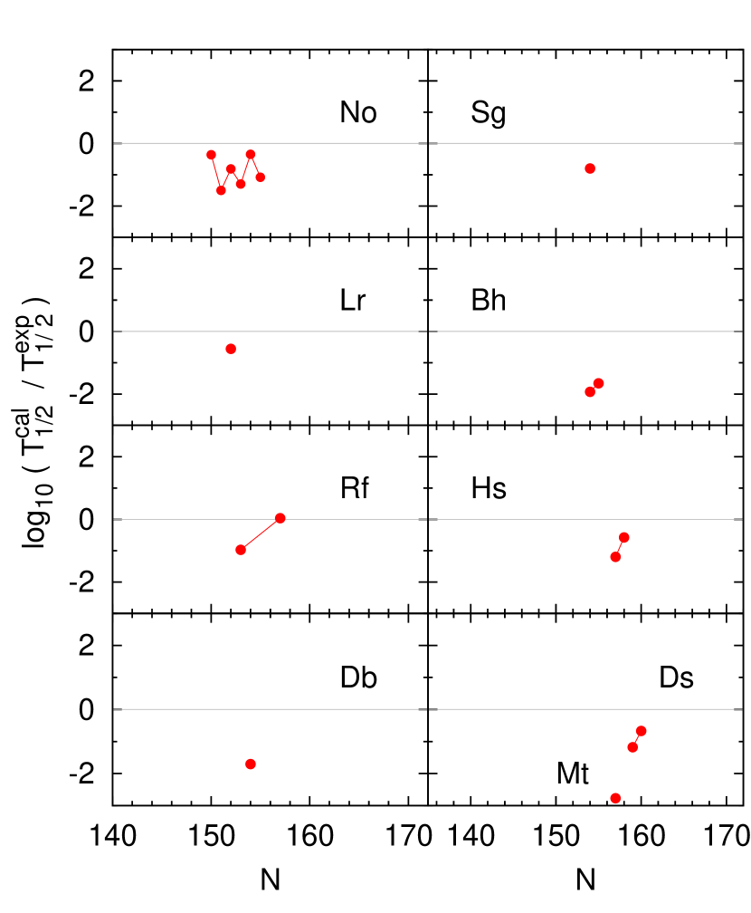
Figure 3: The same as in Fig. 1, but for isotopes with $102\leq Z\leq 110$.

where $\mu$ is a reduced mass, $R$ is the spherical square well radius

$$R=r_{0}(A_{\alpha}^{1/3}+A_{d}^{1/3})$$ (3)

and $b$ is the exit point from the Coulomb barrier:

$$b=\frac{Z_{\alpha}Z_{d}e^{2}}{E_{\alpha}}~{}.$$ (4)

$A_{\alpha},Z_{\alpha}$ and $A_{d},Z_{d}$ are the mass and proton numbers of an alpha particle (or cluster) and a daughter nucleus respectively. $E_{\alpha}$ is the kinetic energy of emitted alpha (cluster) particle [11]. The number of assaults per time-unit $n$ is evaluated from the quantum-mechanical ground-state frequency in the spherical square well:

$$n=\frac{\pi\hbar}{2\mu R^{2}}\,\,.$$ (5)

In this formalism the $\alpha$-decay half-life can be expressed as follows:

$$T_{1/2}=\frac{\ln 2}{\lambda}10^{h}\,\,,$$ (6)

where constant $h$ (so-called hindrance factor) was additionally introduced for odd nuclei. The least-square fit of the radius constant $r_{0}$ was performed to known experimental half-lives of even-even $\alpha$-emitters (127 cases) [11]. Only the most probable alpha decays mode at each isotope was chosen in our analysis. Obtained in this way value of the nuclear well radius constant is equal to $r_{0}=1.23$ fm, and slightly differs from that reported in Ref. [3], as now more alpha emitters were taken and the cluster decays were not included in our analysis. Fitting procedures of hindrance factor were performed for odd systems with fixed $r_{0}$ value ($h=0.25$ for odd-A and doubled for odd-odd emitters).

2.2 Results

The logarithms of the ratios of the half-lives ($T^{\rm cal}_{1/2}$), calculated using above formalism, to the measured ones ($T^{\rm exp}_{1/2}$) for all examined nuclei are shown in Figs. 1-3 as a function of the neutron number $N$.

Large deviations from the data are observed for emitters with neutron number $N=127$ in ₈₃Bi - ₉₂U elements (Fig. 2), where underestimations of the $\rm log_{10}(T_{1/2})$ reach about two orders of magnitude. Calculated half-lives of some lighter emitters (₅₂Te - ₇₄W) are overestimated, but these discrepancies do not exceed one order of magnitude. The root-mean-square deviations of our estimations made for the $\alpha$-decay half-lives for all considered nuclei are summarized in Table 1.

Table 1: Root-mean-square deviations of $\log_{10}(T_{1/2}^{\alpha})$ calculated using Eq. (6) with the radius constant $r_{0}$=1.23 fm.

$\pi_{Z}-\pi_{N}$	n	h	r.m.s.
e-e	127	0	0.39
e-o	97	0.25	0.66
o-e	82	0.25	0.54
o-o	54	0.5	0.79

3 Spontaneous fission within the WKB theory

A continuous interest in the theoretical description of the fission dynamics is observed since discovery of this phenomenon in 1938. In present Section we are going to concentrate on the spontaneous fission and its description within the WKB theory only. The results presented here will be used to understand, why a simple one parameter (for even-even nuclei) model à la Świa̧tecki [9], described in Section 4, is able to reproduce the spontaneous fission half-lives of all known nuclei with higher accuracy than obtained using more advanced theories.

Quantum mechanically it is possible for a nucleus in its ground state to tunnel the fission barrier. The probability of the barrier penetration depends not only on the height and width of the barrier but also on the magnitude of the collective inertia associated with the fission mode. The calculations of the spontaneous fission half-lives $T_{\rm sf}$ require a careful evaluation of the collective potential energy surface and the collective inertia tensor. Different models, like the macroscopic-microscopic model [12, 13] or the Hartree-Fock-Bogolubov self-consistent theories (see e.g. [14]), can be used to generate the potential energy surfaces. The collective mass parameters one evaluates usually in the cranking approximation [15, 13] or within the Generator Coordinate Method (GCM) with the generalized Gaussian Overlap Approximation (GOA) [16].

Figure 4: A contour plot of the energy surface for ²⁵²Fm is shown in the two-dimensional quadrupole $(\epsilon)$ and hexadecapole $(\epsilon_{4})$ deformation parameter space. The dashed line is the path of steepest descent from the saddle points to the ground state and to the scission line, the thick line is the minimal-action path. After Ref. [17].

The spontaneous fission half–life is given by:

$$T^{\rm sf}_{1/2}=\frac{\ln 2}{nP}\,\,.$$ (7)

Here $n$ is the number of assaults per time unit, associated with the frequency of zero–point vibration of the nucleus in the fission mode direction. The fission barrier penetration probability $P$ might be evaluated within the one-dimensional WKB approximation, what leads to the following expression:

$$P=\frac{1}{1+\exp\{2S(L)\}}\,\,.$$ (8)

The action–integral $S(L)$, calculated along a fission path $L(s)$ in the multi–dimensional space of collective coordinates is given by:

$$S(L)=\int^{s_{2}}_{s_{1}}\left\{{2\over\hbar^{2}}\,B_{\rm eff}(s)[V(s)-E_{\rm gs}]\right\}^{1/2}ds\,\,,$$ (9)

where the integration limits $s_{1}$ and $s_{2}$, correspond to the classical turning points. $E_{\rm gs}$ is the energy of a nucleus in its ground state and $V(s)$ is the collective potential. $B_{\rm ss}(s)$ is an effective inertia tensor in the multi-dimensional space of collective coordinates $\{q_{i}\}$:

$$B_{\rm ss}(s)=\sum_{k,\,l}\,B_{kl}\,{dq_{k}\over ds}{dq_{l}\over ds}.$$ (10)

Figure 5: Collective potential (top) and inertia $B_{\rm eff}$ (bottom) along the static (thick solid line) and the dynamic (thin solid line) path to fission as a function of the relative distance between the fragment mass centres $s=R_{12}/R_{0}$. The reduced ($\mu$), irrotational flow and phenomenological inertias [19] are shown for comparison. After Ref. [20].

Figure 6: Spontaneous fission half-lives of even-even transactinides and their shape isomers (II) obtained with the WKB approximation (8) along the least action (dynamical trajectory). After Ref. [18].

Determination of the fission path in the deformation space plays crucial role during evaluation of the fission probability [13]. The action integral (9) should be calculated along such a path (so-called dynamic), which minimize its total value, thereby maximize fission probability (8) [18]. In contrast to the static path, the dynamic one (dependent on the inertia tensor) does not have to lead through the bottom of the fission valley, as one can see in Fig. 4. The comparison of the fission barrier and effective inertia, corresponding to the dynamic and static fission paths for ²⁵⁰Fm is shown in Fig. 5. The collective potential $V(s)$, corresponding to the dynamic path, is larger than in case of the static one, but the dynamic inertia is smaller. It might be roughly approximated by the so-called phenomenological inertia fitted to the observed spontaneous fission half-lives [19]:

$${\cal M}^{\rm phen}_{R_{12}R_{12}}=\mu\left(1+k\frac{17}{15}\exp\left[-a(R_{12}-\frac{3}{4})\right]\right)\,\,.$$ (11)

Here $\mu$ is the reduced mass, corresponding to the relative distance between fragments ($R_{12}$=3/4 for a sphere) and $a=2.452$ is a numerical constant, determined from a fit to the exact irrotational flow inertia [21] for $k=1$. It was found in Ref. [19] that the phenomenological inertia obtained with the constant $k=11.5$ reproduces well the systematics of the known spontaneous fission half-lives.

Spontaneous fission half-lives of even-even transactinides evaluated in Ref. [18] are presented in Fig. 6. The estimates correspond to the least-action trajectories (dynamic path to fission). The WKB approximation (8) and the cranking inertia tensor were used. The two-dimensional potential energy surfaces for each isotope were obtained within the macroscopic-microscopic model using the Nilsson potential and the droplet energy for the macroscopic part. The effects of the axial asymmetry as well as the reflection asymmetry were taken into account.

Usually calculations of spontaneous fission half-lives are performed with an assumption, that the collective potential is equal to the Hartree-Fock-Bogolubov (HFB) binding energy or its macroscopic-microscopic approximation. The zero-point energy corrections are often neglected in papers dealing with similar problems. We shell discuss this point later. Moreover, one assumes, that the ground state is located at $\Delta E\approx 0.5$ MeV above the minimum of the HFB potential. As a justification of such a choice of $\Delta E$ one refers to experimental values of the average quadrupole phonon energy, which is about 1 MeV for actinides. Several authors even treat $\Delta E$ as a free parameter. It should be stressed, that the HFB theory, as each variational method, gives the upper limit of the ground-state energy, so the zero-point correction energy at the equilibrium point is approximately equal to the difference of the ground-state and the potential energy at the minimum (see Ref. [23]). It can be easily shown, that the zero-point energy of harmonic oscillations is equal to the half of the corresponding phonon energy, i.e. ($\frac{1}{2}\hbar\omega$) [24], what is consistent with result, obtained in Ref. [25], where the coupled quadrupole and octupole vibrations in the region of Ra–Th nuclei were analyzed. This conclusion is also valid even for strongly anharmonic motion such as pairing vibrations [26].

The number ($n$) of the collective degrees of freedom results much on the value of the zero-point energy correction. Namely, the $\varepsilon_{0}$ is proportional to $n\cdot\hbar\omega$. Thus, when the HFB equations are solved in the whole $n$-dimensional space of collective coordinates, all zero-point corrections should be substracted from the energy to obtain the collective potential:

$$V(s)=E_{\rm HFB}(s)-\varepsilon_{0}^{\rm fiss}(s)\,\,,$$ (12)

where $\varepsilon_{0}^{\rm fiss}$ is the zero-point energy related to the fission mode [16].

In the case of the one dimensional fission barrier penetration given by the Eq. (9), the oscillations perpendicular to the fission path are not included during evaluation of tunnelling probability (16). In this direction the zero-point energy corrections will be approximately cancelled by the 1/2 of the corresponding phonon energy.

In Fig. 7 the potential and the binding energy along the fission path are plotted. As one can observe, the zero-point corrections may affect on the fission barrier height.

Figure 7: Collective potential $V(s)$, binding energy $E_{\rm HFB}(s)$ and ground-state energy $E_{\rm gs}$ of a nucleus along the fission path $s$. After Ref. [20].

The determination of the least action path in deformation space is not a trivial task (see Ref. [13] for further discussion). The approach, which is worth to be mentioned in this context is dynamical programming method  [17, 18]. Nevertheless, applying this method one should choose optimal distance between the mesh points to avoid large numerical errors. That is because the accuracy of calculations of the partial derivatives $\frac{\partial q_{i}}{\partial s}$, which result much on the effective mass parameter (10) as well as the zero-point energy correction (see e.g. Ref. [16]) along the fission path, strongly depends on the grid size. The von Ritz implementation (see appendix of Ref. [27]) might be useful as an alternative for practical calculations of the spontaneous fission probability. The main advantage of this method is that the influence of the zero-point energy correction along the dynamical paths might easy be taken into account.

Typically the mass yield of the spontaneous fission fragments of the actinide nuclei is spread between 70 and 180. Usually, except the bimodal fission of ²⁵⁸Fm and neighbouring nuclei, the asymmetric fission is more probable than the symmetric one and the most populated mass of the heavier fragment is around 140. A very mass asymmetric spontaneous fission process, when the mass of the lighter fragment is around 20, is already considered as a cluster emission. This type of radioactivity was predicted in 1980 by Sandulescu and co-workers [28] and four years later it was discovered by Rose and Jones [29], who observed the spontaneous emission of ¹⁴C from ²²³Ra. The cluster emission is a very rare process. Its relative branching ratio to the $\alpha$-decay is of the order $10^{-10}$ to $10^{-17}$. Nevertheless, in last two decades one has observed clusters from ¹⁴C to ³⁴Si emitted by actinide nuclei from ²²¹Fr to ²⁴²Cm. In all cases the residual nucleus was always close to the double magic ²⁰⁸Pb.

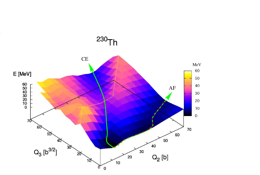
Figure 8: The HFB potential energy of ²³⁰Th as a function of quadrupole and octupole moments. The the thick solid line show the path to cluster emission (CE) while the dashed one is drawn along the valley to asymmetric fission (AF). After Ref. [30].

In general, there are two alternative theoretical descriptions of the spontaneous cluster decay. One can use a fission-like mechanism to reproduce the main features of the process [28, 31, 32, 33, 30] or one assumes, in close analogy to the $\alpha$-decay, that a cluster, performed by a nonadiabatic mechanism inside nucleus, penetrates the potential barrier created by the Coulomb and nuclear interaction with a daughter nucleus [34, 35, 36, 37]. The potential energy landscape of ²³⁰Th obtained by the HFB calculation with the Gogny D1S force [30] is presented in Fig. 8 as a function of quadrupole ($Q_{2}$) and octupole ($Q_{3}$) moments. Two valleys leading to the cluster emission (CE, solid line) and to the asymmetric fission (AF, dashed line) are visible in the plot.

The above theoretical models, which describe the cluster-radioactivity, are rather complex and contain adjustable parameters. Last year we have shown in Ref. [3], that within a simple Gamow model with only one adjustable parameter (radius constant) common for the $\alpha$-decay and the cluster emission one can describe with good accuracy the experimental systematics of half-lives for the cluster radioactivity of even-even nuclei. An additional hindrance constant was introduced in Ref. [3] to describe the cluster emission probability from odd-even, even-odd and odd-odd isotopes.

4 Simple phenomenological formula for the spontaneous fission half-lives

Encouraged by the good result for $T_{1/2}^{\alpha}$ obtained in the Gamow theory, we are going in the following to describe in another simple model the spontaneous fission half-lives of transactinide nuclei. Namely, we shall adopt the Świa̧tecki idea from 1955 [9], who found a simple relation between the spontaneous fission half-lives and the experimental mass deviations from their liquid drop estimates. The crucial ingredient of the model is the liquid drop formula which is described in the next subsection.

4.1 The liquid drop model

In our analysis we decided to use the modern version of the macroscopic-microscopic model [10]. The macroscopic part of this Lublin-Strasbourg Drop (LSD) mass formula (in MeV units) is as follows:

$$\begin{array}[]{l}M_{\rm LSD}(Z,N,{\rm def})=\\[2.15277pt] ~{}~{}7.289034\cdot Z+8.071431\cdot N-0.00001433\cdot Z^{2.39}\\[2.15277pt] ~{}-15.4920(1-1.8601I^{2})A\\[2.15277pt] ~{}+16.9707(1-2.2938I^{2})A^{2/3}\,B_{\rm surf}({\rm def})\\[2.15277pt] ~{}+3.8602(1+2.3764I^{2})A^{1/3}\,B_{\rm cur}({\rm def})\\[2.15277pt] ~{}+0.70978\,Z^{2}/A^{1/3}\,B_{\rm Coul}({\rm def})-0.9181\,Z^{2}/A\\[2.15277pt] ~{}-10\exp({-4.2|I|})\,B_{\rm cong}({\rm def})+E_{\rm o-e}\,\,.\end{array}$$ (13)

where the odd-even energy term $E_{\rm e-o}$ is given in Ref. [38]. In Eq. (13) $A=Z+N$ denotes the mass number, $I=(N-Z)/A$ reduced isospin and $B_{\rm surf}$, $B_{\rm cur}$, $B_{\rm Coul}$ and $B_{\rm cong}$ are relative to the sphere: surface, curvature, Coulomb and congruence (see Ref. [38]) energies. The parameters in the first and the last row in Eq. (13) are taken from Ref. [39], while the rest 8 parameter were fitted to the data.

4.2 Simple model à la Świa̧tecki

Following the idea presented in Ref. [9], we are going to find an approximative functional dependence of the logarithms of spontaneous fission half-lives, corrected by mass shifts $k\delta M$, on proton $Z$ and neutron $N$ numbers:

$$f(Z,N)=\log_{10}[T_{1/2}^{\rm sf}/y]+k\delta M(Z,N)\,\,.$$ (14)

The $\delta M$ is a ground-state microscopic energy, defined as:

$$\delta M_{micr}^{\rm exp}(Z,N)=M_{\rm exp}(Z,N)-M_{\rm LSD}(Z,N,0),$$ (15)

where $M_{\rm exp}(Z,N)$ is a measured mass of isotope, taken from [40] and $M_{\rm LSD}(Z,N,0)$ were calculated using formula (13).

Figure 9: Logarithms of the observed spontaneous fission half-lives corrected with masses ”shifts” $k\delta M$ as a function of proton number.

Fitting procedures included 35 fissioning even-even isotopes ($Z\leq 102$) with measured masses and half-lives. The smooth dependence for even-even isotopes was achieved for factor $k=7.7\,\rm MeV^{-1}$, as it is shown in Fig. 9. The curves, fitted for odd-$A$ and odd-odd nuclei are shifted by a constant- hindrance factor. It is equal to $h=2.5$ for odd-$A$ isotopes and doubled for odd-odd systems. Formula for spontaneous fission half-lives in years is given by:

$$\begin{array}[]{l}\log_{10}\left(\frac{T_{1/2}^{\rm sf}}{y}\right)=-4.1\cdot{\rm min}(Z,103)+380.2\\ ~{}~{}~{}-7.7\,\delta M(Z,N)+\left\{\begin{array}[]{ll}0&{\rm~{}for~{}even-even\,\,,}\\ 2.5&{\rm~{}for~{}odd-}A\,\,,\\ 5&~{}{\rm for~{}odd-odd\,\,.}\end{array}\right.\end{array}$$ (16)

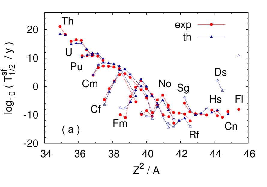
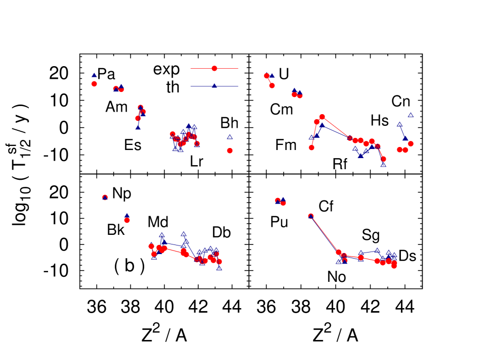
Figure 10: Spontaneous fission half-lives of even-even (a) and odd (b) nuclei, calculated using formula (16) (triangles) in comparison to the experimental values [11] (dots).

Spontaneous fission half-lives, calculated using formula Eq. (16) are presented and compared with the data in Fig. 10. Isotopes which for masses are still not measured are marked with open symbols. A very good accuracy was achieved in actinides region, where the root-mean-square deviation of $\log T_{1/2}^{\rm sf}$ is equal to 1.18 and it grows to 1.57 when odd-$A$ and odd-odd nuclei are taken into account. The r.m.s. deviation reaches 1.96, when one includes to the analysis the super-heavy isotopes, for which the liquid drop barrier vanishes. The quality of reproduction of known life-times by this simple model is even better than that presented in Fig. 6 obtained in the macroscopic-microscopic model with the cranking inertia [18]. Also more advanced modern calculations based on the HFB theory with the Skyrme (see e.g. [41, 42] or Gogny force [43] did not bring better estimates for large sample of isotopes than the simple formula presented above. It raises a question: why the simple Świa̧tecki model works? To understand it, one has to recall Świa̧tecki’s topographical theorem and the results obtained using dynamic (least action) trajectories to fission described in Section 3.

4.3 The topographical theorem

Figure 11: Experimental fission barrier heights compared with their estimates evaluated according to the topographical theorem of Świa̧tecki and the LSD macroscopic energy. After Ref. [46].

It was shown in Refs. [10, 27, 44] that the LSD model (13), which parameters were fitted to the experimental ground-state masses only, is able to reproduce well the fission barrier heights of light, medium and heavy nuclei, when the microscopic part of the ground-state binding energy is taken into account. According to the topographical theorem, proposed by Myers and Świa̧tecki [38], the mass of a nucleus in a saddle-point is mostly determined by the macroscopic part of its binding energy. The influence of the shell effects on the saddle-point energy is rather weak and in the first approximation might be neglected. So, one can evaluate the fission barrier height as a difference between the macroscopic (here LSD) and the experimental mass:

$$V_{B}(Z,N)=M_{\rm LSD}(Z,N,{\rm saddle})-M_{\rm exp}^{g.s.},$$ (17)

where $M_{\rm LSD}(Z,N,{\rm saddle})$ is a macroscopic part of LSD mass formula (13) taken in a saddle point.

The comparison of the experimental fission barrier height of actinide nuclei with their estimates, evaluated according to the topographical theorem of Świa̧tecki using the LSD macroscopic energy, is presented in Fig. 11. The r.m.s. deviation of the estimates from the data for all 18 considered fission barriers heights is 0.31 MeV only, what proves, that the topographical theorem really works [46]. All estimates do not exceed 0.67 MeV and lie below the experimental values (except ²⁵⁰Cf), what give a place for not washed out shell effects around the saddle point energy.

4.4 Justification of the simple formula for $T_{\rm sf}$

Let us consider one dimensional fission barrier along the least-action (dynamic) trajectory described in Sec. 3. Assuming, that the fission path is parametrised by the collective coordinate $s$, one can evaluate the potential $V(s)$ and the mass parameter $B_{ss}(s)$ corresponding to this path. The fluctuations of the inertia $B_{ss}$ along the least-action trajectory becomes smaller and smaller, when one increase the number of collective coordinates. Especially the collective pairing degrees of freedom significantly wash out the fluctuations of the inertia function [47].

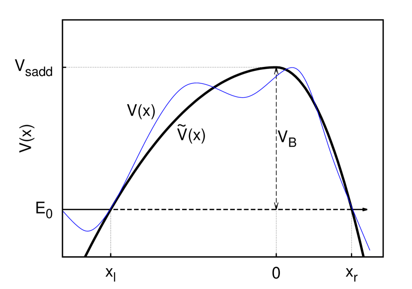
Figure 12: Schematic plot of a fission barrier in form of two inverted parabolas smoothly joined at the scission point.

A simple transformation:

$$x(s)=\int\limits_{s_{\rm sadd}}^{s}\sqrt{\frac{B_{s}s(s^{\prime})}{m}}ds^{\prime}\,\,,$$ (18)

bring us to the new coordinate $x(s)$, in which the inertia becomes constant $B_{xx}=m$. The lower integration limit in Eq. (18) is chosen at point $x=0$, corresponding to the saddle point $s_{\rm sadd}$. The collective potential in the new coordinate, schematically plotted in Fig. 12, can be approximated by two inverted parabolas of different stiffnesses $C_{l}$ and $C_{r}$ having the maximum at the saddle point:

$$\widetilde{V}(x)=\left\{\begin{array}[]{ll}V_{\rm sadd}-\frac{1}{2}\,C_{l}\,x^{2}{}{}{}&{\rm for}~{}~{}~{}x\,<\,0\,\,,\\[4.30554pt] V_{\rm sadd}-\frac{1}{2}\,C_{r}\,x^{2}{}{}{}&{\rm for}~{}~{}~{}x\,>\,0\,\,,\end{array}\right.$$ (19)

The stiffnesses of the $\widetilde{V}$ potential are chosen in such a way that the action-integral $S$ (9) becomes equal:

$$\int\limits_{-x^{\prime}_{l}}^{x^{\prime}_{r}}\!\!\sqrt{\frac{2m}{\hbar^{2}}[V(x)-E_{0}]}\,dx=\!\!\int\limits_{-x_{l}}^{x_{r}}\!\!\sqrt{\frac{2m}{\hbar^{2}}[\widetilde{V}(x)-E_{0}]}\,dx$$ (20)

where pairs ($-x^{\prime}_{l},x^{\prime}_{r}$) and ($-x_{l},x_{r}$) are classical left and right turning points for the true and approximative potential respectively. The last integral in Eq. (20) can be rewritten as

$$S=\!\sqrt{\frac{2m}{\hbar^{2}}}\left\{\!\int\limits_{0}^{x_{l}}\!\sqrt{V_{B}-\frac{C_{l}x^{2}}{2}}\,dx+\!\!\int\limits_{0}^{x_{r}}\!\sqrt{V_{B}-\frac{C_{r}x^{2}}{2}}\,dx\right\},$$

where $V_{B}=V_{\rm sadd}-E_{0}$ is the fission barrier height.
After a small algebra the action integral becomes

$$S=\frac{\pi}{2\hbar}V_{B}\left(\sqrt{\frac{m}{C_{l}}}+\sqrt{\frac{m}{C_{r}}}\right)=\frac{\pi}{\hbar}V_{B}\frac{\omega_{l}+\omega_{r}}{2\omega_{l}\omega_{r}}\,\,,$$ (21)

where $\omega_{l}=\sqrt{C_{l}/m}$ and $\omega_{r}=\sqrt{C_{r}/m}$ are frequencies of the left and right (inverted) oscillator respectively. Introducing the average oscillator frequency

$$\widetilde{\omega}=\frac{2\omega_{l}\omega_{r}}{\omega_{l}+\omega_{r}}\,,$$ (22)

one can bring the action integral to the following form:

$$S=\frac{2V_{B}}{\hbar\widetilde{\omega}}\,.$$ (23)

In our approximation the action integral is proportional to the fission barrier height measured in the energy quanta of the harmonic oscillator, which approximates the fission barrier form. For the action-integral $S>1$ the logarithm of the spontaneous fission half-lives (7) can written as

$$\log(T^{\rm sf}_{1/2}/y)=2S-\log(n)-0.3665$$ (24)

where the constant 0.3665=log[ln(2)] and $n$ is the number of assaults of nucleus on the fission barrier per year ($y$). Having in mind, that according to the topographical theorem the fission barrier height is $V_{B}=M_{\rm LSD}^{\rm sadd}-M_{exp}^{gs}$ and making use of the relation (23), one can rewrite the last equation as follows:

$$\log(T^{\rm sf}_{1/2}/y)+\frac{4\delta M^{\rm exp}_{\rm micr}}{\hbar\tilde{\omega}}=\frac{4V_{B}^{\rm LSD}}{\hbar\tilde{\omega}}-\log(n)-0.3665~{},$$ (25)

where $\delta M^{\rm exp}_{\rm micr}$ was defined in Eq. (15) and $V_{B}^{\rm LSD}=M_{\rm LSD}^{\rm sadd}-M_{\rm LSD}^{\rm sph}$ is the liquid drop fission barrier height. The right hand side of Eq. (25) is a very smooth function of nucleon numbers as it is defined only by global properties of nucleus. Note, that the derived equation has the same structure as the phenomenological formula of Świa̧tecki (14), what proves his Ansatz.

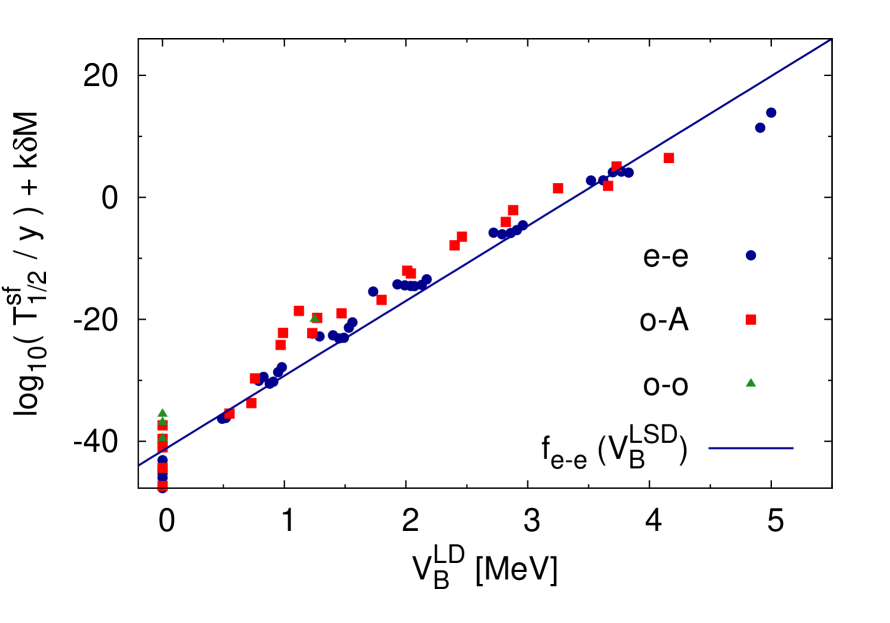
Figure 13: Logarithms of the observed spontaneous fission half-lives corrected with $7.7{\delta M}$ as a function of liquid drop barrier height.

The liquid drop barrier height of actinides decreases almost linearly in function of $Z$ from 4.3 MeV for $Z=90$ to 0 for $Z\geq 103$ [44]. The fission barrier of finite height appears in the super-heavy nuclei mostly due to the shell effects in the ground state. The smooth dependence of logarithms of spontaneous fission half-lives, corrected by the ground state shell-plus-pairing effects, on the LSD fission barrier heights, shown in Fig. 13 for even-even (e-e), odd A (o-A) and odd-odd (o-o) nuclei. The data for e-e isotopes lie very close to the straight line, what validates Eq. (25). The data for o-A and o-o are above this line, what is due to the specialization energy, which increase the fission barrier heights. As it was mentioned before, stability of super-heavy nuclei is determined by shell effects. The liquid drop barrier of these isotopes vanishes, what is visible in Fig. 13 for nuclei with $Z\geq 103$.

5 Conclusions

The following conclusions can be drawn from our investigation:

• Simple, consistent model was applied to reproduce alpha decay half-lives in 360 nuclei with atomic number $52\leq$ Z $\leq 110$.
  

• Model reproduces $\alpha-$decay half-lives with quite good accuracy; the root-mean-square deviation of $\rm log_{10}(T^{\alpha}_{1/2})$ for even-even isotopes is equal to 0.39.
  

• Large underestimations in half-lives of $N=127$ isotones arises from strong shell effects, which are not considered in this simple model.
  

• Semi-empirical formula for the spontaneous fission half-lives, depending on proton number and the ground state microscopic corrections, reproduces data for even-even super-heavy nuclei with reasonable accuracy.
  

• Quality of spontaneous fission half-lives evaluation breaks down for nuclei with not measured yet masses.
  

• The logarithms of the spontaneous fission half-lives, corrected by the ground state shell-plus-pairing effects, are roughly proportional to the macroscopic barrier heights in nuclei up to Z=102.
  

6 Acknowledgements

This work was supported by the Polish National Science Centre grant No. 2013/11/B/ST2/04087.

7 References

References

- [1] Gamow G, Z. Phys. 51, 204 (1928).
- [2] Gurney R, Condon E, Nature 122, 439 (1928).
- [3] Zdeb A, Warda M, Pomorski K, Phys. Rev. C 87, 024308 (2013).
- [4] Parkhomenko A, Sobiczewski A, Acta Phys. Pol. B 36, 3095 (2005).
- [5] Viola V E Jr, Seaborg G T, J. Inorg. Nucl. Chem 28, 741 (1966).
- [6] Hahn O, Straßmann F, Naturwiss. 27, 11 (1939); Naturwiss. 27 89, (1939).
- [7] Meitner L, Frisch O R, Nature 143, 239 (1939).
- [8] Flerov G N, Petrzhak K A, Phys. Rev. 58, 89 (1940); Journ. of Phys. (USSR) 3, 275 (1940).
- [9] Świa̧tecki W J, Phys. Rev. 100, 937 (1955).
- [10] Pomorski K, Dudek J, Phys. Rev. C 67, 044316 (2003).
- [11] http://www.nndc.bnl.gov/nudat2/
- [12] S. G. Nilssen, C. F. Tsang, A. Sobiczewski, Z. Szymanski, S. Wycech, C. Gustafson, I. L. Lamm, P. Möller, and B. Nilsson, Nucl. Phys. A131 1 (1969).
- [13] M. Brack, J. Damgaard, A. S. Jensen, H. C. Pauli, V. M. Strutinsky, and C. Y. Wong, Rev. Mod. Phys. 44 (1972) 320.
- [14] Ripka M, Porneuf M, Nuclear Self Consistent Fields, North Holland, New York, 1975.
- [15] A. Sobiczewski, Z. Szymański, S. Wycech, S.G. Nilsson, J.R. Nix, X.F. Tsang, C. Gustafson, P. Möller and B. Nilsson, Nucl. Phys. A131 67 (1969).
- [16] Góźdź A, Pomorski K, Brack M, Werner E, Nucl. Phys. A442, 26 (1985).
- [17] Baran A, Phys. Lett. 76B, 8 (1978).
- [18] Baran A, Pomorski K, Łukasiak A, Sobiczewski A, Nucl. Phys. A361, 83 (1981).
- [19] Randrup J, Larsson S E, Moeller P, Nilsson S G, Pomorski K, Sobiczewski A, Phys. Rev. C13, 229 (1976).
- [20] Pomorski K, Int. J. Mod. Phys. E17, 245 (2008).
- [21] Fiset E O, Nix J R, Nucl. Phys. A193, 647 (1972).
- [22] Myers W D, Świa̧tecki W J, Nucl. Phys. A 612, 249 (1997).
- [23] Goeke K, Phys. Rev. Lett. 38, 212 (1977).
- [24] Ring P, Schuck P, The Nuclear Many-Body Problem, Springer Verlag, Heidelberg, 1980.
- [25] Robledo L M, Egido J L, Nerlo-Pomorska B, Pomorski K, Phys. Lett. B201, 409 (1988).
- [26] Sieja K, Baran A, Pomorski K, Eur. Phys. Journ. A20, 413 (2004).
- [27] Dobrowolski A, Pomorski K, Bartel J, Phys. Rev. C75, 024613 (2007).
- [28] Sandulescu A, Poenaru D N, Greiner W, Sov. J. Part Nucl. 11, 528 (1980).
- [29] Rose H J, Jones G A, Nature 307, 245 (1984).
- [30] Robledo L M, Warda M, Int. Journ. Mod. Phys. E17, 204 (2008).
- [31] G. A. Pik-Pichak, Sov. J. Nucl. Phys. 44 923 (1986).
- [32] Y.-J. Shi and W. J. Swiatecki, Nucl. Phys. A464 205 (1987).
- [33] Poenaru D N, Gherghescu R A, Greiner w, Phys. Rev. C73, 014608 (2006).
- [34] Kademsky S G, Furman W I, Tchuvilsky W I, Yu M, Izv. Akad. Nauk SSSR, Ser. Fiz. 44, 1786 (1986).
- [35] Gupta R K, Gilaty S, Malik S S et al., J. Phys. G13 L27 (1987).
- [36] Blendowske R, Flissbach T, Walliser H, Nucl. Phys. A464, 75 (1987).
- [37] Blendowske R, Flissbach T, Walliser H, Zeit. Phys. A339, 121 (1990).
- [38] Myers W D, Świa̧tecki W J, Nucl. Phys. A601, 141 (1996).
- [39] Möller P, Nix J R, Myers W D, and Świa̧tecki W J, At. Data Nucl. Data Tables 59, 185 (1995).
- [40] http://amdc.in2p3.fr/nubase/Nubase2012-v3.pdf
- [41] Staszczak A, Baran A, Nazarewicz W, Phys. Rev. C 87, 024320 (2013).
- [42] Sadhukhan J, Mazurek K., Baran A, Dobaczewski J, Nazarewicz W, Sheikh J A, Phys. Rev. C 88, 064314 (2013)
- [43] Rodriguez-Guzman R, Robledo L M, Phys. Rev. C 89, 054310 (2014).
- [44] Ivanyuk F A, Pomorski K, Phys. Rev. C 79, 054327 (2009).
- [45] Krappe H J, Pomorski K, Theory of Nuclear Fission, Springer Verlag, Heidelberg, 2012.
- [46] Dobrowolski A, Nerlo-Pomorska B, Pomorski K, Acta Phys. Pol. B40, 705 (2009).
- [47] Staszczak A, Pilat S, Pomorski K, Nucl. Phys. A504, 589 (1989).