The joint statistics of mildly non-linear cosmological densities and slopes in count-in-cells

Abstract

In the context of count-in-cells statistics, the joint probability distribution of the density in two concentric spherical shells is predicted from first first principle for sigmas of the order of one. The agreement with simulation is found to be excellent. This statistics allows us to deduce the conditional one dimensional probability distribution function of the slope within under dense (resp. overdense) regions, or of the density for positive or negative slopes. The former conditional distribution is likely to be more robust in constraining the cosmological parameters as the underlying dynamics is less evolved in such regions. A fiducial dark energy experiment is implemented on such counts derived from $\Lambda$CDM simulations.

1 Introduction

With the advent of large galaxy surveys (e.g. SDSS and in the coming years Euclid (Laureijs et al., 2011), LSST), astronomers have ventured into the era of statistical cosmology and big data. Hence, there is a dire need for them to build tools that can efficiently extract as much information as possible from these huge data sets at high and low redshift. In particular, this means being able to probe the non-linear regime of structure formation. The most commonly used tools to extract statistical information from the observed galaxy distribution are N-point correlation functions (e.g Scoccimarro et al., 1998) which quantify how galaxies are clustered. In our initially Gaussian Universe the matter density field is fully described by its two-point correlation function. However departure from Gaussianity occurs when the growth of structure becomes non-linear (at later times or smaller scales), providing information that is not captured by the two-point correlation function but is recorded in part in the three-point correlation function. Obviously N-point correlation functions are increasingly difficult to measure when N increases. They are noisy, subject to cosmic variance and highly sensitive to systematics such as the complex geometry of surveys. It is thus essential to find alternative estimators to extract information from the non-linear regime of structure formation in order to complement these classical probes. This is in particular critical if we are to understand the origin of dark energy, which accounts for $\sim$ 70 % of the energy budget of our Universe.

One such method to accurately probe the non-linear regime is to implement perturbation theory in a highly symmetric configuration (spherical or cylindrical symmetry) for which the full joint cumulant generating functions can be constructed. Such constructions take advantage of the fact that non-linear solutions to the gravitational dynamical equations (the so-called spherical collapse model) are known exactly. Corresponding observables, such as galaxy counts in concentric spheres or discs, then yield very accurate analytical predictions in the mildly non-linear regime, well beyond what is usually achievable using other estimators. The corresponding symmetry implies that the most likely dynamical evolution (amongst all possible mapping between the initial and final density field) is that corresponding to the spherical collapse for which we can write an explicit linear to nonlinear mapping. This has been demonstrated in the limit of zero variance using direct diagram resummations (Bernardeau, 1992, 1994) which was later shown to correspond to a saddle approximation (Juszkiewicz et al., 1993; Valageas, 2002; Bernardeau et al., 2014). The key point on which this whole paper is based upon, is that the zero variance limit is shown to provide a remarkably good working model for finite variances (Bernardeau, 1994; Bernardeau et al., 2014).

This formalism also allows to weigh non-uniformly different regions of the universe making possible to take into account the fact that the noise structure in surveys is not homogenous. For instance, low density regions are probed by fewer galaxies. Conversely, on dynamical grounds, we also expect the level of non-linearity in the field to be in-homogenous: low density regions are less non-linear. Hence it is of interest to build statistical estimators which probe the mildly non linear regime and that can be tuned to probe subsets of the field, offering the best compromise between these constraints. In the context of the cosmic density field, the construction of conditional distributions naturally leads to the elaboration of joint probability distribution functions (PDF hereafter) of the density in concentric cells.

Following Bernardeau et al. (2014) (hereafter BPC), we propose in Section 2 to extend one-point statistics of density profiles and to the full joint probability distribution function of the density in two concentric spheres of different radii. This is obtained using perturbation theory core results on the cumulant generating function, the double inverse Laplace transform of which is then computed from brute force numerical integration. From that PDF, we will also present the statistics of density profiles restricted to underdense (resp. overdense) regions, and the statistics of density restricted to positive (resp. negative) slopes (Section 3). Theoretical predictions will be shown to be in very good agreement with simulations in the mildly non-linear regime. Dependence with redshift will also be discussed. Finally Section 4 presents a simple fiducial dark energy experiment, while 5 wraps up.

2 The 2-cell density statistics

For the sake of clarity, let us present and briefly comment the formalism. We consider two spheres ${\cal S}_{i}$ of radius $R_{i}$ ($i=1,2$) centered on a given location of space $\textbf{x}_{0}$. Our goal is to derive the joint PDF of the density in ${\cal S}_{1}$ and ${\cal S}_{2}$ denoted ${\hat{\rho}}_{i}$ and rescaled so that $\left\langle{\hat{\rho}}_{i}\right\rangle=1$.

2.1 The cumulant generating function

In the cases we are interested in, the joint statistical properties of ${\hat{\rho}}_{1}$ and ${\hat{\rho}}_{2}$ are fully encoded in their moment generating function

$${\cal M}_{R_{1}R_{2}}(\lambda_{1},\lambda_{2}) = \sum_{p,q=0}^{\infty}\ \langle{\hat{\rho}}_{1}^{p}{\hat{\rho}}_{2}^{q}\rangle\frac{\lambda_{1}^{p}\lambda_{2}^{q}}{p!\,q!}\,,$$ (1)

$$= \langle\exp(\lambda_{1}{\hat{\rho}}_{1}+\lambda_{2}{\hat{\rho}}_{2})\rangle\,,$$ (2)

that can be related to the cumulant generating function, $\varphi_{R_{1}R_{2}}(\lambda_{1},\lambda_{2})$, through ${\cal M}_{R_{1}R_{2}}(\lambda_{1},\lambda_{2})=\exp\left[\varphi_{R_{1}R_{2}}(\lambda_{1},\lambda_{2})\right]$, so that

$$\exp\left[\varphi_{R_{1}R_{2}}(\lambda_{1},\lambda_{2})\right]$$ (3)

$$=\int\hbox{d}{\hat{\rho}}_{1}\hbox{d}{\hat{\rho}}_{2}{\cal P}_{R_{1}R_{2}}({\hat{\rho}}_{1},{\hat{\rho}}_{2})\exp(\lambda_{1}{\hat{\rho}}_{1}+\lambda_{2}{\hat{\rho}}_{2}),$$

where ${\cal P}_{R_{1}R_{2}}({\hat{\rho}}_{1},{\hat{\rho}}_{2})$ is the joint PDF of having density ${\hat{\rho}}_{1}$ in ${\cal S}_{1}$ and ${\hat{\rho}}_{2}$ in ${\cal S}_{2}$. We will now exploit a theoretical construction that permits the explicit calculation of ${\cal P}_{R_{1}R_{2}}({\hat{\rho}}_{1},{\hat{\rho}}_{2})$.

2.1.1 Upshot

As we will sketch in the following, this theoretical construction yields the explicit time dependence of the Legendre transform of $\varphi_{R_{1}R_{2}}(\lambda_{1},\lambda_{2})$ in the quasi-linear regime. Such a Legendre transform is defined as

$$\Psi_{R_{1}R_{2}}(\rho_{1},\rho_{2})=\lambda_{1}\rho_{1}+\lambda_{2}\rho_{2}-\varphi_{R_{1}R_{2}}(\lambda_{1},\lambda_{2}),$$ (4)

where $\rho_{i}$ are determined implicitly by the stationary conditions

$$\lambda_{i}=\frac{\partial}{\partial\rho_{i}}\Psi_{R_{1}R_{2}}(\rho_{1},\rho_{2})\,,\quad{i=1,2}\,.$$ (5)

The fundamental relation is then that, in the limit of zero variance, this Legendre transforms taken at two different times, $\Psi(\rho_{1},\rho_{2};\eta)$ and $\Psi^{\prime}(\rho_{1},\rho_{2};\eta^{\prime})$, take the same value

$$\Psi_{R_{1}R_{2}}(\rho_{1},\rho_{2};\eta)=\Psi_{R^{\prime}_{1}R^{\prime}_{2}}(\rho^{\prime}_{1},\rho^{\prime}_{2};\eta^{\prime})\,,$$ (6)

provided that $\rho_{i}R_{i}^{3}=\rho^{\prime}_{i}{R^{\prime}_{i}}^{3}$, and that $\rho^{\prime}_{i}$ and $\rho_{i}$ are linked together through the nonlinear dynamics of spherical collapse.

Equation (6), when applied to an arbitrarily early time $\eta^{\prime}$, yields a relation between $\Psi(\rho_{1},\rho_{2};\eta)$ and the statistical properties of the initial density fluctuations. In particular, for Gaussian initial conditions, $\Psi(\rho_{1},\rho_{2};\eta_{i})$ can easily be calculated and expressed in terms of elements of covariance matrices,

$$\Psi_{R_{1}R_{2}}(\rho_{1},\rho_{2};\eta_{i})=\frac{1}{2}\sum_{i,j\leq 2}\Xi_{ij}(\rho_{i}-1)(\rho_{j}-1)\,,$$ (7)

where $\Xi_{ij}$ is the inverse of the matrix of covariances, $\Sigma_{ij}=\langle\tau_{i}\tau_{j}\rangle$, between the initial density contrasts in the two concentric spheres of radii $R_{i}$. One can then write the cumulant generating function at any time through the spherical collapse mapping between one final density at time $\eta$ in a sphere of radius $R_{i}$ and one initial contrast in a sphere centered on the same point and with radius $R^{\prime}_{i}=R_{i}\rho_{i}^{1/3}$ (so as to encompass the same total mass); it can be written formally as

$$\rho_{i}=\zeta_{\rm SC}(\eta,\tau_{i})\approx\frac{1}{(1-D_{+}(\eta)\tau/\nu)^{\nu}}\,,$$ (8)

where, for the sake of simplicity, we use here a simple prescription, with $D_{+}(\eta)$ the linear growth factor and $\nu=21/13$ to reproduce the high-z skewness.

Recall that only $\Psi_{R_{1}R_{2}}(\rho_{1},\rho_{2})$ is easily computed. The statistically relevant cumulant generating function, $\varphi_{R_{1}R_{2}}(\lambda_{1},\lambda_{2})$, is only accessible via equation (4) through an inverse Legendre transform which brings its own complications. In particular note that all values of $\lambda_{i}$ are not accessible due to the fact that the $\rho_{i}$ – $\lambda_{i}$ relation cannot always be inverted. This is signaled by the fact that the determinant of the transformation vanishes, e.g. ${\rm Det}\left[{\partial\rho_{i}\partial\rho_{j}}\Psi(\rho_{1},\rho_{2})\right]=0$. This condition is met both for finite values of $\rho_{i}$ and $\lambda_{i}$. The corresponding contour lines of $\varphi(\lambda_{1},\lambda_{2})$ was investigated in BPC and successfully compared to simulation.

2.1.2 Motivation

It is beyond the scope of this letter to re-derive equations (4)-(6) - a somewhat detailed presentation can be found in Valageas (2002) and in Bernardeau et al. (2014) - but we can give a hint of where it comes from: it is always possible to express any ensemble average in terms of the statistical properties of the initial density field so that we can formally write

$$\hskip-2.84544pt\exp\left[\varphi\right]\!\!=\!\!\int\!\!{\cal D}\tau_{1}{\cal D}\tau_{2}\,{\cal P}(\tau_{1},\tau_{2})\exp\big{(}\lambda_{1}\rho_{1}(\tau_{1})+\lambda_{2}\rho_{2}(\tau_{2})\big{)}\,.\hskip-8.5359pt$$ (9)

As the present-time densities $\rho_{i}$ can arise from different initial contrasts, the above-written integration is therefore a path integral (over all the possible paths from initial conditions to present-time configuration) with measure ${\cal D}\tau_{1}{\cal D}\tau_{2}$ and known initial statistics ${\cal P}(\tau_{1},\tau_{2})$. Let us assume here that the initial PDF is Gaussian so that,

$${\cal P}(\tau_{1},\tau_{2})\hbox{d}\tau_{1}\hbox{d}\tau_{2}=\frac{\sqrt{\det\Xi}\exp\left[-\Psi(\tau_{1},\tau_{2})\right]}{2\pi}\hbox{d}\tau_{1}\hbox{d}\tau_{2}\,,$$ (10)

with $\Psi$ then a quadratic form.

In the regime where the variance of the density field is small, equation (9) is dominated by the path corresponding to the most likely configurations. As the constraint is spherically symmetric, this most likely path should also respect spherical symmetry. It is therefore bound to obey the spherical collapse dynamics. Within this regime equation (9) becomes

$$\hskip-2.84544pt\exp\left[\varphi\right]\!\!\simeq\!\!\int\!\!d\tau_{1}d\tau_{2}\,{\cal P}(\tau_{1},\tau_{2})\exp\big{(}\lambda_{1}\zeta_{{\rm SC}}(\tau_{1})\!+\!\lambda_{2}\zeta_{{\rm SC}}(\tau_{2})\big{)},\hskip-12.80365pt$$ (11)

where the most likely path, $\rho_{i}=\zeta_{\rm SC}(\eta,\tau_{i})$ is the one-to-one spherical collapse mapping between one final density at time $\eta$ and one initial density contrast as already described. The integration on the r.h.s. of equation (11) can now be carried by using a steepest descent method, approximating the integral as its most likely value, where $\lambda_{1}\rho_{1}(\tau_{1})+\lambda_{2}\rho_{2}(\tau_{2})-\Psi(\tau_{1},\tau_{2})$ is stationary. It eventually leads to the fundamental relation (6) when its right hand side is computed at initial time (and the fact that (6) is valid for any times $\eta$ and $\eta^{\prime}$ is obtained when the same reasoning is applied twice, for the two different times).

The purpose of this letter is to confront numerically computations of the two-cell PDF derived from the expression of $\varphi(\lambda_{1},\lambda_{2})$ with measurements in numerical simulations.

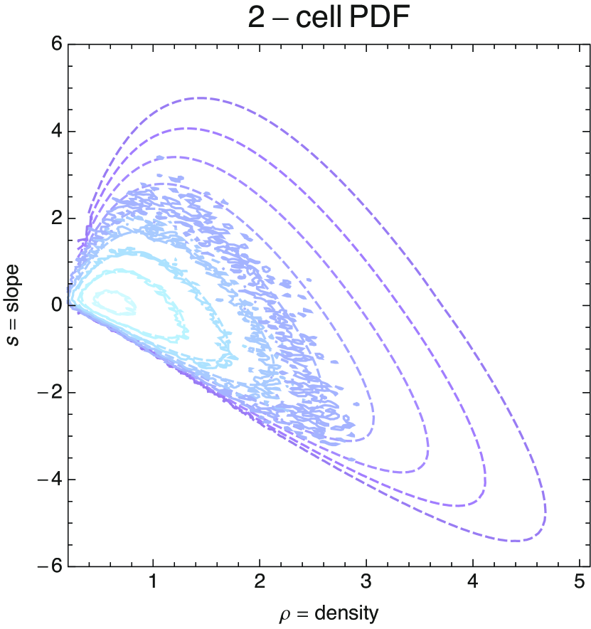
Figure 1: Joint PDF of the slope ($s$) and the density ($\rho$) as given by equation (13) for two concentric spheres of radii $R_{1}=10$ Mpc/h and $R_{2}=11$ Mpc/h at redshift $z=0.97$. Dashed contours corresponds to Log ${\cal P}=0,-1/2,-1,\cdots-3$ for the theory. The corresponding measurements are shown as a solid line.

2.2 The 2-cell PDF using inverse Laplace transform

Once the cumulant generating function is known in equation (3), the 2-cell PDF, ${\cal P}(\hat{\rho}_{1},\hat{\rho}_{2})$, is obtained by a 2D inverse Laplace transform of $\varphi(\lambda_{1},\lambda_{2})$

$${\cal P}\!=\!\!\int_{-\hbox{i}\infty}^{\hbox{i}\infty}\!\!\frac{\hbox{d}\lambda_{1}}{2\pi\hbox{i}}\int_{-\hbox{i}\infty}^{\hbox{i}\infty}\!\!\frac{\hbox{d}\lambda_{2}}{2\pi\hbox{i}}\exp(-\!\!\sum_{i=1,2}\hat{\rho}_{i}\lambda_{i}+\varphi(\lambda_{1},\lambda_{2}))\,,$$ (12)

with $\varphi$ given by equations (4)-(6). From this equation, it is straightforward to deduce the joint PDF, $\hat{\cal P}(\hat{\rho},\hat{s})$, for the density, ${\hat{\rho}}={\hat{\rho}}_{1}$ and the slope $\hat{s}\equiv({\hat{\rho}}_{2}-{\hat{\rho}}_{1})R_{1}/\Delta R$, $\Delta R$ being $R_{2}-R_{1}$, as

$$\hat{\cal P}=\int_{-\hbox{i}\infty}^{\hbox{i}\infty}\frac{\hbox{d}\lambda}{2\pi\hbox{i}}\int_{-\hbox{i}\infty}^{\hbox{i}\infty}\frac{\hbox{d}\mu}{2\pi\hbox{i}}\exp(-\hat{\rho}\lambda-\hat{s}\mu+\varphi(\lambda,\mu))\,,$$ (13)

with $\lambda=\lambda_{1}+\lambda_{2}$, $\mu=\lambda_{2}{\Delta R}/{R_{1}}$. Following this definition, $\varphi(\lambda,\mu)$ is also the Legendre transform of $\Psi({\hat{\rho}}_{1},{\hat{s}}=({\hat{\rho}}_{2}-{\hat{\rho}}_{1})\,R_{1}/\Delta R)$.

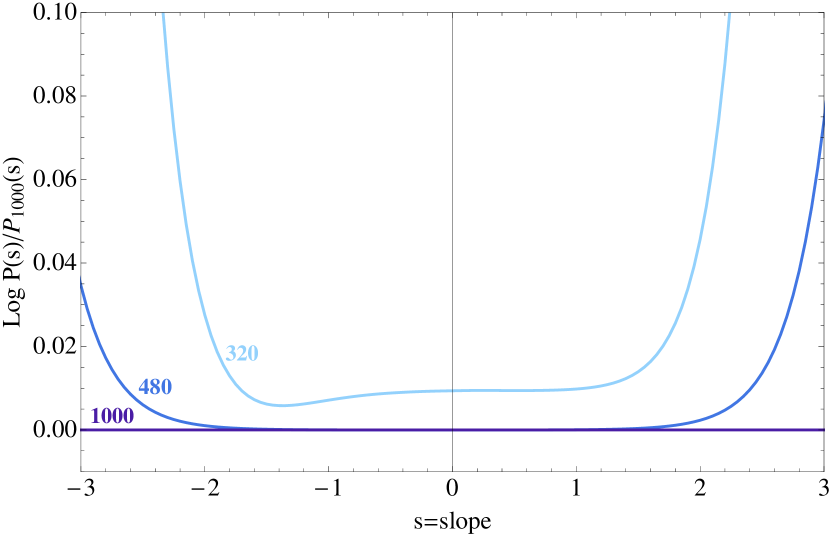
Figure 2: Dependence of the PDF of the slope on the number of points used in the numerical integration in (12). The reference PDF is computed using $1000^{2}$ points (dark blue) and is compared to the result of the numerical integration when using $320^{2}$ (blue) and $480^{2}$ (light blue) points.

In order to numerically compute equation (12), we simply choose the imaginary path $(\lambda_{1},\lambda_{2})=\hbox{i}(n_{1}\Delta\lambda,n_{2}\Delta\lambda)$ where $n_{1}$ and $n_{2}$ are (positive or negative) integers and the step $\Delta\lambda$ has been set to 0.15. The maximum value of $\lambda_{i}$ used here is 75 resulting into a discretisation of the integrand on $1000^{2}$ points. Fig. 1 compares the result of the numerical integration of equation (12) to simulations. The corresponding dark matter simulation (carried out with Gadget2 (Springel, 2005)) is characterized by the following $\Lambda$CDM cosmology: $\Omega_{\rm m}=0.265$, $\Omega_{\Lambda}=0.735$, $n=0.958$, $H_{0}=70$ km$\cdot s^{-1}\cdot$Mpc^-1 and $\sigma_{8}=0.8$, $\Omega_{b}=0.045$ within one standard deviation of WMAP7 results (Komatsu et al., 2011). The box size is 500 Mpc$/h$ sampled with $1024^{3}$ particles, the softening length 24 kpc$/h$. Initial conditions are generated using mpgrafic (Prunet et al., 2008). An Octree is built to count efficiently all particles within concentric spheres of radii between $R=10$ and $11{\rm Mpc}/h$. The center of these spheres is sampled regularly on a grid of $10\,{\rm Mpc}/h$ aside, leading to 117649 estimates of the density per snapshot. Note that the cells overlap for radii larger than $10\,{\rm Mpc}/h$.

The convergence of our numerical scheme is investigated by varying the number of points. Fig. 2 shows that the numerical integration of the slope PDF has reached 1% precision for the displayed range of slopes. Obviously, the integration is very precise for low values of the slope and requires a largest number of points for the large-slope tails.

3 Conditional distributions

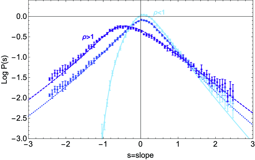
Figure 3: Density profiles in underdense (solid light blue), overdense (dashed purple) and all regions (dashed blue) for cells of radii $R_{1}=10$ Mpc/h and $R_{2}=11$ Mpc/h at redshift $z=0.97$. Predictions are successfully compared to measurements in simulations (points with error bars).

3.1 Slope in sub regions

Once the full 2-cell PDF is known, it is straightforward to derive predictions for density profiles restricted to underdense

$${\cal P}(\hat{s}|\hat{\rho}<1)=\frac{\int_{0}^{1}\hbox{d}\hat{\rho}\;\hat{\cal P}(\hat{\rho},\hat{s})}{\int_{-\infty}^{\infty}\hbox{d}\hat{s}\int_{0}^{1}\hbox{d}\hat{\rho}\;\hat{\cal P}(\hat{\rho},\hat{s})}\,,$$ (14)

and overdense regions

$${\cal P}(\hat{s}|\hat{\rho}>1)=\frac{\int_{1}^{\infty}\hbox{d}\hat{\rho}\;\hat{\cal P}(\hat{\rho},\hat{s})}{\int_{-\infty}^{\infty}\hbox{d}\hat{s}\int_{0}^{1}\hbox{d}\hat{\rho}\;\hat{\cal P}(\hat{\rho},\hat{s})}\,.$$ (15)

Fig. 3 displays these predicted density profiles in underdense and overdense regions compared to the measurements in our simulation. A very good agreement is found with some slight departures in the large slope tail of the distribution. As expected, the underdense slope PDF peaks towards positive slope, while the overdense PDF peaks towards negative slope. The constrained negative tails are more sensitive to the underlying constraint, providing improved leverage for measuring the underlying cosmological parameters.

3.2 Density in regions of given slope

Conversely, one can study the statistics of the density given constraints on the slope. For instance, the density PDF in regions of negative slope reads

$${\cal P}(\hat{\rho}|\hat{s}<0)=\frac{\int_{-\infty}^{0}\hbox{d}\hat{s}\;\hat{\cal P}(\hat{\rho},\hat{s})}{\int_{0}^{\infty}\hbox{d}\hat{\rho}\int_{-\infty}^{0}\hbox{d}\hat{s}\;\hat{\cal P}(\hat{\rho},\hat{s})}\,.$$ (16)

Fig. 4 displays the predicted density PDF in regions of positive or negative slope. As expected, the density is higher in regions of negative slope. An excellent agreement with simulations is found.

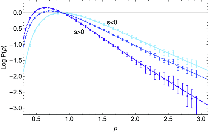
Figure 4: Density PDF in negative slope (solid light blue), positive slope (dashed purple) and all regions (dashed blue) for cells of radii $R_{1}=10$ Mpc/h and $R_{2}=11$ Mpc/h at redshift $z=0.97$. Predictions are successfully compared to measurements in simulations (points with error bars).

3.3 Redshift evolution

Fig. 5 displays the density profiles in underdense and overdense regions as measured in the simulation for a range of redshifts. This figure shows that the high density subset for moderately negative slopes is particularly sensitive to redshift evolution, which suggests that dark energy investigations should focus on such range of slopes and regions.

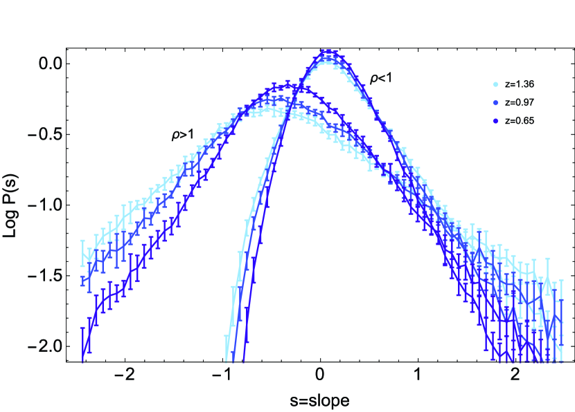
Figure 5: Same as Fig. 3 for a range of redshifts as labeled. Only the underdense ($\rho<1$) and the overdense ($\rho>1$) PDFs are shown.

4 Fiducial dark energy experiment

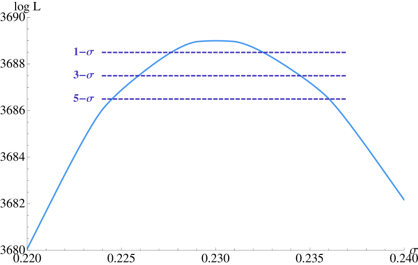
Figure 6: Log-likelihood for a fiducial experiment involving 10,000 concentric spheres of 10 and 11 Mpc$/h$ measured in our simulation. The model here only depends on the variance $\sigma$ ($\nu$ and $n$ are fixed). The contours at 1, 3 and 5 sigmas centered on the true value $0.23$ are displayed with dark blue dashed lines. The same experiment can be carried out when the three parameters vary.

Let us conduct the following fiducial experiment. Consider a set of 10,000 concentric spheres, and measure for each pair the slope and the density, $\{\hat{\rho}_{i},\hat{s}_{i}\}$. Recall that the cosmology is encoded in the parametrization of the spherical collapse on the one hand ($\nu$), and on the linear power-spectrum, $P^{\rm lin}_{k}$, (via the covariance matrix, $\Sigma_{ij}=\int P^{\rm lin}_{k}(k)W(R_{i}k)W(R_{j}k)d^{3}k/(2\pi)^{3}$ with $W(k)={3}\left(\sin(k)/k-\cos(k)\right)/{k^{2}}$) on the other hand. For scale invariant power spectra with power index $n$, given equation (8), we have a three parameter $(n,\nu,\sigma)$ set of models. For a parametrized PDF, $P_{n,\nu,\sigma}(\hat{\rho},\hat{s})$ given by equation (13), we can compute the log likelihood of the set as ${\cal L}(n,\nu,\sigma)=\sum_{i}\log P_{n,\nu,\sigma}(\hat{\rho}_{i},\hat{s}_{i})$. Fig. 6 displays the corresponding likelihood contours at one, three and five sigmas in the simple case in which only one parameter ($\sigma$ here) varies. This experiment mimics the precision expected from a survey of useful volume of about $(350h^{-1}\textrm{Mpc})^{3}$ which is found to be at the percent level. This work improves the findings of BPC which relies on a low-density approximation for the joint PDF.

5 Conclusion

Extending the analysis of BPC, predictions for the joint PDF of the density within two concentric spheres was straightforwardly implemented for a given cosmology as a function of redshift in the mildly non-linear regime. The agreement with measurements in simulation was shown on Figs. 1, 3 and 4 to be very good, including in the quasi-linear regime where standard perturbation theory normally fails. A fiducial dark energy experiment was implemented on counts derived from $\Lambda$CDM simulations.
Such statistics will prove useful in upcoming surveys as they allow us to probe differentially the slope of the density in regions of low or high density. It can serve as a statistical indicator to test gravity and dark energy models and/or probe key cosmological parameters in carefully chosen subsets of surveys. The theory of count-in-cells could be applied to 2D cosmic shear maps so as to predict the statistics of projected density profiles. Velocity profiles and combined probes involving the density and velocity fields should also be within reach of this formalism.

Acknowledgements: This work is partially supported by the grants ANR-12-BS05-0002 and ANR-13-BS05-0005 of the French Agence Nationale de la Recherche. The simulations were run on the Horizon cluster. We acknowledge support from S. Rouberol for running the cluster for us.

References

- Balian & Schaeffer (1989) Balian R., Schaeffer R., 1989, Astr. & Astrophys. , 220, 1
- Bernardeau (1992) Bernardeau F., 1992, Astrophys. J. Letter, 390, L61
- Bernardeau (1994) Bernardeau F., 1994, Astr. & Astrophys. , 291, 697
- Bernardeau et al. (2014) Bernardeau F., Pichon C., Codis S., 2014, Phys. Rev. D , 90, 103519
- Juszkiewicz et al. (1993) Juszkiewicz R., Bouchet F. R., Colombi S., 1993, Astrophys. J. Letter, 412, L9
- Komatsu et al. (2011) Komatsu E., Smith K. M., Dunkley J., Bennett C. L., Gold B., Hinshaw G., Jarosik N., Larson D., et al. 2011, Astrophys. J. Suppl. Ser. , 192, 18
- Laureijs et al. (2011) Laureijs R., Amiaux J., Arduini S., Auguères J. ., Brinchmann J., Cole R., Cropper M., Dabin C., Duvet L., Ealet A., et al. 2011, ArXiv e-prints
- Prunet et al. (2008) Prunet S., Pichon C., Aubert D., Pogosyan D., Teyssier R., Gottloeber S., 2008, Astrophys. J. Suppl. Ser. , 178, 179
- Scoccimarro et al. (1998) Scoccimarro R., Colombi S., Fry J. N., Frieman J. A., Hivon E., Melott A., 1998, Astrophys. J. , 496, 586
- Springel (2005) Springel V., 2005, Mon. Not. R. Astr. Soc. , 364, 1105
- Valageas (2002) Valageas P., 2002, Astr. & Astrophys. , 382, 412