A Proximal Approach for Sparse Multiclass SVM

Abstract

Sparsity-inducing penalties are useful tools to design multiclass support vector machines (SVMs). In this paper, we propose a convex optimization approach for efficiently and exactly solving the multiclass SVM learning problem involving a sparse regularization and the multiclass hinge loss formulated by [1]. We provide two algorithms: the first one dealing with the hinge loss as a penalty term, and the other one addressing the case when the hinge loss is enforced through a constraint. The related convex optimization problems can be efficiently solved thanks to the flexibility offered by recent primal-dual proximal algorithms and epigraphical splitting techniques. Experiments carried out on several datasets demonstrate the interest of considering the exact expression of the hinge loss rather than a smooth approximation. The efficiency of the proposed algorithms w.r.t. several state-of-the-art methods is also assessed through comparisons of execution times.

1 Introduction

Support vector machines (SVMs) have gained much popularity in solving large-scale classification problems. As a matter of fact, many applications considered in the literature deal with a large amount of training data or a huge (even infinite) number of classes [2, 3, 4, 5, 6]. Consequently, the major difficulty encountered in this kind of applications stems from the computational cost. The SVM learning problem is classically solved by using standard Lagrangian duality techniques [7, 1]. This approach brings in several advantages, such as the kernel trick [8], or the possibility to break the problem down into a sequence of smaller ones [9, 10]. Some works also proposed to approximate the dual problem using cutting plane approaches, in order to address scenarios with thousands or even an infinite number of classes [3, 6].

In some applications, however, only a small number of training data is available. This is undoubtedly true in medical contexts, where the goal is to classify a patient as being “healthy”, “contaminated”, or “infected”, but the verified cases of infected patients might be just a few. In such applications, the lack of training data may lead to the so-called overfitting problem, eventually leading to a prediction which is too strongly tailored to the particularities of the training set and poorly generalizes to new data.

A common solution to prevent overfitting consists of introducing a sparsity-inducing regularization in order to perform an implicit feature selection that gets rid of irrelevant or noisy features. In this respect, the $\boldsymbol{\ell}_{1}$-norm and, more generally, the $\boldsymbol{\ell}_{1,p}$-norm regularization have attracted much attention over the past decade [11, 12, 13, 14, 15, 16, 17, 18]. However, when a sparse regularization is introduced, the dual approach does no longer yield a simple formulation. Therefore, SVMs with sparse regularization lead to a nonsmooth convex optimization problem which is challenging. The main objective of this paper is to exactly and efficiently solve the multiclass SVM learning problem for convex regularizations. To this end, we propose two algorithms based on a primal-dual proximal method [19, 20] and a novel epigraphical splitting technique [21]. In addition to more detailed theoretical developments, this paper extends our preliminary work [22] by providing a new algorithm, and a larger number of experiments including comparisons with state-of-the-art methods for different types of database.

1.1 Related work

The use of sparse regularization in SVMs was firstly proposed in the context of binary classification. The idea traces back to the work by [23], who demonstrated that the $\boldsymbol{\ell}_{1}$-norm regularization can effectively perform “feature selection” by shrinking small coefficients to zero. Other forms of regularization have also been studied, such as the $\boldsymbol{\ell}_{0}$-norm [24], the $\boldsymbol{\ell}_{p}$-norm with $p>0$ [25], the $\boldsymbol{\ell}_{\infty}$-norm [26], and the combination of $\boldsymbol{\ell}_{0}$-$\boldsymbol{\ell}_{1}$ norms [27] or $\boldsymbol{\ell}_{1}$-$\boldsymbol{\ell}_{2}$ norms [28]. A different solution was proposed by [29], who reformulated the SVM learning problem by using an indicator vector (its components being either equal to 0 or 1) to model the active features, and solved the resulting combinatorial problem by convex relaxation using a cutting-plane algorithm. More recently, [30] proposed an accelerated algorithm for $\boldsymbol{\ell}_{1}$-regularized SVMs involving the square hinge loss. They also proposed a procedure for handling nonconvex regularization (using the reweighted $\boldsymbol{\ell}_{1}$-minimization scheme by [31]), showing that nonconvex penalties lead to similar prediction quality while using less features than convex ones.

Binary SVMs can be turned into multiclass classifiers by a variety of strategies, such as the one-vs-all approach [7, 32]. While these techniques provide a simple and powerful framework, they cannot capture the correlations between different classes, since they break a multiclass problem into multiple independent binary problems. [1] therefore proposed a direct formulation of multiclass SVMs by generalizing the notion of margins used in the binary case. A natural idea thus consists of equipping muticlass SVMs with sparse regularization. A simple example is the $\boldsymbol{\ell}_{1}$-regularized multiclass SVM, which can be addressed by linear programming techniques [33]. In multiclass problems however, feature selection becomes more complex than in the binary case, since multiple discriminating functions need to be estimated, each one with its own set of important features. For this reason, mixed-norm regularization has recently attracted much interest due to its ability to impose group sparsity [34, 35, 12, 36]. In the context of multiclass SVMs, [37] proposed to deal with the $\boldsymbol{\ell}_{1,\infty}$-norm regularization by reformulating the SVM learning problem in terms of linear programming. However, they validated their method on small-size problems, indicating that the linear reformulation may be inefficient for larger-size ones. More recently, [38] proposed an algorithm to handle $\boldsymbol{\ell}_{1,2}$-regularized SVMs involving a smooth loss function. While their method is efficient and can handle other convex regularizations, it does not solve rigorously the multiclass SVM learning problem, possibly leading to performance limitations.

1.2 Contributions

The algorithmic solutions proposed in the literature to deal with sparse multiclass SVMs are either cutting-plane methods [29], proximal algorithms [30, 38], or linear programming techniques [33, 37]. However, both cutting-plane methods and proximal algorithms have been employed to find an approximate solution, while linear programming techniques may not scale well to large datasets. In this paper, we propose a novel approach based on proximal tools and recent epigraphical splitting techniques [21], which allow us to exactly solve the sparse multiclass SVM learning problem through an efficient primal-dual proximal method [19, 20].

1.3 Outline

The paper is organized as follows. In Section 2, we formulate the multiclass SVM problem with sparse regularization, in Section 3 we provide the proximal tools needed to solve the proposed problem, and in Section 4 we evaluate our approach on three standard datasets and compare it to the methods proposed by [38], [30], [37], and [11].

1.4 Notation

$\Gamma_{0}(\mathbb{R}^{X})$ denotes the set of proper, lower semicontinuous, convex functions from the Euclidean space $\mathbb{R}^{X}$ to $\left]-\infty,+\infty\right]$. The epigraph of $\psi\in\Gamma_{0}(\mathbb{R}^{X})$ is the nonempty closed convex subset of $\mathbb{R}^{X}\times\mathbb{R}$ defined as $\operatorname{epi}\psi=\big{\{}{(y,\zeta)\in\mathbb{R}^{X}\times\mathbb{R}}~{}\big{|}~{}{\psi(y)\leq\zeta}\big{\}}$. For every $x\in\mathbb{R}^{X}$, the subdifferential of $\psi$ at $x$ is $\partial\psi(x)=\big{\{}{u\in\mathbb{R}^{X}}~{}\big{|}~{}{(\forall y\in\mathbb{R}^{X})\;{\left\langle{{y-x}\mid{u}}\right\rangle}+\psi(x)\leq\psi(y)}\big{\}}$. Let $C$ be a nonempty closed convex subset of $\mathbb{R}^{X}$, then $\iota_{C}$ is the indicator function of $C$, equal to $0$ on $C$ and ${+\infty}$ otherwise.

2 Sparse Multiclass SVM

A multiclass classifier can be modeled as a function $d\colon\mathbb{R}^{N}\to\{1,\dots,K\}$ that predicts the class $k\in\{1,\dots,K\}$ associated to a given observation $u\in\mathbb{R}^{N}$ (e.g. a signal, an image or a graph). This predictor relies on $K$ different discriminating functions $D_{k}\colon\mathbb{R}^{N}\mapsto\mathbb{R}$ which, for every $k\in\{1,\dots,K\}$, measure the likelihood that an observation belongs to the class $k$. Consequently, the predictor selects the class that best matches an observation, i.e.

$$d(u)\in\operatorname*{argmax\;}_{k\in\{1,\dots,K\}}D_{k}(u).$$

In supervised learning, the discriminating functions are built from a set of $L$ input-output pairs

$$S=\big{\{}(u_{\ell},z_{\ell})\in\mathbb{R}^{N}\times\{1,\dots,K\}\;|\;\ell=\{1,\dots,L\}\big{\}},$$

and they are assumed to be linear in some feature representation of inputs [39]. The latter assumption leads to the following form of the discriminating functions:

$$D_{k}(u)=\phi(u)^{\top}x^{(k)}+b^{(k)},$$ (1)

where $\phi\colon\mathbb{R}^{N}\mapsto\mathbb{R}^{M}$ denotes a mapping from the input space onto an arbitrary feature space, and $(x^{(k)},b^{(k)})_{1\leq k\leq K}$ denote the parameters to be estimated. For convenience, we concatenate the latter ones into a single vector ${\rm x}\in\mathbb{R}^{(M+1)K}$

$${\rm x}=\left[\begin{aligned} &x^{(1)}\\ &b^{(1)}\\ &\;\;\,\vdots\\ &x^{(K)}\\ &b^{(K)}\\ \end{aligned}\right]\begin{aligned} &\left.\vphantom{\begin{aligned} x^{(1)}\\ b^{(1)}\end{aligned}}\right\}{\rm x}^{(1)}\\ &\vphantom{\vdots}\\ &\left.\vphantom{\begin{aligned} x^{(K)}\\ b^{(K)}\end{aligned}}\right\}{\rm x}^{(K)}\end{aligned}$$

and we define the function $\varphi\colon\mathbb{R}^{N}\mapsto\mathbb{R}^{M+1}$ as

$$\varphi(u)=\left[\phi(u)^{\top}\;\;1\right]^{\top},$$

so that (1) can be shortened to $D_{k}(u)=\varphi(u)^{\top}{\rm x}^{(k)}$.

2.1 Background

The objective of learning consists of finding the vector ${\rm x}$ such that, for every $\ell\in\{1,\dots,L\}$, the input-output pair $(u_{\ell},z_{\ell})\in S$ is correctly predicted by the classifier, i.e.,

$$z_{\ell}=\operatorname*{argmax\;}_{k\in\{1,\dots,K\}}\varphi(u_{\ell})^{\top}{\rm x}^{(k)}.$$

By the definition of $\operatorname{argmax}$, the above equality holds if

$$(\forall\ell\in\{1,...,L\})\quad\max_{k\neq z_{\ell}}\;\varphi(u_{\ell})^{\top}({\rm x}^{(k)}-{\rm x}^{(z_{\ell})})<0,$$

or, equivalently,

$$(\forall\ell\in\{1,...,L\})\quad\max_{k\neq z_{\ell}}\;\varphi(u_{\ell})^{\top}({\rm x}^{(k)}-{\rm x}^{(z_{\ell})})\leq-\mu_{\ell},$$ (2)

where, for every $\ell\in\{1,\dots,L\}$, $\mu_{\ell}$ is a positive scalar. Unfortunately, this constraint has no practical interest for learning purposes, as it becomes infeasible when the training set is not fully separable. Multiclass SVMs overcome this issue by introducing the notion of soft margins, which consists of adding a vector of slack variables $\xi=(\xi^{(\ell)})_{1\leq\ell\leq L}$ into (2):

$$\left\{\begin{aligned} \!\!&(\forall\ell\in\{1,...,L\})\;\max_{k\neq z_{\ell}}\;\varphi(u_{\ell})^{\top}({\rm x}^{(k)}-{\rm x}^{(z_{\ell})})\leq\xi^{(\ell)}-\mu_{\ell},\\ \!\!&(\forall\ell\in\{1,...,L\})\;\xi^{(\ell)}\geq 0,\end{aligned}\right.$$ (3)

The multiclass SVM learning problem is thus obtained by adding a quadratic regularization [1], yielding

$$\underset{\begin{subarray}{c}{({\rm x},\xi)\in\mathbb{R}^{(M+1)K}\times\mathbb{R}^{L}}\end{subarray}}{\operatorname{minimize}}\;\;\;\sum_{k=1}^{K}\|x^{(k)}\|_{2}^{2}+\lambda\sum_{\ell=1}^{L}\xi^{(\ell)}\quad\operatorname{s.t.}\\ \left\{\begin{aligned} \!\!&(\forall\ell\in\{1,...,L\})\quad\max_{k\neq z_{\ell}}\;\varphi(u_{\ell})^{\top}({\rm x}^{(k)}-{\rm x}^{(z_{\ell})})\leq\xi^{(\ell)}-\mu_{\ell},\\ \!\!&(\forall\ell\in\{1,...,L\})\quad\xi^{(\ell)}\geq 0,\end{aligned}\right.$$ (4)

where $\lambda\in\left]0,+\infty\right[$. Note that the linear penalty on the slack variables allows us to minimize the violation of constraint (2). By using standard convex analysis [40], the above problem can be equivalently rewritten without slack variables as

$$\operatorname*{minimize}_{{\rm x}\in\mathbb{R}^{(M+1)K}}\;\sum_{k=1}^{K}\|x^{(k)}\|_{2}^{2}+\lambda\sum_{\ell=1}^{L}\max\big{\{}0,\mu_{\ell}+\max_{k\neq z_{\ell}}\;\varphi(u_{\ell})^{\top}({\rm x}^{(k)}-{\rm x}^{(z_{\ell})})\big{\}}.$$ (5)

Hereabove, the second term is called hinge loss when $\mu_{\ell}\equiv 1$.

2.2 Proposed approach

We extend Problem (5) by replacing the squared $\boldsymbol{\ell}_{2}$-norm regularization with a generic function $g\in\Gamma_{0}(\mathbb{R}^{(M+1)K})$. Moreover, we rewrite the hinge loss in an equivalent form by introducing, for every $\ell\in\{1,\dots,L\}$, the linear operator $T_{\ell}\colon\mathbb{R}^{(M+1)K}\mapsto\mathbb{R}^{K}$ defined as

$$\big{(}\forall{\rm x}\in\mathbb{R}^{(M+1)K}\big{)}\quad T_{\ell}\,{\rm x}=\big{[}\,\varphi(u_{\ell})^{\top}({\rm x}^{(k)}-{\rm x}^{(z_{\ell})})\,\big{]}_{1\leq k\leq K},$$

the vector $r_{\ell}=(r_{\ell}^{(k)})_{1\leq k\leq K}\in\mathbb{R}^{K}$ defined as

$$(\forall k\in\{1,\dots,K\})\qquad r_{\ell}^{(k)}=\begin{cases}0,&\quad\textrm{if $k=z_{\ell}$},\\ \mu_{\ell},&\quad\textrm{otherwise},\end{cases}$$

and the function $h_{\ell}\colon\mathbb{R}^{K}\mapsto\mathbb{R}$ defined, for every $y^{(\ell)}=(y^{(\ell,k)})_{1\leq k\leq K}\in\mathbb{R}^{K}$, as

$$h_{\ell}(y^{(\ell)})=\max_{1\leq k\leq K}y^{(\ell,k)}+r_{\ell}^{(k)},$$ (6)

so that the following holds

$$h_{\ell}(T_{\ell}{\rm x})=\max\big{\{}0,\mu_{\ell}+\max_{k\neq z_{\ell}}\;\varphi(u_{\ell})^{\top}({\rm x}^{(k)}-{\rm x}^{(z_{\ell})})\big{\}}.$$

We aim at solving the following convex optimization problems:

• regularized formulation

  $$\underset{\begin{subarray}{c}{{\rm x}\in\mathbb{R}^{(M+1)K}}\end{subarray}}{\operatorname{minimize}}\;\;\;g({\rm x})+\lambda\sum_{\ell=1}^{L}h_{\ell}(T_{\ell}\,{\rm x}),$$ (7)

• constrained formulation

  $$\underset{\begin{subarray}{c}{{\rm x}\in\mathbb{R}^{(M+1)K}}\end{subarray}}{\operatorname{minimize}}\;\;\;g({\rm x})\quad\operatorname{s.t.}\quad\sum_{\ell=1}^{L}h_{\ell}(T_{\ell}\,{\rm x})\leq\eta,$$ (8)

where $\lambda$ and $\eta$ are positive constants. Note that, by Lagrangian duality, the above formulations are equivalent for some specific values of $\eta$ and $\lambda$. The interest of considering the constrained formulation lies in the fact that $\eta$ may be easier to set, since it is directly related to the properties of the training data.

As mentioned in the introduction, the regularization term $g$ is chosen so as to promote some form of sparsity. A popular example is the $\boldsymbol{\ell}_{1}$-norm, as it ensures that the solution will have a number of coefficients exactly equal to zero, depending on the strength of the regularization [15]. Another example is given by the mixed $\boldsymbol{\ell}_{1,p}$-norm. For every ${\rm x}\in\mathbb{R}^{(M+1)K}$, let us assume that, for each $k\in\{1,\dots,K\}$, the vector ${\rm x}^{(k)}\in\mathbb{R}^{M+1}$ is block-decomposed as follows:

$${\rm x}^{(k)}=\Big{[}\underbrace{\left(x^{(k,1)}\right)^{\top}}_{\text{size}\,M_{1}}\quad\dots\quad\underbrace{\left(x^{(k,B)}\right)^{\top}}_{\text{size}\,M_{B}}\quad b^{(k)}\Big{]}^{\top},$$

with $M_{1}+\dots+M_{B}=M$. We define the $\boldsymbol{\ell}_{1,p}$-norm as

$$g({\rm x})=\sum_{k=1}^{K}\sum_{b=1}^{B}\|x^{(k,b)}\|_{p}.$$

The mixed-norm regularization is known to induce block-sparsity: the solution is partitioned into groups and the components of each group are ideally either all zeros or all non-zeros. In this context, the exponent values $p=2$ or $p=+\infty$ are the most popular choices. In particular, the $\boldsymbol{\ell}_{1,\infty}$-norm tends to favor solutions with few nonzero groups having components of similar magnitude.

3 Optimization method

The resolution of Problems (7) and (8) requires an efficient algorithm for dealing with nonsmooth functions and hard constraints. In the convex optimization literature, proximal algorithms constitute one of the most efficient approaches to deal with nonsmooth problems [41, 42, 15, 43, 44]. The key tool in these methods is the proximity operator [45], defined for a function $\psi\in\Gamma_{0}({\mathcal{H}})$ as

$$(\forall u\in{\mathcal{H}})\qquad\operatorname{prox}_{\psi}(u)=\operatorname*{argmin}_{v\in{\mathcal{H}}}\;\frac{1}{2}\|v-u\|^{2}+\psi(v).$$

The proximity operator can be interpreted as a sort of subgradient step for the function $\psi$, as $p=\operatorname{prox}_{\psi}(y)$ is uniquely defined through the inclusion $y-p\in\partial\psi(p)$. In addition, it reverts to the projection onto a closed convex set $C\subset{\mathcal{H}}$ in the case when $\psi=\iota_{C}$, in the sense that

$$(\forall u\in{\mathcal{H}})\qquad\operatorname{prox}_{\iota_{C}}(u)=P_{C}(u)=\operatorname*{argmin}_{v\in C}\;\frac{1}{2}\|v-u\|^{2}.$$ (9)

Proximal algorithms work by iterating a sequence of steps in which the proximity operators of the functions involved in the minimization are evaluated at each iteration. An efficient computation of these operators is thus essential to design fast algorithms for solving Problems (7)-(8). In the next sections, we will present two different approaches based on a Forward-Backward based Primal-Dual method (FBPD) [19, 20, 46, 47, 48], which we have selected among the large panel of proximal algorithms for its simplicity to deal with large-size linear operators.

3.1 Regularized formulation

Problem (7) fits nicely into the framework provided by FBPD algorithm, since the proximity operators of both $g$ and $(h_{\ell})_{1\leq\ell\leq L}$ can be efficiently computed. Indeed, $\operatorname{prox}_{g}$ has a closed form for several norms and mixed norms [43, 41], while $(\operatorname{prox}_{h_{\ell}})_{1\leq\ell\leq L}$ can be computed through the projection onto the standard simplex, as described in Proposition 3.1. The projection onto the simplex can be efficiently computed with the method proposed by [49].

Proposition 3.1.

For every $\ell\in\{1,\ldots,L\}$,

$$(\forall{y}^{(\ell)}\in\mathbb{R}^{K})\quad\operatorname{prox}_{\lambda h_{\ell}}\big{(}y^{(\ell)}\big{)}=y^{(\ell)}-P_{S_{\lambda}}\big{(}y^{(\ell)}+r_{\ell}\big{)},$$ (10)

with

$$S_{\lambda}=\big{\{}{u=\big{(}u^{(k)}\big{)}_{1\leq k\leq K}\in[0,+\infty[^{K}}~{}\big{|}~{}{\sum_{k=1}^{K}u^{(k)}=\lambda}\big{\}}.$$

Proof.

Note that $u\in\mathbb{R}^{K}\!\mapsto\!\lambda\max_{1\leq k\leq K}u^{(k)}$ is the support function of $S_{\lambda}$, defined as $(\forall u\in\mathbb{R}^{K})$ $\sigma_{S_{\lambda}}(u)=\sup_{v\in S_{\lambda}}v^{\top}u$. Hence, for every ${y}^{(\ell)}\in\mathbb{R}^{K}$, $\lambda h_{\ell}({y}^{(\ell)})=\sigma_{S_{\lambda}}({y}^{(\ell)}+r_{\ell})$ and

$$\operatorname{prox}_{\lambda h_{\ell}}\big{(}y^{(\ell)}\big{)}=\operatorname{prox}_{\sigma_{S_{\lambda}}}(y^{(\ell)}+r_{\ell})-r_{\ell},$$

Since $\sigma_{S_{\lambda}}$ is the conjugate function of $\iota_{S_{\lambda}}$, (10) is deduced by applying Moreau’s decomposition formula [50, Theorem 14.3(ii)] and (9). ∎

The iterations associated with Problem (7) are summarized in Algorithm 1, where the sequence $({\rm x}^{[i]})_{i\in\mathbb{N}}$ is guaranteed to converge to a solution to Problem (7), provided that such a solution exists [19, 20]. In Algorithm 1, we use the notation

$$T=[T_{1}^{\top}\;\dots\;T_{L}^{\top}]^{\top},\qquad r=[r_{1}^{\top}\;\dots\;r_{L}^{\top}]^{\top}.$$

Remark 3.2.

Algorithm 1 allows us to solve Problem (7) together with its (Fenchel-Rockafellar) dual formulation

$$\underset{\begin{subarray}{c}{y\in\mathbb{R}^{LK}}\end{subarray}}{\operatorname{minimize}}\;\;\;g^{*}(-T^{\top}y)-\sum_{\ell=1}^{L}r_{\ell}^{\top}y^{(\ell)}\quad\operatorname{s.t.}\quad y\in(S_{\lambda})^{L},$$ (11)

where $g^{*}$ is the convex conjugate of $g$. In the case when $g=(1/2)\|\cdot\|^{2}_{2}$, the primal and dual solutions are linked by ${\rm x}=-T^{\top}y$, and thus Problem (11) reduces to the (Lagrangian) dual formulation of Problem (4) used in standard SVMs [1].

Algorithm 1 FBPD for solving Problem (7)

Initialization

$$\!\!\!\!\!\!\!\!\!\!\!\!\!\!\!\!\!\!\!\!\!\!\!\left\lfloor\begin{aligned} &\textrm{choose ${{\rm x}^{[0]}}\in\mathbb{R}^{(M+1)K}$}\\ &\textrm{choose ${y^{[0]}}\in\mathbb{R}^{LK}$}\\ &\textrm{set $\tau>0$ and $\sigma>0$ such that $\tau\sigma\|T\|^{2}\leq 1$.}\\ \end{aligned}\right.\\$$

For  i = 0, 1, …

$$\!\!\!\!\!\!\!\!\!\!\!\!\!\!\!\!\!\!\!\!\!\!\!\!\!\!\!\!\!\!\!\!\!\!\!\!\!\!\!\!\!\!\!\!\!\!\!\left\lfloor\begin{aligned} &{\rm x}^{[i+1]}=\operatorname{prox}_{\tau g}\big{(}{\rm x}^{[i]}-\tau\,T^{\top}y^{[i]}\big{)}\\ &\widehat{y}^{[i+1]}=y^{[i]}+\sigma T\big{(}2{\rm x}^{[i+1]}-{\rm x}^{[i]}\big{)}\\ &y^{[i+1]}=P_{(S_{\lambda})^{L}}\left(\widehat{y}^{[i+1]}+\sigma\,r\right).\end{aligned}\right.$$

3.2 Constrained formulation

Problem (8) presents a more challenging computational issue, as the projection onto the hinge-loss constraint set cannot be evaluated in closed form, and it would require to solve a constrained quadratic problem at each iteration. In order to manage this constraint, we propose to introduce a vector of auxiliary variables $\zeta=\big{(}\zeta^{(\ell)}\big{)}_{1\leq\ell\leq L}$ in the minimization process, so that Problem (8) can be equivalently rewritten as

$$\underset{\begin{subarray}{c}{({\rm x},\zeta)\in\mathbb{R}^{(M+1)K}\times\mathbb{R}^{L}}\end{subarray}}{\operatorname{minimize}}\;\;\;g({\rm x})\quad\operatorname{s.t.}\quad\left\{\begin{aligned} &\sum_{\ell=1}^{L}\zeta^{(\ell)}\leq\eta,\\ &(\forall\ell\in\{1,\ldots,L\})&&h_{\ell}(T_{\ell}\,{\rm x})\leq\zeta^{(\ell)}.\end{aligned}\right.$$ (12)

Interestingly, our approach is conceptually similar to adding the slack variables in (3), even though our reformulation specifically aims at simplifying the way of solving the problem. Indeed, a possible interpretation of Problem (12) is the following:

$$\underset{\begin{subarray}{c}{({\rm x},\zeta)\in\mathbb{R}^{(M+1)K}\times\mathbb{R}^{L}}\end{subarray}}{\operatorname{minimize}}\;\;g({\rm x})\quad\operatorname{s.t.}\quad\begin{cases}(T{\rm x},&\!\!\!\!\zeta)\in E,\\ &\!\!\!\!\zeta\hphantom{)}\in V_{\eta},\end{cases}$$ (13)

where $E$ denotes the collection of epigraphs of $h_{1},\dots,h_{L}$

$$E=\big{\{}{(y,\zeta)\in\mathbb{R}^{LK}\times\mathbb{R}^{L}}~{}\big{|}~{}{(\forall\ell\in\{1,\dots,L\})\quad(y^{(\ell)},\zeta^{(\ell)})\in\operatorname{epi}h_{\ell}}\big{\}},$$

and $V_{\eta}$ denotes a closed half-space

$$V_{\eta}=\big{\{}{\zeta\in\mathbb{R}^{L}}~{}\big{|}~{}{\sum_{\ell=1}^{L}\zeta^{(\ell)}\leq\eta}\big{\}}.$$

The iterations related to Problem (13) are listed in Algorithm 2, where the sequence $({\rm x}^{[i]},\zeta^{[i]})_{i\in\mathbb{N}}$ is guaranteed to converge to a solution to (13), provided that such a solution exists [19, 20].

Algorithm 2 FBPD for solving Problem (8)

Initialization

$$\left\lfloor\begin{aligned} &\textrm{choose $({\rm x}^{[0]},\zeta^{[0]})\in\mathbb{R}^{(M+1)K}\times\mathbb{R}^{L}$}\\ &\textrm{choose $(y^{[0]},\xi^{[0]})\in\mathbb{R}^{L(K-1)}\times\mathbb{R}^{L}$}\\ &\textrm{set $\tau>0$ and $\sigma>0$ such that $\tau\sigma\max\{\|T\|^{2},1\}\leq 1$}.\\ \end{aligned}\right.\\$$

For  i = 0, 1, …

$$\!\!\!\!\!\!\!\!\!\!\!\!\!\!\!\!\!\!\!\!\!\!\!\!\!\!\!\!\!\!\!\!\!\!\!\!\!\!\!\!\!\!\!\!\!\!\!\left\lfloor\begin{aligned} &{\rm x}^{[i+1]}=\operatorname{prox}_{\tau g}\big{(}{\rm x}^{[i]}-\tau\,T^{\top}y^{[i]}\big{)}\\ &\zeta^{[i+1]}=P_{V_{\eta}}\big{(}\zeta^{[i]}-\tau\,\xi^{[i]}\big{)}\\ &\widehat{y}^{[i]}=y^{[i]}+\sigma T\big{(}2{\rm x}^{[i+1]}-{\rm x}^{[i]}\big{)}\\ &\widehat{\xi}^{[i]}=\xi^{[i]}+\sigma\big{(}2\zeta^{[i+1]}-\zeta^{[i]}\big{)}\\ &\big{(}\widetilde{y}^{[i]},\widetilde{\xi}^{[i]}\big{)}=P_{E}\big{(}\widehat{y}^{[i]}/\sigma,\widehat{\xi}^{[i]}/\sigma\big{)}\\ &y^{[i+1]}=\widehat{y}^{[i]}-\sigma\widetilde{y}^{[i]}\\ &\xi^{[i+1]}=\widehat{\xi}^{[i]}-\sigma\widetilde{\xi}^{[i]}.\end{aligned}\right.$$

The advantage of our approach lies in the fact that the projections onto $E$ and $V_{\eta}$ employed in Algorithm 2 have closed form expressions. Indeed, the projection onto $V_{\eta}$ is straightforward [43, Section 6.2.3], while the projection onto $E$ can be block-decomposed as

$$P_{E}(y,\zeta)=\Big{(}P_{\operatorname{epi}h_{\ell}}(y^{(\ell)},\zeta^{(\ell)})\Big{)}_{1\leq\ell\leq L}$$ (14)

where a closed-form expression of $P_{\operatorname{epi}h_{\ell}}$ with $\ell\in\{1,\ldots,L\}$ is given in Proposition 3.3. The proof of this new result follows the same line as the proof by [21, Proposition 5], where we derived the epigraphical projection associated to the $\ell_{\infty}$-norm.

The decomposition in (14) yields two potential benefits. Firstly, the projection $P_{\operatorname{epi}h_{\ell}}$ is computed onto the lower-dimensional convex subset $\operatorname{epi}h_{\ell}$ of $\mathbb{R}^{K}\times\mathbb{R}$, whose dimensionality is only fixed by the number $K$ of classes. Secondly, these projections can be computed in parallel, since they are defined over disjoint blocks whose number is given by the cardinality $L$ of the training set (we refer to [51] for an example of parallel implementation on GP-GPUs).

Proposition 3.3.

For every $\ell\in\{1,\ldots,L\}$, let $h_{\ell}$ be the function defined in (6) and, for every $({y}^{(\ell)},\zeta^{(\ell)})\in\mathbb{R}^{K}\times\mathbb{R}$, let $\big{(}\nu^{(\ell,k)}\big{)}_{1\leq k\leq K}$ be the sequence $\big{(}y^{(\ell,k)}+r^{(k)}_{\ell}\big{)}_{1\leq k\leq K}$ sorted in ascending order, and set $\nu^{(\ell,0)}=-\infty$ and $\nu^{(\ell,K+1)}={+\infty}$. Then, $P_{\operatorname{epi}h_{\ell}}({y}^{(\ell)},\zeta^{(\ell)})=({p}^{(\ell)},\theta^{(\ell)})$ with

$$p^{(\ell)}=\Big{[}\,\min\{y^{(\ell,k)},\theta^{(\ell)}-r^{(k)}_{\ell}\}\,\Big{]}_{1\leq k\leq K}$$

and

$$\theta^{(\ell)}=\frac{1}{K-\overline{k}^{(\ell)}+2}\left(\zeta^{(\ell)}+\sum_{k=\overline{k}^{(\ell)}}^{K}\nu^{(\ell,k)}\right),$$ (15)

where $\overline{k}^{(\ell)}$ is the unique integer in $\{1,\ldots,K+1\}$ such that

$$\nu^{(\ell,\overline{k}^{(\ell)}-1)}<\theta^{(\ell)}\leq\nu^{(\ell,\overline{k}^{(\ell)})},$$ (16)

with the convention $\sum_{k=K+1}^{K}\cdot=0$.

Proof.

For every $(y^{(\ell)},\zeta^{(\ell)})\in\mathbb{R}^{K}\times\mathbb{R}$, $P_{\operatorname{epi}h_{\ell}}(y^{(\ell)},\zeta^{(\ell)})$ denotes the unique solution to

$$\min_{(p^{(\ell)},\theta^{(\ell)})\in\operatorname{epi}h_{\ell}}\|p^{(\ell)}-y^{(\ell)}\|^{2}+(\theta^{(\ell)}-\zeta^{(\ell)})^{2},$$

which is equivalent to find the minimizer of

$$\min_{\theta^{(\ell)}\in\mathbb{R}}\;\Big{\{}(\theta^{(\ell)}-\zeta^{(\ell)})^{2}+\!\!\!\!\min_{\begin{subarray}{c}\;\;\;{p}^{(\ell,1)}\leq\theta^{(\ell)}-r_{\ell}^{(1)}\\ \vdots\\ {p}^{(\ell,K)}\leq\theta^{(\ell)}-r_{\ell}^{(K)}\end{subarray}}\|{p}^{(\ell)}-{y}^{(\ell)}\|^{2}\Big{\}}.$$ (17)

For every $\theta^{(\ell)}\in\mathbb{R}$, the inner minimization is achieved when $p^{(\ell,k)}\!=\!\min\{y^{(\ell,k)},\theta^{(\ell)}-r^{(k)}_{\ell}\}$ for each $k\in\{1,\dots,K\}$, reducing (17) to

$$\underset{\theta^{(\ell)}\in\mathbb{R}}{\operatorname{min}}\;\Big{\{}(\theta^{(\ell)}-\zeta^{(\ell)})^{2}+\sum_{k=1}^{K}(\max\{{y}^{(\ell,k)}+r^{(k)}_{\ell}-\theta^{(\ell)},0\})^{2}\Big{\}},$$

which achieves its minimum when $\theta^{(\ell)}=\operatorname{prox}_{\varphi_{\ell}}(\zeta^{(\ell)})$, with

$$(\forall v\in\mathbb{R})\qquad\varphi_{\ell}(v)=\frac{1}{2}\sum_{k=1}^{K}(\max\{{y}^{(\ell,k)}+r^{(k)}_{\ell}-v,0\})^{2}.$$ (18)

The closed-form expression of this proximity operator, as well as the projection onto $\operatorname{epi}h_{\ell}$, are derived in the following. In order to prove (15), we need to compute the proximity operator of $\varphi_{\ell}$ defined in (18). Such a function belongs to $\Gamma_{0}(\mathbb{R})$ since, for each $k\!\in\!\{1,\ldots,K\}$, $\max\{(\nu^{(\ell,k)}-\cdot),0\}$ is finite convex and $(\cdot)^{2}$ is finite convex and increasing on $\left[0,+\infty\right[$. In addition, $\varphi_{\ell}$ is differentiable and such that, for every $v\in\mathbb{R}$ and $k\in\{1,\ldots,K+1\}$,

$$\nu^{(\ell,k-1)}<v\leq\nu^{(\ell,k)}\quad\Rightarrow\quad\varphi_{\ell}(v)=\frac{1}{2}\sum_{j=k}^{K}\big{(}v-\nu^{(\ell,j)}\big{)}^{2}.$$

Therefore, there exists a $\bar{k}^{(\ell)}\in\{1,\ldots,K+1\}$ such that $\nu^{(\ell,\bar{k}^{(\ell)}-1)}<\theta^{(\ell)}\leq\nu^{(\ell,\bar{k}^{(\ell)})}$, which yields (16). Moreover, by the definition of proximity operator, $\theta^{(\ell)}=\operatorname{prox}_{\varphi_{\ell}}(\zeta^{(\ell)})$ is uniquely defined by $\zeta^{(\ell)}-\theta^{(\ell)}=\varphi^{\prime}_{\ell}(\theta^{(\ell)})$, yielding

$$\zeta^{(\ell)}-\theta^{(\ell)}=\sum_{k=\bar{k}^{(\ell)}}^{K}(\theta^{(\ell)}-\nu^{(\ell,k)}),$$

which is equivalent to (15). The uniqueness of $\bar{k}^{(\ell)}$ follows from that of $\operatorname{prox}_{\varphi_{\ell}}(\zeta^{(\ell)})$. ∎

4 Numerical results

In this section, we numerically evaluate the performance of sparse multiclass SVM w.r.t. the three following databases.

• Leukemia database. The first experiment concerns the classification of microarray data. The considered database contains $72$ samples of $N=M=7129$ gene expression levels (so that $\phi(u)=u$) measured from patients having $K=3$ types of leukemia disease [54]. The database is usually organized in $L=38$ training samples and $34$ test samples. In our experiments, we used blocks of $5$ genes for the mixed-norm regularization.

• MNIST dataset. The second experiment concerns the classification of handwritten digits. More precisely, we consider the MNIST database [55], which contains a number of $28\times 28$ grayscale images ($N=784$) displaying digits from $0$ to $9$ ($K=10$). The database is organized in $60000$ training images and $10000$ test images. In our experiments, we defined the mapping $\phi$ by resorting to the scattering convolution network [56] with $\overline{m}=2$ wavelet layers scaled up to $2^{J}=4$, which transforms an input image of size $28\times 28$ in $81$ images of size $14\times 14$ (thus $M=15876$). For the regularization, we used the $\boldsymbol{\ell}_{1,\infty}$-norm by dividing each vector $({\rm x}^{(k)})_{1\leq k\leq K}$ in $14^{2}$ blocks of size $81$. Moreover, in order to evaluate the performance, we trained a classifier on $25$ different training subsets of size $L\in\{3K,5K,10K\}$, we computed the classification errors by evaluating the $25$ trained classifiers on the whole test set, and we averaged the resulting errors.

• News20 database. The third experiment concerns the classification of text documents into a fixed number of predefined categories. More precisely, we consider the News20 database [57], which contains a number of documents partitioned across $K=20$ different newsgroups. The database is organized in $11314$ training documents and $7532$ test documents. In our experiments, we defined the mapping $\phi$ by resorting to the term frequency – inverse document frequency transformation [58], yielding $M=26214$. For the regularization, we used $\boldsymbol{\ell}_{1,2}$-norm in the same way as [38]. Moreover, in order to evaluate the performance, we trained a classifier on $10$ different training subsets of size $L\in\{5K,10K,50K\}$, we computed the classification errors by evaluating the $10$ trained classifiers on the whole test set, and we averaged the resulting errors.

4.1 Assessment of classification accuracy

In this section, we evaluate the classification errors obtained with the sparse multiclass SVM formulated in Problems (7)-(8). Our objective here is to show that the exact hinge loss allows us to achieve better performance than its approximated smooth versions, especially with a few training data. Hence, we compare the proposed method with the following approaches:

• the multiclass SVM proposed by [38]

  $$\operatorname*{minimize}_{{\rm x}\in\mathbb{R}^{(M+1)K}}\;\,g({\rm x})+\\ \lambda\sum_{\ell=1}^{L}\sum_{k\neq z_{\ell}}\left(\max\big{\{}0,\mu_{\ell}+\varphi(u_{\ell})^{\top}({\rm x}^{(k)}-{\rm x}^{(z_{\ell})})\big{\}}\right)^{2},$$ (19)

• the multinomial logistic regression (e.g., see [11])

  $$\operatorname*{minimize}_{{\rm x}\in\mathbb{R}^{(M+1)K}}\;g({\rm x})+\\ \lambda\sum_{\ell=1}^{L}\log\Bigg{(}1+\sum_{k\neq z_{\ell}}\exp\Big{\{}\mu_{\ell}+\varphi(u_{\ell})^{\top}({\rm x}^{(k)}-{\rm x}^{(z_{\ell})})\Big{\}}\Bigg{)}.$$ (20)

• the binary SVM by [30] based on the “one-vs-all” strategy, which aims, for every $k\in\{1,\dots,K\}$, to

  $$\operatorname*{minimize}_{{\rm x}^{(k)}\in\mathbb{R}^{(M+1)}}\;\,g({\rm x})+\\ \lambda\sum_{\ell=1}^{L}\left(\max\big{\{}0,\mu_{\ell}+\widetilde{z}_{\ell}\;\varphi(u_{\ell})^{\top}{\rm x}^{(k)}\big{\}}\right)^{2},$$ (21)

  with $\widetilde{z}_{\ell}$ being equal to $1$ if $z_{\ell}=k$, and $-1$ otherwise. Note that (21) may be seen as a special case of (19).

In the following, we refer to Problems (7)-(8) as hinge, and to Problems (19)-(21), respectively, as square, logit, and one-vs-all. Since the parameters $\lambda$ and $\eta$ need to be estimated (e.g., through cross validation), it is important to evaluate the impact of their choice on the performance, although it is out of the scope of this paper to devise an optimal strategy to set this bound. To compare the above methods for different choices of these parameters, we set $\lambda=\alpha^{-1}$ or $\eta=\alpha L$, by varying $\alpha$ inside a fixed set of predefined values. We also follow the usual convention of setting $\mu_{\ell}\equiv 1$.

• Leukemia database. Table 1 reports the classification errors, as well as the number of non-zero coefficients in vectors $({\rm x}^{(k)})_{1\leq k\leq 3}$, obtained with hinge, square, logit, and one-vs-all using various regularization terms. For each method, we set $\alpha$ to the value yielding the best accuracy (by using a simple trial-and-error strategy). The results indicate that sparse regularization allows us to effectively select a small set of important features for each prediction vector $({\rm x}^{(k)})_{1\leq k\leq 3}$, with better results than the quadratic regularization. In addition, the classification errors show that hinge is often more accurate than square.

  Table 1: Comparisons on the leukemia database.

  $g({\rm x})$	hinge		square		logit		one-vs-all
  	errors	non-zero coeff.	errors	non-zero coeff.	errors	non-zero coeff.	errors	non-zero coeff.
  $\boldsymbol{\ell}_{2}$	$\mathbf{1/34}$	$7129+7129+7129$	$2/34$	$7129+7129+7129$	$\mathbf{1/34}$	$7129+7129+7129$	$2/34$	$7129+7129+7129$
  $\boldsymbol{\ell}_{1}$	$\mathbf{2/34}$	$13+03+10$	$3/34$	$8+3+8$	$3/34$	$18+05+14$	$3/34$	$19+8+15$
  $\boldsymbol{\ell}_{1,2}$	$\mathbf{0/34}$	$95+5+75$	$1/34$	$55+05+45$	$\mathbf{0/34}$	$50+05+35$	$1/34$	$70+10+50$
  $\boldsymbol{\ell}_{1,\infty}$	$\mathbf{0/34}$	$50+5+45$	$\mathbf{0/34}$	$35+05+35$	$\mathbf{0/34}$	$50+05+40$	$\mathbf{0/34}$	$45+5+45$

• MNIST database. Figures 1a, 1c and 1e report the classification errors as a function of the regularization hyperparameter. These results were obtained with the $\boldsymbol{\ell}_{1,\infty}$-norm regularization, as it was the one leading to the best results in all our experiments on this database. The classification errors indicate that the hinge approach is slightly more accurate than the other ones. On the other side, Figures 1b, 1d and 1f report the percentage of zero coefficients in vectors $({\rm x}^{(k)})_{1\leq k\leq K}$ as a function of $\alpha$. The plots show that the hinge approach yields solutions slightly more sparse than the other ones.

• News20 database. Figures 2a, 2c and 2e report the classification errors (as a function of the regularization hyperparameter) obtained by using the $\boldsymbol{\ell}_{1,2}$-norm regularization. The classification errors indicate that the hinge approach is slightly more accurate than the square approach. The plots also show that the results obtained with the hinge approach are more robust w.r.t. the choice of the regularization parameter. On the other side, Figures 2b, 2d and 2f report the percentage of zero coefficients in vectors $({\rm x}^{(k)})_{1\leq k\leq K}$ as a function of $\alpha$. The plots show that the hinge approach yields solutions as sparse as the square approach.

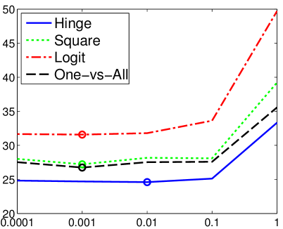
(a) $L/K=3$ (errors vs $\alpha$)

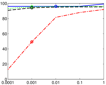
(b) $L/K=3$ (sparsity vs $\alpha$)

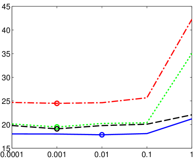
(c) $L/K=5$ (errors vs $\alpha$)

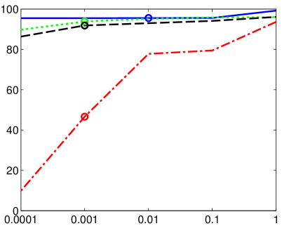
(d) $L/K=5$ (sparsity vs $\alpha$)

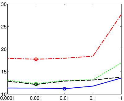
(e) $L/K=10$ (errors vs $\alpha$)

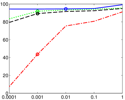
(f) $L/K=10$ (sparsity vs $\alpha$)

Figure 1: Results on MNIST database with the $\boldsymbol{\ell}_{1,\infty}$-regularization for $L\in\{3K,5K,10K\}$. Left column: classification errors as a function of $\alpha$. Right column: percentage of zero coefficients in vectors $({\rm x}^{(k)})_{1\leq k\leq K}$ as a function of $\alpha$. The circles mark the values yielding the best accuracy.

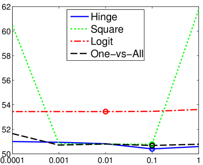
(a) $L/K=5$ (errors vs $\alpha$)

(b) $L/K=5$ (sparsity vs $\alpha$)

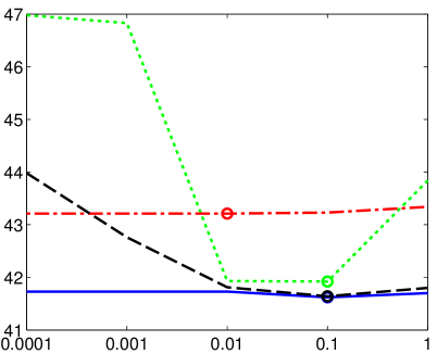
(c) $L/K=10$ (errors vs $\alpha$)

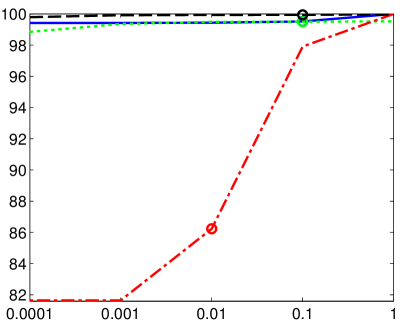
(d) $L/K=10$ (sparsity vs $\alpha$)

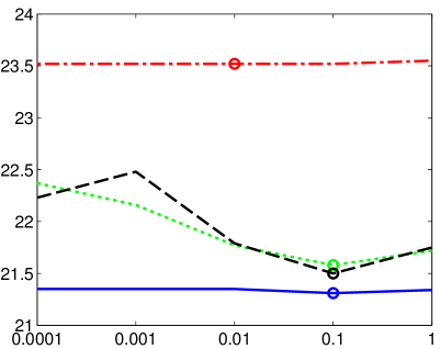
(e) $L/K=50$ (errors vs $\alpha$)

(f) $L/K=50$ (sparsity vs $\alpha$)

Figure 2: Results on News20 database with the $\boldsymbol{\ell}_{1,2}$-regularization for $L\in\{5K,10K,50K\}$. Left column: classification errors as a function of $\alpha$. Right column: percentage of zero coefficients in vectors $({\rm x}^{(k)})_{1\leq k\leq K}$ as a function of $\alpha$. The circles mark the values yielding the best accuracy.

4.2 Assessment of execution times

In this section, we compare the execution times of Algorithms 1 and 2 with

• a FISTA implementation of Problem (19),
  

• a forward-backward implementation of Problem (20),
  

• a FBPD implementation of Problem (12) reformulated with linear constraints
  

  $$\underset{\begin{subarray}{c}{({\rm x},\zeta)\in\mathbb{R}^{(M+1)K}\times\mathbb{R}^{LK}}\end{subarray}}{\operatorname{minimize}}\;\;\;g({\rm x})\quad\operatorname{s.t.}\quad\begin{cases}&\displaystyle\sum_{\ell=1}^{L}\sum_{k=1}^{K}\zeta^{(\ell,k)}\leq K\eta,\\ &(\forall\ell\in\{1,...,L\})\quad\zeta^{(\ell,1)}=\dots=\zeta^{(\ell,K)},\\ &(\forall\ell\in\{1,...,L\})\quad\zeta^{(\ell,1)}\geq 0,\dots,\zeta^{(\ell,K)}\geq 0,\\ &(\forall\ell\in\{1,...,L\})\quad T_{\ell}\,{\rm x}+r_{\ell}-(\zeta^{(\ell,k)})_{1\leq k\leq K}\leq 0.\end{cases}$$

  This approach is conceptually similar to the linear programming methods proposed by [33] and [37] for $\boldsymbol{\ell}_{1}$- or $\boldsymbol{\ell}_{1,+\infty}$-regularized SVMs.

Figures 3a, 3c and 3e show the execution times (averaged among $10$ training sets) obtained by the above algorithms for various values of $\lambda$ and $\eta$ on the MNIST database with $L\in\{3K,5K,10K\}$. In this experiment, the execution times refer to a stopping criterion of $10^{-5}$ on the relative error between two consecutive iterates. Conversely, Figures 3b, 3d and 3f show the relative distance to $\|{\rm x}^{[i]}-{\rm x}^{[\infty]}\|/\|{\rm x}^{[\infty]}\|$ (as a function of time) for the values of $\lambda$ and $\eta$ yielding the best accuracy (as reported in Figure 1), where ${\rm x}^{[\infty]}$ denotes the solution computed with a stopping criterion of $10^{-5}$. These results demonstrate that the proposed algorithms are faster than the approaches based on linear constraints and logistic regression, while being comparable in terms of execution times to approaches based on the square hinge loss. In addition, Algorithm 2 turns out to converge faster than Algorithm 1. This can be explained by the higher computational cost of the projection onto the standard simplex.

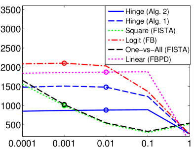
(a) $L/K=3$ (average time vs $\alpha$)

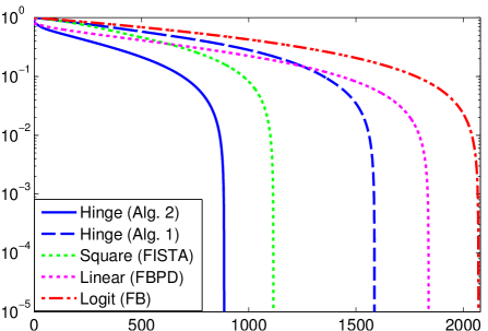
(b) $L/K=3$ (distance vs time)

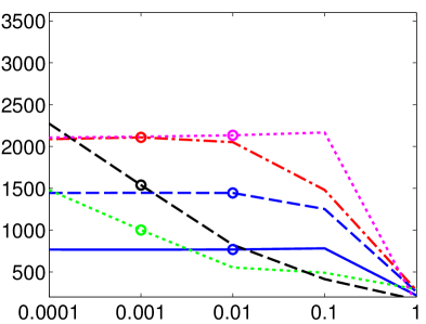
(c) $L/K=5$ (average time vs $\alpha$)

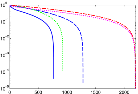
(d) $L/K=5$ (distance vs time)

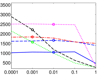
(e) $L/K=10$ (average time vs $\alpha$)

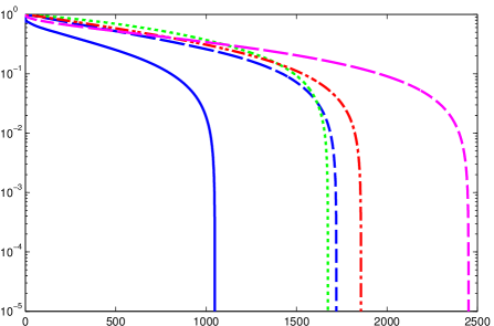
(f) $L/K=10$ (distance vs time)

Figure 3: Results on MNIST database with the $\boldsymbol{\ell}_{1,\infty}$-regularization for $L\in\{3K,5K,10K\}$. Left column: execution time as a function of $\alpha$, where the circles mark the values yielding the best accuracy (as reported in Figure 1). Right column: distance to ${\rm x}^{[\infty]}$ (as a function of time) obtained with the values of $\alpha$ marked by a circle in the left column (note that the one-vs-all approach, being defined by multiple optimization problems, does not allow us to determine the iterate $x^{[i]}$ at each iteration, hence the associated plot cannot be traced).

4.3 Quadratic regularization

Although our emphasis is on sparse learning, we propose to complete our analysis by evaluating the efficiency of the proposed algorithms in the case when $g$ is a quadratic regularization function. To this end, we compare the execution times of Algorithms 1 and 2 with the SVM-struct algorithm proposed by [6], which provides a numerical approach for solving Problem (4) through a cutting-plane technique. Figure 4 reports the execution times (averaged on $10$ training sets) obtained by the above methods on the MNIST database with $L\in\{3K,5K,10K,50K,100K,500K\}$ and different values of $\alpha$. In this experiment, we set the stopping criterion to $10^{-3}$ in all methods, and the regularization parameter of SVM-struct to $L/\alpha$. The results show that the proposed algorithms are competitive with state-of-the-art solutions in scenarios with a limited number of training data. The same cannot be claimed for larger databases, as SVM-struct scales particularly well w.r.t. the number $M$ of features and the size $L$ of the training set. Note however that, when $L/K=500$, the number of significant features for the SVM classifier designed with a quadratic regularization is equal to $M-546=158214$ (by setting a threshold to $10^{-5}$), while a sparse approach using an $\ell_{1,\infty}$-norm regularization yields only $42795$ nonzero features.

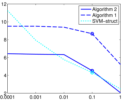
(a) $L/K=3$ (average time vs $\alpha$)

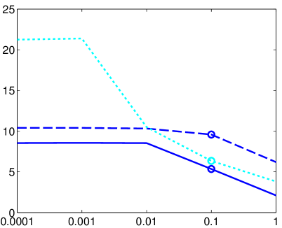
(b) $L/K=5$ (average time vs $\alpha$)

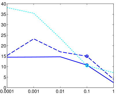
(c) $L/K=10$ (average time vs $\alpha$)

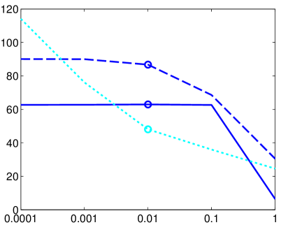
(d) $L/K=50$ (average time vs $\alpha$)

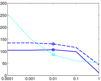
(e) $L/K=100$ (average time vs $\alpha$)

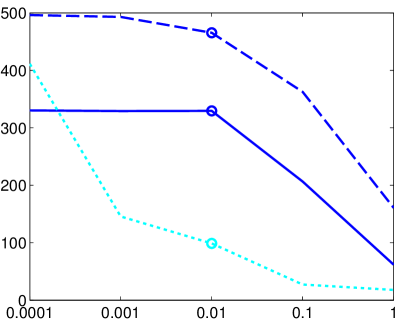
(f) $L/K=500$ (average time vs $\alpha$)

Figure 4: Results on MNIST database with a quadratic regularization. The plots show the execution times obtained with a stopping criterion of $10^{-3}$ for some values of $\alpha$. The circles mark the values of $\alpha$ yielding the best classification accuracy.

5 Conclusions

We have proposed two efficient algorithms for learning a sparse multiclass SVM. Our approach makes it possible to minimize a criterion involving the multiclass hinge loss and a sparsity-inducing regularization. In the literature, such a criterion is typically approximated by replacing the hinge loss with a smooth penalty, such as the quadratic hinge loss or the logistic loss. In this paper, we have provided two solutions that directly deal with the hinge loss: one addressing the regularized formulation and the other one adapted to the constrained formulation. The performance of the proposed solutions have been evaluated over three databases in scenarios with a few training data. The results show that the use of the hinge loss, rather than an approximation, leads to a slightly better classification accuracy and tends to make the method more robust w.r.t. the choice of the regularization parameter, while the proposed algorithms are often faster than state-of-the-art solutions.

References

- [1] K. Crammer and Y. Singer, “On the algorithmic implementation of multiclass kernel-based vector machines,” Journal of Machine Learning Research, vol. 2, pp. 265–392, Jan. 2001.
- [2] D. Martín-Iglesias, J. Bernal-Chaves, C. Peláez-Moreno, A. Gallardo-Antolín, and F. Díaz-de María, “A speech recognizer based on multiclass SVMs with HMM-guided segmentation,” Nonlinear Analyses and Algorithms for Speech Processing, vol. 3817, pp. 257–266, 2005.
- [3] I. Tsochantaridis, T. Joachims, T. Hofmann, and Y. Altun, “Large margin methods for structured and interdependent output variables,” Journal of Machine Learning Research, vol. 6, pp. 1453–1484, 2005.
- [4] F. J. Huang and Y. LeCun, “Large-scale learning with SVM and convolutional for generic object categorization,” in Conference on Computer Vision and Pattern Recognition, New York, USA, 17-22 Jun. 2006, pp. 284–291.
- [5] I. Laptev, M. Marszalek, C. Schmid, and B. Rozenfeld, “Learning realistic human actions from movies,” in Conference on Computer Vision and Pattern Recognition, Anchorage, AK, 23-28 June 2008, pp. 1–8.
- [6] T. Joachims, T. Finley, and C.-N. J. Yu, “Cutting-plane training of structural SVMs,” Machine Learning, vol. 77, no. 1, pp. 27–59, Oct. 2009.
- [7] C. Cortes and V. Vapnik, “Support-vector networks,” Machine Learning, vol. 20, no. 3, pp. 273–297, Sept. 1995.
- [8] M. Aizerman, E. Braverman, and L. Rozonoer, “Theoretical foundations of the potential function method in pattern recognition learning,” Automation and Remote Control, vol. 25, pp. 821–837, 1964.
- [9] J. C. Platt, “Fast training of support vector machines using sequential minimal optimization,” in Advances in Kernel Methods - Support Vector Learning, B. Schölkopf, C. J. C. Burges, and A. J. Smola, Eds., pp. 185–208. MIT Press, Cambridge, USA, Jan. 1998.
- [10] M. Blondel, A. Fujino, and N. Ueda, “Large-scale multiclass support vector machine training via euclidean projection onto the simplex,” in International Conference on Pattern Recognition, Stockholm, Sweden, 24-28 August 2014, pp. 1289–1294.
- [11] B. Krishnapuram, L. Carin, M. A. T. Figueiredo, and A. J. Hartemink, “Sparse multinomial logistic regression: Fast algorithms and generalization bounds,” IEEE Trans. on Pattern Analysis and Machine Intelligence, vol. 27, no. 6, June 2005.
- [12] J. Duchi and Y. Singer, “Boosting with structural sparsity,” in International Conference on Machine Learning, Montreal, Canada, 14-18 June 2009, pp. 297–304.
- [13] G.-X. Yuan, K.-W. Chang, C.-J. Hsieh, and C.-J. Lin, “A comparison of optimization methods and software for large-scale L1-regularized linear classification,” Machine Learning, vol. 11, pp. 3183–3234, Dec. 2010.
- [14] A. Rakotomamonjy, R. Flamary, G. Gasso, and S. Canu, “ penalty for sparse linear and sparse multiple kernel multi-task learning,” IEEE Trans. on Neural Networks, vol. 22, no. 8, pp. 1307–1320, Aug. 2011.
- [15] F. Bach, R. Jenatton, J. Mairal, and G. Obozinski, “Optimization with sparsity-inducing penalties,” Foundations and Trends in Machine Learning, vol. 4, no. 1, pp. 1–106, Jan. 2012.
- [16] L. Rosasco, S. Villa, S. Mosci, M. Santoro, and A. Verri, “Nonparametric sparsity and regularization,” Journal of Machine Learning Research, vol. 14, pp. 1665−–1714, July 2013.
- [17] D. Tuia, M. Volpi, M. Dalla Mura, A. Rakotomamonjy, and R. Flamary, “Automatic feature learning for spatio-spectral image classification with sparse SVM,” IEEE Trans. on Geoscience and Remote Sensing, vol. 52, no. 10, pp. 6062–6074, Oct. 2014.
- [18] S. Villa, L. Rosasco, S. Mosci, and A. Verri, “Proximal methods for the latent group lasso penalty,” Computational Optimization and Applications, vol. 58, no. 2, pp. 381–407, Dec. 2014.
- [19] B. C. Vũ, “A splitting algorithm for dual monotone inclusions involving cocoercive operators,” Advances in Computational Mathematics, vol. 38, no. 3, pp. 667–681, Apr. 2013.
- [20] L. Condat, “A primal-dual splitting method for convex optimization involving Lipschitzian, proximable and linear composite terms,” Journal of Optimization Theory and Applications, vol. 158, no. 2, pp. 460–479, Aug. 2013.
- [21] G. Chierchia, N. Pustelnik, J.-C. Pesquet, and B. Pesquet-Popescu, “Epigraphical projection and proximal tools for solving constrained convex optimization problems,” Signal, Image and Video Processing, July 2014.
- [22] G. Chierchia, N. Pustelnik, J.-C. Pesquet, and B. Pesquet-Popescu, “Epigraphical proximal projection for sparse multiclass SVM,” in International Conference on Acoustics, Speech and Signal Processing, Florence, Italy, 4-9 May 2014.
- [23] P. S. Bradley and O. L. Mangasarian, “Feature selection via concave minimization and support vector machines,” in International Conference on Machine Learning, Madison, USA, 1998, pp. 82–90.
- [24] J. Weston, A. Elisseeff, B. Schölkopf, and M. Tipping, “Use of the zero-norm with linear models and kernel methods,” Machine Learning, vol. 3, pp. 1439–1461, 2002.
- [25] Y. Liu, H. Helen Zhang, C. Park, and J. Ahn, “Support vector machines with adaptive Lq penalty,” Computational Statistics and Data Analysis, vol. 51, no. 12, pp. 6380–6394, Aug. 2007.
- [26] H. Zou and M. Yuan, “The f∞-norm support vector machine,” Statistica Sinica, vol. 18, pp. 379–398, 2008.
- [27] Y. Liu and Y. Wu, “Variable selection via a combination of the L0 and L1 penalties,” Journal of Computational and Graphical Statistics, vol. 14, no. 4, pp. 782–798, Dec. 2007.
- [28] L. Wang, J. Zhu, and H. Zou, “The doubly regularized support vector machine,” Statistica Sinica, vol. 16, pp. 589–616, 2006.
- [29] M. Tan, L. Wang, and I. W. Tsang, “Learning sparse SVM for feature selection on very high dimensional datasets,” in International Conference on Machine Learning, Haifa, Israel, 21-24 June 2010, pp. 1047–1054.
- [30] L. Laporte, R. Flamary, S. Canu, S. Déjean, and J. Mothe, “Non-convex regularizations for feature selection in ranking with sparse SVM,” IEEE Trans. on Neural Networks and Learning Systems, vol. 25, no. 6, pp. 1118 – 1130, June 2014.
- [31] E. J. Candés, M. B. Wakin, and S. Boyd, “Enhancing sparsity by reweighted minimization,” Journal of Fourier Analysis and Applications, vol. 14, no. 5, pp. 877–905, Dec. 2008.
- [32] R. Rifkin and A. Klautau, “In defense of one-vs-all classification,” Machine Learning, vol. 5, pp. 101–141, 2004.
- [33] L. Wang and X. Shen, “On -norm multi-class support vector machines: methodology and theory,” Journal of the American Statistical Association, vol. 102, pp. 583–594, 2007.
- [34] M. Yuan and Y. Lin, “Model selection and estimation in regression with grouped variables,” Journal of the Royal Statistical Society: Series B, vol. 68, pp. 49–67, 2006.
- [35] L. Meier, S. Van De Geer, and P. Bühlmann, “The group Lasso for logistic regression,” Journal of the Royal Statistical Society: Series B, vol. 70, no. 1, pp. 53–71, 2008.
- [36] G. Obozinski, B. Taskar, and M. I. Jordan, “Joint covariate selection and joint subspace selection for multiple classification problems,” Statistics and Computing, vol. 20, no. 2, pp. 231–252, 2010.
- [37] H.H. Zhang, Y. Liu, Y. Wu, and J. Zhu, “Variable selection for multicategory SVM via sup-norm regularization,” Electronic Journal of Statistics, vol. 2, pp. 149–167, 2008.
- [38] M. Blondel, K. Seki, and K. Uehara, “Block coordinate descent algorithms for large-scale sparse multiclass classification,” Machine Learning, vol. 93, no. 1, pp. 31–52, Oct. 2013.
- [39] T. M. Cover, “Geometrical and statistical properties of systems of linear inequalities with applications in pattern recognition,” IEEE Trans. on Electronic Computers, vol. EC-14, no. 3, pp. 326–334, June 1965.
- [40] S. Boyd and L. Vandenberghe, Convex Optimization, Cambrige University Press, Cambridge, UK, 2004.
- [41] P. L. Combettes and J.-C. Pesquet, “Proximal splitting methods in signal processing,” in Fixed-Point Algorithms for Inverse Problems in Science and Engineering, H. H. Bauschke, R. S. Burachik, P. L. Combettes, V. Elser, D. R. Luke, and H. Wolkowicz, Eds., pp. 185–212. Springer-Verlag, New York, 2011.
- [42] P. L. Combettes and J.-C. Pesquet, “Primal-dual splitting algorithm for solving inclusions with mixtures of composite, Lipschitzian, and parallel-sum type monotone operators,” Set-Valued and Variational Analysis, vol. 20, no. 2, pp. 307–330, June 2012.
- [43] N. Parikh and S. Boyd, “Proximal algorithms,” Foundations and Trends in Optimization, vol. 1, no. 3, pp. 123–231, 2014.
- [44] N. Komodakis and J.-C. Pesquet, “Playing with duality: An overview of recent primal-dual approaches for solving large-scale optimization problems,” IEEE Signal Processing Magazine, 2014, accepted for publication.
- [45] J. J. Moreau, “Proximité et dualité dans un espace hilbertien,” Bulletin de la Société Mathématique de France, vol. 93, pp. 273–299, 1965.
- [46] A. Chambolle and T. Pock, “A first-order primal-dual algorithm for convex problems with applications to imaging,” Journal of Mathematical Imaging and Vision, vol. 40, no. 1, May 2011.
- [47] P. L. Combettes, L. Condat, J.-C. Pesquet, and B. C. Vũ, “A forward-backward view of some primal-dual optimization methods in image recovery,” in International Conference on Image Processing, Paris, France, 27-30 October 2014.
- [48] P. L. Combettes and B. C. Vũ, “Variable metric forward-backward splitting with applications to monotone inclusions in duality,” Optimization, vol. 63, no. 9, pp. 1289–1318, Sept. 2014.
- [49] L. Condat, “Fast projection onto the simplex and the l1 ball,” 2014, Available online at http://hal.archives-ouvertes.fr/hal-01056171.
- [50] H. H. Bauschke and P. L. Combettes, Convex Analysis and Monotone Operator Theory in Hilbert Spaces, Springer, New York, 2011.
- [51] R. Gaetano, G. Chierchia, and B. Pesquet-Popescu, “Parallel implementations of a disparity estimation algorithm based on a proximal splitting method,” in Visual Communication and Image Processing, San Diego, USA, 27-30 November 2012, pp. 1–6.
- [52] T. H. Cormen, C. E. Leiserson, and R. L. Rivest, Introduction to Algorithms, MIT Press, 1990.
- [53] E. Van Den Berg and M. P. Friedlander, “Probing the Pareto frontier for basis pursuit solutions,” SIAM Journal on Scientific Computing, vol. 31, no. 2, pp. 890–912, Nov. 2008.
- [54] T. R. Golub, D. K. Slonim, P. Tamayo, C. Huard, M. Gaasenbeek, J. P. Mesirov, H. Coller, M. L. Loh, J. R. Downing, M. A. Caligiuri, C. D. Bloomfield, and E. S. Lander, “Molecular classification of cancer: Class discovery and class prediction by gene expression monitoring,” Science, vol. 286, no. 5439, pp. 531–537, 1999.
- [55] Y. LeCun, L. Bottou, Y. Bengio, and P. Haffner, “Gradient-based learning applied to document recognition,” Proceedings of IEEE, vol. 86, no. 11, pp. 2278–2324, Nov. 1998.
- [56] J. Bruna and S. Mallat, “Invariant scattering convolution networks,” IEEE Trans. on Pattern Analysis and Machine Intelligence, vol. 35, no. 8, pp. 1872–1886, Aug. 2013.
- [57] K. Lang, “Newsweeder: Learning to filter netnews,” in International Conference on Machine Learning, Tahoe City, USA, 9-12 July 1995, pp. 331–339.
- [58] T. Joachims, “Text categorization with suport vector machines: Learning with many relevant features,” in European Conference on Machine Learning, Chemnitz, Germany, 21-24 April 1998, pp. 137–142.