Coherent quantum squeezing due to the phase space noncommutativity

Abstract

The effect of phase space general noncommutativity on producing deformed coherent squeezed states is examined. A two-dimensional noncommutative quantum system supported by a deformed mathematical structure similar to that of Hadamard billiards is obtained and their components behavior are monitored in time. It is assumed that the independent degrees of freedom are two free 1D harmonic oscillators (HO’s), so the system Hamiltonian does not contain interaction terms. Through the noncommutative deformation parameterized by a Seiberg-Witten transform on the original canonical variables, one gets the standard commutation relations for the new ones, such that the obtained Hamiltonian represents then two interacting 1D HO’s. By assuming that one HO is inverted relatively to the other, it is shown that their effective interaction induces a squeezing dynamics for initial coherent states imaged in the phase space. A suitable pattern of logarithmic spirals is obtained and some relevant properties are discussed in terms of Wigner functions, which are essential to put in evidence the effects of the noncommutativity.

I Introduction

Supported by a deformed Heisenberg-Weyl algebra Catarina ; 06A ; 07A ; 08A ; 09A ; Gamboa ; Guisado , the phase space noncommutative generalization of quantum mechanics (QM) provides some elementary responses to typical issues which circumvent the intersection between quantum and classical mechanics. Besides evincing the role of noncommutativity in the predictions of the standard QM, some emblematic quantum effects like quantum decoherence, quantum entanglement Bernardini13B , and the collapse of the wave function Bernardini13A can be indeed fine-tuned to work as a probe of noncommutativity imprints on QM.

Even if it has been lately focused on studies of the quantum Hall effect Prange , on the spectroscopy of the gravitational quantum well for ultra-cold neutrons 06A , on the Landau level and 2D harmonic oscillator problems in the phase space Nekrasov01 ; Rosenbaum ; Bernardini13A , and on quantumness and entanglement-separability issues Bernardini13B , the noncommutativity is also believed to be a regular feature of quantum gravity and string theory Snyder47 ; Connes ; Seiberg . Likewise, besides providing consistent explanations for the black hole singularity Bastos3 in the framework of quantum cosmology, the noncommutative QM scenario includes possible extensions of the matrix formulation of the uncertainty principle Ber2014 , and it has also stimulated a constructive analysis of the equivalence principle Bastos4 . The framework is modeled on a $2n$-dimensional phase space where the time variable is assumed as a commutative parameter, and the phase space coordinate commutation relations are supported by a noncommutative algebra, in manner that a noncommutative formulation of QM is more suitably stablished in terms of the Weyl-Wigner-Groenewald-Moyal (WWGM) formalism Groenewold ; Moyal ; Wigner .

In this contribution, the role of the noncommutative algebra of two free harmonic oscillators (HO’s) (described by a Hamiltonian with a quadratic structure involving the phase space variables, positions and momenta) on producing squeezing is discussed through an analysis based on a time-evolving Wigner function. A Seiberg-Witten transform on the noncommutative variables Seiberg leads a novel set of (now canonical) variables which exhibit the standard commutation relations of Weyl-Heisenberg algebra, at the price that now the HO’s are not more free, and they interact through the emergence of an additional term in the Hamiltonian. Thus, this procedure allows one to determine how the noncommutative parameters induce the squeezing dynamics for initial coherent states by the arising of a specific interaction. The other way around, one could say that two interacting HO’s in QM are equivalent to two free ones whose phase space variables follow a generalized noncommutative algebra. Last but not least, it is worth reminding that the system can be circumstantially identified with a Hadamard dynamical system Hadamard .

II The noncommutative algebra of a dynamical system

The Hamiltonian formulation of 2D quantum mechanical problems correspond to the most accessible systems for which the noncommutative phase space properties can be probed Nekrasov01 ; Rosenbaum ; Bernardini13A . Therefore, one considers two 1D HO’s sliding frictionlessly, and having the Hamiltonian,

$${H}(\mathbf{q},\mathbf{p})=\sum_{i,j=1}^{2}g^{ij}\left(\frac{1}{2m}\,p_{i}p_{j}+\frac{1}{2}m\omega^{2}\,q_{i}q_{j}\right),$$ (1)

where the operator vector notation is set as $\mathbf{v}=({v}_{1},{v}_{2})$, and $g^{ij}$ is the metric tensor on the manifold. Through a particular choice of the Riemann manifold parameterized by $g^{ij}$, the above Hamiltonian can be converted into suitable probe of noncommutative effects. One thus sets $g^{ij}=\delta^{i1}\delta^{j2}+\delta^{i2}\delta^{j1}$ such that it shall then represent a pair of $45$ degrees rotated decoupled HO’s, one with corresponding energy spectrum unbounded from below, and another with energy spectrum unbounded from above. This problem was treated in a different context by R. J. Glauber in Glauber . In fact, by identifying the $1D$ harmonic oscillator Hamiltonian with

$${H}_{HO}(x_{j},k_{j})=\frac{1}{2m}\,k_{j}^{\mbox{\tiny$2$}}+\frac{1}{2}m\omega^{2}\,x_{j}^{\mbox{\tiny$2$}},$$ (2)

with $x_{j}=(q_{1}-(-1)^{j}q_{2})/\sqrt{2}$ and $k_{j}=(p_{1}-(-1)^{j}p_{2})/\sqrt{2}$, with $j=1,\,2$, one has

$${H}(\mathbf{q},\mathbf{p})\equiv{H}_{HO}(x_{1},k_{1})-{H}_{HO}(x_{2},k_{2})\equiv{H}_{HO}(x_{1},k_{1})+{H}_{HO}(i\,x_{2},i\,k_{2}),$$ (3)

where the last passage indicates that the system labeled by $j=2$ can be read as a Hamiltonian component that is presumed to have its position and momentum coordinates driven by a Wick rotation, which turns a bounded Hamiltonian into an unbounded one, from below. Globally, it corresponds to change a spherical manifold, namely the simplest compact Riemann surface with positive curvature, into a hyperbolic manifold, by the way, a compact Riemann surface with negative curvature.

One shall notice that the noncommutative deformation induces some modifications that allow one to overcome the infinities and divergent behaviors originated from the above Hamiltonian dynamics. The spatial and momentum noncommutative algebra is set as

$$\left[{q}_{i},{q}_{j}\right]=i\theta\epsilon_{ij}\hskip 5.69046pt,\hskip 5.69046pt\left[{q}_{i},{p}_{j}\right]=i\delta_{ij}\hbar,\hskip 5.69046pt\left[{p}_{i},{p}_{j}\right]=i\eta\epsilon_{ij}\hskip 5.69046pt,\hskip 5.69046pti,j=1,2,$$ (4)

with the Levi-Civita tensor $\epsilon_{ij}=-\epsilon_{ji}$, such that the Seiberg-Witten (SW) Seiberg map to the commutative operators, $\{\mbox{\bf\em Q},\mathbf{\Pi}\}$, can be read as

$${q}_{i}=\lambda\mathit{{Q}}_{i}-\frac{\theta}{2\lambda\hbar}\sum_{j=1}^{2}\epsilon_{ij}{\Pi}_{j}\hskip 14.22636pt,\hskip 14.22636pt{p}_{i}=\mu{\Pi}_{i}+\frac{\eta}{2\mu\hbar}\sum_{j=1}^{2}\epsilon_{ij}\mathit{{Q}}_{j}\leavevmode\nobreak\ ,$$ (5)

which is invertible when a constraint on the dimensionless parameters $\lambda$ and $\mu$ is stablished by the relation Catarina

$$\frac{\theta\eta}{4\hbar^{2}}=\lambda\mu(1-\lambda\mu),$$ (6)

as to have the corresponding Jacobian given by

$$\left\|\frac{\partial({q},{p})}{\partial({\mathit{Q}},{\Pi})}\right\|=(\det{\mathbf{\Omega}})^{1/2}=1-\frac{\theta\eta}{\hbar^{2}},$$ (7)

with

$$\mathbf{\Omega}=\left[\begin{array}[]{cccc}0&+\theta/\hbar&+1&0\\ -\theta/\hbar&0&0&+1\\ -1&0&0&+\eta/\hbar\\ 0&-1&-\eta/\hbar&0\end{array}\right],$$

where $0\leq\theta\eta<\hbar^{2}$. One thus obtains the inverse map given by Catarina

$$\mathit{{Q}}_{i} = \mu\left(1-\frac{\theta\eta}{\hbar^{2}}\right)^{-1/2}\left({q}_{i}+\frac{\theta}{2\lambda\mu\hbar}\sum_{j=1}^{2}\epsilon_{ij}{p}_{j}\right),$$

$${\Pi}_{i} = \lambda\left(1-\frac{\theta\eta}{\hbar^{2}}\right)^{-1/2}\left({p}_{i}-\frac{\eta}{2\lambda\mu\hbar}\sum_{j=1}^{2}\epsilon_{ij}{q}_{j}\right),$$ (8)

which guarantees that the new coordinates satisfy the standard Weyl-Heisenberg algebra,

$$\left[{Q}_{i},{Q}_{j}\right]=\left[{\Pi}_{i},{\Pi}_{j}\right]=0\qquad\mbox{and}\qquad\left[{Q}_{i},{\Pi}_{j}\right]=i\delta_{ij}\hbar,\hskip 5.69046pti,j=1,2,$$ (9)

such that the Hamiltonian of the previously uncoupled HO’s can be re-written in terms of the new variables, $\mathit{{Q}}_{i}$ and ${\Pi}_{i}$, as

$$H(\mbox{\bf\em Q},\mathbf{\Pi})=\sum_{i,j=1}^{2}g^{ij}\,\left(\alpha^{2}\mathit{{Q}}_{i}\mathit{{Q}}_{j}+\beta^{2}{\Pi}_{i}{\Pi}_{j}\right)+\frac{\Gamma}{2}\left(\left\{\mathit{{Q}}_{1},\ {\Pi}_{1}\right\}-\left\{\mathit{{Q}}_{2},\ {\Pi}_{2}\right\}\right),$$ (10)

with

$${\alpha}^{2} \equiv \frac{\lambda^{2}m\omega^{2}}{2}-\frac{\eta^{2}}{8m\mu^{2}\hbar^{2}}\leavevmode\nobreak\ ,$$ (11)

$${\beta}^{2} \equiv \frac{\mu^{2}}{2m}-\frac{m\omega^{2}\theta^{2}}{8\lambda^{2}\hbar^{2}}\leavevmode\nobreak\ ,$$ (12)

where, preliminarily assuming that the constraint (6) is satisfied, the positiveness of ${\alpha}^{2}$ and ${\beta}^{2}$ are independently and phenomenologically assumed ad hoc, with the consequences of (6) straightforwardly extended to the choice of the parameters $\lambda$ and $\mu$, and with

$${\Gamma}\equiv\frac{\theta}{2\hbar}m\omega^{2}-\frac{\eta}{2m\hbar},$$ (13)

the parameter that couples the HO’s. The Hamiltonian remains unbounded in the noncommutative scenario, however, the noncommutative algebra from Eq.(4)induces an additional coupling between the unbounded subsystems mediated by the parameter $\Gamma$, as to have an isentropic system with globally conserved energy flows recursively absorbed from the one to the other, as it shall be depicted from the solutions of the equations of motion.

Since Q and $\mathbf{\Pi}$ satisfy Hamilton equations of motion, one has the following set of coupled first-order differential equations,

$$\dot{\Pi}_{k} = -\frac{i}{\hbar}\left[\Pi_{k},\,H\right]=\leavevmode\nobreak\ \leavevmode\nobreak\ (-1)^{k}\,\left(2\alpha^{2}\,\sum_{j=1}^{2}\epsilon_{kj}\mathit{Q}_{j}+\Gamma\,\Pi_{k}\right),$$

$$\dot{\mathit{Q}}_{k} = -\frac{i}{\hbar}\left[\mathit{Q}_{k},\,H\right]=-(-1)^{k}\,\left(2\beta^{2}\,\sum_{j=1}^{2}\epsilon_{kj}\Pi_{j}+\Gamma\,\mathit{Q}_{k}\right),\qquad k=1,2.$$ (14)

After simple mathematical manipulations, the above equations can be written as two uncoupled second-order differential equations,

$$\ddot{\Pi}_{k}-(-1)^{k}\,2\Gamma\,\dot{\Pi}_{k}+(\Gamma^{2}+4\alpha^{2}\beta^{2})\,\Pi_{k} = 0,$$

$$\ddot{\mathit{Q}}_{k}+(-1)^{k}\,2\Gamma\,\dot{\mathit{Q}}_{k}+(\Gamma^{2}+4\alpha^{2}\beta^{2})\,\mathit{Q}_{k} = 0,$$ (15)

from which one gets the dynamical variables,

$$\mathit{Q}_{1}(t) = \exp{(+\Gamma t)}\left[x\,\cos(\Omega t)+\frac{\beta}{\alpha}\pi_{y}\,\sin(\Omega t)\right],$$ (16a)

$$\mathit{Q}_{2}(t) = \exp{(-\Gamma t)}\left[y\,\cos(\Omega t)+\frac{\beta}{\alpha}\pi_{x}\,\sin(\Omega t)\right],$$ (16b)

$$\Pi_{1}(t) = \exp{(-\Gamma t)}\left[\pi_{x}\,\cos(\Omega t)-\frac{\alpha}{\beta}y\,\sin(\Omega t)\right],$$ (16c)

$$\Pi_{2}(t) = \exp{(+\Gamma t)}\left[\pi_{y}\,\cos(\Omega t)-\frac{\alpha}{\beta}x\,\sin(\Omega t)\right],$$ (16d)

where $x=Q_{1}(0),\,y=Q_{2}(0),\,\pi_{x}=\Pi_{1}(0),$ and $\pi_{y}=\Pi_{2}(0)$ are the initial conditions, and

$$\Omega=2\alpha\beta=\omega\sqrt{(2\lambda\mu-1)^{2}-\varepsilon^{2}},$$ (17)

with

$$\varepsilon=\frac{1}{2\hbar}\left[m\omega\theta-\frac{\eta}{m\omega}\right],$$ (18)

so that $\Gamma=\omega\varepsilon$. Notice that the mathematical structure of the above results is very similar to that from Ref. Bernardini13A , for which a $2D$ noncommutative HO is discussed. One observes that, for $\varepsilon>0$, one variable (for each HO) is amplified as time goes on whereas the other is attenuated, such that the commutation relations remain unaffected, $\left[Q_{i}(t),\Pi_{j}(t)\right]=i\hbar\delta_{ij}$. By setting $\varepsilon=0$ one recovers the solutions for the uncoupled HO’s coordinates. For $0<\varepsilon\ll 1$, one has

$$\Omega\sim\omega[1+\mathcal{O}(\varepsilon^{2})]\times|2\lambda\mu-1|\sim\omega[1+\mathcal{O}(\theta^{2},\,\eta^{2},\,\theta\eta)],$$

and the noncommutative parameters, $\theta$ and $\eta$, introduce second-order corrections in $\Omega$ (c. f. Ref. Bernardini13A ). Likewise, the modifications due to $\Gamma=\omega\varepsilon$ correspond to typical first order effects as quantified in Refs. Catarina ; Bernardini13A .

III Phase space and Wigner function

The time evolution within the phase space associated with the operators $(\mathit{Q}_{1}(t),\Pi_{1}(t))$ and $(\mathit{Q}_{2}(t),\Pi_{2}(t))$ are depicted in Fig. 1, for which the time is in the range $[0,2\pi/\Omega]$. For convenience, the auxiliary variable

$$\epsilon=\frac{\Gamma}{\Omega}=\frac{\varepsilon}{\sqrt{(2\lambda\mu-1)^{2}-\varepsilon^{2}}},$$ (19)

is defined to be used for a non-perturbative analysis of the results. The phase space maps from the first and second columns in Fig. 1 correspond, respectively, to direct and indirect logarithmic spirals which are associated to damping and amplifying modes. Two examples for which one identifies different choices of the set of initial conditions are presented. Considering only one separated HO, one gets it as an open (unbounded from below Hamiltonian, or even non-Hamiltonian) system. To reestablish the canonical formalism and conservation of information, one must have both HO’s in order to have a closed and isentropic system.

The dynamical evolution of a wavefunction or a density operator can be mapped into a Wigner function (WF), $W(\mbox{\bf\em Q},\mathbf{\Pi})$ (now on the variables $\bf{Q}$ and $\bf{P}$ are c-numbers), since one can follow trajectories of the motion in the phase space. One has only to ensure that each point of the WF moves in the correlated paths, $1\leftrightarrow 2$, as depicted for instance in the plots from Fig. 1. This is reflected by a characteristic invariance property of stationary WFs. The time evolution of a WF is given by a propagator acting on an “initial” one,

$$W(\mathbf{Q},\mathbf{\Pi},t)=e^{-i\mathcal{L}_{Q}(t-t_{0})}W(\mathbf{Q},\mathbf{\Pi},t_{0}),$$ (20)

where

$$\mathcal{L}_{Q}\equiv H\left(\mathbf{Q},\mathbf{\Pi}\right)\left[i\frac{2}{\hbar}\sin\left(\frac{\hbar}{2}\overleftrightarrow{\Lambda}\right)\right],$$ (21)

is the Liouvillian superoperator, $H\left(\mathbf{Q},\mathbf{\Pi}\right)$ is Weyl’s map of the Hamiltonian operator, and

$$\overleftrightarrow{\Lambda}=\frac{\overleftarrow{\partial}}{\partial{\mathbf{Q}}}\cdot\frac{\overrightarrow{\partial}}{\partial{\mathbf{\Pi}}}-\frac{\overleftarrow{\partial}}{\partial{\mathbf{\Pi}}}\cdot\frac{\overrightarrow{\partial}}{\partial{\mathbf{Q}}},$$ (22)

is an operator acting on the left on $H\left(\mathbf{Q},\mathbf{\Pi}\right)$ and on the right on the WF. For a quadratic Hamiltonian, the Liouvillian reduces to

$$\mathcal{L}_{cl}=iH\left(\mathbf{Q},\mathbf{\Pi}\right)\overleftrightarrow{\Lambda},$$ (23)

resulting in a classical evolution (this is another form of the Ehrenfest theorem) BMT1 ; BMT2 . Thus, assuming $t_{0}=0$,

$$W(\mathbf{Q},\mathbf{\Pi},t) = e^{-i\mathcal{L}_{cl}(t)}W(\mathbf{Q},\mathbf{\Pi},0)$$ (24)

$$= W(e^{i\mathcal{L}_{cl}(t)}\mathbf{Q}(0),\ e^{i\mathcal{L}_{cl}(t)}\mathbf{\Pi}(0),0)=W(\mathbf{Q}(-t),\mathbf{\Pi}(-t),0),$$

using the time reversed solutions of Eqs. (16), with the q-numbers being substituted by c-numbers, and reminding that $\left\{\mathit{Q}_{1}(0),\mathit{\Pi}_{1}(0),\mathit{Q}_{2}(0),\mathit{\Pi}_{2}(0)\right\}\equiv\left\{\mathit{x,\pi_{x},y,\pi_{y}}\right\}$.

It has been attributed to $W(\mathbf{Q},\mathbf{\Pi},0)$ a symmetric (non-squeezed) Gaussian form for both the HO’s, and one looks over to the time evolution of HO 1 only, getting the marginal Wigner functions $\tilde{W}^{(1)}(\mathit{Q}_{1},\mathit{\Pi}_{1};t)$ as shown in Fig. 2. As time goes on the WF evolves to a squeezed state, and the squeezing dynamics follows the logarithmic spiral evolution of the phase space variables (c. f. Fig. 1), and the results do not depend quantitatively on the parameter $\epsilon$ since one has chosen scale independent values for $\tau$.

IV Summary and discussions

The implications of noncommutativity of the dynamical variables of two free HO’s on producing squeezing states has been established. This feature is observed when a Seiberg-Witten transform is applied on the variables, thus coupling the HO’s. The squeezing observed in each HO occurs by a phase difference of $\pi$, due to the different exponential factor in Eqs. (16).

Looking at only one HO, the missing information is completely absorbed by the other, once it flows recursively from the one to the other although it is globally conserved, since the system is isentropic, as it was already discussed, in a similar context, for two interacting modes of the electromagnetic field, in Refs. OMD ; CDM .

Our results also reinforce previous analysis where the noncommutative effects of variables can be considered when addressing the issues of the fine tuning of quantum effects. Squeezing and quantum dissipation properties Cel01 ; Cel02 and a set of analogous results outside the scope of the noncommutative can also be found in the study of a $SU(1,1)$ structure of squeezed states as damped oscillators Cel03 dynamically generated by single-mode hamiltonians characterized by two-photon process interactions, with damping elements similar to that exhibited by Eq. (10). Recently, the self-similarity properties of fractals has been discussed in the context of the theory of entire analytical functions and of deformed algebra of coherent states Vitiello , and their functional realization in terms of squeezed coherent states has been obtained. The noncommutativity in the phase space reported in this paper changes the similar dynamics of two uncoupled 1D HO’s (Hadamard’s billiard) into the dynamics of coupled logarithmic spirals.

The theoretical description supported by the noncommutativity in the phase space then supports a consistent explanation for several experimental observations of temporal large scale effects in superconductors, crystals, ferromagnets, etc Vitiello4 , where squeezed states also appear. As expected, the relevance of these results in terms of their experimental feasibility/detectability may depend essentially on the noncommutative parameters $\theta$ and $\eta$.

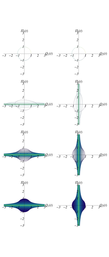
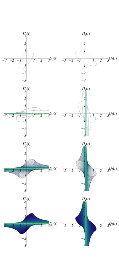
Figure 1: (Color online) Time evolution of the phase space coordinates,$(\mathit{Q}_{1}(t),\Pi_{1}(t))$ and $(\mathit{Q}_{2}(t),\Pi_{2}(t))$. The plots in the first line of each set (column) refer to the phase space elliptical orbits similar to those described for 2D harmonic oscillators (as if one had set $\epsilon=0$ in the noncommutative map). From the second to the forth plot lines one has set arbitrary values for $\epsilon$, $\epsilon=1/10,\,1/100$, and $1/1000$ respectively. Positive and time reversed logarithmic spirals describe the time-evolving open orbits for these cases. One has used a BlueGreenYellow (GrayLevel) scale in order to denote the time scale, $\tau$, varying from $0$ (blue (dark gray)) to $2\pi/\Omega$ (yellow (light gray)), such that orbits start and finish at $(x,\pi_{x},y,\pi_{y})$ equals to $(1,0,1,0)$ (first column) and $(1,1,1,0)$ (second column). By convenience, one has set $\alpha=\beta$, that is equivalent to $m\omega=\hbar=1$.

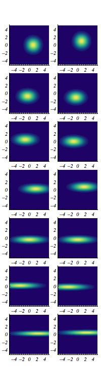
Figure 2: (Color online) Coherent quantum squeezing for Gaussian states in the $\mathit{Q}_{1}-\Pi_{1}$ plane, which evolves in correspondence with the phase space map depicted in Fig. 1. At time $\tau=0$ the Wigner function is assumed to be centered at departing points $(x,\pi_{x})$ from Fig. 1. One has considered time intervals such that $\tau=k\pi(32\epsilon\Omega)^{-1}$, with $k$ from $0$ to $6$, and $\epsilon=1/10$, in order to reproduce an equally spaced time evolution sequence of plots. The contour plot follows a BlueGreenYellow scale (from yellow (light gray) which corresponds to $1$, to blue (dark gray) which corresponds to $0$), from which the squeezing effect can be easily noticed.

- (1) C. Bastos, O. Bertolami, N. C. Dias and J. N. Prata, J. Math. Phys. 49, 072101 (2008).
- (2) O. Bertolami, J. G. Rosa, C. M. L. de Aragão, P. Castorina and D. Zappalà, Phys. Rev. D72, 025010 (2005).
- (3) O. Bertolami, J. G. Rosa, C. Aragão, P. Castorina and D. Zappalà, Mod. Phys. Lett. A 21, 795 (2006).
- (4) N. C. Dias and J. N. Prata, Annals Phys. 324, 73 (2009).
- (5) C. Bastos and O. Bertolami, Phys. Lett. A372, 5556 (2008).
- (6) J. Gamboa, M. Loewe and J. C. Rojas, Phys. Rev. D64, 067901 (2001); J. Gamboa et al., Mod. Phys. Lett. A16, 2075 (2001).
- (7) O. Bertolami, L. Guisado, JHEP 0312, 013 (2003).
- (8) C. Bastos, A. E. Bernardini, O. Bertolami, N. C. Dias and J. N. Prata, Phys. Rev. D88, 085013 (2013).
- (9) A. E. Bernardini and O. Bertolami, Phys. Rev. A 88 012101, (2013).
- (10) R. Prange and S. Girvin, The Quantum Hall Effect, (Springer, New York, 1987).
- (11) M. R. Douglas and N. A. Nekrasov, Rev. Mod. Phys. 73, 977 (2001).
- (12) M. Rosenbaum, J. David Vergara and L. Roman Juarez, Phys. Lett. A367, 1 (2007); M. Rosenbaum and J. David Vergara, Gen. Rel. Grav. 38, 607 (2006).
- (13) H. S. Snyder, Phys. Rev. 71, 38 (1947).
- (14) A. Connes, M. R. Douglas and A. Schwarz, JHEP 02, 003 (1998); M. R. Douglas and C. Hull, JHEP 02, 008 (1998); V. Schomerus, JHEP 9906, 030 (1999).
- (15) N. Seiberg and E. Witten, JHEP 9909, 032 (1999).
- (16) C.Bastos, O. Bertolami, N. C. Dias and J. Prata, Phys. Rev. D78, 023516 (2008); Phys. Rev. D80, 124038 (2009); Phys. Rev. D82, 041502 (2010); Phys. Rev. D84, 024005 (2011).
- (17) C. Bastos, A. E. Bernardini, O. Bertolami, N. C. Dias and J. N. Prata, Phys. Rev.D90, 045023 (2014).
- (18) C. Bastos, O. Bertolami, N. C. Dias and J. Prata, Class. Quant. Grav. 28, 125007 (2011).
- (19) H. Groenewold, Physica 12 (1946) 405.
- (20) J. E. Moyal, Proc. Camb. Phil. Soc. 45 (1949) 99.
- (21) E. Wigner, Phys. Rev. 40 (1932) 749.
- (22) J. Hadamard, Les surfaces à courbures opposées et leurs lignes géodésiques, J. Math. Pures et Appl. 4, 27 (1898).
- (23) R. J. Glauber, Ampifiers, Attenuators, and Schr dinger s Cat in “New Techniques and Ideas in Quantum Measurement Theory , Annals of the New York Academy of Science 480, 336 (1986).
- (24) G. Bund, S. S. Mizrahi, and M. C. Tijero, Phys. Rev. A 53, 1191 (1996).
- (25) G. Bund, S. S. Mizrahi, and M. C. Tijero, Phys. Rev. A 56, 2825 (1997).
- (26) M. C. de Oliveira, S. S. Mizrahi, and V. V. Dodonov, J. Opt. B: Quantum Semiclass. Opt. 1, 610 (1999).
- (27) A. S. M. de Castro, V. V. Dodonov, and S. S. Mizrahi, J. Opt. B: Quantum Semiclass. Opt. 4, S191 (2002).
- (28) E. Celeghini, M. Rasetti, and G. Vitiello, Phys. Rev. Lett. 66, 2056 (1991).
- (29) E. Celeghini, M. Rasetti, and G. Vitiello, Annals of Physics 215, 156 (1992).
- (30) E. Celeghini, M. Rasetti, M. Tarlini and G. Vitiello, Mod. Phys. Lett. B 3, 1213 (1989).
- (31) G. Vitiello, Phys. Lett. A 376, 2527 (2012).
- (32) Y. M. Bunkov, H. Godfrin, Topological Defects and the Nonequilibrium Dynamics of Symmetry Breaking Phase Transitions, Kluwer Academic Publ., Dordrecht, (2000).