A realizability-preserving discontinuous Galerkin scheme for entropy-based moment closures for linear kinetic equations in one space dimension

Abstract

We implement a high-order numerical scheme for the entropy-based moment closure, the so-called M_N model, for linear kinetic equations in slab geometry. A discontinuous Galerkin (DG) scheme in space along with a strong-stability preserving Runge-Kutta time integrator is a natural choice to achieve a third-order scheme, but so far, the challenge for such a scheme in this context is the implementation of a linear scaling limiter when the numerical solution leaves the set of realizable moments (that is, those moments associated with a positive underlying distribution). The difficulty for such a limiter lies in the computation of the intersection of a ray with the set of realizable moments. We avoid this computation by using quadrature to generate a convex polytope which approximates this set. The half-space representation of this polytope is used to compute an approximation of the required intersection straightforwardly, and with this limiter in hand, the rest of the DG scheme is constructed using standard techniques. We consider the resulting numerical scheme on a new manufactured solution and standard benchmark problems for both traditional M_N models and the so-called mixed-moment models. The manufactured solution allows us to observe the expected convergence rates and explore the effects of the regularization in the optimization.

1 Introduction

Moment closures are a class of spectral methods used in the context of kinetic transport equations. An infinite set of moment equations is defined by taking velocity- or phase-space averages with respect to some basis of the velocity space. A reduced description of the kinetic density is then achieved by truncating this hierarchy of equations at some finite order. The remaining equations however inevitably require information from the equations which were removed. The specification of this information, the so-called moment closure problem, distinguishes different moment methods. In the context of linear radiative transport, the standard spectral method is commonly referred to as the P_N closure [21], where $N$ is the order of the highest-order moments in the model. The P_N method is powerful and simple to implement, but does not take into account the fact that the original function to be approximated, the kinetic density, must be non-negative. Thus P_N solutions can contain negative values for the local densities of particles, rendering the solution physically meaningless.

Entropy-based moment closures, referred to as M_N models in the context of radiative transport [22, 9], have all the properties one would desire in a moment method, namely positivity of the underlying kinetic density, hyperbolicity of the closed system of equations, and entropy dissipation [20]. Practical implementation of these models has been traditionally considered too expensive because they require the numerical solution of an optimization problem at every point on the space-time grid, but recently there has been renewed interest in the models due to their inherent parallelizability [12]. However, while their parallelizability goes a long way in making M_N models computationally competitive, in order to make these methods truly competitive with more basic discretizations, the gains in efficiency that come from higher-order methods will likely be necessary. Here the issue of realizability becomes a stumbling block.

The property of positivity implies that the system of moment equations only evolves on the set of so-called realizable moments. Realizable moments are simply those moments associated with positive densities, and the set of these moments forms a convex cone which is a strict subset of all moment vectors. This property, while indeed desirable since it is consistent with the original kinetic density, can cause problems for numerical methods. Standard high-order numerical solutions to the Euler equations, which indeed are an entropy-based moment closure, have been observed to have negative local densities and pressures [35]. This is exactly loss of realizability.

A recently popular high-order method for hyperbolic systems is the Runge-Kutta discontinuous Galerkin (RKDG) method [6, 5]. An RKDG method for moment closures can handle the loss of realizability through the use of a realizability (or “positivity-preserving”) limiter [35], but so far these have been implemented for low-order moment systems (that is $N=1$ or $2$) [23] because here one can rely on the simplicity of the structure of the realizable set for low-order moments. For higher-order moments, the realizable set has complex nonlinear boundaries: when the velocity domain is one-dimensional, the realizable set is characterized by the positive-definiteness of Hankel matrices [28, 8]; in higher dimensions, the realizable set is not well-understood. In [1], however, the authors noticed that a quadrature-based approximation of the realizable set is a convex polytope. With this simpler form, one can now actually generalize the realizability limiters of [35, 23] for moment systems of (in principle) arbitrary moment order. Furthermore, this approximation of the realizable set holds in any dimension.

In this work we begin by reviewing our kinetic equation, its entropy-based moment closure, and the concept of realizability in Section 2. Then in Section 3 we outline how we apply the Runge-Kutta discontinuous Galerkin scheme to the moment equations. Here the key ingredients are a strong-stability preserving Runge-Kutta method, a numerical optimization algorithm to compute the flux terms, a slope limiter, a realizability-preserving property for the cell means, and the realizability limiter. In Section 4 we present numerical results using a manufactured solution to perform a convergence test, as well as simulations of standard benchmark problems. Finally in Section 5, we draw conclusions and suggest directions for future work.

2 A linear kinetic equation and moment closures

We begin with the linear kinetic equation we will use to test our algorithm and a brief introduction to entropy-based moment closures and the concept of realizability. More background can be found for example in [21, 20, 12] and references therein.

2.1 A linear kinetic equation

We consider the following one-dimensional linear kinetic equation for the kinetic density $\psi=\psi(t,x,\mu)\geq 0$ in slab geometry, for time $t>0$, spatial coordinate $x\in X=(x_{\text{L}},x_{\text{R}})\subseteq\mathbb{R}$, and angle variable $\mu\in[-1,1]$:

$$\partial_{t}\psi+\mu\partial_{x}\psi+\sigma_{\mathrm{a}}\psi=\sigma_{\mathrm{s}}\mathcal{C}\left(\psi\right)+S,$$ (2.1)

where $\sigma_{\mathrm{a}}$ are $\sigma_{\mathrm{s}}$ are the absorption and scattering interaction coefficients, respectively, which throughout the paper we assume for simplicity to be constants, and $S$ a source. The operator $\mathcal{C}$ is a collision operator, which in this paper we assume to be linear and have the form

$$\mathcal{C}\left(\psi\right)=\int_{-1}^{1}T(\mu,\mu^{\prime})\psi(t,x,\mu^{\prime})~{}d\mu^{\prime}-\int_{-1}^{1}T(\mu^{\prime},\mu)\psi(t,x,\mu)~{}d\mu^{\prime}.$$ (2.2)

We assume that the kernel $T$ is strictly positive and normalized to $\int_{-1}^{1}T(\mu^{\prime},\mu)d\mu^{\prime}~{}\equiv~{}1$. A typical example is isotropic scattering, where $T(\mu,\mu^{\prime})\equiv 1/2$.

Equation (2.1) is supplemented by initial and boundary conditions:

$$\psi(t,x_{\text{L}},\mu) =\psi_{\text{L}}(t,\mu)\,, t \geq 0\,, \mu >0\,,$$ (2.3a)

$$\psi(t,x_{\text{R}},\mu) =\psi_{\text{R}}(t,\mu)\,, t \geq 0\,, \mu <0\,,$$ (2.3b)

$$\psi(0,x,\mu) =\psi_{t=0}(x,\mu)\,, x \in(x_{\text{L}},x_{\text{R}})\,, \mu \in[-1,1]\,,$$ (2.3c)

where $\psi_{\text{L}}$, $\psi_{\text{R}}$, and $\psi_{t=0}$ are given.

2.2 Moment equations and entropy-based closures

Moments are defined by angular averages against a set of basis functions. We use the following notation for angular integrals:

$$\left\langle\phi\right\rangle=\int_{-1}^{1}\phi(\mu)d\mu$$

for any integrable function $\phi=\phi(\mu)$; and therefore if we collect the basis functions into a vector $\mathbf{b}=\mathbf{b}(\mu)=(b_{0}(\mu),b_{1}(\mu),\ldots,b_{N}(\mu))^{T}$, then the moments of a kinetic density $\phi=\phi(\mu)$ are given by $\mathbf{u}=\left\langle\mathbf{b}\phi\right\rangle$.

A system of partial differential equations for moments $\mathbf{u}=\mathbf{u}(t,x)$ approximating the moments $\langle\mathbf{b}\psi\rangle$ (for the $\psi$ which satisfies (2.1)) can be obtained by multiplying (2.1) by $\mathbf{b}$, integrating over $\mu$, and closing the resulting system of equations by replacing $\psi$ where necessary with an ansatz $\hat{\psi}_{\mathbf{u}}$ which satisfies $\mathbf{u}=\langle\mathbf{b}\hat{\psi}_{\mathbf{u}}\rangle$. The resulting system has the form [20, 12]

$$\partial_{t}\mathbf{u}+\partial_{x}\mathbf{f}(\mathbf{u})+\sigma_{\mathrm{a}}\mathbf{u}=\sigma_{\mathrm{s}}\mathbf{r}(\mathbf{u})+\left\langle\mathbf{b}S\right\rangle,$$ (2.4)

where

$$\mathbf{f}(\mathbf{u}):=\left\langle\mu\mathbf{b}\hat{\psi}_{\mathbf{u}}\right\rangle\quad\mbox{and}\quad\mathbf{r}(\mathbf{u}):=\left\langle\mathbf{b}\mathcal{C}\left(\hat{\psi}_{\mathbf{u}}\right)\right\rangle.$$

In an entropy-based closure (commonly referred in standard polynomial bases as the $\text{M}_{N}$ model), the ansatz is the solution to the constrained optimization problem

$$\hat{\psi}_{\mathbf{u}}=\operatorname*{argmin}\limits_{\phi}\left\{\left\langle\eta(\phi)\right\rangle:\left\langle\mathbf{b}\phi\right\rangle=\mathbf{u}\right\},$$ (2.5)

where the kinetic entropy density $\eta$ is strictly convex and the minimum is simply taken over functions $\phi=\phi(\mu)$ such that $\left\langle\eta(\phi)\right\rangle$ is well defined. The optimization problem (2.5) is typically numerically solved through its strictly convex finite-dimensional dual,

$$\hat{\boldsymbol{\alpha}}(\mathbf{u}):=\operatorname*{argmin}_{\boldsymbol{\alpha}\in\mathbb{R}^{N+1}}\left\langle\eta_{*}(\mathbf{b}^{T}\boldsymbol{\alpha})\right\rangle-\mathbf{u}^{T}\boldsymbol{\alpha},$$ (2.6)

where $\eta_{*}$ is the Legendre dual of $\eta$. The first-order necessary conditions for the dual problem show that the solution to the primal problem (2.5) has the form

$$\hat{\psi}_{\mathbf{u}}=\eta_{\ast}^{\prime}\left(\mathbf{b}^{T}\hat{\boldsymbol{\alpha}}(\mathbf{u})\right)$$ (2.7)

where $\eta_{\ast}^{\prime}$ is the derivative of $\eta_{*}$.

The entropy $\eta$ can be chosen according to the physics being modeled. As in [12] we use Maxwell-Boltzmann entropy

$$\eta(z)=z\log(z)-z.$$ (2.8)

For the Maxwell-Boltzmann entropy (2.8), $\eta_{\ast}(y)=\eta_{\ast}^{\prime}(y)=\exp(y)$.

In this paper we consider both the monomial moments, defined by the basis

$$\mathbf{p}(\mu):=\left(1,\mu,\ldots,\mu^{N}\right)^{T}$$

and the so-called mixed-moments [27], which contain the usual zeroth-order moment but half moments in the higher orders. This is achieved using the basis functions

$$\mathbf{m}(\mu):=\left(1,\mu_{+},\mu_{-},\ldots,\mu^{N}_{+},\mu^{N}_{-}\right)^{T},$$

where $\mu_{+}=\max(\mu,0)$ and $\mu_{-}=\min(\mu,0)$. Mixed-moment models, which we refer to as MM_N, have been introduced to address disadvantages like the zero net-flux-problem and unphysical shocks in full-moment models [10, 27].

We close this section by quickly noting that the classical P_N approximation [21] is an entropy-based moment closure by choosing the basis $\mathbf{b}$ as the Legendre polynomials and using the entropy

$$\eta(z)=\frac{1}{2}z^{2}.$$

This results in the ansatz

$$\hat{\psi}_{\mathbf{u}}=\mathbf{b}^{T}\boldsymbol{\alpha},$$

which clearly is not necessarily positive. Nonetheless the resulting moment system is linear, simple to compute, and for high values of $N$ provides good baseline solutions to the original kinetic equation (2.1).

2.3 Moment realizability

Since the underlying kinetic density we are trying to approximate is nonnegative, a moment vector only makes sense physically if it can be associated with a nonnegative density. In this case the moment vector is called realizable. Additionally, since the entropy ansatz has the form (2.7), in the Maxwell-Boltzmann case the optimization problem (2.5) only has a solution if the moment vector lies in the ansatz space

$$\mathcal{A}:=\left\{\left\langle\mathbf{b}\exp\left(\mathbf{b}^{T}\boldsymbol{\alpha}\right)\right\rangle:\boldsymbol{\alpha}\in\mathbb{R}^{N+1}\right\}.$$

In our case, where the domain of angular integration is bounded, the ansatz space $\mathcal{A}$ is exactly equal to the set of realizable moment vectors [14]. Therefore we can focus simply on realizable moments, so in this section we quickly review their characterization in the cases of exact and approximate integration.

2.3.1 Classical theory

Definition 2.1.

The realizable set $\mathcal{R}_{\mathbf{b}}$ is

$$\mathcal{R}_{\mathbf{b}}=\left\{\mathbf{u}~{}:~{}\exists\phi(\mu)\geq 0,\,\left\langle\phi\right\rangle>0,\text{ such that }\mathbf{u}=\left\langle\mathbf{b}\phi\right\rangle\right\}.$$

Any $\phi$ such that $\mathbf{u}=\langle\mathbf{b}\phi\rangle$ is called a representing density.

The realizable set is a convex cone.

In the monomial basis $\mathbf{b}=\mathbf{p}$, a moment vector is realizable if and only if its corresponding Hankel matrices are positive definite [28]. When a moment vector sits exactly on $\partial\mathcal{R}_{\mathbf{p}}$, there is only one representing density, and it is a linear combination of point masses [8]. In this case, the corresponding Hankel matrices are singular. This also causes the optimization problem to be arbitrarily poorly conditioned as the moment vector approaches $\partial\mathcal{R}_{\mathbf{p}}$ [2].

Realizability conditions in the mixed-moment basis $\mathbf{b}=\mathbf{m}$ are given in [27] again using Hankel matrices for each half-interval $[-1,0]$ and $[0,1]$ as well as another condition to “glue” the half-interval conditions together. In this case, only a subset of the moment vectors on $\partial\mathcal{R}_{\mathbf{m}}$ have unique representing densities, but those that do include point masses.

2.3.2 The numerically realizable set

In general, angular integrals cannot be computed analytically. We define a quadrature for functions $\phi:[-1,1]\to\mathbb{R}$ by nodes $\{\mu_{i}\}_{i=1}^{{n_{\mathcal{Q}}}}$ and weights $\{w_{i}\}_{i=1}^{{n_{\mathcal{Q}}}}$ such that

$$\sum\limits_{i=1}^{{n_{\mathcal{Q}}}}w_{i}\phi(\mu_{i})\approx\left\langle\phi\right\rangle$$

Below we often abuse notation and write $\left\langle\phi\right\rangle$ when in implementation we mean its approximation by quadrature. Then, as defined in [1], the numerically realizable set is

$$\mathcal{R}_{\mathbf{b}}^{\mathcal{Q}}=\left\{\mathbf{u}~{}:~{}\exists f_{i}>0\text{ s.t. }\mathbf{u}=\sum_{i=1}^{{n_{\mathcal{Q}}}}w_{i}\mathbf{b}(\mu_{i})f_{i}\right\}$$

Indeed, when replacing the integrals in the optimization problem (2.5) with quadrature, a minimizer can only exist when $\mathbf{u}\in\mathcal{R}_{\mathbf{b}}^{\mathcal{Q}}$. It is straightforward to show that, as expected, $\mathcal{R}_{\mathbf{b}}^{\mathcal{Q}}\subseteq\mathcal{R}_{\mathbf{b}}$.

The numerically realizable set $\mathcal{R}_{\mathbf{b}}^{\mathcal{Q}}$ is the convex cone generated by $\left.\mathcal{R}_{\mathbf{b}}^{\mathcal{Q}}\right|_{u_{0}=1}$, the set of normalized moment vectors:

$$\left.\mathcal{R}_{\mathbf{b}}^{\mathcal{Q}}\right|_{u_{0}=1}:=\left\{\mathbf{u}=(u_{0},u_{1},\ldots,u_{N})^{T}\in\mathcal{R}_{\mathbf{b}}^{\mathcal{Q}}:u_{0}=1\right\};$$

and $\left.\mathcal{R}_{\mathbf{b}}^{\mathcal{Q}}\right|_{u_{0}=1}$ is the interior of a convex polytope:

Proposition 2.2 ([1]).

For any quadrature $\mathcal{Q}$ with positive weights $w_{i}$, and for simplicity assuming $b_{0}(\mu)\equiv 1$,

$$\left.\mathcal{R}_{\mathbf{b}}^{\mathcal{Q}}\right|_{u_{0}=1}=\operatorname{int}\operatorname{co}\left\{\mathbf{b}(\mu_{i})\right\}_{i=1}^{{n_{\mathcal{Q}}}}$$

where $\operatorname{int}$ indicates the interior and $\operatorname{co}$ indicates the convex hull.

3 Realizability-preserving discontinuous Galerkin scheme

In this section we introduce our high-order numerical method to simulate the moment system (2.4). We use the Runge-Kutta discontinuous Galerkin (RKDG) approach [6, 5] and recent techniques for the numerical solution of the defining optimization problem [1] (2.5)-(2.6). Finally in this section we discuss the crucial issue of realizability and our linear scaling limiter to handle non-realizable moments in the solution.

3.1 The discontinuous Galerkin formulation

We briefly recall the discontinuous Galerkin method for a general system with source term:

$$\partial_{t}\mathbf{u}+\partial_{x}\mathbf{f}(\mathbf{u}) =\mathbf{s}(\mathbf{u}),$$ (3.1)

where in our case $\mathbf{s}(\mathbf{u}):=\sigma_{\mathrm{s}}\mathbf{r}(\mathbf{u})-\sigma_{\mathrm{a}}\mathbf{u}+\left\langle\mathbf{b}S\right\rangle$. We follow the approach outlined in a series of papers by Cockburn and Shu [5, 6, 7]. We divide the spatial domain $(x_{\text{L}},x_{\text{R}})$ into ${J}$ cells $I_{j}=(x_{j-1/2},x_{j+1/2})$, where the cell edges are given by $x_{j\pm 1/2}=x_{j}\pm\Delta x/2$ for cell centers $x_{j}=x_{\text{L}}+(j-1/2)\Delta x$, and $\Delta x=(x_{\text{R}}-x_{\text{L}})/{J}$. For each $t$, we seek approximate solutions $\mathbf{u}_{h}(t,x)$ in the finite element space

$$V_{h}^{k}=\{v\in L^{1}(x_{\text{L}},x_{\text{R}}):v|_{I_{j}}\in P^{k}(I_{j})\text{ for }j\in\{1,\ldots,{J}\}\}.$$ (3.2)

where $P^{k}(I)$ is the set of polynomials of degree at most $k$ on the interval $I$. We follow the Galerkin approach: replace $\mathbf{u}$ in (3.1) by a solution of the form $\mathbf{u}_{h}\in V_{h}^{k}$ then multiply the resulting equation by basis functions $v_{h}$ of $V_{h}^{k}$ and integrate over cell $I_{j}$ to obtain:

$$\partial_{t}\int_{I_{j}}\mathbf{u}_{h}(t,x)v_{h}(x)\,dx +\mathbf{f}(\mathbf{u}_{h}(t,x_{j+1/2}^{-}))v_{h}(x_{j+1/2}^{-})-\mathbf{f}(\mathbf{u}_{h}(t,x_{j-1/2}^{+}))v_{h}(x_{j-1/2}^{+})$$

$$-\int_{I_{j}}\mathbf{f}(\mathbf{u}_{h}(t,x))\partial_{x}v_{h}(x)\,dx=\int_{I_{j}}\mathbf{s}(\mathbf{u}_{h}(t,x))v_{h}(x)\,dx$$ (3.3a)

$$\int_{I_{j}}\mathbf{u}_{h}(0,x)v_{h}(x)\,dx =\int_{I_{j}}\mathbf{u}_{t=0}(x)v_{h}(x)\,dx$$ (3.3b)

where $x_{j\pm 1/2}^{-}$ and $x_{j\pm 1/2}^{+}$ denote the limits from left and right, respectively, and $\mathbf{u}_{t=0}$ is the initial condition. In order to approximately solve the Riemann problem at the cell-interfaces, the fluxes $\mathbf{f}(\mathbf{u}_{h}(t,x_{j+1/2}^{\pm}))$ at the points of discontinuity are both replaced by a numerical flux $\hat{\mathbf{f}}(\mathbf{u}_{h}(t,x_{j+1/2}^{-}),\mathbf{u}_{h}(t,x_{j+1/2}^{+}))$, thus coupling the elements with their neighbors [31]. In this paper we use the global Lax-Friedrichs flux:

$$\hat{\mathbf{f}}(\mathbf{v},\mathbf{w})=\dfrac{1}{2}\left(\mathbf{f}(\mathbf{v})+\mathbf{f}(\mathbf{w})-C(\mathbf{w}-\mathbf{v})\right),$$

The numerical viscosity constant $C$ is taken as the global estimate of the absolute value of the largest eigenvalue of the Jacobian $\partial\mathbf{f}/\partial\mathbf{u}$. We use $C=1$, because for the moment systems used here it is known that the largest eigenvalue is bounded by one in absolute value:

Lemma 3.1.

The eigenvalues of the Jacobian $\partial\mathbf{f}/\partial\mathbf{u}$ are bounded in absolute value by one.

Proof.

For convenience, we present a slight generalization of Lemma 4 in [23].

We define $\mathbf{J}(\boldsymbol{\alpha}):=\left\langle\mu\mathbf{b}\mathbf{b}^{T}\eta_{\ast}^{\prime\prime}(\mathbf{b}^{T}\boldsymbol{\alpha})\right\rangle$ and $\mathbf{H}(\boldsymbol{\alpha}):=\left\langle\mathbf{b}\mathbf{b}^{T}\eta_{\ast}^{\prime\prime}(\mathbf{b}^{T}\boldsymbol{\alpha})\right\rangle$. Using the properties of $\mathbf{H}(\boldsymbol{\alpha})$ given in [20], by applying the chain rule we have

$$\frac{\partial\mathbf{f}(\mathbf{u})}{\partial\mathbf{u}}=\mathbf{J}(\hat{\boldsymbol{\alpha}}(\mathbf{u}))\frac{\partial\hat{\boldsymbol{\alpha}}(\mathbf{u})}{\partial\mathbf{u}}=\mathbf{J}(\hat{\boldsymbol{\alpha}}(\mathbf{u}))\mathbf{H}(\hat{\boldsymbol{\alpha}}(\mathbf{u}))^{-1}.$$ (3.4)

If $\mathbf{J}(\hat{\boldsymbol{\alpha}}(\mathbf{u}))\mathbf{H}(\hat{\boldsymbol{\alpha}}(\mathbf{u}))^{-1}\mathbf{c}=\lambda\mathbf{c}$ for some $\mathbf{c}\neq 0$, then for $\mathbf{d}=\mathbf{H}(\hat{\boldsymbol{\alpha}}(\mathbf{u}))^{-1}\mathbf{c}$ we also have $\mathbf{J}(\hat{\boldsymbol{\alpha}}(\mathbf{u}))\mathbf{d}=\lambda\mathbf{H}(\hat{\boldsymbol{\alpha}}(\mathbf{u}))\mathbf{d}$, and thus

$$|\lambda|\leq\frac{\mathbf{d}^{T}\mathbf{J}(\hat{\boldsymbol{\alpha}}(\mathbf{u}))\mathbf{d}}{\mathbf{d}^{T}\mathbf{H}(\hat{\boldsymbol{\alpha}}(\mathbf{u}))\mathbf{d}}=\frac{\left\langle\mu\left(\mathbf{b}^{T}\mathbf{d}\right)^{2}\eta_{\ast}^{\prime\prime}(\hat{\boldsymbol{\alpha}}(\mathbf{u}))\right\rangle}{\left\langle\left(\mathbf{b}^{T}\mathbf{d}\right)^{2}\eta_{\ast}^{\prime\prime}(\hat{\boldsymbol{\alpha}}(\mathbf{u}))\right\rangle}\leq 1.$$

The last inequality follows from the facts that $|\mu|\leq 1$ and that $\eta_{\ast}^{\prime\prime}>0$, the latter of which is a consequence of the strict convexity of $\eta$. ∎

On each interval, the DG approximate solution $\mathbf{u}_{h}$ can be written as

$$\mathbf{u}_{h}|_{I_{j}}(t,x):=\mathbf{u}_{j}(t,x):=\sum_{i=0}^{k}\hat{\mathbf{u}}_{j}^{i}(t)\varphi_{i}\left(\frac{x-x_{j}}{\Delta x}\right)$$ (3.5)

where $\{\varphi_{0},\varphi_{1},\ldots,\varphi_{k}\}$ denote a basis for $P^{k}([-1/2,1/2])$. It is convenient to choose an orthogonal basis, so we use Legendre polynomials scaled to the interval $[-1/2,1/2]$:

$$\varphi_{0}(y)=1,\quad\varphi_{1}(y)=2y,\quad\varphi_{2}(y)=\frac{1}{2}(12y^{2}-1),\>\ldots$$

With an orthogonal basis the cell means $\bar{\mathbf{u}}_{j}$ are easily available from the expansion coefficients $\hat{\mathbf{u}}_{j}$:

$$\bar{\mathbf{u}}_{j}(t):=\frac{1}{\Delta x}\int_{I_{j}}\mathbf{u}_{j}(t,x)dx=\frac{1}{\Delta x}\sum_{i=0}^{k}\hat{\mathbf{u}}_{j}^{i}(t)\int_{I_{j}}\varphi_{i}\left(\frac{x-x_{j}}{\Delta x}\right)dx=\hat{\mathbf{u}}_{j}^{0}(t)$$

We collect the coefficients $\hat{\mathbf{u}}_{j}^{(i)}(t)$ into the $(k+1)\times(N+1)$ matrix

$$\hat{\mathbf{u}}_{j}(t)=\left(\begin{array}[]{c}\left(\hat{\mathbf{u}}^{0}_{j}(t)\right)^{T}\\ \vdots\\ \left(\hat{\mathbf{u}}^{k}_{j}(t)\right)^{T}\end{array}\right)$$

Using the form of the approximate solution in (3.5), we can write (3.3) in matrix form:

$$\mathbf{M}\partial_{t}\hat{\mathbf{u}}_{j}+\mathbf{F}(\hat{\mathbf{u}}_{j-1},\hat{\mathbf{u}}_{j},\hat{\mathbf{u}}_{j+1})-\mathbf{V}(\hat{\mathbf{u}}_{j}) =\mathbf{S}(\hat{\mathbf{u}}_{j})$$ (3.6a)

$$\left(\mathbf{M}\hat{\mathbf{u}}_{j}(0)\right)_{i\ell} =\int_{I_{j}}u_{\ell,t=0}(x)\varphi_{i}\left(\frac{x-x_{j}}{\Delta x}\right)dx$$ (3.6b)

for $j\in\{1,2,\ldots,{J}\}$, with

$$(\mbox{\boldmath$M$})_{i\ell}= \int_{I_{j}}\varphi_{i}\left(\frac{x-x_{j}}{\Delta x}\right)\varphi_{\ell}\left(\frac{x-x_{j}}{\Delta x}\right)~{}dx,$$ (3.7a)

$$(\mathbf{F}(\hat{\mathbf{u}}_{j-1}(t),\hat{\mathbf{u}}_{j}(t),\hat{\mathbf{u}}_{j+1})(t))_{i\ell}= \hat{f}_{\ell}(\mathbf{u}_{j}(t,x_{j+1/2}^{-}),\mathbf{u}_{j+1}(t,x_{j+1/2}^{+}))\varphi_{i}(1/2)$$ (3.7b)

$$-\hat{f}_{\ell}(\mathbf{u}_{j-1}(t,x_{j-1/2}^{-}),\mathbf{u}_{j}(t,x_{j-1/2}^{+}))\varphi_{i}(-1/2),$$ (3.7c)

$$(\mathbf{V}(\hat{\mathbf{u}}_{j}(t)))_{i\ell}= \int_{I_{j}}f_{\ell}(\mathbf{u}_{j}(t,x))\partial_{x}\varphi_{i}\left(\frac{x-x_{j}}{\Delta x}\right)~{}dx,$$ (3.7d)

$$(\mathbf{S}(\hat{\mathbf{u}}_{j}(t)))_{i\ell}= \int_{I_{j}}s_{\ell}(\mathbf{u}_{j}(t,x))\varphi_{i}\left(\frac{x-x_{j}}{\Delta x}\right)~{}dx,$$ (3.7e)

where $u_{\ell,t=0}$, $\hat{f}_{\ell}$, $f_{\ell}$, and $s_{\ell}$ are the $\ell$-th components of $\mathbf{u}_{t=0}$, $\hat{\mathbf{f}}$, $\mathbf{f}$, and $\mathbf{s}$ respectively. Notice that $\mathbf{M}$ is diagonalized by the choice of an orthogonal basis $\{\varphi_{i}\}$. We can write (3.6a) as the ordinary differential equation

$$\partial_{t}\hat{\mathbf{u}}_{j} =L_{h}(\hat{\mathbf{u}}_{j-1},\hat{\mathbf{u}}_{j},\hat{\mathbf{u}}_{j+1}),\quad\textrm{for }j\in\{1,\ldots,{J}\}\text{ and }t\in(0,T),$$ (3.8)

with initial condition specified in (3.6b).

Boundary conditions are incorporated into the quantities $\mathbf{u}_{0}(t,x_{1/2})$ and $\mathbf{u}_{{J}+1}(t,x_{{J}+1/2})$, which we have not defined yet but appear in the numerical flux (3.7b) for the first and last cells. To define these terms, first we smoothly extend the definitions of $\psi_{\text{L}}(t,\mu)$ and $\psi_{\text{R}}(t,\mu)$ to all $\mu$ (note that while moments are defined using integrals over all $\mu$, the boundary conditions are in (2.3a)–(2.3b) only defined for $\mu$ corresponding to incoming data), then simply take $\mathbf{u}_{0}(t,x_{1/2}):=\langle\mathbf{b}\psi_{\text{L}}(t,\cdot)\rangle$ and $\mathbf{u}_{{J}+1}(t,x_{{J}+1/2}):=\langle\mathbf{b}\psi_{\text{R}}(t,\cdot)\rangle$. This completes the spatial discretization.

In this paper, except for some of the convergence tests in Section 4.1.1, we use quadratic polynomials ($k=2$) resulting in a third-order approximation. The integrals in (3.7) are computed using quadrature exact for polynomials of degree five to ensure the numerical scheme is third-order convergent. We use the four-point Gauss-Lobatto quadrature rule since the function evaluations at the interval boundaries can be reused for the numerical fluxes $\mathbf{F}$.

3.2 Runge-Kutta time integration

For a fully third-order method, we require a time-stepping scheme for (3.8) that is at least third-order. We use the standard explicit SSP$(3,3)$ third-order strong stability-preserving (SSP) Runge-Kutta time discretization introduced in [29]. Let $\{t^{n}\}_{n=0}^{{N_{t}}}$ denote time instants in $[0,t_{\rm f}]$ with $t^{n}=n\Delta t$, and for each cell $j\in\{1,2,\ldots,{J}\}$ let the initial coefficients $\hat{\mathbf{u}}_{j}(0)$ be defined as in (3.6b). Then for $n\in\{0,1,\ldots,{N_{t}}-1\}$ we compute $\hat{\mathbf{u}}_{j}(t^{n})$ as follows:

$$\hat{\mathbf{u}}_{j}^{(1)} =\hat{\mathbf{u}}_{j}(t^{n})+\Delta tL_{h}(\hat{\mathbf{u}}_{j-1}(t^{n}),\hat{\mathbf{u}}_{j}(t^{n}),\hat{\mathbf{u}}_{j+1}t^{n}));$$

$$\hat{\mathbf{u}}_{j}^{(2)} =\dfrac{3}{4}\hat{\mathbf{u}}_{j}(t^{n})+\dfrac{1}{4}(\hat{\mathbf{u}}_{j}^{(1)}+\Delta tL_{h}(\hat{\mathbf{u}}_{j-1}^{(1)},\hat{\mathbf{u}}_{j}^{(1)},\hat{\mathbf{u}}_{j+1}^{(1)}));$$

$$\hat{\mathbf{u}}_{j}(t^{n+1}) =\dfrac{1}{3}\hat{\mathbf{u}}_{j}(t^{n})+\dfrac{2}{3}(\hat{\mathbf{u}}_{j}^{(2)}+\Delta tL_{h}(\hat{\mathbf{u}}_{j-1}^{(2)},\hat{\mathbf{u}}_{j}^{(2)},\hat{\mathbf{u}}_{j+1}^{(2)})).$$

This specific Runge-Kutta method is a convex combination of forward Euler steps, a property which below helps us prove that the cell means of the internal stages are realizable.

A scheme of higher order could be achieved by increasing the degree $k$ of the approximation space $V_{h}^{k}$ as well as the order of the Runge-Kutta integrator. Unfortunately SSP-RK schemes with positive weights can at most be fourth order [26, 11]. A popular solution is given by the so-called Hybrid Multistep-Runge-Kutta SSP methods. A famous method is the seventh-order hybrid method in [13] while recently two-step and general multi-step SSP-methods of high order have been investigated [15, 3].

3.3 Numerical optimization

In order to evaluate $\mathbf{f}(\mathbf{u})$ and $\mathbf{r}(\mathbf{u})$ on the spatial quadrature points in each Runge-Kutta stage, we first compute the multipliers $\hat{\boldsymbol{\alpha}}(\mathbf{u})$ solving the dual problem (2.6). For the Maxwell-Boltzmann entropy the dual objective function and its gradient are

$$f(\boldsymbol{\alpha}):=\left\langle\exp(\mathbf{b}^{T}\boldsymbol{\alpha})\right\rangle-\mathbf{u}^{T}\boldsymbol{\alpha}\quad\mbox{and}\quad\mathbf{g}(\boldsymbol{\alpha})=\left\langle\mathbf{b}\exp(\mathbf{b}^{T}\boldsymbol{\alpha})\right\rangle-\mathbf{u},$$

respectively.

We use the numerical optimization techniques proposed in [1]. The stopping criterion for the optimizer is given by

$$\|\mathbf{g}(\boldsymbol{\alpha})\|_{2}<\tau,$$

where $\|\cdot\|_{2}$ is the Euclidean norm, and $\tau$ is a user-specified tolerance, and we also use the isotropic regularization technique to return multipliers for nearby moments when the optimizer fails. Isotropically regularized moments are defined by the convex combination

$$\mathbf{v}(\mathbf{u},r):=(1-r)\mathbf{u}+ru_{0}\mathbf{u}_{\text{iso}},$$

where

$$\mathbf{u}_{\text{iso}}=\frac{1}{2}\left\langle\mathbf{b}\right\rangle$$ (3.9)

is the moment vector of the isotropic density $\phi(\mu)\equiv 1/2$. The form of $\mathbf{v}(\mathbf{u},r)$ is also chosen so that $\mathbf{v}(\mathbf{u},r)$ has the same zeroth-order moment as $\mathbf{u}$. We define for an outer loop an increasing sequence $\{r_{m}\}$ for $m=0,1,\ldots,m_{\max}$. We begin at $m=0$ with $r=r_{0}:=0$ and only increment $m$ if the optimizer fails to converge for $\mathbf{v}(\mathbf{u},r_{m})$ after $k_{r}$ iterations. It is assumed that $r_{m_{\max}}$ is chosen large enough that the optimizer will always converge for $\mathbf{v}(\mathbf{u},r_{m_{\max}})$ for any realizable $\mathbf{u}$.

3.4 Realizability preservation and limiting

In order to evaluate the flux-term $\mathbf{f}(\mathbf{u}_{j}(t,x_{jq}))$ at the spatial quadrature nodes $x_{jq}$ in the $j$-th cell, we at least need $\mathbf{u}_{j}(t,x_{jq})\in\mathcal{R}_{\mathbf{b}}$ for each node, although when the angular integrals are approximated by quadrature, we in fact need $\mathbf{u}_{j}(t,x_{jq})\in\mathcal{R}_{\mathbf{b}}^{\mathcal{Q}}$. Unfortunately higher-order schemes typically cannot guarantee this, as has been observed in the context of the compressible Euler equations (which are indeed in the hierarchy of minimum-entropy models) in [35].

We can, however, first show that, when the moments at the quadrature nodes are realizable, our DG scheme preserves realizability of the cell means $\bar{\mathbf{u}}_{j}(t)$ under a CFL-type condition. With realizable cell means available, we then apply a linear scaling limiter to each cell pushing $\mathbf{u}_{j}(t,x_{jq})$ towards the cell mean and thus into the realizable set for each node $x_{jq}$.

Following the arguments in [34, 33], this limiter does not destroy the accuracy of the scheme in case of smooth solutions if $\bar{\mathbf{u}}_{j}$ is not on the boundary of the realizable set. We test this numerically in Section 4.1.2.

3.4.1 Realizability preservation of the cell means

To prove realizability preservation of the cell means we will need three main ingredients: first, an exact quadrature to represent the cell means using point values from the cell; second, a representation of the moments collision operator; and finally a lemma that allows us to add the flux term without leaving the realizable set.

First, following [35, 37], we consider the ${Q}$-point Gauss-Lobatto rule and use its exactness for polynomials of degree $k\leq 2{Q}-3$ to write the cell means as

$$\bar{\mathbf{u}}_{j}(t)=\frac{1}{\Delta x}\int_{I_{j}}\mathbf{u}_{j}(t,x)dx=\sum\limits_{q=1}^{{Q}}w_{q}\mathbf{u}_{j}(t,x_{jq}),$$ (3.10)

where $x_{jq}\in I_{j}$ are the quadrature nodes on the $j$-th cell, and $w_{q}$ are the weights for the quadrature on the reference cell $[-1/2,1/2]$. We choose the Gauss-Lobatto quadrature in particular because it includes the endpoints, that is

$$x_{j-1/2}^{+}=x_{j1}\quad\mbox{and}\quad x_{j+1/2}^{-}=x_{j{Q}}$$ (3.11)

Secondly, we note that since the collision kernel $T$ in (2.2) is positive by assumption, the moments of the collision operator applied to the entropy ansatz can be written as the difference between a realizable moment vector $\mathbf{u}_{\mathcal{C}}(\mathbf{u})$ and the given moment vector $\mathbf{u}$:

$$\mathbf{r}(\mathbf{u})=\left\langle\mathbf{b}\mathcal{C}\left(\hat{\psi}_{\mathbf{u}}\right)\right\rangle=\mathbf{u}_{\mathcal{C}}(\mathbf{u})-\mathbf{u}.$$ (3.12)

For example, in the case of isotropic scattering ($T\equiv 1/2$), we have $\mathbf{u}_{\mathcal{C}}(\mathbf{u})=u_{0}\mathbf{u}_{\text{iso}}$ (where $\mathbf{u}_{\text{iso}}$ are the moments of the normalized isotropic density, see (3.9)).

Finally, we use the following lemma:

Lemma 3.2.

If $\mathbf{u}\in\mathcal{R}_{\mathbf{b}}$ and $a-|b|\geq 0$, then $a\mathbf{u}+b\mathbf{f}(\mathbf{u})\in\mathcal{R}_{\mathbf{b}}$.

Proof.

Since $\mathbf{u}\in\mathcal{R}_{\mathbf{b}}$, then there exists a solution to the minimum entropy problem $\hat{\psi}_{\mathbf{u}}$, so that $\mathbf{u}=\langle\mathbf{b}\hat{\psi}_{\mathbf{u}}\rangle$ and $\mathbf{f}(\mathbf{u})=\langle\mu\mathbf{b}\hat{\psi}_{\mathbf{u}}\rangle$. Thus

$$a\mathbf{u}+b\mathbf{f}(\mathbf{u}) =\left\langle\mathbf{b}\left(a+b\mu\right)\hat{\psi}_{\mathbf{u}}\right\rangle.$$

Since $\mu\in[-1,1]$, the affine polynomial satisfies $a+b\mu\geq a-|b|$, so by assumption we have $(a+b\mu)\hat{\psi}_{\mathbf{u}}\geq 0$, which is a nonnegative measure representing $a\mathbf{u}+b\mathbf{f}(\mathbf{u})$. ∎

Theorem 3.3.

Assume $S\geq 0$ and $2{Q}-3\geq k$, and let $\sigma_{\mathrm{t}}:=\sigma_{\mathrm{s}}+\sigma_{\mathrm{a}}$. Consider the cell means at time instants $t^{n}$,

$$\bar{\mathbf{u}}^{n}_{j}:=\frac{1}{\Delta x}\int_{I_{j}}\mathbf{u}_{j}(t^{n},x)dx.$$

If the moment vectors $\mathbf{u}^{n}_{jq}:=\mathbf{u}_{j}(t^{n},x_{jq})$ at each spatial quadrature point $x_{jq}$ are in $\mathcal{R}_{\mathbf{b}}$ (or $\mathcal{R}_{\mathbf{b}}^{\mathcal{Q}}$) and the CFL condition

$$\frac{\Delta t}{\Delta x}<w_{{Q}}(1-\sigma_{\mathrm{t}}\Delta t).$$ (3.13)

holds, where $w_{{Q}}$ denotes the quadrature weight of the last quadrature weight of the ${Q}$-point Gauss-Lobatto quadrature rule on the reference cell $[-1/2,1/2]$, then the cell means $\bar{\mathbf{u}}^{n+1}_{j}$ computed by taking a forward-Euler time step for (3.6) are also in $\mathcal{R}_{\mathbf{b}}$ (respectively $\mathcal{R}_{\mathbf{b}}^{\mathcal{Q}}$).

Proof.

The following arguments only use the fact that the realizable set is a convex cone, and therefore can be applied to either $\mathcal{R}_{\mathbf{b}}$ or $\mathcal{R}_{\mathbf{b}}^{\mathcal{Q}}$ in exactly the same way. For clarity of exposition, we also begin with the case $S\equiv 0$.

By the orthogonality of our basis, $\bar{\mathbf{u}}_{j}(t)=\hat{\mathbf{u}}_{j}^{(0)}(t)$. Therefore we use the subequations in (3.6a) for $\hat{\mathbf{u}}_{j}^{(0)}$ (where, in particular we have $\partial_{x}\varphi_{0}\equiv 0$). We use the notation $\mathbf{u}_{j}^{n}(x)=\mathbf{u}_{j}(t^{n},x)$, so that with a forward-Euler approximation for the time derivative (3.6a) gives

$$\bar{\mathbf{u}}_{j}^{n+1}=\bar{\mathbf{u}}_{j}^{n}+\Delta t \left(-\frac{\hat{\mathbf{f}}(\mathbf{u}_{j}^{n}(x_{j+1/2}^{-}),\mathbf{u}_{j+1}^{n}(x_{j+1/2}^{+}))-\hat{\mathbf{f}}(\mathbf{u}_{j-1}^{n}(x_{j-1/2}^{-}),\mathbf{u}_{j}^{n}(x_{j-1/2}^{+}))}{\Delta x}\right.$$

$$\quad-\sigma_{\mathrm{a}}\bar{\mathbf{u}}_{j}^{n}+\sigma_{\mathrm{s}}\mathbf{r}(\mathbf{u}_{j}^{n})\left.\vphantom{\frac{1}{2}}\right).$$

Now using the fact that the cell interfaces are the first and last quadrature nodes (recall (3.11)), we now substitute the definition of $\hat{\mathbf{f}}$ and the appropriate representation of the moments of the collision operator (3.12), then use the quadrature formula for the cell means (3.10), and finally collect terms to get:

$$\allowdisplaybreaks\bar{\mathbf{u}}_{j}^{n+1}= \bar{\mathbf{u}}_{j}^{n}+\Delta t\left(-\frac{1}{2\Delta x}\left(\mathbf{f}\left(\mathbf{u}^{n}_{j{Q}}\right)+\mathbf{f}\left(\mathbf{u}^{n}_{(j+1)1}\right)-\left(\mathbf{u}^{n}_{(j+1)1}-\mathbf{u}^{n}_{j{Q}}\right)\right.\right.$$

$$\qquad\qquad-\left.\left(\mathbf{f}\left(\mathbf{u}^{n}_{(j-1){Q}}\right)+\mathbf{f}\left(\mathbf{u}^{n}_{j1}\right)-\left(\mathbf{u}^{n}_{j1}-\mathbf{u}^{n}_{(j-1){Q}}\right)\right)\right)$$

$$\qquad\qquad-\sigma_{\mathrm{a}}\bar{\mathbf{u}}_{j}^{n}+\sigma_{\mathrm{s}}(\mathbf{u}_{\mathcal{C}}(\mathbf{u}_{j}^{n})-\bar{\mathbf{u}}_{j}^{n})\left.\vphantom{\frac{1}{2}}\right)$$

$$= \sum\limits_{q=1}^{{Q}}w_{q}\mathbf{u}^{n}_{jq}+\Delta t\left(-\frac{1}{2\Delta x}\left(\mathbf{f}\left(\mathbf{u}^{n}_{j{Q}}\right)+\mathbf{f}\left(\mathbf{u}^{n}_{(j+1)1}\right)-\left(\mathbf{u}^{n}_{(j+1)1}-\mathbf{u}^{n}_{j{Q}}\right)\right.\right.$$

$$\qquad\qquad\qquad\qquad-\left.\left(\mathbf{f}\left(\mathbf{u}^{n}_{(j-1){Q}}\right)+\mathbf{f}\left(\mathbf{u}^{n}_{j1}\right)-\left(\mathbf{u}^{n}_{j1}-\mathbf{u}^{n}_{(j-1){Q}}\right)\right)\right)$$

$$\qquad\qquad\qquad\qquad-\sigma_{\mathrm{t}}\sum\limits_{q=1}^{{Q}}w_{q}\mathbf{u}^{n}_{jq}+\sigma_{\mathrm{s}}\mathbf{u}_{\mathcal{C}}\left(\mathbf{u}_{j}^{n}\right)\left.\vphantom{\frac{1}{2}}\right)$$

$$= \sum\limits_{q=2}^{{Q}-1}w_{q}(1-\Delta t\sigma_{\mathrm{t}})\mathbf{u}^{n}_{jq}+\Delta t\sigma_{\mathrm{s}}\mathbf{u}_{\mathcal{C}}\left(\mathbf{u}_{j}^{n}\right)$$ (3.14a)

$$+\frac{\Delta t}{2\Delta x}\left(\mathbf{u}^{n}_{(j+1)1}-\mathbf{f}\left(\mathbf{u}^{n}_{(j+1)1}\right)+\mathbf{u}^{n}_{(j-1){Q}}+\mathbf{f}\left(\mathbf{u}^{n}_{(j-1){Q}}\right)\right)$$ (3.14b)

$$+\left(w_{1}-\frac{\Delta t}{2\Delta x}-\Delta t\sigma_{\mathrm{t}}w_{1}\right)\mathbf{u}^{n}_{j1}+\frac{\Delta t}{2\Delta x}\mathbf{f}\left(\mathbf{u}^{n}_{j1}\right)$$ (3.14c)

$$+\left(w_{{Q}}-\frac{\Delta t}{2\Delta x}-\Delta t\sigma_{\mathrm{t}}w_{{Q}}\right)\mathbf{u}^{n}_{j{Q}}-\frac{\Delta t}{2\Delta x}\mathbf{f}\left(\mathbf{u}^{n}_{j{Q}}\right)$$ (3.14d)

Keeping in mind that we have assumed that each moment vector $\mathbf{u}^{n}_{jq}$ is realizable, we consider each of the final lines:

• If $\sigma_{\mathrm{t}}\Delta t<1$, a condition which is indeed weaker than (3.13), the expression in the first line, (3.14a), is a positive linear combination of realizable moments. Since the realizable set is a convex cone, this expression is realizable.

• The terms in the second line (3.14b) can be shown to be realizable by two applications of Lemma 3.2 with $a=1$ and $b=\pm 1$.

• The expressions in the last line, (3.14c) and (3.14d), are each realizable according to Lemma 3.2 and (3.13) (and recalling that $w_{1}=w_{{Q}}$).

Finally, $\bar{\mathbf{u}}_{j}^{n+1}$ is realizable since it is a sum of realizable moment vectors.

When $S\geq 0$, notice that this simply adds to (3.14) the term $\langle\mathbf{b}S\rangle$, which is realizable and thus does not affect the conclusion. ∎

Since we are using SSP-Runge-Kutta time-stepping schemes, whose stages are convex combinations of forward Euler steps, Theorem 3.3 guarantees that under the appropriate CFL condition, the cell means for every Runge-Kutta stage are realizable. In particular, the SSP(3, 3) which we use is a convex combination of Euler steps all with time step $\Delta t$.

3.4.2 Realizability-preserving limiter

Theorem 3.3 makes the assumption that the point-values of the local DG polynomials are realizable, and this must also hold in order to evaluate the flux $\mathbf{f}$ at the moment vectors on the quadrature points. This can be achieved by applying a linear scaling limiter in each cell. Recall the definition of $\mathbf{u}_{j}(t,x)$:

$$\mathbf{u}_{j}(t,x)=\sum\limits_{i=0}^{k}\hat{\mathbf{u}}_{j}^{(i)}(t)\varphi_{i}\left(\frac{x-x_{j}}{\Delta x}\right)=\bar{\mathbf{u}}_{j}(t)+\sum\limits_{i=1}^{k}\hat{\mathbf{u}}_{j}^{(i)}(t)\varphi_{i}\left(\frac{x-x_{j}}{\Delta x}\right).$$

We can see that using convexity of the realizable set, if $\bar{\mathbf{u}}_{j}$ is realizable, then for each quadrature point there exists a $\theta\in[0,1]$ such that

$$\mathbf{u}_{j}^{\theta}(t,x_{jq}):=\theta\bar{\mathbf{u}}_{j}(t)+(1-\theta)\mathbf{u}_{j}(t,x_{jq})$$

is realizable. Indeed, by inserting the definition of $\mathbf{u}_{j}(t,x_{jq})$ from above, we can write the limited moment vector as

$$\mathbf{u}_{j}^{\theta}(t,x_{jq})=\bar{\mathbf{u}}_{j}(t)+(1-\theta)\sum\limits_{i=1}^{k}\hat{\mathbf{u}}_{j}^{(i)}(t)\varphi_{i}\left(\frac{x_{jq}-x_{j}}{\Delta x}\right);$$

thus when limiting is necessary, the higher-order coefficients are damped while the cell mean remains unchanged. An example of the limiting process is illustrated in Figure 3, which considers the following polynomial representation of an M₁ solution:

$$\begin{pmatrix}u_{0}\\ u_{1}\end{pmatrix}=\begin{pmatrix}1&0.5&-0.2\\ 0.8&0.2&0.6\end{pmatrix}\begin{pmatrix}1\\ 2x\\ \frac{1}{2}(12x^{2}-1)\end{pmatrix}$$

After limiting with $\theta>9/11$ the vector $(u_{0}^{\theta},u_{1}^{\theta})$ becomes realizable.

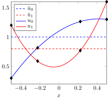
(a) Before limiting; notice the nonrealizable moments at the end points.

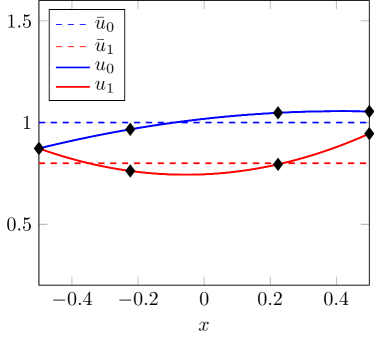
(b) After limiting; realizable.

Figure 1: Application of the realizability preserving limiter to the M₁ system for a quadratic polynomial. Here, $(u_{0},u_{1})$ are realizable only if $|u_{1}|<u_{0}$. Black squares indicate the spatial quadrature points $x_{q}$.

Since the full realizable set $\mathcal{R}_{\mathbf{b}}$ is characterized by the positive-definiteness of the associated Hankel matrices, computing the smallest $\theta$ such that $\mathbf{u}_{j}^{\theta}(t,x_{jq})\in\mathcal{R}_{\mathbf{b}}$ is in general difficult. Furthermore, for higher-dimensional problems (when dimension of the angular domain is more than one) the realizable set is in general not well-understood.

This computation is however easier for the numerically realizable set $\mathcal{R}_{\mathbf{b}}^{\mathcal{Q}}$ using its half-space representation. This representation is also intriguing because it extends to higher-dimensional problems, since even in these cases $\mathcal{R}_{\mathbf{b}}^{\mathcal{Q}}$ remains the interior of a cone generated by a convex polytope.

In the following for clarity of exposition we omit the time arguments and spatial-cell indices, therefore using $\bar{\mathbf{u}}$ to indicate the (always realizable) moment vector at the cell mean and $\mathbf{u}_{q}$ to indicate the (not necessarily realizable) moment vector at a quadrature point. In an implementation, the limiter is applied to every quadrature point in every cell.

To discuss the computation of $\theta$, first we assume that the moment vectors $\bar{\mathbf{u}}$ and $\mathbf{u}_{q}$ have been scaled such that $\max(\bar{u}_{0},u_{q0})=1/2$, where $\bar{u}_{0}$ and $u_{q0}$ are the zero-th components of $\bar{\mathbf{u}}$ and $\mathbf{u}_{q}$, respectively. Then the limited moment vector $\mathbf{u}_{q}^{\theta}:=\theta\bar{\mathbf{u}}+(1-\theta)\mathbf{u}_{q}$ satisfies $u^{\theta}_{q0}<1$ for all $\theta\in[0,1]$, and without loss of generality we can apply the limiter to move the moments into the bounded set

$$\left.\mathcal{R}_{\mathbf{b}}^{\mathcal{Q}}\right|_{u_{0}<1}=\left\{\mathbf{u}\in\mathcal{R}_{\mathbf{b}}^{\mathcal{Q}}~{}|~{}u_{0}<1\right\}.$$

instead of the full, unbounded set $\mathcal{R}_{\mathbf{b}}^{\mathcal{Q}}$. Now, using that $\mathcal{R}_{\mathbf{b}}^{\mathcal{Q}}$ is the cone generate by $\left.\mathcal{R}_{\mathbf{b}}^{\mathcal{Q}}\right|_{u_{0}=1}$ and Proposition 2.2, $\left.\mathcal{R}_{\mathbf{b}}^{\mathcal{Q}}\right|_{u_{0}<1}$ can be written as the interior of a convex polytope

$$\left.\mathcal{R}_{\mathbf{b}}^{\mathcal{Q}}\right|_{u_{0}<1}=\left\{\lambda\mathbf{u}:\lambda\in(0,1)\text{ and }\mathbf{u}\in\left.\mathcal{R}_{\mathbf{b}}^{\mathcal{Q}}\right|_{u_{0}=1}\right\}=\operatorname{int}\operatorname{co}\left\{0,\mathbf{b}(\mu_{1}),\mathbf{b}(\mu_{2}),\ldots,\mathbf{b}(\mu_{{n_{\mathcal{Q}}}})\right\}.$$

As a convex polytope, it has a half-space representation [4] of the form

$$\left.\mathcal{R}_{\mathbf{b}}^{\mathcal{Q}}\right|_{u_{0}<1}=\left\{\mathbf{u}\in\mathbb{R}^{N+1}:~{}\mathbf{a}_{i}^{T}\mathbf{u}<b_{i},i\in\{1,\ldots,d\}\right\},$$

where $d$ is the number of facets of the polytope. For each $i$-th facet, the vectors $\mathbf{a}_{i}$ and scalars $b_{i}$ are computed from the set of vertices defining the facet. These sets of vertices can be computed using standard convex-hull algorithms, and for our implementation we used the Matlab routine convhulln. These are fixed throughout the computation and therefore can be precomputed.

Candidate values $\theta_{qi}$ for the $\theta$ which ensures $\mathbf{u}_{q}^{\theta}\in\left.\mathcal{R}_{\mathbf{b}}^{\mathcal{Q}}\right|_{u_{0}<1}$ can now be computed for each $i$-th facet by

$$\mathbf{a}_{i}^{T}(\theta_{qi}\bar{\mathbf{u}}+(1-\theta_{qi})\mathbf{u}_{q})=b_{i}\quad\iff\quad\theta_{qi}=\frac{b_{i}-\mathbf{a}_{i}^{T}\mathbf{u}_{q}}{\mathbf{a}_{i}^{T}(\bar{\mathbf{u}}-\mathbf{u}_{q})}.$$

If we wanted to limit exactly to $\partial\mathcal{R}_{\mathbf{b}}^{\mathcal{Q}}$, we would first take

$$\theta_{q}^{\partial\mathcal{R}}:=\begin{cases}0&\text{if there is no }\theta_{qi}\in[0,1],\\ \max\{\theta_{qi}:\theta_{qi}\in[0,1]\}&\text{else;}\end{cases}$$

and then for the cell in question, we would apply the largest $\theta_{q}$ from the quadrature nodes: $\theta^{\partial\mathcal{R}}:=\max\{\theta_{q}^{\partial\mathcal{R}}\}$. This would ensure that the moment vectors at each quadrature node in the cell are in the realizable set or on its boundary.

In practice, however, we do not want to choose $\theta_{q}$ such that the limited moment vector $\theta_{q}\bar{\mathbf{u}}+(1-\theta_{q})\mathbf{u}_{q}$ lies exactly on the boundary of the realizable set $\partial\mathcal{R}_{\mathbf{b}}^{\mathcal{Q}}$, but rather so that the limited moment vector is in the interior of $\mathcal{R}_{\mathbf{b}}^{\mathcal{Q}}$. Therefore we define a tolerance $\varepsilon$ to add to each relevant $\theta_{qi}$ (that is in $[0,1]$) as well as those facets such that $\theta_{qi}\in[-\varepsilon,0]$, indicating that while $\mathbf{u}_{q}$ is on the correct side of the half space, it is closer than $\varepsilon$ to the facet. Keeping in mind that $\theta_{q}$ should not exceed one, this gives

$$\theta_{q}:=\begin{cases}0&\text{if there is no }\theta_{qi}\in[-\varepsilon,1],\\ \min\{1,\varepsilon+\max\{\theta_{qi}:\theta_{qi}\in[-\varepsilon,1]\}\}&\text{else.}\end{cases}$$

Finally, in the implemented version, for the cell we set $\theta=\max\{\theta_{q}\}$. Figure 2a shows an example for the full moment model with $N=2$.

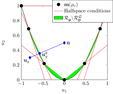
(a) Limiter example for $N=2$ full moments $\mathbf{p}$-basis with ${n_{\mathcal{Q}}}=7$ and, for simplicity of exposition, $u_{q0}=\bar{u}_{0}=1$.

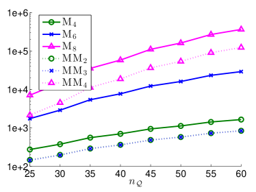
(b) The number of facets of $\mathcal{R}_{\mathbf{b}}^{\mathcal{Q}}$ for a few $\text{M}_{N}$ (for $N\in\{4,6,8\}$) and $\text{MM}_{N}$ (for $N\in\{2,3,4\}$) models. The number of facets of MM₂ and MM₃ are almost exactly the same.

Figure 2:

The main drawback to this implementation of the limiter is that, as illustrated in Figure 2b the number of facets $d$ grows rapidly both with the number of moments $N$ and the number of quadrature points ${Q}$. The numbers for this figure were computed using results from the study of convex polytopes, and a more detailed discussion is in the appendix. This issue was not a significant obstacle for our simulations but will be in higher dimensions where a much larger number of quadrature points is necessary. One clear speed up is that not every $\theta_{qi}$ should be computed, as many facets do not intersect the line between $\bar{\mathbf{u}}$ and $\mathbf{u}_{q}$. More importantly, however, an implementation in higher-dimensions will probably have to further approximate $\mathcal{R}_{\mathbf{b}}^{\mathcal{Q}}$ by removing some irrelevant facets.

Remark 3.4.

There is actually no loss in accuracy by limiting to $\mathcal{R}_{\mathbf{b}}^{\mathcal{Q}}$ instead of $\mathcal{R}_{\mathbf{b}}$ when the quadrature $\mathcal{Q}$ defining $\mathcal{R}_{\mathbf{b}}^{\mathcal{Q}}$ is the same as the quadrature used to compute all angular integrals: In this case we are solving the moment equations (2.4) with quadrature approximations to the angular integrals, and the numerical solution indeed lives on $\mathcal{R}_{\mathbf{b}}^{\mathcal{Q}}$. (Furthermore, the function $\mathbf{f}$ can only be evaluated on $\mathcal{R}_{\mathbf{b}}^{\mathcal{Q}}$.) The numerical solutions using quadrature then converge to moment equations with exact integrals as the quadrature rule converges.

3.5 Slope limiting

Although the realizability limiter plays some role in dampening spurious oscillations in numerical solutions, further dampening is needed [23]. We use the standard TVBM corrected minmod limiter proposed in [6].

Assuming that the major part of the spurious oscillations are generated in the linear part of the underlying polynomial, whose slope in the $j$-th cell is simply $\hat{\mathbf{u}}_{j}^{1}$, a basic limiter can be defined as

$$\Lambda^{\text{scalar}}_{j}(\hat{\mathbf{u}})=\left\{\begin{array}[]{cc}\left(\begin{array}[]{c}\left(\hat{\mathbf{u}}^{0}_{j}\right)^{T}\\ \left(D_{j}(\hat{\mathbf{u}})\right)^{T}\\ (0,0,\ldots,0)\end{array}\right)&\text{ if }\begin{array}[]{c}\left|\hat{\mathbf{u}}_{j}^{1}\right|\geq M(\Delta x_{j})^{2}\text{ and,}\\ D_{j}(\hat{\mathbf{u}})\neq\hat{\mathbf{u}}_{j}^{1}\end{array}\\ \hat{\mathbf{u}}_{j}&\text{otherwise}\end{array}\right.$$

for the $j$-th cell and the case $k=2$, that is piecewise quadratic approximations, so that the final row of zeros in the first case indicates that the coefficients for the quadratic basis functions are set to zero for each moment component. The absolute value and inequality are applied component-wise, and

$$D_{j}(\hat{\mathbf{u}})=D(\hat{\mathbf{u}}_{j-1},\hat{\mathbf{u}}_{j},\hat{\mathbf{u}}_{j+1}):=m(\hat{\mathbf{u}}_{j}^{1},\hat{\mathbf{u}}_{j+1}^{0}-\hat{\mathbf{u}}_{j}^{0},\hat{\mathbf{u}}_{j}^{0}-\hat{\mathbf{u}}_{j-1}^{0}).$$

The label “scalar” is used because the limiter is directly applied to each scalar component of $\mathbf{u}_{h}$. The function $m$ is the standard minmod function applied component-wise:

$$m(a_{1},a_{2},a_{3}) =\begin{cases}\operatorname{sign}(a_{1})\min\{|a_{1}|,|a_{2}|,|a_{3}|\}&\text{if }\operatorname{sign}(a_{1})=\operatorname{sign}(a_{2})=\operatorname{sign}(a_{3}),\\ 0&\text{else}.\end{cases}$$

The constant $M$ is a problem-dependent estimate of the second derivative, though we note that in [6] the authors did not find the solutions very sensitive to the value chosen for this parameter.

However, it has been found that applying the limiter to the components themselves may introduce non-physical oscillations around an otherwise monotonic solution [5]. Therefore we instead apply the limiter to the local characteristic fields of the solution. The characteristic fields are found by transforming the moment vector $\mathbf{u}$ using the matrix $\mathbf{V}_{j}$, whose columns hold the eigenvectors of the Jacobian $\partial\mathbf{f}/\partial\mathbf{u}$ evaluated at the cell mean $\bar{\mathbf{u}}_{j}$. We then transform back to the moment variables after applying the limiter. In the end, since $\hat{\mathbf{u}}_{j}$ is a matrix of size $(k+1)\times(N+1)$, this transformation is accomplished by post-multiplying with $\mathbf{V}_{j}^{-T}$ so that

$$\Lambda_{j}(\hat{\mathbf{u}})=\Lambda^{\text{scalar}}_{j}(\hat{\mathbf{u}}\mathbf{V}_{j}^{-T})\mathbf{V}_{j}^{T},$$

where $\hat{\mathbf{u}}\mathbf{V}^{-T}_{j}$ is understood as $(\ldots,\hat{\mathbf{u}}_{j-1}\mathbf{V}^{-T}_{j},\hat{\mathbf{u}}_{j}\mathbf{V}^{-T}_{j},\hat{\mathbf{u}}_{j+1}\mathbf{V}^{-T}_{j},\ldots)$. We apply this limiter to every Runge-Kutta stage.

The Jacobian is computed at the cell means $\bar{\mathbf{u}}_{j}$ using (3.4). This indeed also implies that we must solve the dual problem (2.6) to compute $\hat{\boldsymbol{\alpha}}(\bar{\mathbf{u}}_{j})$ for each cell. For cases when the matrix $\mathbf{V}_{j}$ has a condition number (defined using the two-norm) greater than a tolerance $\kappa_{\text{jac}}$, we apply the scalar limiter.

There are more advanced limiter strategies, for example WENO limiting [25, 38] or generalized minmod-limiting [16], removing the drawback of having a problem-dependent parameter $M$. The slope limiter is however not a focus of this work.

4 Numerical results

We used the following parameter values:

$\tau$	=	$10^{-9}$	Optimization gradient tolerance,
$\{r_{m}\}$	=	$\{0,10^{-8},10^{-6},10^{-4},10^{-3}\}$	Outer regularization loop in optimizer,
$k_{r}$	=	$50$	Number of optimization iterations before
			advancing outer regularization loop,
${n_{\mathcal{Q}}}$	=	$40$	Number of angular quadrature points,
$M$	=	$50$	Slope-limiter constant, value suggested
			in [6],
$\varepsilon$	=	$10^{-14}$	Realizability limiter tolerance,
$\kappa_{\text{jac}}$	=	$10^{5}$	Condition-number tolerance for applying the characteristic
			transformation in the slope limiter.

For the angular quadrature we used $({n_{\mathcal{Q}}}/2)$-point Gauss-Lobatto rules over both $\mu\in[-1,0]$ and $\mu\in[0,1]$. At the first time step, the initial multipliers for the optimizer (recall Section 3.3) are those of the isotropic density with the appropriate zeroth-order moment. For the rest of the simulation, the initial multipliers are those from the same point in space at the previous time step.

To set the time step we use condition (3.13) with equality.

4.1 Convergence tests

We numerically test the convergence of the scheme two ways: First, we use the method of manufactured solutions on the total scheme, and second we focus on the convergence of the spatial reconstructions using the realizability limiter near the boundary of realizability.

4.1.1 Manufactured solution

In general, analytical solutions for minimum-entropy models are not known. Therefore, to test the convergence and efficiency of our scheme, we use the method of manufactured solutions. To avoid the effects of the boundary we use periodic boundary conditions, and we set the spatial domain to $X=(-\pi,\pi)$.

We begin by defining a kinetic density in the form of the entropy ansatz and which is periodic in space for every $t$:

$$\phi(t,x,\mu)= \exp(\alpha_{0}(t,x)+\alpha_{1}(t,x)\mu),$$ (4.1a)

$$\alpha_{0}(t,x)= -K-\sin(x-t)+c_{0}t-c_{1},$$ (4.1b)

$$\alpha_{1}(t,x)= K+\sin(x-t).$$ (4.1c)

A source term is defined by applying the transport operator to $\phi$:

$$S(t,x,\mu):=\partial_{t}\phi(t,x,\mu)+\mu\partial_{x}\phi(t,x,\mu).$$

Thus by inserting this $S$ into (2.1) (and taking $\sigma_{\mathrm{a}}=\sigma_{\mathrm{s}}=0$) we have that $\phi$ is, by construction, a solution of (2.1).

A tedious but straightforward computation shows that choosing $c_{0}=4$ gives $S\geq 0$, which means that Theorem 3.3 will apply to the resulting moment system (for any $K$). Furthermore we take

$$c_{1} =c_{0}t_{\rm f}-K+1-\log\left(\cfrac{K-1}{2\sinh(K-1)}\right)$$

so that the maximum value of $\langle\phi\rangle$ for $(t,x)\in[0,t_{\rm f}]\times X$ is one. The parameter $K$ can be increased to make $\phi$ look increasingly like a Dirac delta at $\mu=1$.

Since our solution has the form of an entropy ansatz, $\mathbf{v}=\langle\mathbf{b}\phi\rangle$ is also a solution of (2.4) whenever $1$ and $\mu$ are in the linear span of the basis functions $\mathbf{b}$. Clearly this holds for the M_N and MM_N models for $N\geq 1$. Notice also that $\mathbf{v}$ approaches the boundary of realizability as $K$ is increased.

We used the final time $t_{\rm f}=\pi/5$ and chose $K=55$, for which the maximum value of $u_{1}/u_{0}$ is about $0.98$ (recall that $|u_{1}/u_{0}|<1$ is necessary for realizability). In the following, we used the M₃ model so that our results included the effects of the numerical optimization.

We compute errors in the zero-th moment of the solution, which we denote $v_{0}(t,x)=\langle\phi(t,x,\cdot)\rangle$. Then $L^{1}$ and $L^{\infty}$ errors for the zero-th moment $u_{0,h}(t,x)$ (that is, the zero-th component of a numerical solution $\mathbf{u}_{h}$) are defined as

$$E^{1}_{h}=\int_{X}\left|v_{0}(t_{\rm f},x)-u_{0,h}(t_{\rm f},x)\right|dx\quad\mbox{and}\quad E^{\infty}_{h}=\max_{x\in X}\left|v_{0}(t_{\rm f},x)-u_{0,h}(t_{\rm f},x)\right|,$$ (4.2)

respectively. We approximate the integral in $E^{1}_{h}$ using a 100-point Gauss-Lobatto quadrature rule over each spatial cell $I_{j}$, and $E^{\infty}_{h}$ is approximated by taking the maximum over these quadrature nodes. The observed convergence order $\nu$ is defined by

$$\frac{E^{p}_{h1}}{E^{p}_{h2}}=\left(\frac{\Delta x_{1}}{\Delta x_{2}}\right)^{\nu}$$ (4.3)

where for $i\in\{1,2\}$, $E^{p}_{hi}$ is the error $E^{p}_{h}$ for the numerical solution using cell size $\Delta x_{i}$, for $p\in\{1,\infty\}$.

A convergence table is presented in Table 1 using a tight gradient tolerance in the optimization of $\tau=10^{-11}$. We observe that the expected convergence rates are achieved both in $L^{1}$- and $L^{\infty}$-errors, although for $k=0$, the solution has only just begun to reach the convergent regime. In Figure 3a we plot the $L^{\infty}$-error versus the computation time for the solution for the same value of $\tau$. Here we clearly see that higher-order methods are more efficient.

The scheme is not convergent for arbitrarily large values of $K$. For large values of $K$, the numerical solution will veer so close to the boundary of the realizable set that the optimization will have to use regularization, thus introducing errors into the solution. This was observed in [1], though here we can display this effect more precisely. In Figure 3b, we show the results using $K=110$ for three spatial discretizations. In the most coarse discretization (${J}=40$), regularization is never necessary, but after doubling the number of cells, a few regularizations are used and their effects can be seen in the figure. Here, the optimizer regularizes four problems with $r=10^{-8}$, around $x=-1.76,\,-1.68,\,0.51,\,0.74$ at $t=0.38,\,0.44,\,0.35,\,0.52$, respectively, and the effect on the error spreads, mostly (to the right, the propagation direction of the solution), and magnifies slightly until the final time. The observed convergence order for $E^{1}_{h}$ from ${J}=40$ to $80$ is $\nu=2.9$ while the corresponding $E_{h}^{\infty}$ order is $\nu=2.1$. When doubling the number of cells again (up to ${J}=160$), the optimizer must regularize now only three problems with $r=10^{-8}$, this time around $x=-1.74,\,-1.66,\,1.04$ at $t=0.56,\,0.51,\,0.44$, respectively. Indeed, immediately from the figure one can see that convergence in the $E^{\infty}_{h}$ error has stopped and the observed convergence rate in $E^{1}_{h}$ from ${J}=80$ to $160$ is only $\nu=1.6$.

	$k=0$			$k=1$			$k=2$
${J}$	$E^{1}_{h}$		$\nu$	$E^{1}_{h}$		$\nu$	$E^{1}_{h}$		$\nu$
20	4.	087e+00	—	3.	524e-02	—	1.	897e-05	—
40	2.	608e+00	0.6	9.	532e-03	1.9	2.	416e-06	3.0
80	1.	507e+00	0.8	2.	482e-03	1.9	3.	049e-07	3.0
160	8.	161e-01	0.9	6.	333e-04	2.0	3.	828e-08	3.0
320	4.	256e-01	0.9	1.	600e-04	2.0	4.	796e-09	3.0
640	2.	174e-01	1.0	4.	020e-05	2.0	6.	072e-10	3.0
	$E^{\infty}_{h}$		$\nu$	$E^{\infty}_{h}$		$\nu$	$E^{\infty}_{h}$		$\nu$
20	3.	339e-01	—	3.	164e-03	—	9.	283e-06	—
40	2.	129e-01	0.6	8.	543e-04	1.9	1.	241e-06	2.9
80	1.	230e-01	0.8	2.	222e-04	1.9	1.	609e-07	2.9
160	6.	662e-02	0.9	5.	666e-05	2.0	2.	048e-08	3.0
320	3.	474e-02	0.9	1.	431e-05	2.0	2.	589e-09	3.0
640	1.	775e-02	1.0	3.	595e-06	2.0	3.	365e-10	2.9

Table 1: $L^{1}$- and $L^{\infty}$-errors and observed convergence order $\nu$ for the manufactured solution (4.1) with optimization gradient tolerance $\tau=10^{-11}$.

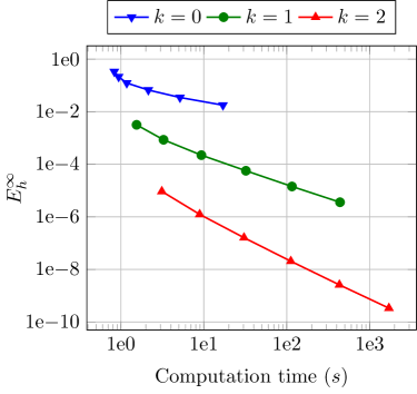
(a) $L^{\infty}$-Efficiency, $\tau=10^{-11}$. Here we used the same numbers of cells as in Table 1.

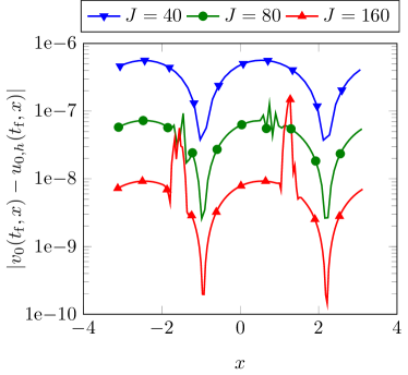
(b) Regularization destroying convergence for $K=110$.

Figure 3: Using the manufactured solution to consider the efficiency of higher-order methods and the effects of regularization.

4.1.2 Convergence of the limited spatial reconstructions

Despite choosing a manufactured solution which lies close to the boundary of realizability, the realizability limiter was never active in any of our simulations in Section 4.1.1. Therefore in this section we artificially define a curve of moment vectors in space, reconstruct this curve in the finite-element space $V_{h}^{2}$ of discontinuous quadratic polynomials (recall (3.2)), and apply the limiter to move the reconstruction back into the set of numerically realizable moments. We then measure the convergence of this limited reconstruction.

For simplicity, we only consider the monomial basis $\mathbf{b}=\mathbf{p}$. Using the Dirac delta function $\delta=\delta(\mu)$, we first choose two moment vectors $\mathbf{u}_{0}$ and $\mathbf{u}_{1}$ which lie arbitrarily close to the boundary of the numerically realizable set:

$$\mathbf{u}_{0} :=(1-\gamma)\left\langle\mathbf{p}\delta(\mu-\mu_{0})\right\rangle+\gamma\mathbf{u}_{\text{iso}}=(1-\gamma)\mathbf{p}(\mu_{0})+\gamma\mathbf{u}_{\text{iso}}$$

$$\mathbf{u}_{1} :=10^{-8}\left((1-\gamma)\left\langle\mathbf{p}\delta(\mu+1)\right\rangle+\gamma\mathbf{u}_{\text{iso}}\right)=10^{-8}\left((1-\gamma)\mathbf{p}(-1)+\gamma\mathbf{u}_{\text{iso}}\right)$$

where $\mu_{0}\approx 0.5403$, which is a node from the angular quadrature we use (see the beginning of Section 4), $\mathbf{u}_{\text{iso}}$ are the moments of the isotropic density (see (3.9)), and $\gamma\in[0,1]$ controls the distance to the boundary. For $N>1$, both $\mathbf{u}_{0}$ and $\mathbf{u}_{1}$ lie on the boundary of the realizable set when $\gamma=0$. Since the Dirac delta functions are placed at nodes in the angular quadrature, $\mathbf{u}_{0}$ and $\mathbf{u}_{1}$ (and any convex combination thereof) are in $\mathcal{R}_{\mathbf{p}}^{\mathcal{Q}}$ for $\gamma\in(0,1]$, and so we define a curve of moments in space by taking convex combinations of $\mathbf{u}_{0}$ and $\mathbf{u}_{1}$:

$$\mathbf{u}(x):=(1-\lambda(x))\mathbf{u}_{0}+\lambda(x)\mathbf{u}_{1},\quad x\in[-1,1],$$ (4.4)

where $\lambda(x)\in[0,1]$ is given by

$$\lambda(x):=\frac{\cos(\pi x)+1}{2},\quad x\in[-1,1].$$

To perform the convergence test, we project $\mathbf{u}(x)$ onto $V_{h}^{2}$ for increasing numbers of cells ${J}$ and then apply the realizability limiter. Errors and observed convergence order are computed as in (4.2) and (4.3), respectively, over the finest grid of the tests, here ${J}=512$ cells.

We found that taking $\gamma\in[10^{-10},10^{-2}]$ places the moment curve $\mathbf{u}(x)$ close enough to the boundary of realizability that the realizability limiter was active for every number of cells we considered. In Table 2 we show convergence rates for the smallest $\gamma$ in this range. These results show the desired third-order convergence. In this table we include the column $\theta_{\max}$, which gives the maximum value of $\theta$ from the realizability limiter over all spatial cells. That $\theta_{\max}$ is nonzero in each row indicates that the realizability limiter was active for every reconstruction. We observed similar results for every moment component and moment curves of any order $N\in\{2,3,4,5\}$.

	$u_{0}$						$u_{1}$
${J}$	$E^{1}_{h}$		$\nu$	$E^{\infty}_{h}$		$\nu$	$E^{1}_{h}$		$\nu$	$E^{\infty}_{h}$		$\nu$	$\theta_{\max}$
8	1.	072e-03	—	1.	848e-03	—	5.	790e-04	—	9.	983e-04	—	1.	56e-02
16	1.	130e-04	3.2	2.	469e-04	2.9	6.	108e-05	3.2	1.	334e-04	2.9	4.	27e-03
32	1.	342e-05	3.1	3.	137e-05	3.0	7.	253e-06	3.1	1.	695e-05	3.0	1.	39e-03
64	1.	655e-06	3.0	3.	937e-06	3.0	8.	943e-07	3.0	2.	127e-06	3.0	6.	61e-04
128	2.	060e-07	3.0	4.	927e-07	3.0	1.	113e-07	3.0	2.	662e-07	3.0	4.	48e-04
256	2.	564e-08	3.0	6.	160e-08	3.0	1.	385e-08	3.0	3.	328e-08	3.0	2.	51e-04
512	3.	188e-09	3.0	7.	700e-09	3.0	1.	723e-09	3.0	4.	160e-09	3.0	3.	76e-06

Table 2: $L^{1}$- and $L^{\infty}$-errors and observed convergence order $\nu$ for the first two components of the realizability-limited, piecewise quadratic reconstruction of $\mathbf{u}(x)$ from (4.4) with $\gamma=10^{-10}$ and moment order $N=4$.

However, it has been remarked in [36] that in some pathological situations this limiter may reduce accuracy to second order. We can demonstrate this by pushing $\mathbf{u}(x)$ closer to the boundary of realizability by setting $\gamma=10^{-11}$. These results are given in Table 3, where in the $L^{1}$ error we still see third-order convergence, but in the $L^{\infty}$ error the convergence has degraded to second order.

In further tests, which for brevity we omit here, we observed similar behavior as we decrease $\gamma$ until we arrive at $10^{-14}$, which is the value of the tolerance in the realizability limiter (see the beginning of Section 4). At this point convergence is only first order as expected.

	$u_{0}$						$u_{1}$
${J}$	$E^{1}_{h}$		$\nu$	$E^{\infty}_{h}$		$\nu$	$E^{1}_{h}$		$\nu$	$E^{\infty}_{h}$		$\nu$	$\theta_{\max}$
8	1.	308e-03	—	1.	848e-03	—	7.	066e-04	—	9.	983e-04	—	1.	93e-02
16	1.	224e-04	3.4	2.	469e-04	2.9	6.	614e-05	3.4	1.	334e-04	2.9	8.	11e-03
32	1.	460e-05	3.1	3.	137e-05	3.0	7.	889e-06	3.1	1.	695e-05	3.0	5.	23e-03
64	1.	805e-06	3.0	7.	105e-06	2.1	9.	754e-07	3.0	3.	839e-06	2.1	4.	55e-03
128	2.	247e-07	3.0	1.	721e-06	2.0	1.	214e-07	3.0	9.	299e-07	2.0	4.	32e-03
256	2.	799e-08	3.0	4.	162e-07	2.0	1.	512e-08	3.0	2.	248e-07	2.0	4.	15e-03
512	3.	457e-09	3.0	8.	958e-08	2.2	1.	868e-09	3.0	4.	840e-08	2.2	3.	57e-03

Table 3: $L^{1}$- and $L^{\infty}$-errors and observed convergence order $\nu$ for the first two components of the realizability-limited, piecewise quadratic reconstruction of $\mathbf{u}(x)$ from (4.4) with $\gamma=10^{-11}$ and moment order $N=4$.

That the limiter works so close to the boundary of realizability is satisfactory to us: When moment vectors as close as $10^{-10}$ to the boundary of realizability appear in a simulation, errors from the numerical optimization are likely to affect convergence before these effects of the realizability limiter play a role.

4.2 Plane source

In this test case we start with an isotropic distribution where the initial mass is concentrated in the middle of an infinite domain $x\in(-\infty,\infty)$:

$$\psi_{t=0}(x,\mu)=\psi_{\rm floor}+\delta(x)$$

where the small parameter $\psi_{\rm floor}=0.5\times 10^{-8}$ is used to model a vacuum. In practice, a bounded domain must be used, so we choose a domain large enough that the boundary should have only negligible effects on the solution: thus for our final time $t_{\rm f}=1$, we take $X=[x_{\text{L}},x_{\text{R}}]=[-1.2,1.2]$. At the boundary we set

$$\psi_{\text{L}}(t,\mu)\equiv\psi_{\rm floor}\quad\mbox{and}\quad\psi_{\text{R}}(t,\mu)\equiv\psi_{\rm floor}$$

We use isotropic scattering and no absorption, therefore $\mathcal{C}\left(\psi\right)=\frac{1}{2}\langle\psi\rangle-\psi$, $\sigma_{\mathrm{s}}=1$ and $\sigma_{\mathrm{a}}=0$.

We approximate the delta function by using an even number of spatial cells and splitting the delta into the cells immediately to the left and right of $x=0$. This is then projected into $V_{h}^{k}$ using (3.3b). All solutions here are computed with ${J}=300$ cells and spatial polynomials of degree $k=2$.

Figure 4 presents solutions for different moment models. This figure includes a reference solution, which we computed using our scheme for the P₉₉ model with ${J}=2000$ cells and spatial order $k=0$. The oscillations we see have been observed before and arise due to the fact that we are using moment models (which are indeed spectral methods) on a non-smooth problem. Indeed, our M_N results agree well with those in [12]. The full- and mixed-moment models look largely similar for the same numbers of degrees of freedom, with the notable differences being around $x=0$. Here the mixed-moment solutions are much more sharply peaked while the full-moment solutions are more flat and wider. The discrepancy in magnitude, however, seems to decrease as $N$ increases, which agrees with the expectation that both methods are converging as $N\to\infty$.

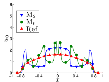
(a) Full-moment models.

(b) Mixed-moment models.

Figure 4: Local density $u_{0}$ for different models and a reference solution at $t=0.8$ in the plane-source problem.

Figure 5 shows the activity of the realizability limiter. The realizability limiter is most active along the fronts where particles from the initial impulse are first entering the domain, which is as expected, because this is where the moment vectors of the solution lie closest to the boundary of realizability [2]. We also see that as the number of moments increases, the activity of the realizability limiter increases as well. This is also not surprising, since realizability conditions typically require tighter and tighter bounds on the moment components as their order increases. Thus numerical errors of a similar size will have an increasingly large chance of pushing the solution out of the realizable set. We did not observe significant differences between the full-moment and mixed-moment models.

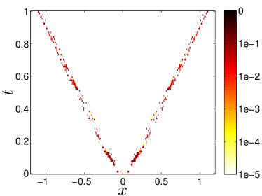
(a) M₃

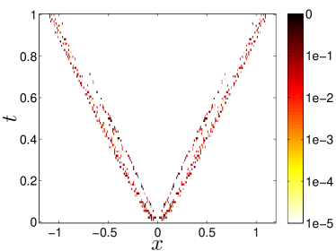
(b) M₅

Figure 5: The value of $\theta$ in the realizability limiter for two models of the plane-source problem. Note that we choose a logarithmic scale so that even small values of $\theta$ are noticeable.

4.3 Two beams

This test case models two beams entering a (nearly) empty absorbing medium. This is a classical test problem used to illustrate the shortcomings of the M₁ model, whose steady-state solution for this problem has a nonphysical shock. This test case is also challenging for the numerical optimization [2].

The domain is $X=(-0.5,0.5)$, and the beams are specified by boundary conditions

$$\psi_{\text{L}}(t,\mu)=\frac{1}{\Sigma}\exp\left(-\frac{(\mu-1)^{2}}{2\Sigma^{2}}\right)\quad\mbox{and}\quad\psi_{\text{R}}(t,\mu)=\frac{1}{\Sigma}\exp\left(-\frac{(\mu+1)^{2}}{2\Sigma^{2}}\right),$$

with $\Sigma=50$. The initial condition again approximates a vacuum similarly as before:

$$\psi(0,x,\mu)=\psi_{\rm floor}=0.5\times 10^{-8}.$$

Finally, we use absorption parameter $\sigma_{a}=2$ and no scattering, $\sigma_{s}=0$. Again, all solutions here are computed with ${J}=300$ cells and spatial polynomials of degree $k=2$.

Our numerical solutions for the local density $u_{0}$ all look qualitatively the same—with the notable exception of the M₁ model—and match the true steady-state solution, so in Figure 6a we only present one example solution for the unfamiliar reader. We do note, however, that our steady-state solutions for the full-moment models do not contain the shocks observed in [12]. This difference is apparently due to the fact that we use sharply forward-peaked boundary conditions, where as isotropic boundary conditions were used in [12]. As shown in Figure 6a, the mixed-moment solutions do not appear to contain any steady-state shocks either.

In Figure 6b we present a zoomed-in view of the oscillations present in a typical transient solution. These oscillations become more noticeable for higher-order models (M_N for $N\geq 4$ and MM_N for $N\geq 3$). It seems clear to us that these are numerical artifacts, and we believe they would be mitigated with a more sophisticated slope limiter.

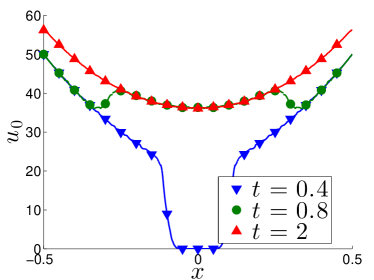
(a) MM₂

(b) The M₄ model at $t=0.8$.

Figure 6: Local density $u_{0}$ for different models at $t=0.8$ in the two-beam problem.

The activity of the realizability limiter again increases with the number of moments, but in this problem we see differences between full- and mixed-moment models. Figure 7 illustrates this difference. The reason for this difference is not yet clear to us, but it seems to indicate that the mixed-moment model is converging more slowly to steady state.

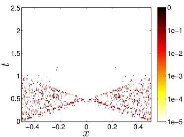
(a) M₄

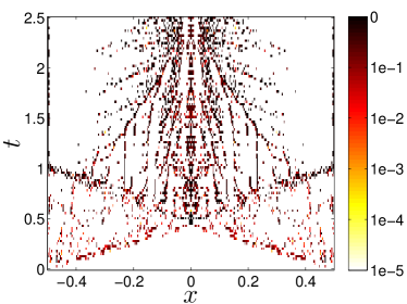
(b) MM₂

Figure 7: The value of $\theta$ in the realizability limiter for two models of the two-beam problem. Note that we choose a logarithmic scale so that even small values of $\theta$ are noticeable.

5 Conclusions and outlook

We presented a high-order Runge-Kutta discontinuous Galerkin scheme for minimum-entropy moment models of linear kinetic equations in one space dimension. The key issue for higher-order methods for minimum-entropy moment models is that the numerical solution typically leaves the set of realizable moments, even though standard techniques can be used to show that the cell means of the solution remain realizable. We address this problem using a realizability limiter inspired by the positivity-preserving limiter used in [35] for the Euler equations. Such a limiter requires the computation of the intersection of a line in moment space with the boundary of the realizable set, a set which typically has nonlinear boundaries. We are able to approximate this intersection by replacing the true realizable set with its quadrature-based approximation, which is a convex polytope. This quadrature-based approximation is intriguing because it is a convex polytope for any moment order and any dimension of the angular domain indicating that our techniques could be extended to these cases.

We constructed a new manufactured solution whose source term is realizable, thus allowing us to consider target solutions closer to the boundary of the realizable set. These tests show that our scheme converges as expected and that higher-order schemes are more efficient. We also present numerical solutions for standard benchmark problems, where we are able to compare full- and mixed-moment models.

Future work should focus on a parallelized implementation for two- and three-dimensional problems. Theoretically, implementation of the quadrature-based realizability limiter requires no change because the convex polytopic structure of $\mathcal{R}_{\mathbf{b}}^{\mathcal{Q}}$ holds in any dimension. Practically speaking, however the main challenge is that the number of facets grows quickly with the number of moments and number of quadrature points, both of which will be higher. Further work in higher-order methods will also have to consider new methods for time integration, as here we relied heavily on the SSP property, which is not possible past fourth-order. Relatedly, at least partially implicit time integrators should be investigated, particularly in the context of constructing an asymptotic preserving numerical method for the moment system.

Appendix A The number of facets in $\left.\mathcal{R}_{\mathbf{p}}^{\mathcal{Q}}\right|_{u_{0}=1}$ and $\left.\mathcal{R}_{\mathbf{m}}^{\mathcal{Q}}\right|_{u_{0}=1}$

Even with some speed-ups in the computation of the facet-intersections and possibly approximations by removing facets, the number of facets plays a large role in determining the complexity of finding the intersection of a ray with the boundary of the convex polytope $\left.\mathcal{R}_{\mathbf{b}}^{\mathcal{Q}}\right|_{u_{0}<1}$. In this section we mention how some results from the study of convex polytopes give the exact number of facets in the full-moment case, and then we compare this with an upper bound of the number of facets in the mixed-moment case.

First, some notational remarks for this section: For convenience, we work with the closures $\overline{\mathcal{R}_{\mathbf{b}}^{\mathcal{Q}}}|_{u_{0}\leq 1}$ and $\overline{\mathcal{R}_{\mathbf{b}}^{\mathcal{Q}}}|_{u_{0}=1}$ of $\left.\mathcal{R}_{\mathbf{b}}^{\mathcal{Q}}\right|_{u_{0}<1}$ and $\left.\mathcal{R}_{\mathbf{b}}^{\mathcal{Q}}\right|_{u_{0}=1}$ respectively. When working with $\overline{\mathcal{R}_{\mathbf{b}}^{\mathcal{Q}}}|_{u_{0}=1}$, we consider it as a subset of $\mathbb{R}^{N}$ (or $\mathbb{R}^{2N}$ in the mixed-moment case), and use the notation $\mathbf{u}_{1}$ and $\mathbf{b}_{1}$ to indicate the final $N$ (or $2N$) entries of $\mathbf{u}$ and $\mathbf{b}$ respectively. We also often work with the matrix form of the half-space representation, so for example $\overline{\mathcal{R}_{\mathbf{b}}^{\mathcal{Q}}}|_{u_{0}=1}=\{\mathbf{u}_{1}:A\mathbf{u}_{1}\leq b\}$, for a matrix $A\in\mathbb{R}^{d\times N}$ with rows $\{\mathbf{a}^{T}_{i}\}_{i=1}^{d}$ and a vector $b\in\mathbb{R}^{d}$. Finally, we omit proofs in this section because we consider the arguments needed to be unenlightening and relatively straightforward.

We first note that the number of facets of $\overline{\mathcal{R}_{\mathbf{b}}^{\mathcal{Q}}}|_{u_{0}\leq 1}$ is only one more than that of $\overline{\mathcal{R}_{\mathbf{b}}^{\mathcal{Q}}}|_{u_{0}=1}$:

Proposition A.1.

If $A$ and $b$ define a half-space representation of $\overline{\mathcal{R}_{\mathbf{b}}^{\mathcal{Q}}}|_{u_{0}=1}$, then a half-space representation of $\overline{\mathcal{R}_{\mathbf{b}}^{\mathcal{Q}}}|_{u_{0}\leq 1}$ is:

$$\left.\overline{\mathcal{R}_{\mathbf{b}}^{\mathcal{Q}}}\right|_{u_{0}\leq 1}=\left\{\mathbf{u}=\begin{pmatrix}u_{0}\\ \mathbf{u}_{1}\end{pmatrix}:\begin{pmatrix}1&0\\ -b&A\end{pmatrix}\begin{pmatrix}u_{0}\\ \mathbf{u}_{1}\end{pmatrix}\leq\begin{pmatrix}1\\ 0\end{pmatrix}\right\}.$$

Therefore in the sequel we focus on the number of facets of $\overline{\mathcal{R}_{\mathbf{b}}^{\mathcal{Q}}}|_{u_{0}=1}$.

First we consider the full-moment case. The convex polytope $\overline{\mathcal{R}_{\mathbf{p}}^{\mathcal{Q}}}|_{u_{0}=1}\subset\mathbb{R}^{N}$ is known as the cyclic polytope and plays a special role in the study of convex polytopes. The Upper Bound Theorem states that for a given number of vertices in a given dimension, the cyclic polytope has the maximum number of facets [4]. Gale’s evenness condition or the Dehn-Sommerville equations can be used to show that the number of facets is

$$C(N,{n_{\mathcal{Q}}})=\begin{pmatrix}{n_{\mathcal{Q}}}-\left\lfloor\frac{1}{2}(N+1)\right\rfloor\\ {n_{\mathcal{Q}}}-N\end{pmatrix}+\begin{pmatrix}{n_{\mathcal{Q}}}-\left\lfloor\frac{1}{2}(N+2)\right\rfloor\\ {n_{\mathcal{Q}}}-N\end{pmatrix}$$

for ${n_{\mathcal{Q}}}>N>1$ [4], where $\left\lfloor\cdot\right\rfloor$ indicates the integer part of its argument. We note that this holds for any choice of distinct quadrature nodes $\{\mu_{i}\}$. Since $\overline{\mathcal{R}_{\mathbf{p}}^{\mathcal{Q}}}|_{u_{0}=1}$ has $C(N,{n_{\mathcal{Q}}})$ facets, there exists a half-space representation such that $A\in\mathbb{R}^{C(N,{n_{\mathcal{Q}}})\times N}$ and $b\in\mathbb{R}^{C(N,{n_{\mathcal{Q}}})}$. Unpacking the definition of the binomial coefficient we can see that for fixed, even $N$, we have $C(N,{n_{\mathcal{Q}}})=\mathcal{O}({n_{\mathcal{Q}}}^{N/2})$, and for fixed, odd $N$ we have $C(N,{n_{\mathcal{Q}}})=\mathcal{O}({n_{\mathcal{Q}}}^{(N-1)/2})$.

One can see from Figure 2b that $\text{MM}_{N}$ models appear always to have fewer facets than the corresponding $\text{M}_{N}$ models. To show that this holds more generally, we first need a half-space representation for $\overline{\mathcal{R}_{\mathbf{m}}^{\mathcal{Q}}}|_{u_{0}=1}$. This representation can be derived using the half-space representations from the full-moment case.

Proposition A.2.

Let $A_{\pm}$ and $b_{\pm}$ define half-space representations for the convex polytopes formed by the basis functions on the positive and negative subintervals respectively:

$$\operatorname{co}\left\{\mathbf{p}_{1}(\mu_{i})\right\}_{\mu_{i}\geq 0} =\left\{\mathbf{u}_{1+}:A_{+}\mathbf{u}_{1+}\leq b_{+}\right\},$$

$$\operatorname{co}\left\{\mathbf{p}_{1}(\mu_{i})\right\}_{\mu_{i}\leq 0} =\left\{\mathbf{u}_{1-}:A_{-}\mathbf{u}_{1-}\leq b_{-}\right\}.$$

We assume $b_{\pm}\geq 0$ component-wise. Then a half-space representation for $\overline{\mathcal{R}_{\mathbf{m}}^{\mathcal{Q}}}|_{u_{0}=1}$ is given by

$$\left.\overline{\mathcal{R}_{\mathbf{m}}^{\mathcal{Q}}}\right|_{u_{0}=1}=\left\{\mathbf{u}_{1}=\begin{pmatrix}\mathbf{u}_{1+}\\ \mathbf{u}_{1-}\end{pmatrix}:A\mathbf{u}_{1}\leq b\right\},$$

where

$$A=\begin{pmatrix}A_{+}&0\\ 0&A_{-}\\ \vdots&\vdots\\ b^{-1}_{+i}\mathbf{a}_{+i}^{T}&b^{-1}_{-j}\mathbf{a}_{-j}^{T}\\ \vdots&\vdots\end{pmatrix}\quad\mbox{and}\quad b=\begin{pmatrix}b_{+}\\ b_{-}\\ \vdots\\ 1\\ \vdots\end{pmatrix};$$

where the last rows of the $A$ include only those pairs $\{i,j\}$ such that neither $b_{+i}$ nor $b_{-j}$ is equal to zero.

If we let $C_{\pm}$ denote the number of rows of $A_{\pm}$ respectively, this representation gives $C_{+}+C_{-}+C_{+}C_{-}$ as an upper-bound on the number of facets in $\overline{\mathcal{R}_{\mathbf{m}}^{\mathcal{Q}}}|_{u_{0}=1}$. The number of rows such that $b_{\pm i}=0$ is equal to the number of facets including the vertex corresponding to the quadrature point at $\mu=0$. These facets can be more generally described as those containing the vertex corresponding to the first quadrature point, when the quadrature points are arranged in increasing order. The number of such facets can be computed using Gale’s evenness condition (see Theorem 13.6 and Exercise 13.1 in [4]). We omit this computation here but note that removing these facets does not change the order of the number of facets (nor any relevant leading-order coefficients), so in the comparison that follows, we ignore these terms.

To compare the full-moment and mixed-moment cases for the same number of degrees of freedom, one would consider the full-moment case of order $N$, for $N$ even, and the mixed-moment case of order $N/2$. Let us assume that we use a quadrature set which includes $\mu=0$ and has $Q/2$ points over both $\mu\geq 0$ and $\mu\leq 0$, for a total of $Q-1$ points (since the point at $\mu=0$ should not be counted twice in the full-moment case). Then the number of facets in the full-moment case is $C(N,Q-1)$ while in the mixed-moment case, the number of facets in our half-space representation is on the order of $C(N/2,Q/2)^{2}$. Then, straightforward calculations show that when $N/2$ is odd we have $C(N/2,Q/2)^{2}=\mathcal{O}(Q^{N/2-1})$, which is one order less than in the full-moment case. When $N/2$ is even, our half-space representation for the mixed-moment case has $\mathcal{O}(Q^{N/2})$ facets, which is the same order as the full-moment case. However, the leading-order coefficient is smaller in the mixed-moment case, thereby showing that the number of facets in the mixed-moment case is at least asymptotically smaller. Indeed, if we let $N=4n$, the ratio of the highest-order coefficients is $(2n)!/(2^{n}n!)^{2}$, which is bounded by $1/2$ and monotonically decreases with $n$.

References

- [1] G. Alldredge, C. Hauck, D. O’Leary, and A. Tits. Adaptive change of basis in entropy-based moment closures for linear kinetic equations. Journal of Computational Physics, 258:489–508, 2014.
- [2] G. Alldredge, C. Hauck, and A. Tits. High-order entropy-based closures for linear transport in slab geometry II: A computational study of the optimization problem. SIAM Journal on Scientific Computing, 34(4):B361–B391, 2012.
- [3] C. Bresten, S. Gottlieb, Z. Grant, D. Higgs, D. Ketcheson, and A. Németh. Strong Stability Preserving Multistep Runge-Kutta Methods. July 2013.
- [4] A. Brøndsted. An Introduction to Convex Polytopes. Graduate texts in mathematics. Springer-Verlag, 1982.
- [5] B. Cockburn, S.-Y. Lin, and C.-W. Shu. TVB Runge-Kutta local projection discontinuous Galerkin finite element method for conservation laws III: One-dimensional systems. Journal of Computational Physics, 84(1):90–113, September 1989.
- [6] B. Cockburn and C.-W. Shu. TVB Runge-Kutta local projection discontinuous Galerkin finite element method for conservation laws II: General framework. Math. Comp., 52(186):411–435, 1989.
- [7] B. Cockburn and C.-W. Shu. The local projection -discontinuous Galerkin finite element method for scalar conservation laws. Model Math. Anal. Numer, 25:337–361, 1991.
- [8] R. Curto and L. Fialkow. Recursiveness, positivity and truncated moment problems. Houston J. Math, 17(4):603–635, 1991.
- [9] B. Dubroca and J. L. Feugeas. Entropic moment closure hierarchy for the radiative transfer equation. C. R. Acad. Sci. Paris Ser. I, 329:915–920, 1999.
- [10] M. Frank, H. Hensel, and A. Klar. A Fast and Accurate Moment Method for the Fokker- Planck Equation and Applications to Electron Radiotherapy. SIAM Journal on Applied Mathematics, 67(2):582–603, 2007.
- [11] S. Gottlieb. On High Order Strong Stability Preserving Runge–Kutta and Multi Step Time Discretizations. Journal of Scientific Computing, 25(1):105–128, October 2005.
- [12] C. Hauck. High-order entropy-based closures for linear transport in slab geometry. Commun. Math. Sci., 9:187–205, 2011.
- [13] C. Huang. Strong stability preserving hybrid methods. Applied Numerical Mathematics, 59(5):891–904, May 2009.
- [14] M. Junk. Maximum entropy for reduced moment problems. Math. Meth. Mod. Appl. Sci., 10:1001–1025, 2000.
- [15] D. Ketcheson, S. Gottlieb, and C. Macdonald. Strong stability preserving two-step Runge-Kutta methods. SIAM Journal on Numerical Analysis, 49(6):2618–2639, 2011.
- [16] L. Krivodonova. Limiters for high-order discontinuous Galerkin methods. Journal of Computational Physics, 226(1):879–896, September 2007.
- [17] E. W. Larsen and C. G. Pomraning. The theory as an asymptotic limit of transport theory in planar geometry—I: Analysis. Nucl. Sci. Eng, 109:49–75, 1991.
- [18] E. W. Larsen and C. G. Pomraning. The theory as an asymptotic limit of transport theory in planar geometry—II: Numerical results. Nucl. Sci. Eng., 109:76–85, 1991.
- [19] C. D. Levermore. Boundary conditions for moment closures. Presented at Institute for Pure and Applied Mathematics University of California, Los Angeles, CA on May 27, 2009.
- [20] C. D. Levermore. Moment closure hierarchies for kinetic theories. J. Stat. Phys., 83:1021–1065, 1996.
- [21] E. E. Lewis and W. F. Miller, Jr. Computational Methods in Neutron Transport. John Wiley and Sons, New York, 1984.
- [22] G. Minerbo. Maximum entropy Eddington factors. J. Quant. Spectrosc. Radiat. Transfer, 20:541–545, 1978.
- [23] E. Olbrant, C. Hauck, and M. Frank. A realizability-preserving discontinuous Galerkin method for the M1 model of radiative transfer. Journal of Computational Physics, 231(17):5612–5639, July 2012.
- [24] G. C. Pomraning. Variational boundary conditions for the spherical harmonics approximation to the neutron transport equation. Ann. Phys., 27:193–215, 1964.
- [25] J. Qiu and C.-W. Shu. Runge–Kutta Discontinuous Galerkin Method Using WENO Limiters. SIAM Journal on Scientific Computing, 26(3):907–929, July 2005.
- [26] S. Ruuth and R. Spiteri. High-Order Strong-Stability-Preserving Runge–Kutta Methods with Downwind-Biased Spatial Discretizations. SIAM Journal on Numerical Analysis, 42(3):974–996, January 2004.
- [27] F. Schneider, G. Alldredge, M. Frank, and A. Klar. Higher Order Mixed-Moment Approximations for the Fokker–Planck Equation in One Space Dimension. SIAM Journal on Applied Mathematics, 74(4):1087–1114, 2014.
- [28] J. Shohat and J. Tamarkin. The Problem of Moments. American Mathematical Society, New York, 1943.
- [29] C.-W. Shu. TVD time discretizations. SIAM J. Sci. Stat. Comput., 9:1073–1084, 1988.
- [30] H. Struchtrup. Kinetic schemes and boundary conditions for moment equations. Z. Angew. Math. Phys., 51(3):346–365, 2000.
- [31] E. Toro. Riemann Solvers and Numerical Methods for Fluid Dynamics: A Practical Introduction. Springer, 2009.
- [32] Y. Yang and C.-W. Shu. Discontinuous galerkin method for hyperbolic equations involving -singularities: negative-order norm error estimates and applications. Numerische Mathematik, 124(4):753–781, 2013.
- [33] X. Zhang. Maximum-principle-satisfying and positivity-preserving high order schemes for conservation laws. PhD thesis, Brown University, 2011.
- [34] X. Zhang and C.-W. Shu. On maximum-principle-satisfying high order schemes for scalar conservation laws. Journal of Computational Physics, 229(9):3091–3120, 2010.
- [35] X. Zhang and C.-W. Shu. On positivity-preserving high order discontinuous Galerkin schemes for compressible Euler equations on rectangular meshes. Journal of Computational Physics, 229(23):8918–8934, 2010.
- [36] X. Zhang and C.-W. Shu. A minimum entropy principle of high order schemes for gas dynamics equations. Numerische Mathematik, 121(3):545–563, 2012.
- [37] X. Zhang, Y. Xia, and C.-W. Shu. Maximum-Principle-Satisfying and Positivity-Preserving High Order Discontinuous Galerkin Schemes for Conservation Laws on Triangular Meshes. Journal of Scientific Computing, 50(1):29–62, 2012.
- [38] J. Zhao and H. Tang. Runge – Kutta discontinuous Galerkin methods with WENO limiter for the special relativistic hydrodynamics. Journal of Computational Physics, 242:138–168, June 2013.