We model the physical behaviour at the surface of a relativistic radiating star in the strong gravity limit. The spacetime in the interior is taken to be spherically symmetrical and shear-free. The heat conduction in the interior of the star is governed by the geodesic motion of fluid particles and a nonvanishing radially directed heat flux. The local atmosphere in the exterior region is a two-component system consisting of standard pressureless (null) radiation and an additional null fluid with nonzero pressure and constant energy density. We analyse the generalised junction condition for the matter and gravitational variables on the stellar surface and generate an exact solution. We investigate the effect of the exterior energy density on the temporal evolution of the radiating fluid pressure, luminosty, gravitational redshift and mass flow at the boundary of the star. The influence of the density on the rate of gravitational collapse is also probed and the strong, dominant and weak energy conditions are also tested. We show that the presence of the additional null fluid has a significant effect on the dynamical evolution of the star.

Keywords: two-fluid atmospheres; compact radiating stars; relativistic astrophysics

1 Introduction

A compact star is formed when a massive star $(M_{*}\geq 8M_{\odot})$ breaks away from a state of hydrostatic equilibrium and collapses under its own gravity. This situation usually arises when the massive star has reached the end of the first phase of its evolution. The stellar object that is formed at the end of the gravitational collapse process is very dense and small in size with a typical radius of the order of $(7-20)km$ for ultracompact quark-gluon stars, strange stars and pulsars (including unmagnetized neutron stars). As a result of the high mass density in the resulting configuration, the gravitational field throughout the interior is significantly strong and the star has effectively transitioned into the so called strong gravity regime. At this point the object is a far more enhanced self gravitating system and is termed a relativistic star since the theory of general relativity would be required if we are to construct a plausible and realistic model for its global dynamics. For detailed and comprehensive reviews on the theory of nonadiabatic gravitational collapse and relativistic stars the reader is referred to the works of Oppenheimer and Snyder ¹, Penrose ², Glendenning ³, Strauman ⁴ and Shapiro and Teukolsky ⁵, among others. During the contraction of the massive star and the evolution of the compact object, gravitational binding energy is converted into heat energy which is used for ionization and dissociation in the dense interior. The excess heat energy is dissipated as radiation across the stellar surface. This process is described adequately for a relativistic star by constructing the junction conditions at the surface. These equations relate the interior and exterior matter variables as well as the respective geometries.

It was in the pioneering work of Oppenheimer and Snyder ¹ that the significant role of general relativity in modeling the nonadiabatic gravitational collapse of stellar bodies was established. The dynamics was studied by considering the contraction of a spherically symmetric dust cloud and it was realised that relativistic gravity could adequately describe the outflow of heat energy in the form of pressureless radiation which is often referred to as null dust. While this seminal investigation provided an initial framework in which to construct models for the internal evolution of the dissipating object, it was not completely clear what the conditions were at the boundary or surface. Moreover it was also not clear as to what the appropriate geometry of the exterior region was, i.e. there was no known exact solution to the Einstein field equations that described the gravitational field of a radiating star. Interestingly, it was some time later that the first solution that describes this scenario was obtained, and this has since then become a crucial and essential ingredient when studying stellar like objects with heat flow and strong gravitational fields in astrophysics. The Vaidya ⁶ metric is the most well known and widely used solution in general relativity that describes the exterior gravitational field of a dense object exhibiting outward radial heat flow. It defines outgoing null radiation and is written in terms of the mass of the radiating body. This result provided a marked advancement in the modeling process and it was eventually when the so called junction conditions for radiating stars was generated by Santos ⁷ that general relativity provided a satisfactory framework in which these objects could be studied in greater detail. The Santos junction conditions are physically very meaningful, for localised astrophysical objects because they reveal that the pressure of the radiating stellar fluid is not zero at the boundary but rather that the pressure is proportional to the magnitude of the heat flux. This seemingly simple mathematical relation has to be solved as a highly nonlinear differential equation; the solutions of which provide the evolution of the gravitational field potentials and in turn the behaviour of the matter field. However, it must be noted that this standard framework only describes the emission of pressureless null radiation (photons) into the exterior region of the dissipating relativistic star. It has not been used to probe the outflow of any other type of observable radiation or elementary particles like neutrinos, which are thought to be significant carriers of heat energy in stars and released by particle production processes at the stellar surface. Recently, Maharaj et al ⁸ have generalised the Santos junction condition by matching the interior geometry of a spacetime containing a shear-free heat conducting stellar fluid to the geometry of an exterior region that is described by the generalised Vaidya metric which contains an additional Type II null fluid. This new result provides a greater array of possibilities with regards to the modeling of relativistic objects in astrophysics as it depicts a more general exterior region for a radiating star, which is comprised of a two-fluid system: a combination of the standard null radiation as in the case of the Santos framework, and an additional fluid distribution which is more general and can be taken to be another form of radiation or better still, a field of particles such as neutrinos, as mentioned above. An interesting feature of this generalised junction condition is that the radiating fluid pressure at the boundary is not only coupled to the internal heat flux but also to the non-vanishing energy density of the Type II null fluid. This conveys a direct relationship between the evolution of the interior and exterior matter and gravitational fields, at the boundary of the star and consequently may yield physical behaviour that is far different and perhaps more realistic from that which arises in the standard scenario.

A substantial amount of work on relativistic radiating stars has been carried out in the standard Santos framework. In the investigations of de Oliveira et al ⁹ and Maharaj and Govender ¹⁰, the Santos junction conditions were generalised to include the effects of an electromagnetic field and shearing anisotropic stresses during dissipative stellar collapse. More recently, analytical models for shear-free nonadiabatic collapse in the presence of electric charge were obtained by Pinheiro and Chan ¹¹. The influence of pressure anisotropy, shear and bulk viscosity on the density, mass, luminosity and effective adiabatic index of an $8M_{\odot}$ contracting radiating star was studied by Chan ^{12, 13}. These results were later extended by Pinheiro and Chan ¹⁴. Misthry et al ¹⁵ generated nonlinear exact models in the shear-free regime for relativistic stars with heat flow, using a group theoretic approach that involves the Lie symmetry analysis of the Santos junction condition. Following this, Abebe et al ¹⁶, employing the same technique, investigated the behaviour of radiating stars in conformally flat spacetime manifolds. Abebe et al ^{17, 18} used Lie analysis to find radiating Euclidean stars with an equation of state. Collapse models with internal pressure isotropy and vanishing Weyl stresses were also probed by Maharaj and Govender ¹⁹. They investigated the dynamical stability of the dissipating stellar fluid and demonstrated that the configuration was more unstable close to the centre than in the outer regions. It is also well understood that the thermal evolution of the radiating fluid is crucial in any stellar model and the precise role of the relaxation and mean collision time were analysed by Martinez ²⁰, Herrera and Santos ²¹ and Govender et al ²². These ideas were further exploited in the more recent works of Naidu et al ²³, Naidu and Govender ²⁴ and Maharaj et al ²⁵. Attempts to model radiating stellar matter with a more realistic form, have been made by imposing either a barotropic or polytropic equation of state for the fluid distribution. Wagh et al ²⁶ implemented a linear equation of state for matter evolving in shear-free spacetimes and Goswami and Joshi ²⁷ studied the gravitational collapse of an isentropic perfect fluid with a linear equation of state.

It is noteworthy, at this point, to mention that not much work has been done in describing dissipating stellar bodies in the more general scenario when the exterior region is a two-fluid system and the Santos junction condition is generalised. Since the appearance of the Maharaj et al ⁸ result in the literature, no exact solution and/or corresponding physical model has been presented. However, it should be noted that the idea of a Type II null fluid existing in the local exterior of a radiating star has been explored previously in other contexts and without there being any direct connection between the interior and exterior. The physical properties of the generalised Vaidya spacetime containing a Type II null fluid were studied extensively by Husain ²⁹, for which exact solutions were obtained strictly for the exterior fluid. In a subsequent investigation Wang and Wu ³⁰ further extended theses ideas and generated classes of solutions for spherically symmetric geometries. These general results contain the well known monopole solution, the de Sitter and anti-de Sitter solutions, the charged Vaidya models and the radiating dyon solution. The conditions for physically reasonable energy transport mechanisms in the generalised Vaidya spacetime were explored by Krisch and Glass ³¹ and Yang ³². Glass and Krisch ^{33, 34} used the notion of the null fluid to describe the qualitative features of a localised string distribution in 4-dimensions, and generated analytical solutions for null string fluids exhibiting pressure isotropy in the limit of diffusion. This realisation that a Type II null fluid can be used to describe a diffusing string on cosmological scales, in particular, supports the earlier works of Vilenkin ³⁵, Percival ³⁶ and Percival and Strunz ³⁷.

This paper is organised as follows: In section 2 we present the basic theory for relativistic radiating stellar models with spherically symmetric shear-free interiors and two-fluid exteriors. The generalised junction condition is then integrated as a nonlinear second order differential equation at the boundary, and an exact solution for constant null fluid energy density is generated. The luminosities and gravitational redshift are then defined for the case when the null fluid is present on the outside. Finally, some qualitative features of the null fluid are briefly described. A detailed physical analysis is carried out in section 3. The evolution of the radiating fluid and the gravitational variables at the surface, are probed and the standard and generalised models are compared in order to establish the impact of the exterior null fluid. This is achieved by constructing temporal profiles of the radiating fluid pressure, the surface and asymptotic luminosities, and the gravitational redshift using the exact solution due to Thirukkanesh and Maharaj ³⁸ and the solution presented in this work. The strong, dominant and weak energy conditions, mass flow, and rate of gravitational collapse for the two scenarios are finally investigated. In section 4 we discuss our results and make concluding remarks.

2 Constructing the model

2.1 The interior and exterior geometry

The dynamics of the gravitational field in the stellar interior, in the absence of shearing stresses, is governed by the spacetime line element

$$ds^{2}=-A^{2}(r,t)dt^{2}+B^{2}(r,t)[dr^{2}+r^{2}(d\theta^{2}+\sin^{2}{\theta}d\phi^{2})],$$ (1)

where $A(r,t)$ and $B(r,t)$ are the relativistic gravitational potentials. The matter inside the star is defined by a relativistic fluid with heat conduction in the form of the energy momentum tensor

$$T_{ab}^{-}=(\mu+p)u_{a}u_{b}+pg_{ab}+q_{a}u_{b}+q_{b}u_{a}.$$ (2)

Here $\mu$ and $p$ are the fluid energy density and isotropic pressure respectively. The components $g_{ab}$ represent the metric tensor field and $\bf u$ and $\bf q$, are the fluid four-velocity and the radial heat flux, respectively. The Einstein field equations $G_{ab}^{-}=T_{ab}^{-}$ for the interior may be written as

$$\mu = 3\frac{\dot{B}^{2}}{A^{2}B^{2}}-\frac{1}{B^{2}}\left(2\frac{B^{\prime\prime}}{B}-\frac{B^{\prime 2}}{B^{2}}+\frac{4}{r}\frac{B^{\prime}}{B}\right),$$ (3a)

$$p = \frac{1}{A^{2}}\left(-2\frac{\ddot{B}}{B}-\frac{\dot{B}^{2}}{B^{2}}+2\frac{\dot{A}}{A}\frac{\dot{B}}{B}\right)$$ (3b)

$$+\frac{1}{B^{2}}\left(\frac{B^{\prime 2}}{B^{2}}+2\frac{A^{\prime}}{A}\frac{B^{\prime}}{B}+\frac{2}{r}\frac{A^{\prime}}{A}+\frac{2}{r}\frac{B^{\prime}}{B}\right),$$

$$p = -2\frac{\ddot{B}}{A^{2}B}+2\frac{\dot{A}}{A^{3}}\frac{\dot{B}}{B}-\frac{\dot{B}^{2}}{A^{2}B^{2}}+\frac{1}{r}\frac{A^{\prime}}{AB^{2}}$$ (3c)

$$+\frac{1}{r}\frac{B^{\prime}}{B^{3}}+\frac{A^{\prime\prime}}{AB^{2}}-\frac{B^{\prime 2}}{B^{4}}+\frac{B^{\prime\prime}}{B^{3}},$$

$$q = -\frac{2}{AB^{2}}\left(-\frac{\dot{B}^{\prime}}{B}+\frac{B^{\prime}\dot{B}}{B^{2}}+\frac{A^{\prime}}{A}\frac{\dot{B}}{B}\right),$$ (3d)

where dots and primes denote differentiation with respect to coordinate time $t$ and radial distance $r$ respectively.

In the local region outside the star the dynamics of the gravitational field may be described by the generalised Vaidya outgoing radiation metric which has the following form

$$ds^{2}=-\left(1-2\frac{m(v,\sf{r})}{\sf{r}}\right)dv^{2}-2dvd{\sf{r}}+{\sf{r^{2}}}(d\theta^{2}+\sin^{2}\theta d\phi^{2}),$$ (4)

where $m(v,\sf{r})$ represents the mass flow function at the surface, and is related to the gravitational energy within a given radius $\sf{r}$. The characteristic feature about the metric $(\ref{p1genvadmet})$ is that the mass function also contains a spatial dependence in the radial direction during dissipation; this is significantly different form the standard scenario in which the mass at the boundary only has a time dependance. Husain ²⁹ and Wang and Wu ³⁰ have shown that an energy momentum tensor that is consistent with $(\ref{p1genvadmet})$ is

$$T_{ab}^{+}=\varepsilon l_{a}l_{b}+\left(\rho+P\right)\left(l_{a}n_{b}+l_{b}n_{a}\right)+Pg_{ab},$$ (5)

which is a superposition of null radiation and an arbitrary null fluid. Here $\varepsilon$ is the energy density of the photon radiation, and $\rho$ and $P$ are the energy density and pressure of the additional null fluid, respectively. In general, $T_{ab}^{+}$ represents a Type II fluid as defined by Hawking and Ellis ³⁹. This additional fluid component has also been interpreted by Husain ²⁹, Wang and Wu ³⁰, Glass and Krisch ^{33, 34} and Krisch and Glass ³¹ as a string fluid distribution in four dimensions. The null vector $\bf l$ is a double null eigenvector of the energy momentum tensor $(\ref{emt})$ and the vector $\bf n$ is normal to the spatial hypersurface. For the spacetime metric $(\ref{p1genvadmet})$ and the energy momentum tensor $(\ref{emt})$ the Einstein field equations for the external local two-fluid stellar atmosphere can be written as

$$\varepsilon = -2\frac{m_{v}}{\sf{r}^{2}},$$ (6a)

$$\rho = 2\frac{m_{\sf{r}}}{\sf{r}^{2}},$$ (6b)

$$P = -\frac{m_{\sf{r}\sf{r}}}{\sf{r}}.$$ (6c)

It is interesting to note that in the standard framework, the Santos ⁷ junction condition tells us that on the boundary of the star the pressure of the stellar fluid is proportional to the magnitude of the heat flux

$$(p)_{\Sigma}=(qB)_{\Sigma}.$$ (7)

This condition has recently been extended to incorporate the generalised Vaidya radiating solution. Maharaj et al ⁸ have shown from first principles that the junction condition (describing the dissipation) for the metric $(\ref{p1genvadmet})$ can be written in the form

$$(p)_{\Sigma}=(qB-\rho)_{\Sigma}.$$ (8)

Note here, that this result is more general and contains the Santos equation $(\ref{sjc})$ as a special case when $\rho=0$, i.e. when the additional null fluid is absent and the outside contains only pure radiation. It is also important to observe that the generalised boundary equation $(\ref{gjc})$ is new for spherically symmetric nonadiabatic stellar models and consequently have no reported exact solutions. Furthermore, the new result is quite extensive and may be applicable to more physically realistic astrophysical scenarios as it includes the effect of the null fluid energy density. As mentioned earlier, the null fluid and its nonvanishing energy density have been explored in the context of cosmological and more localised string fluid distributions in four dimensions. It may also be appropriate for the description of neutrino outflow from compact relativistic stellar objects in which nonadiabatic and particle production processes prevail. In view of this it is important to emphasize that the generalised null fluid models should allow for significant improvement on the results obtained by Glass ⁴⁰, following the seminal treatment by Misner ⁴¹.

2.2 Qualitative features of the exterior null fluid

For a better understanding of the impact of the additional null fluid in the exterior of the radiating body, it is worthwhile to establish what the general features and qualities of the fluid are. It is clearly evident from the exterior field equations $(\ref{exeinfield2a})$ and $(\ref{exeinfield3})$ that an explicit relationship between the energy density $\rho$ and the pressure $P$ can be obtained. By simply differentiating through $(\ref{exeinfield2a})$ with respect the exterior radial coordinate $\sf{r}$ and using $(\ref{exeinfield3})$ we see that

$$P=-\frac{1}{2\sf{r}}\left(\sf{r}^{2}\frac{d\rho}{d\sf{r}}+2\sf{r}\rho\right).$$ (9)

This equation indicates that there exists, in general, a linear connection between the pressure and the energy density. Moreover, $(\ref{presdensrelat})$ also suggests that given a form for the density, we can determine both the magnitude and the sign of the pressure. The sign of the pressure is crucial as it reveals more about the nature of the null fluid and the interaction of the fluid with the gravitational field. If an arbitrary functional form is prescribed for the density then it is more difficult to determine the sign of the pressure, as this would depend on the actual expressions for the terms in brackets. However, if as in the case of the model presented in this work, the density at the surface is taken to be constant then it is straightforward to obtain the signature of $P$ since for physically meaningful applications the energy density has to be strictly positive $(\rho>0)$. With this in mind it turns out that for a constant null fluid energy density at the surface, the pressure $P$ is always negative. This is consistent with the ideas exploited in cosmological scenarios where a fluid characterised by the cosmological constant or as dark energy or a scalar field, has to have a negative pressure in order to counteract the attractive force of gravity induced by matter and large scale structure in the universe. In a more localised astrophysical setting as in this study, the interpretation may be somewhat different.

2.3 Luminosity and gravitational redshift

In our new generalised framework, in which the exterior region of the radiating body consists of both standard null radiation (photons) and an additional Type II null fluid, we expect that the null fluid should have some effect on the observable and measurable properties of the radiating fluid at the surface. It is quite evident from the generalised junction condition $(\ref{gjc})$ that the fluid pressure at the boundary now depends on the energy density $\rho$ of the null fluid. Moreover, it has also been well established by Bonnor et al ⁴⁶ that the luminosity and redshift of a dissipating star in general relativity depend on the fluid pressure; hence one expects the null fluid to in some way influence these quantities at the surface.

We aim now to generalise the definitions for the fluid luminosity and gravitational redshift in the context of our new model. The null radiation emitted by a relativistic object with heat flow, experiences a gravitational redshift (change in energy) due to its motion in the gravitational field. This redshift is generally written as

$$z_{\Sigma}=\sqrt{\frac{L_{\Sigma}}{L_{\infty}}}-1,$$ (10)

where $L_{\Sigma}$ is the luminosity of the radiating fluid at the surface and $L_{\infty}$ is the luminosity of the radiating fluid as seen by a stationary observer at an infinite distance away from the object. These are given respectively, by

$$L_{\Sigma} = -\left(\frac{dv}{d\tau}\right)^{2}\frac{dm}{dv}$$ (11)

$$= -\left(\frac{dv}{d\tau}\right)\frac{\partial m}{\partial t}\frac{dt}{d\tau},$$

and

$$L_{\infty} = -\frac{dm}{dv}$$ (12)

$$= -\frac{\partial m}{\partial t}\frac{dt}{d\tau}\left(\frac{dv}{d\tau}\right)^{-1}.$$

In the above $m$ is the mass flow across the boundary $\Sigma$, $\tau$ is the timelike coordinate on the boundary, and $v$ is the timelike coordinate in the exterior region described by the generalised Vaidya spacetime $(\ref{p1genvadmet})$. (For details see Maharaj et al ⁸). The term $\frac{dv}{d\tau}$ is given in terms of the interior gravitational potentials by

$$\frac{dv}{d\tau}=\left(r\frac{\dot{B}}{A}+\frac{(rB)^{\prime}}{B}\right)^{-1}.$$ (13)

The derivative $\frac{dt}{d\tau}$ is written as

$$\frac{dt}{d\tau}=\frac{1}{A}.$$ (14)

The mass flow is given by

$$m(r,t)=\left[\frac{rB}{2}\left(1+r^{2}\frac{\dot{B}^{2}}{A^{2}}-\frac{1}{B^{2}}(B+rB^{\prime})^{2}\right)\right]_{\Sigma}.$$ (15)

Differentiating (15) results in the expression

$$\left(\frac{\partial m}{\partial t}\right)_{\Sigma}=\left(\frac{r^{3}}{2}\frac{\dot{B}^{3}}{A^{2}}+\frac{r^{3}B\dot{B}\ddot{B}}{A^{2}}-\frac{r^{3}B\dot{B}^{2}\dot{A}}{A^{3}}-r^{2}\dot{B}^{\prime}-\frac{r^{3}B^{\prime}\dot{B}^{\prime}}{B}+\frac{r^{3}}{2}\frac{B^{\prime 2}\dot{B}}{B^{2}}\right)_{\Sigma}.$$ (16)

Then using the generalised junction condition (8) as well as (3b) in (16) gives

$$\frac{\partial m}{\partial t}=-\frac{1}{2}pr^{2}B^{2}\left(r\dot{B}+A+r\frac{AB^{\prime}}{B}\right)-\frac{1}{2}\rho r^{2}AB^{2}\left(1+r\frac{B^{\prime}}{B}\right),$$ (17)

which is the generalised result for the mass flow rate when the null fluid is present in the exterior with the generalised Vaidya metric with $m=m(v,r)$. When the null fluid is absent $(\rho=0)$ we then get

$$\frac{\partial m}{\partial t}=-\frac{1}{2}\left(pr^{3}B^{2}\dot{B}+qr^{2}AB^{2}(B+rB^{\prime})\right),$$ (18)

which corresponds to the mass flow rate when only null dust is present in the exterior with the standard Vaidya metric with $m=m(v)$. Hence we have shown that the mass flow rate is fundamentally affected by the 2-fluid atmosphere with the generalised Vaidya metric since the null fluid density $\rho$ is nonzero.

Using the derivatives $(\ref{newstdder})$, $(\ref{dtdtau})$, and $(\ref{dvdtau})$ in the definitions $(\ref{surflum})$ and $(\ref{linfinity})$ we generate the following expressions for the surface luminosity $L_{\Sigma}$ and the asymptotic luminosity $L_{\infty}$, respectively

$$L_{\Sigma} = \frac{1}{2}r^{2}B^{2}\left[p\left(r\frac{\dot{B}}{A}+\frac{(rB)^{\prime}}{B}\right)+\rho\left(1+r\frac{B^{\prime}}{B}\right)\right]\left(r\frac{\dot{B}}{A}+\frac{(rB)^{\prime}}{B}\right)^{-1},$$ (19a)

$$L_{\infty} = \frac{1}{2}r^{2}B^{2}\left[p\left(r\frac{\dot{B}}{A}+\frac{(rB)^{\prime}}{B}\right)+\rho\left(1+r\frac{B^{\prime}}{B}\right)\right]\left(r\frac{\dot{B}}{A}+\frac{(rB)^{\prime}}{B}\right).$$ (19b)

Equations (19a) and (19b) are the generalisations of the surface and asymptotic luminosities when the null fluid is present in the exterior region. It is clear that the null fluid should have a marked impact on the values of these quantities, as the energy density $\rho$ appears explicitly through the boundary pressure $p_{\Sigma}=(qB-\rho)_{\Sigma}$, and the gravitational potentials $A$ and $B$, in the above forms. Furthermore $L_{\Sigma}$ and $L_{\infty}$ differ by a factor of $\left(r\frac{\dot{B}}{A}+\frac{(rB)^{\prime}}{B}\right)^{2}$. We observe, once again, that when the null fluid is absent in the exterior $(\rho=0)$, $(\ref{newsurflum})$ and $(\ref{newaslumin})$ reduce to the following forms,

$$L_{\Sigma} = \frac{1}{2}r^{2}B^{2}p,$$ (20a)

$$L_{\infty} = \frac{1}{2}r^{2}B^{2}p\left(r\frac{\dot{B}}{A}+\frac{(rB)^{\prime}}{B}\right)^{2},$$ (20b)

which are just the classical definitions for the luminosities when there is only radiation in the outside of the dissipating body. We emphasise the point that the luminosities $L_{\Sigma}$ and $L_{\infty}$ are fundamentally charged by the 2-fluid atmosphere with the generalised Vaidya metric with $m=m(v,r)$ since the null fluid energy density affects the spacetime geometry. Investigating the spatial and temporal behaviour of $L_{\Sigma}$ and $L_{\infty}$ is of crucial importance when modeling dense stars in astrophysics. For a particular model of a spherically symmetrical relativistic star with heat flow, Tewari ⁴⁷ used his exact solution at the stellar boundary to compute $L_{\Sigma}$ and $L_{\infty}$. He demonstrated that the luminosity at infinity could be as much as $2.61089\times 10^{48}$ ergs/sec and that the surface luminosity was of the order of $9.8\times 10^{48}$ ergs/sec. Sarwe and Tikekar ⁴⁸ analysed the evolution of the asymptotic luminosity and used it to determine the timescale for which a $3.24M_{\bigodot}$ compact star with radius in the order of $17km$ collapses to form a black hole.

Utilising the system $(\ref{newlumins})$ and the definition $(\ref{surfred})$ we may write down the form for the gravitational redshift of the radiating fluid at the surface as

$$z_{\Sigma}=\left(r\frac{\dot{B}}{A}+\frac{(rB)^{\prime}}{B}\right)^{-1}-1.$$ (21)

Although it appears that the structural form of the redshift has not changed, the magnitude of $z_{\Sigma}$ will be different since the potentials $A$ and $B$ are obtained by solving equation $(\ref{gjc})$ (which when written in expanded form is a second order nonlinear differential equation that describes the generalised two-fluid system in the exterior) at the boundary. Computing the gravitational redshift is useful when modeling relativistic objects with heat flow as the form and the magnitude of $z_{\Sigma}$ can be used to give a measure of compactness or denseness of the object; that is to say, measuring the redshift determines the compactness of the relativistic body. Hladik and Stuchlik ⁴⁹ have studied the gravitational redshift of photons and neutrinos radiated by neutron stars and quark stars in the braneworld scenario. They pointed out that when observational data for the photon and neutrino surface redshift is known, their model can be used to determine the critical parameters that describe the compactness of the star under investigation.

2.4 Generating an exact solution

We now turn our attention to the process of generating an exact solution to the new boundary condition $(\ref{gjc})$. Considering the high degree of nonlinearity and other mathematical complexities that surround equation $(\ref{gjc})$ it is convenient at this point to focus on relativistic stellar models in which the fluid particles move along null geodesics from the core and up through to the stellar surface where the radiation is lost to the exterior. Such models were investigated by Rajah and Maharaj ⁴², Govender and Thirukkanesh ⁴³ and Thirukkanesh and Maharaj ³⁸. In particular, the Govender and Thirukkanesh ⁴³ model investigated the behaviour of a radiating star by including a cosmological constant term in the Einstein field equations for the interior. It must be pointed out, however, that although their resulting junction condition has the same structure as in this study, their model only accounts for the presence of pure null radiation in the exterior. The motivation for this idea is that the dissipating star may be immersed in an ambient environment that contains dark energy which is not connected in any way to the interior of the body. We do not follow the same line of thought but treat the null fluid distribution in the most general way, and regard it as more likely to be sourced from within the star during the radiating phase. Consequently the fluid may be a form of high energy radiation or a field of elementary particles such as neutrinos or even electron-positron pairs as in the case of strongly magnetized neutron stars. The studies mentioned above, were carried out in the framework of the standard Santos junction condition $p=qB$. It is our aim now to extend these models by utilising the new generalised junction condition $(\ref{gjc})$, and make use of the fact that the stellar atmosphere is now a well defined two-fluid system. For our investigations, we consider the null fluid energy density $\rho$ to be constant on the stellar surface. This assumption is not physically unreasonable as this situation corresponds to the diffusion of the null fluid in the stellar exterior as the relativistic star approaches a state of hydrostatic equilibrium and enters the early stages of thermal cooling.

For geodesic motion of fluid particles we have the gravitational potential $A=1$. The condition of pressure isotropy in the absence of shearing fluid stresses admits the following analytical form

$$B(r,t)=-\frac{d}{c_{1}(t)r^{2}-c_{2}(t)},$$ (22)

for the gravitational potential $B$. It is also important to recall that the above form corresponds to conformally flat tidal gravitational effects and was first obtained by Banerjee et al ⁴⁴. Here $d$ is an arbitrary constant and $c_{1}(t)$ and $c_{2}(t)$ are functions of integration which have to be determined in order to complete the exact solution. The fluid pressure and radial heat flux reduce to the following equations

$$p = \left(-2\frac{\ddot{B}}{B}-\frac{\dot{B}^{2}}{B^{2}}\right)+\frac{1}{B^{2}}\left(\frac{B^{\prime 2}}{B^{2}}+\frac{2}{r}\frac{B^{\prime}}{B}\right),$$ (23a)

$$q = -\frac{2}{B^{2}}\left(-\frac{\dot{B}^{\prime}}{B}+\frac{\dot{B}B^{\prime}}{B^{2}}\right),$$ (23b)

from (3b) and (3d) respectively. With the above system $(\ref{geodesiceqns})$ and the form $(\ref{pissol})$ the generalised junction condition given by $(\ref{gjc})$ can be fully expanded as

$$-4db(\dot{c_{1}}c_{2}-c_{1}\dot{c_{2}})(c_{1}b^{2}-c_{2})-4c_{1}c_{2}(c_{1}b^{2}-c_{2})^{2}-2d^{2}(\ddot{c_{1}}b^{2}-\ddot{c_{2}})(c_{1}b^{2}-c_{2})$$

$$+5d^{2}(\dot{c_{1}}b^{2}-\dot{c_{2}})^{2}-\rho d^{2}(c_{1}b^{2}-c_{2})^{2}=0,$$ (24)

where we have taken $r=r_{\Sigma}=b(=$ constant), on the stellar surface. The value $r_{\Sigma}=b$ is the actual radius of the stellar distribution and for compact and ultracompact relativistic bodies like neutron stars and pulsars, and strange or quark stars, is of the order of $7-30kms$. It is important to note the appearance of the additional term that arises due to the presence of the null fluid energy density $\rho\neq 0$. This parameter is taken to be constant on the stellar boundary and as mentioned earlier, is an appropriate and reasonable assumption. In the limit when the density $\rho$ goes to zero, (for which the stellar exterior is composed only of pure radiation), we regain the corresponding equation obtained by Thirukkanesh and Maharaj ³⁸ in the context of the standard framework. That equation has been studied thoroughly and one of the earliest known solutions obtained was presented by Kolassis et al ⁴⁵. Our new equation $(\ref{hardform})$ now has an added degree of complexity as a consequence of the null fluid component and analysing it is more involved than in previous cases.

We realise that in order to integrate $(\ref{hardform})$, the following transformation can be utilised

$$u(t)=c_{1}b^{2}-c_{2}.$$ (25)

Then equation $(\ref{hardform})$ may be rewritten as

$$4bdu^{2}\dot{c_{1}}+4(u^{2}-bd\dot{u})uc_{1}-4b^{2}u^{2}c_{1}^{2}=d^{2}\left[(2u\ddot{u}-5\dot{u}^{2})+\rho u^{2}\right].$$ (26)

Equation $(\ref{riccatimasterequation})$ is a Riccati equation in $c_{1}$ but is still difficult to solve in general. If we let $u=\alpha$ (constant) then $(\ref{riccatimasterequation})$ becomes

$$\dot{c_{1}}+\frac{\alpha}{bd}c_{1}-\frac{b}{d}c_{1}^{2}=\frac{d}{4b}\rho.$$ (27)

We now make use of the transformation

$$c_{1}=-\frac{d}{b}\frac{\dot{w}}{w},$$ (28)

where $w(t)$ is an arbitrary function. Then equation $(\ref{littleomega})$ becomes

$$\ddot{w}+\frac{\alpha}{bd}\dot{w}+\frac{\rho}{4}w=0,$$ (29)

which is a second order linear ordinary differential equation with constant coefficients. The general solution to equation $(\ref{bigomega})$ is given by

$$w(t)=g_{1}(t)\exp\left[\lambda_{1}t\right]+g_{2}(t)\exp\left[\lambda_{2}t\right].$$ (30)

In the above solution $g_{1}(t)$ and $g_{2}(t)$ are functions of integration and

$$\lambda_{1}=\frac{1}{2}\left(\sqrt{\frac{\alpha^{2}}{b^{2}d^{2}}-\rho}-\frac{\alpha}{bd}\right),\quad\quad\quad\quad\lambda_{2}=-\frac{1}{2}\left(\sqrt{\frac{\alpha^{2}}{b^{2}d^{2}}-\rho}+\frac{\alpha}{bd}\right).$$ (31)

Then the functions $c_{1}(t)$ and $c_{2}(t)$ become

$$c_{1}(t) = \left(-\frac{d}{b}\right)\left[\frac{g_{1}\lambda_{1}\exp(\lambda_{1}t)+g_{2}\lambda_{2}\exp(\lambda_{2}t)}{g_{1}\exp(\lambda_{1}t)+g_{2}\exp(\lambda_{2}t)}\right],$$ (32a)

$$c_{2}(t) = -(bd)\left[\frac{g_{1}\lambda_{1}\exp(\lambda_{1}t)+g_{2}\lambda_{2}\exp(\lambda_{2}t)}{g_{1}\exp(\lambda_{1}t)+g_{2}\exp(\lambda_{2}t)}\right]-\alpha.$$ (32b)

Consequently the gravitational potential $B$ has the form

$$B(r,t)=\frac{-db}{d\left[\frac{g_{1}\lambda_{1}\exp(\lambda_{1}t)+g_{2}\lambda_{2}\exp(\lambda_{2}t)}{g_{1}\exp(\lambda_{1}t)+g_{2}\exp(\lambda_{2}t)}\right](b^{2}-r^{2})+b\alpha}.$$ (33)

and the exact solution in metric form is

$$ds^{2}=-dt^{2}+\frac{d^{2}b^{2}}{\left[{d\left[\frac{g_{1}\lambda_{1}\exp(\lambda_{1}t)+g_{2}\lambda_{2}\exp(\lambda_{2}t)}{g_{1}\exp(\lambda_{1}t)+g_{2}\exp(\lambda_{2}t)}\right](b^{2}-r^{2})+b\alpha}\right]^{2}}\left[dr^{2}+r^{2}\left(d\theta^{2}+\sin^{2}\theta d\phi^{2}\right)\right].$$ (34)

The new exact solution $(\ref{exactsolution})$ is similar, in structure, to the solution found by Govender and Thirukkanesh ⁴³. However our model results from a different physical scenario since the atmosphere of our star does not contain the cosmological constant, but comprises a two-fluid system in which one of the components is a string fluid. This model corresponds to geodesic heat dissipation in a relativistic star when the string fluid in the stellar atmosphere is undergoing diffusion. The solution $(\ref{exactsolution})$ can now be used in the framework of irreversible causal and noncausal thermodynamics to study the temperature evolution of the radiating star.

3 Physical analysis

In order to establish the role and influence of the null fluid energy density $\rho$ at the surface $\Sigma$ of the radiating star we probe the temporal behaviour of the fluid and gravitational variables in the generalised scenario with $m=m(v,r)$ described in this instance by the exact solution $(\ref{exactsolution})$. We compare this with the standard case with $m=m(v)$ when $\rho=0$, using the solution which can be found in Thirukkanesh and Maharaj ³⁸. We point out that these models are cast in natural units and consequently all physical parameters and mathematical constants are dimensionless.

For the purpose of this investigation we plot the quantities $B$, $p$, $z$, $L_{\Sigma}$, $L_{\infty}$, $m$ and $\frac{dm}{dt}$ in Fig. 1-12. We show that the null density $\rho$ drastically affects the physical behaviour of the model in the graphical plots. For the purpose of the graphs we make the following choice for the constants that appear in the exact solution:

$\alpha=1$, $b=10$, $d=-1$, $g_{1}=g_{2}=1$.

For these values, $(\ref{roots})$ places a constraint on the allowed values for the energy density $\rho$ and it becomes clear that $0<\rho<1$. This restriction on $\rho$ is unique for this model and our particular choice of values; it is therefore model dependant and will differ from another exact solution.

3.1 Temporal evolution of the potential $B$

The behaviour of the gravitational potentials $B_{\rho=0}$ and $B_{\rho\neq 0}$ is given in Fig. 1. It is evident that the potential $B$ is always significantly larger in the case when $\rho\neq 0$ than in the limiting scenario when $\rho=0$. In the former, $B$ is regular and decreases steadily with time, and increases in the latter. This trend suggests that the exterior null fluid has a suppressing effect on the gravitational field at the surface. We observe that this may in part be due to the nature and structure of our exact solution, and can possibly be somewhat different in another model.

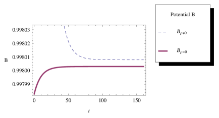
Figure 1: Temporal evolution of the gravitational potential $B$ at the stellar surface

3.2 Temporal evolution of the fluid pressure $p_{\Sigma}$

Here we examine the temporal behavior of the radiating fluid pressure at the boundary of the object. The pressure, for the two cases, is defined by the junction condition $(\ref{gjc})$. Fig. 2 shows that for the case of pressureless radiation only, the fluid pressure $p_{s}$, at the boundary is very small $(p\approx 4\times 10^{-4})$ and decreases monotonically with time until it is negligible. This is consistent with what has been theoretically established for stellar models in both the Newtonian and relativistic limits. On the other hand, in Figure 3 it can be seen that when $\rho\neq 0$, $p$ is slightly suppressed and becomes negative at the boundary. This is not surprising considering the general form of $(\ref{gjc})$. Another reason that supports this result is that when $\rho=0$, the pressure is already close to zero, and if the density which is always strictly positive (however small in magnitude it may be) is taken into account it is clear that this will induce a further reduction. We have also investigated the effect of varying the magnitude of $\rho$ and the family of profiles in Fig. 3 reveal that as the density is increased within the the allowed range, the pressure becomes increasingly more negative. This trend suggests that $p$ scales inversely with $\rho$ at the surface of the radiating star. It should be emphasized that despite this behaviour, the pressure is still only just slightly negative and does not in any way make the model physically unreasonable.

Figure 2: Temporal evolution of the radiating fluid pressure in the absence of $\rho$

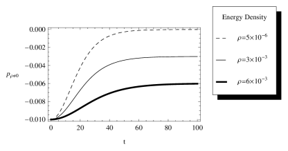
Figure 3: Temporal evolution of the radiating fluid pressure in the presence of $\rho$ with varying magnitudes

3.3 Temporal evolution of the fluid luminosity $L_{\Sigma}$

Utilising the definitions (19a) and (19b) along with the solution $(\ref{exactsolution})$ we are able to generate numerical profiles for the luminosity of the radiating fluid at the surface of the relativistic body and the luminosity as seen by a distant observer. In Fig. 4 we find that $L_{\Sigma}$ evolves in an acceptable manner and decreases through positive values until it eventually becomes substantially low. The plot also indicates that the initial magnitude of the luminosity at the boundary is very small $(L_{\Sigma}\approx 2.0\times 10^{-2})$, which may be justifiable for stellar objects that are ultra-dense and possibly in the post neutron star phase of its evolution. After an extended but finite period of time the star becomes virtually non-luminous and may not be observable. This is certainly consistent with the fact that the so called quark and quark-gluon stars have not yet been detected with current observing instruments. The family of profiles in Fig. 5 exhibits very interesting behaviour for $L_{\Sigma}$ in the more general situation when $\rho$ is non-vanishing. In general, the luminosity is suppressed and changes through negative values as the magnitude of $\rho$ is increased; $L_{\Sigma}$ at early times is less negative, and at late times tends to zero. The overall behaviour is similar to that found in Fig. 4 and again may be applicable to stars in the strong gravity regime. In Fig. 7, when there is only radiation in the exterior, the luminosity at infinity is singular closer to the centre of the fluid distribution and evolves through positive but small values with $r$. It is also clear that for large $r$ $(r\rightarrow\infty)$, $L_{\infty}$ tends to zero. This suggests that a horizon will form at the end of the collapse of the radiating object. Fig. 6 on the other hand indicates that $L_{\infty}$, when $\rho\neq 0$, is finite at $r=0$ and evolves through negative values until eventually going to zero. Again, this behaviour demonstrates the formation of a horizon at late times.

Figure 4: Temporal evolution of the radiating fluid luminosity in the absence of $\rho$

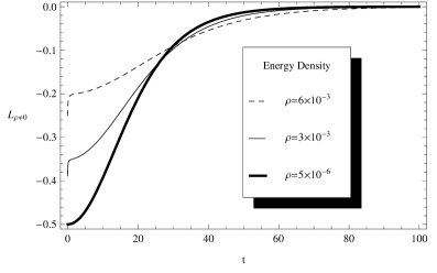
Figure 5: Temporal evolution of the radiating fluid luminosity in the presence of $\rho$ with varying magnitudes

Figure 6: Temporal profile of the radiating fluid luminosity at infinity in the presence of $\rho$

Figure 7: Temporal profile of the radiating fluid luminosity at infinity in the absence of $\rho$

3.4 Temporal evolution of the gravitational redshift $Z_{\Sigma}$

The plots in Fig. 8 show that $Z_{\rho\neq 0}>Z_{\rho=0}$ always. Furthermore, it is clear that the redshift, in both the standard Vaidya and generalised Vaidya models, evolves continuously and regularly through negative values. This is probably largely due to the nature of the exact solutions.

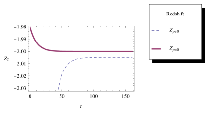
Figure 8: Temporal evolution of the gravitational redshift at the stellar surface

3.5 Mass flow across the boundary

Here we investigate the temporal behaviour of the mass flow and rate of mass flow at the radiating surface. The numerical profile in Fig. 9 illustrates that in the case of null dust $(\rho=0)$, the mass flow across the radiating surface decreases steadily with time, through positive values, until it terminates completely at later times. The situation when the flow of mass stops altogether corresponds to when the stellar object departs from its radiative phase and transits into an equilibrium state, usually towards the very late stages of gravitational collapse. For the model where the additional null fluid $(\rho\neq 0)$ is present in the exterior, Fig. 10 indicates that $m$ increases steadily with time and eventually converges to a non-zero limiting value. At this point the star is still losing mass but at a uniform rate. Hence, we may conclude that in the standard Vaidya model the mass flow naturally comes to a stop. However, in the more realistic and generalised Vaidya case, mass continues to flow across the boundary for an extended period of time. This is strong motivation for the idea that the null fluid distribution in the local exterior is actually sourced from within the radiating body and is released along with radiation during dissipation. This must then mean that the null fluid is more likely to be a distribution of particles like neutrinos which is consistent with what is believed to be the case for most compact objects (see the earlier treatments of Misner ⁴¹ and Glass ⁴⁰). In Fig. 11 we observe that mass flow rate across the surface, decreases fairly rapidly and ultimately goes to zero when the flow ceases. The profile in Fig. 12 indicates that for $\rho\neq 0$ $(dm/dt)$ is always negative and would seem to contradict the profile in Fig. 10. This is probably due to the form of the gravitational potential in the solution $(\ref{exactsolution})$ and the choice of parameter values that have been considered.

Figure 9: Temporal evolution of the mass flow across the stellar surface, in the absence of $\rho$

Figure 10: Temporal evolution of the mass flow across the stellar surface, in the presence of $\rho$

Figure 11: Temporal evolution of the mass flow rate across the stellar surface, in the absence of $\rho$

Figure 12: Temporal evolution of the mass flow rate across the stellar surface, in the presence of $\rho$

3.6 Energy conditions with $\rho\neq 0$

In any radiating relativistic model in astrophysics, a test of the strong, dominant and weak energy conditions are imperative in order to establish whether the model is valid and physically reasonable. This has been demonstrated in the seminal study by Kolassis et al ⁵⁰ and in the recent treatment by Govender et al ^gov12, for dense stellar objects with heat conduction. The weak, dominant, and strong energy conditions are described respectively, in the generalised Vaidya spacetime, by the following

$$W=\mu-\left(qB-\rho\right)+\Delta\geq 0,$$ (35a)

$$D=\mu-3\left(qB-\rho\right)+\Delta\geq 0,$$ (35b)

$$S=\left(qB-\rho\right)+\Delta\geq 0,$$ (35c)

where $\Delta$ is given by

$$\Delta=\sqrt{\left[\left(qB-\rho\right)+q\right]^{2}-4q^{2}}.$$ (36)

In the limit when $\rho=0$ the classical definitions for the energy conditions are regained.

The corresponding numerical profiles for the parameters $W$, $D$, and $S$ are given in Fig. 13-15. Fig. 13 demonstrates that the weak energy condition is satisfied since the parameter $W$ is regular, continuous and non-negative for all times. The dominant energy condition is also obeyed as seen from the profile for $D$ in Fig. 14. However, the strong energy condition is clearly violated since $S$ is always non-positive, in Fig. 15. We must point out, though, that this result is not entirely detrimental for the model since it has been established by Kolassis et al ⁵⁰, that the strong energy condition can be allowed to fail provided that the overall pressure of the matter distribution is negative. This works perfectly well with the generalised model with $m=m(v,r)$ since the pressure $P$ of the null fluid is negative for a constant density (as highlighted earlier in section 2.2) and in addition, the radiating fluid pressure is also negative (from Fig. 3), at the surface of the star. We may then conclude that the generalised null fluid model satisfies collectively, all of the energy conditions and remains physically acceptable.

Figure 13: Temporal evolution of the weak energy condition parameter at the radiating surface, subject to the influence of the null fluid energy density $\rho$

Figure 14: Temporal evolution of the dominant energy condition parameter at the radiating surface, subject to the influence of the null fluid energy density $\rho$

Figure 15: Temporal evolution of the strong energy condition parameter at the radiating surface, subject to the influence of the null fluid energy density $\rho$

3.7 The influence of the exterior null fluid on the nonadiabatic gravitational collapse of the relativistic star

A relativistic star can radiate away its heat energy in two possible scenarios: in the process of nonadiabatic gravitational collapse and when the object is in hydrostatic equilibrium undergoing thermal cooling. Our exact solution can be applied to the former case in particular and it would be a point of interest to determine what effect the exterior null fluid energy density $\rho$ could have on the collapse rate at the boundary.

The rate $\Theta$ of gravitational collapse for a spherically symmetrical shear-free fluid with geodesic particles is given by

$$\Theta = \frac{3\dot{B}}{AB},$$ (37)

for a comoving 4-velocity $u^{a}=\delta^{a}_{0}$. With the solution $(\ref{exactsolution})$, for the situation where the additional null fluid is present on the outside, the analytical form for the rate of collapse is

$$\Theta_{\rho\neq 0}=\frac{3\left(b^{2}-r^{2}\right)\left(b^{2}d^{2}\rho-\alpha^{2}\right)\operatorname{sech}\left[\frac{1}{2}t\sqrt{\frac{\alpha^{2}}{b^{2}d^{2}}-\rho}\right]^{2}}{2bd\left[\left(b^{2}+r^{2}\right)\alpha+bd\left(b^{2}-r^{2}\right)\sqrt{\frac{\alpha^{2}}{b^{2}d^{2}}-\rho}\tanh\left[\frac{1}{2}t\sqrt{\frac{\alpha^{2}}{b^{2}d^{2}}-\rho}\right]\right]}.$$ (38)

In the standard Vaidya model considered by Thirukkanesh and Maharaj ³⁸, with $\rho=0$, we have that

$$\Theta_{\rho=0}=\frac{3\alpha\left(b^{2}-r^{2}\right)\exp\left(\frac{\alpha(t+e)}{bd}\right)}{\left[r^{2}-\exp\left(\frac{\alpha(t+e)}{bd}\right)\right]\left[b^{2}-\exp\left(\frac{\alpha(t+e)}{bd}\right)\right]}.$$ (39)

It is quite clear from equations $(\ref{gencrate})$ and $(\ref{stdcrate})$ that in the general case $\Theta_{\rho\neq 0}$ has a strong dependence on the density $\rho$ and is far more involved than in the standard case $\Theta_{\rho=0}$. The numerical profiles corresponding to $(\ref{gencrate})$ and $(\ref{stdcrate})$ are given respectively by Fig. 16 and 17.

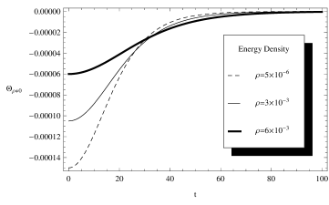
Figure 16: The collapse rate for varying null fluid energy density

Figure 17: The collapse rate for $\rho=0$

From Fig. 16 it is evident that the rate of collapse is negative when the null fluid is present in the exterior of the radiating body. In other words the non-vanishing energy density $\rho$ actually slows down the collapse process until such time when it reaches a complete halt and the relativistic star becomes stable again. It can also be seen that as the magnitude of the density is increased, $\Theta_{\rho\neq 0}$ becomes less negative at earlier times and eventually goes to zero at late times. The plot in Fig. 17 illustrates that for vanishing density, the rate of collapse is always positive and indicates that the collapse itself is occurring reasonably faster.

4 Discussion

In this paper we modeled a spherically symmetric relativistic radiating star that has vanishing shearing stresses and radial heat flow in the interior while its local exterior region consists of a two-fluid system comprising pressureless radiation and a general null fluid. The Type II fluid possesses a non-zero pressure and energy density and in particular we have investigated the influence of the density $\rho$ on the physical behaviour of the dissipating stellar fluid at the surface. We demonstrated that the generalised junction condition $p=qB-\rho$ for a null fluid scenario can be integrated as a nonlinear differential equation, at the boundary and generated an exact solution in the special case when the interior fluid particles are in geodesic motion and the exterior density is constant. Our solution, although similar in structure to that obtained by Govender and Thirukkanesh ⁴³, has a very different interpretation, depending strongly on the magnitude of $\rho$ and can be cast in a more realistic astrophysical context. The generalised two-fluid model with our exact solution has been compared to the standard model for pure radiation, studied by Thirukkanesh and Maharaj ³⁸, by constructing numerical profiles for various physical parameters associated with the stellar fluid at the boundary.

We established that the constant null fluid energy density has a marked impact and significantly reduces the pressure $p_{\Sigma}$ and luminosity $L_{\Sigma}$ when compared to the limiting case when $\rho=0$, where the pressure and luminosity are positive, finite and consistent with well established results for extremely dense stellar objects in the strong gravity regime. The flow of mass across the radiating surface was also probed and it has been demonstrated that the density $\rho$ actually enhances the outgoing flow; this is suggestive that the null fluid on the outside could more likely be interpreted as a distribution of particles that are sourced from nonadiabatic and particle production processes originating within and at the surface of the star. This is in contrast to other treatments where the null fluid has been considered to be an ambient string system in four dimensions. In light of this our model may offer a more realistic description for dense stars in a relativistic setting. By utilising the interior matter variables and the exact solution $(\ref{exactsolution})$ we also tested the strong, dominant and weak energy conditions when the constant density null fluid is prevalent. Numerical profiles indicate that the weak and dominant conditions are satisfied while the strong condition is violated. However this does not severely affect the validity of the model in any way as the overall pressure is negative. Since radiating models are crucial for studying the nonadiabatic gravitational collapse of stellar objects, the rate of collapse, for both situations has also been examined. It has been found that $\rho$ slows down the collapse process while in the case of null radiation only it occurs faster. Our model can be further improved on by including the effects of shear and bulk viscosity and analysing the dynamical stability of the stellar matter configuration. Furthermore, if the null fluid is to be taken as a system of particles like neutrinos for example then the model can be appropriately adapted by incorporating non-vanishing neutrino fluxes in the interior. However, these considerations would consequently render the model more complicated and in particular the junction condition increasingly difficult to solve, even with the robust mathematical techniques that are currently available. These endeavors will be the subject of an ongoing investigation.

Acknowledgements

GG, BPB and SDM thank the National Research Foundation and the University of KwaZulu-Natal for financial support. SDM acknowledges that this work is based upon research supported by the South African Research Chair Initiative of the Department of Science and Technology and the National Research Foundation. We thank Søren Greenwood for his assistance with computing software related issues. The authors would also like to thank Dr. Megandhren Govender and Dr. Rituparno Goswami for constructive criticisms and useful discussions.

References

- 1 Oppenheimer J R and Snyder H, On continued Gravitational Contraction, Phys. Rev. 56, 455-459 (1939).
- 2 Penrose R, Gravitational collapse: The role of general relativity, Rivista del Nuovo Cimento 1, 257 (1969).
- 3 Glendenning N K, Compact Stars: Nuclear Physics, Particle Physics, and General Relativity, (Springer, New York) (2000).
- 4 Strauman N, General Relativity With Applications to Astrophysics, (Springer, Berlin) (2004).
- 5 Shapiro S L and Teukolsky S A, Black Holes, White Dwarfs, and Neutron Stars: The Physics of Compact Objects, (Wiley-VCH, New York) (1983).
- 6 Vaidya P C, The gravitational field of a radiating star, Proc. Indian Acad. Sc. A 33, 264 (1951).
- 7 Santos N O, Nonadiabatic radiating collpse, Mon. Not. R. Astron. Soc. 216, 403-410 (1985).
- 8 Maharaj S D, Govender G and Govender M, Radiating stars with generalised Vaidya atmospheres, Gen. Relativ. Gravit. 44, 1089-1099 (2012).
- 9 de Olioveira A K G and Santos N O, Nonadiabatic gravitational collapse, Astrophys. J. 312, 640-645 (1987).
- 10 Maharaj S D and Govender G, Collapse of a charged radiating star with shear, Pramana 54, 715-727 (2000).
- 11 Pinheiro G and Chan R, Radiating shear-free gravitational collapse with charge, Gen. Relativ. Gravit. 45, 243-261 (2013).
- 12 Chan R, Collapse of a radiating star with shear, Mon. Not. R. Astron. Soc. 288, 589-595 (1997).
- 13 Chan R, Radiating gravitational collpase with shearing motion and bulk viscosity, Astronomy and Astrophysics 368, 325-334 (2001).
- 14 Pinheiro G and Chan R, Radiating gravitational collapse with shear viscosity revisited, Gen. Relativ. Gravit. 40, 2149-2175 (2008).
- 15 Misthry S S, Maharaj S D and Leach P G L, Nonlinear shear-free radiative collapse, Math. Meth. Appl. Sci. 31, 363 (2008).
- 16 Abebe G Z, Govinder K S and Maharaj S D, Lie symmetries for a conformally flat radiating star, Int. J. Theor. Phys. 52, 3244-3254 (2013).
- 17 Abebe G Z, Maharaj S D and Govinder K S, Geodesic models generated by Lie symmetries, Gen. Relativ. Gravit. 46, 1650 (2014).
- 18 Abebe G Z, Maharaj S D and Govinder K S, Generalised Euclidean stars with equation of state, Gen. Relativ. Gravit. 46, 1733 (2014).
- 19 Maharaj S D and Govender M, Radiating collpase with vanishing Weyl stresses, Int. J. Mod. Phys. D 14, 667 (2005).
- 20 Martinez J, Transport processes in the gravitational collapse of an anisotropic fluid, Phys. Rev. D 53, 6921-6940 (1996).
- 21 Herrera L and Santos N O, Thermal evolution of compact objects and relaxation time, Mon. Not. R. Astron. Soc. 287, 161-164 (1997).
- 22 Govender M, Maartens R and Maharaj S D, Relaxational effects in radiating stellar collapse, Mon. Not. R. Astron. Soc. 310, 557-564 (1999).
- 23 Naidu N F, Govender M and Govinder K S, Thermal evolution of a radiating anisotropic star with shear, Int. J. Mod. Phys. D 15, 1053 (2006).
- 24 Naidu N F and Govender M, Causal temperature profiles in horizon-free collapse, J. Astrophys. Astron. 28, 167-174 (2008).
- 25 Maharaj S D, Govender G and Govender M, Temperature evolution during dissipative collapse, Pramana J. Phys. 77, 469-476 (2011).
- 26 Wagh S M, Govender M, Govinder K S, Maharaj S D, Muktibodh P S and Moodley M, Shear-free spherically symmetric spacetimes with an equation of state , Class. Quant. Grav. 18, 2147 (2001).
- 27 Goswami R and Joshi P S, Gravitational collapse of an isentropic perfect fluid with a linear equation of state, Class. Quant. Grav. 21, 3645-3654 (2004).
- 28 Sharma R and Maharaj S D, A class of relativistic stars with a linear equation of state, Mon. Not. R. Astron. Soc. 375, 1265 (2007).
- 29 Husain V, Exact solutions for null fluid collapse, Phys. Rev. D 53, 1759-1762 (1996).
- 30 Wang A and Wu Y, Generalized Vaidya solutions, Gen. Relativ. Gravit. 31, 107-114 (1999).
- 31 Krisch J P and Glass E N, Energy transport in the Vaidya system, J. Math Phys. 46, 062501 (2005).
- 32 Yang I C, On the energy of the Vaidya spacetime, Chin. J. Phys. 45, 497-503 (2007).
- 33 Glass E N and Krisch J P, Radiation and string atmosphere for relativistic stars, Phys. Rev. D 57, R5945-R5947 (1998).
- 34 Glass E N and Krisch J P, Two-fluid atmosphere for relativistic stars, Class. Quantum Grav. 16, 1175-1184 (1999).
- 35 Vilenkin A, Cosmic strings, Phys. Rev. D 24, 2082-2089 (1981).
- 36 Percival I C, Quantum spacetime fluctuations and primary state diffusion, Proc. R. Soc. A 451, 503-513 (1995).
- 37 Percival I C and Strunz W T, Detection of spacetime fluctuations by a small interferometer, Proc. R. Soc. A 453, 431-446 (1997).
- 38 Thirukkanesh S and Maharaj S D, Radiating relativistic matter in geodesic motion, J. Math. Phys. 50, 022502 (2009).
- 39 Hawking S W and Ellis G F R, The large scale structure of spacetime (Cambridge: Cambridge University Press) (1973).
- 40 Glass E N, A spherical collapse solution with neutrino outflow, J. Math. Phys. 31, 1974-1977 (1990).
- 41 Misner C W, Relativistic equations for spherical gravitational collpase with escaping neutrinos, Phys. Rev. 137, 1360 (1965).
- 42 Rajah S S and Maharaj S D, A Riccati equation in radiative stellar collapse, J. Math. Phys. 49, 012501 (2008).
- 43 Govender M and Thirukkanesh S, Dissipative collapse in the presence of , Int. J. Theor. Phys. 48, 3558-3566 (2009).
- 44 Banerjee A, Dutta Choudhury S B and Bhui B K, Conformally Flat Solutions with Heat Flux, Phys. Rev. 40, 670 (1989).
- 45 Kolassis C A, Santos N O and Tsoubelis D, Friedmann-like collapsing model of a radiating sphere with heat flow, Astrophys. J. 327, 755-759 (1988).
- 46 Bonnor W B, de Oliveira A K G and Santos N O, Radiating spherical collapse, Physics Reports 181, 269-326 (1989).
- 47 Tewari B C, Relativistic model for a radiating star, Astrophys Space Sci 306, 273-277 (2006).
- 48 Sarwe S and Tikekar R, Nonadiabatic gravitational collapse of a superdense star, Int. J. Mod. Phys. D 19, 1889-1904 (2010).
- 49 Hladik J and Stuchlik Z, Photon and neutrino redshift in the field of braneworld compact stars, arXiv: 1108.5760v1 gr-qc (2011).
- 50 Kolassis A C, Santos N O and Tsoubelis D, Energy conditions for an imperfect fluid, Class. Quantum Grav. 5, 1329-1339 (1988).