Finite Volume Evolution Galerkin Methods for the Shallow Water Equations with Dry Beds

Abstract

We present a new Finite Volume Evolution Galerkin (FVEG) scheme for the solution of the shallow water equations (SWE) with the bottom topography as a source term. Our new scheme will be based on the FVEG methods presented in (Lukáčová, Noelle and Kraft, J. Comp. Phys. 221, 2007), but adds the possibility to handle dry boundaries. The most important aspect is to preserve the positivity of the water height. We present a general approach to ensure this for arbitrary finite volume schemes. The main idea is to limit the outgoing fluxes of a cell whenever they would create negative water height. Physically, this corresponds to the absence of fluxes in the presence of vacuum. Well-balancing is then re-established by splitting gravitational and gravity driven parts of the flux. Moreover, a new entropy fix is introduced that improves the reproduction of sonic rarefaction waves.

65M08, 76B15, 76M12, 35L50 02.60.Cb, 47.11.Df, 92.10.Sx

1 Introduction

The shallow water equations (SWE) are a mathematical model for the movement of water under the action of gravity. Mathematically spoken, they form a set of hyperbolic conservation laws, which can be extended by source terms like the influence of the bottom topography, friction or wind forces. In this case, we will speak of a balance law. For simplicity, this work will consider the variation of the bottom as the only source term.

Many important properties of the model rely on the fact that the water height is strictly positive. Despite this, typical relevant problems include the occurrence of dry areas, like dam break problems or the run-up of waves at a coast, with tsunamis as the most impressive example. So for simulations of these problems, we have to develop numerical schemes that can handle the (possibly moving) shoreline in a stable and efficient way. Another crucial point in solving balance laws is the treatment of the source terms. For precise solutions, it is necessary to evaluate the source term in such a way that certain steady states are kept numerically, i.e. the numerical flux and the numerical source term cancel each other exactly for equilibrium solutions.

In the last years, many groups contributed to the solution of the difficulties described above. In [AudusseBouchutBristeauEtAl2004], Audusse et al. proposed a reconstruction procedure where the free surface and water height are reconstructed and the bottom slopes are computed from these. This guarantees the positivity of the water height and gives a well-balanced scheme at the same time. Begnudelli and Sanders developed a scheme for triangular meshes including scalar transports in [BegnudelliSanders2006]. They proposed a strategy how to exactly represent the free surface in partially wetted cells, leading to improved results at the wetting/drying front. In [BrufauVazquez-CendonGarcia-Navarro2002], Brufau et al. analyse how to deal with flow on an adverse slope. They locally modify the bottom topography in certain situations to avoid unphysical run-ups or wave creation at the dry boundary. Gallardo et al. discussed various solutions of the Riemann problem at the front and used them in a modified Roe scheme. They then used the local hyperbolic harmonic method from Marquina (cf. [Marquina1994]) in the reconstruction step to achieve higher order, see [GallardoParesCastro2007]. Kurganov and Petrova proposed a central-upwind scheme that is well-balanced and positivity preserving in [KurganovPetrova2007]. It is based on a continuous, piecewise linear approximation of the bottom topography and performs the computation in terms of the free surface instead of the relative water height to simplify the well-balancing. The last feature is also a building block in the work of Liang and Marche [LiangMarche2009]. They also provide a method to extend this well-balancing feature to situations including wetting/drying fronts. Liang and Borthwick [LiangBorthwick2009] used adaptive quad-tree grids to improve the efficiency of their schemes. Wetting and drying effects are handled as well as friction terms. In the context of residual distribution methods, Ricchiuto and Bollermann developed a positivity preserving and well-balanced scheme for unstructured triangulations [RicchiutoBollermann2009].

The finite volume evolution Galerkin (FVEG) methods developed by Lukáčová, Morton and Warnecke, cf. [LukacovaMortonWarnecke2004, LukacovaSaibertovaWarnecke2002, LukacovaNoelleKraft2007], have been successfully applied to the SWE in [LukacovaNoelleKraft2007]. They are based on the evaluation of so called evolution operators which predict values for the finite volume update. Thanks to these operators, the schemes take into account all directions of wave propagation, enabling them to precisely catch multidimensional effects even on Cartesian grids. These schemes show a very good accuracy even on relatively coarse meshes compared to other state of the art schemes and they are also competitive in terms of efficiency (cf. [LukacovaNoelleKraft2007]).

However, the existing FVEG schemes are not able to deal with dry boundaries. Thus in this work we will present a method to preserve the positivity of the water height with an arbitrary finite volume method. To achieve this, we reduce the outflow on draining cells such that the water height does not become negative. We will then provide the means to preserve the well-balancing property under the presence of dry areas, and apply both techniques to a new FVEG method. In addition, we present a new entropy fix for the FVEG schemes that improves the reproduction of sonic rarefaction waves.

We start our paper with a short presentation of the SWE in Section 2. Section 3 describes the FVEG method we will start from. The arising difficulties by introducing dry areas and means to overcome them are described in Section 4, which is the main part of the paper. Finally, in Section 5, we will show selected numerical test cases that demonstrate the performance of our schemes.

2 The Shallow Water Equations

2.1 Balance Law Form

We consider the shallow water system in balance form

$$\frac{\partial{\mathbf{u}}}{\partial t}+\nabla\cdot\boldsymbol{\mathcal{F}}({\mathbf{u}})=-\boldsymbol{\mathcal{S}}({\mathbf{u}},\vec{x}).$$ (1)

The conserved variables and the flux are given by

$${\mathbf{u}}=\begin{pmatrix}h\\ hv_{1}\\ hv_{2}\end{pmatrix},\quad\boldsymbol{\mathcal{F}}({\mathbf{u}})=\left(\boldsymbol{\mathcal{F}}_{1}({\mathbf{u}})\,\boldsymbol{\mathcal{F}}_{2}({\mathbf{u}})\right)=\begin{pmatrix}hv_{1}&hv_{2}\\ hv_{1}^{2}+g\frac{h^{2}}{2}&hv_{1}v_{2}\\ hv_{1}v_{2}&hv_{2}^{2}+g\frac{h^{2}}{2}\end{pmatrix},$$ (2)

where $h$ denotes the relative water height, ${\vec{v}}=(v_{1},v_{2})^{T}$ the flow speed and $g$ the (constant) gravity acceleration. The source term $\boldsymbol{\mathcal{S}}({\mathbf{u}},\vec{x})$ is given by

$$\boldsymbol{\mathcal{S}}({\mathbf{u}},\vec{x})=gh\begin{pmatrix}0\\ \frac{\partial b(\vec{x})}{\partial x_{1}}\\ \frac{\partial b(\vec{x})}{\partial x_{2}}\end{pmatrix}$$ (3)

with $b(\vec{x})$ the local bottom height. We also introduce the free surface level, or total water height,

$$H(\vec{x})=h(\vec{x})+b(\vec{x})$$ (4)

and the so-called speed of sound

$$c=\sqrt{gh}.$$ (5)

This is the velocity of the gravity waves and should not be confused with the physical sound speed in air.

2.2 Quasi-linear Form

For the derivation of the evolution operators in Section 3.2, it is helpful to rewrite (1) in primitive variables. The system then takes the form

$${\mathbf{w}}_{t}+{\mathbf{A}}_{1}({\mathbf{w}}){\mathbf{w}}_{x_{1}}+{\mathbf{A}}_{2}({\mathbf{w}}){\mathbf{w}}_{x_{2}}={\mathbf{t}}$$ (6)

with

$${\mathbf{w}}=\begin{pmatrix}h\\ v_{1}\\ v_{2}\end{pmatrix},\quad{\mathbf{A}}_{1}=\begin{pmatrix}v_{1}&h&0\\ g&v_{1}&0\\ 0&0&v_{1}\end{pmatrix},\quad{\mathbf{A}}_{2}=\begin{pmatrix}v_{2}&0&h\\ 0&v_{2}&0\\ g&0&v_{2}\end{pmatrix}$$ (7)

and the source term

$${\mathbf{t}}=\begin{pmatrix}0\\ -gb_{x_{1}}\\ -gb_{x_{2}}\end{pmatrix}.$$ (8)

For each angle $\theta\in[0,2\pi)$ we define the direction $\vec{\xi}(\theta):=(\cos\theta,\sin\theta)$. As system (1) is hyperbolic, for each of these directions and a fixed ${\mathbf{w}}$ the matrix

$${\mathbf{A}}({\mathbf{w}})=\vec{\xi}_{1}{\mathbf{A}}_{1}({\mathbf{w}})+\vec{\xi}_{2}{\mathbf{A}}_{2}({\mathbf{w}})$$ (9)

has real eigenvalues

$$\lambda_{1}={\vec{v}}\cdot\vec{\xi}-c,\quad\lambda_{2}={\vec{v}}\cdot\vec{\xi},\quad\lambda_{3}={\vec{v}}\cdot\vec{\xi}+c$$ (10)

and a full set of linearly independent eigenvectors

$$r_{1}=\begin{pmatrix}-1\\ g\frac{\cos\theta}{c}\\ g\frac{\sin\theta}{c}\end{pmatrix},\quad r_{2}=\begin{pmatrix}0\\ \sin\theta\\ -\cos\theta\end{pmatrix},\quad r_{3}=\begin{pmatrix}1\\ g\frac{\cos\theta}{c}\\ g\frac{\sin\theta}{c}\end{pmatrix}.$$ (11)

2.3 Lake at Rest

A trivial, but nevertheless important solution to (1) is the lake at rest situation, where the water is steady and the free surface level is constant, i.e. we have

$${\vec{v}}=(0,0)^{T}\text{ and }H(\vec{x})=H_{0}.$$ (12)

From (4) we immediately get

$$\nabla h=-\nabla b$$ (13)

and therefore (with (1) – (3) and ${\vec{v}}=(0,0)^{T}$)

$$\begin{pmatrix}0\\ g\frac{h^{2}}{2}\\ 0\end{pmatrix}_{x_{1}}+\begin{pmatrix}0\\ 0\\ g\frac{h^{2}}{2}\end{pmatrix}_{x_{2}}=-gh\begin{pmatrix}0\\ \frac{\partial b(\vec{x})}{\partial x_{1}}\\ \frac{\partial b(\vec{x})}{\partial x_{2}}\end{pmatrix}.$$ (14)

A scheme fulfilling a discrete analogon of (14) exactly is called well-balanced.

3 FVEG Schemes

Finite volume schemes are very popular for solving hyperbolic conservation laws for several reasons. They represent the underlying physics in a natural way and can be implemented very efficiently. Nevertheless, nearly all of them are based on the solution of one-dimensional Riemann problems and therewith a dimensional splitting. This introduces some sort of a bias: Wave propagation aligned with the grid is very well represented, whereas waves oblique to the grid cannot be caught as accurate.

In the last decade Lukáčová et al. developed a class of finite volume evolution Galerkin schemes, see e.g. [LukacovaMortonWarnecke2000, LukacovaSaibertovaWarnecke2002, LukacovaWarneckeZahaykah2004]. The FVEG scheme is a predictor-corrector method: In the predictor step a multidimensional evolution is done, the corrector step is a finite volume update.

In this section we will recall the second order scheme presented in [LukacovaNoelleKraft2007]. This method will be the starting point for our extensions for computations including dry beds in Section 4. Therefore we concentrate on the properties playing a role in this context and limit ourselves to the main ideas otherwise.

3.1 Finite Volume Update

For our computations, we use Cartesian grids, i.e. we divide our computational domain $\Omega$ in rectangular cells $C_{i}$, separated by edges $E$. On the edges, we have quadrature points ${\vec{x}}_{k}$. The subscript $i$ will always refer to a cell, whereas $k$ as a subscript is used as a global index for quadrature points. If we talk about the local quadrature points on a single edge, we use the index $j$ instead.

On each cell we define the initial value at as

$${\mathbf{u}}_{i}^{0}:={\mathbf{u}}_{i}(0)\approx\frac{1}{|C_{i}|}\int_{C_{i}}{\mathbf{u}}(\vec{x},0)\,d\vec{x}$$ (15)

where we use a Gaussian quadrature to approximate the integral. Integrating (1) on each cell, we can then define the update as

$${\mathbf{u}}_{i}^{n+1}={\mathbf{u}}_{i}^{n}-\frac{1}{|C_{i}|}\int_{t^{n}}^{t^{n+1}}\left(\int_{\partial C_{i}}\boldsymbol{\mathcal{F}}({\mathbf{u}}(\vec{x},t))\cdot\vec{n}\,d\vec{x}+\int_{C_{i}}\boldsymbol{\mathcal{S}}({\mathbf{u}}({\vec{x}},t),{\vec{x}})\,d\vec{x}\right)dt$$ (16)

using the Gauss theorem. Here ${\mathbf{u}}_{i}^{n}$ denotes cell average in $C_{i}$ at time $t^{n}$ and $\vec{n}$ is the outer normal. The solution on the whole domain at time $t^{n}$ is then defined as

$${\mathbf{U}}^{n}({\vec{x}}):={\mathbf{U}}({\vec{x}},t^{n})={\mathbf{u}}_{i}^{n},\quad{\vec{x}}\in C_{i}.$$ (17)

For an approximation of (16), on each edge we define three quadrature points $\vec{x}_{j},j=1,2,3$, see Fig. 1.

Figure 1: Quadrature points $\vec{x}_{j}$ for finite volume update

These quadrature points are located on the vertices ($j=1,3$) and the centre ($j=2$) of an edge. The flux over the edge is approximated by using midpoint rule in time and Simpson’s rule in space, hence we will use the evolution operators from Section 3.2 to predict point values at the quadrature points at time $t^{n+1/2}$. The flux over an edge is then defined as

$$\boldsymbol{\mathcal{F}}_{E}:=\sum_{j=1}^{3}\alpha_{j}\boldsymbol{\mathcal{F}}({\mathbf{u}}_{j}^{n+1/2})\cdot\vec{n}\approx\frac{1}{\Delta t|E|}\int_{t^{n}}^{t^{n+1}}\int_{E}\boldsymbol{\mathcal{F}}({\mathbf{u}}(\vec{x},t))\cdot\vec{n}\,d\vec{x}dt.$$ (18)

$\Delta t=t^{n+1}-t^{n}$ is the time step, ${\mathbf{u}}_{j}^{n+1/2}$ is an approximation to ${\mathbf{u}}({\vec{x}}_{j},t^{n+1/2})$ and the $\alpha_{j}$ represent the weights of Simpson’s rule, i.e. we have $\alpha_{1,3}=\frac{1}{6}$ and $\alpha_{2}=\frac{2}{3}$. Finally the source term is discretised as

$$\boldsymbol{\mathcal{S}}_{i}:=g\sum_{j=1}^{3}\alpha_{j}\begin{pmatrix}0\\ \frac{1}{2}(\hat{h}_{j}^{r}+\hat{h}_{j}^{l})(b_{j}^{r}-b_{j}^{l})\\ \frac{1}{2}(\hat{h}_{j}^{t}+\hat{h}_{j}^{b})(b_{j}^{t}-b_{j}^{b})\end{pmatrix}\approx\frac{1}{\Delta x\Delta t}\int_{t^{n}}^{t^{n+1}}\int_{C_{i}}\boldsymbol{\mathcal{S}}({\mathbf{u}})\,d\vec{x}.$$ (19)

Here, $\Delta x$ is the length of the element, $\hat{h}_{j}$ represents the first component of ${\mathbf{u}}_{j}^{n+1/2}$ and $b_{j}=b(\vec{x}_{j})$. The superscripts stand for the edges surrounding the cell, namely the right, left, top and bottom edge. Eqs. (16)–(19) lead to the fully discrete scheme

$${\mathbf{u}}_{i}^{n+1}={\mathbf{u}}_{i}^{n}-\frac{\Delta t}{\Delta x}\left[\left(\sum_{E,E\subset\partial C_{i}}\boldsymbol{\mathcal{F}}_{E}\right)+\boldsymbol{\mathcal{S}}_{i}\right].$$ (20)

The time step is chosen as

$$\Delta t=\mu\min_{i}\dfrac{\Delta x}{\max_{k}|\lambda_{k}|}$$ (21)

with $\lambda_{k}$ the eigenvalues from (10) and $\mu<1$ a CFL number. For all the numerical experiments in Section 5, we set $\mu=0.5$.

3.2 Evolution Operators

As mentioned before, we use so-called evolution operators to predict point values of the solution for the quadrature points in (18). Indeed, a solution of (6) can be seen as a superposition of waves. So for a fixed point $P=({\vec{x}},t)$, we want to identify all the waves that contribute to the solution there. This section will describe shortly the evolution operator, present an exact formulation and give an example of a suitable approximation allowing an efficient implementation.

The derivation of evolution operators is based on the quasi-linear form of the system (6). For any given point $P$, we identify a suitable average value $\bar{\mathbf{w}}$ and linearise the system around $P$:

$${\mathbf{w}}_{t}+{\mathbf{A}}_{1}(\bar{\mathbf{w}}){\mathbf{w}}_{x_{1}}+{\mathbf{A}}_{2}(\bar{\mathbf{w}}){\mathbf{w}}_{x_{2}}={\mathbf{t}}.$$ (22)

The waves we are looking for propagate along the characteristics of this system. Thus for a fixed direction $\vec{\xi}(\theta)$, we apply an one-dimensional characteristic decomposition of the linearised system. This allows us to identify different wave propagations corresponding to the eigenvalues (10), the bicharacteristics. The left side of Fig. 2 shows an illustration.

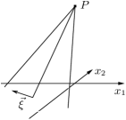
Figure 2: Bicharacteristic decomposition. Left: Bicharacteristic curves for a fixed direction $\vec{\xi}$. Right: Bicharacteristic cone.

Integrating the decomposed system along the bicharacteristics, we get an integral representation of the solution at point $P$. At this point, the solution still depends on a particular direction $\vec{\xi}(\theta)$ and therefore does not respect waves coming from other directions. Thus we perform the decomposition for all angles $\theta\in[0,2\pi)$ and average the solution at $P$ over $\theta$. This yields the exact evolution operator of (22). The combination of all bicharacteristics yields the bicharacteristic cone shown in the right picture of Fig. 2. We introduce the following notation for the peak $P=({\vec{x}},t^{n}+\tau)$ and points on the sonic cone:

$$Q_{0} :=(x_{1}+\tau\bar{v}_{1},\;x_{2}+\tau\bar{v}_{2},\;t^{n})$$ (23)

$${\tilde{Q}}_{0} :=(x_{1}+(t^{n}+\tau-\tilde{t})\bar{v}_{1}\cos\theta,\;x_{2}+(t^{n}+\tau-\tilde{t})\bar{v}_{2}\sin\theta,\;\tilde{t})$$ (24)

$$Q :=(x_{1}+\tau(\bar{c}+\bar{v}_{1})\cos\theta,\;x_{2}+\tau(\bar{c}+\bar{v}_{2})\sin\theta,\;t^{n})$$ (25)

$${\tilde{Q}} :=(x_{1}+(t^{n}+\tau-\tilde{t})(\bar{c}+\bar{v}_{1})\cos\theta,\;x_{2}+(t^{n}+\tau-\tilde{t})(\bar{c}+\bar{v}_{2})\sin\theta,\;\tilde{t})$$ (26)

$Q_{o}$ is the centre of the sonic circle at time $t=t^{n}$, ${\tilde{Q}}_{0}$ denotes a point on the inner bicharacteristic connecting $P$ and $Q_{0}$, $Q$ is a point on the perimeter of the sonic circle at time $t=t^{n}$ and ${\tilde{Q}}$ denotes a point on the mantle of the sonic cone at an arbitrary time $\tilde{t}\in[t^{n},t^{n}+\tau]$.

After some tedious calculations, see e.g. [LukacovaNoelleKraft2007], we get the evolution operators for the SWE:

$$\begin{split}h(P)&=\frac{1}{2\pi}\int_{0}^{2\pi}h(Q)-\frac{\bar{c}}{g}(v_{1}(Q)\cos\theta+v_{2}(Q)\sin\theta)\;d\theta\\ &\quad+\frac{\bar{c}}{2\pi}\int_{t}^{t+\tau}\int_{0}^{2\pi}(b_{x_{1}}({\tilde{Q}})\cos\theta+b_{x_{2}}({\tilde{Q}})\sin\theta)\;d\theta d\tilde{t}\\ &\quad-\frac{1}{2\pi}\int_{t}^{t+\tau}\frac{1}{t+\tau-\tilde{t}}\int_{0}^{2\pi}\frac{\bar{c}}{g}(v_{1}({\tilde{Q}})\cos\theta+v_{2}({\tilde{Q}})\sin\theta)\;d\theta d\tilde{t}\end{split}$$ (27)

$$\begin{split}v_{1}(P)&=\frac{1}{2}v_{1}(Q_{0})+\frac{1}{2\pi}\int_{0}^{2\pi}-\frac{g}{\bar{c}}h(Q)\cos\theta+v_{1}(Q)\cos^{2}\theta+v_{2}(Q)\sin\theta\cos\theta\;d\theta\\ &\quad-\frac{g}{2}\int_{t}^{t+\tau}h_{x_{1}}({\tilde{Q}}_{0})+b_{x_{1}}({\tilde{Q}}_{0})\;d\tilde{t}\\ &\quad-\frac{g}{2\pi}\int_{t}^{t+\tau}\int_{0}^{2\pi}(b_{x_{1}}({\tilde{Q}})\cos^{2}\theta+b_{x_{2}}({\tilde{Q}})\sin\theta\cos\theta)\;d\theta d\tilde{t}\\ &\quad+\frac{1}{2\pi}\int_{t}^{t+\tau}\frac{1}{t+\tau-\tilde{t}}\int_{0}^{2\pi}(v_{1}({\tilde{Q}})\cos 2\theta+v_{2}({\tilde{Q}})\sin 2\theta)\;d\theta d\tilde{t}\end{split}$$ (28)

$$\begin{split}v_{2}(P)&=\frac{1}{2}v_{2}(Q_{0})+\frac{1}{2\pi}\int_{0}^{2\pi}-\frac{g}{\bar{c}}h(Q)\sin\theta+v_{1}(Q)\sin\theta\cos\theta+v_{2}(Q)\sin^{2}\theta\;d\theta\\ &\quad-\frac{g}{2}\int_{t}^{t+\tau}h_{x_{2}}({\tilde{Q}}_{0})+b_{x_{2}}({\tilde{Q}}_{0})\;d\tilde{t}\\ &\quad-\frac{g}{2\pi}\int_{t}^{t+\tau}\int_{0}^{2\pi}(b_{x_{1}}({\tilde{Q}})\cos\theta\sin\theta+b_{x_{2}}({\tilde{Q}})\sin^{2}\theta)\;d\theta d\tilde{t}\\ &\quad+\frac{1}{2\pi}\int_{t}^{t+\tau}\frac{1}{t+\tau-\tilde{t}}\int_{0}^{2\pi}(v_{1}({\tilde{Q}})\sin 2\theta+v_{2}({\tilde{Q}})\cos 2\theta)\;d\theta d\tilde{t}.\end{split}$$ (29)

For efficient computations these operators have to be simplified. In [LukacovaNoelleKraft2007], the authors follow [LukacovaMortonWarnecke2004] and present approximations of (27) – (29) that provide exact solutions of some one-dimensional Riemann problems. For piecewise constant data, these approximations read

$$\begin{split}h(P)&=\frac{1}{2\pi}\int_{0}^{2\pi}\left[H(Q)-\frac{\bar{c}}{g}\left(v_{1}(Q)\operatorname{sgn}(\cos\theta)+v_{2}(Q)\operatorname{sgn}(\sin\theta)\right)\right]\;d\theta\\ &\quad-b(P)+\frac{\tau}{2\pi}\int_{0}^{2\pi}(\bar{v}_{1}b_{x_{1}}(Q)+\bar{v}_{2}b_{x_{2}}(Q))\;d\theta,\end{split}$$ (30)

$$\begin{split}v_{1}(P)&=\frac{1}{2\pi}\int_{0}^{2\pi}\left[-\frac{g}{\bar{c}}H(Q)\operatorname{sgn}(\cos\theta)\right.\\ &\quad\phantom{\frac{1}{2\pi}\int_{0}^{2\pi}}\quad\left.+v_{1}(Q)\left(\cos^{2}\theta+\frac{1}{2}\right)+v_{2}(Q)\sin\theta\cos\theta\right]\;d\theta,\end{split}$$ (31)

$$\begin{split}v_{2}(P)&=\frac{1}{2\pi}\int_{0}^{2\pi}\left[-\frac{g}{\bar{c}}H(Q)\operatorname{sgn}(\sin\theta)\right.\\ &\quad\phantom{\frac{1}{2\pi}\int_{0}^{2\pi}}\quad\left.+v_{1}(Q)\sin\theta\cos\theta+v_{2}(Q)\left(\sin^{2}\theta+\frac{1}{2}\right)\right]\;d\theta.\end{split}$$ (32)

The corresponding operators for piecewise (bi-)linear data are given as

$$\begin{split}h(P)&=H(Q_{0})(1-\frac{\pi}{2})-b(P)+\frac{1}{4}\int_{0}^{2\pi}H(Q)\;d\theta\\ &\quad-\frac{\bar{c}}{g\pi}\int_{0}^{2\pi}(v_{1}(Q)\cos\theta+v_{2}(Q)\sin\theta)\;d\theta\\ &\quad+\frac{\tau}{2\pi}\int_{0}^{2\pi}(\bar{v}_{1}b_{x_{1}}(Q)+\bar{v}_{2}b_{x_{2}}(Q))\;d\theta,\end{split}$$ (33)

$$\begin{split}v_{1}(P)&=v_{1}(Q_{0})(1-\frac{\pi}{4})+\frac{g}{\bar{c}\pi}\int_{0}^{2\pi}H(Q)\cos\theta\;d\theta\\ &\quad+\frac{1}{4}\int_{0}^{2\pi}\left[v_{1}(Q)(1+3\cos^{2}\theta)+3v_{2}(Q)\sin\theta\cos\theta\right]\;d\theta,\end{split}$$ (34)

$$\begin{split}v_{2}(P)&=v_{2}(Q_{0})(1-\frac{\pi}{4})+\frac{g}{\bar{c}\pi}\int_{0}^{2\pi}H(Q)\sin\theta\;d\theta\\ &\quad+\frac{1}{4}\int_{0}^{2\pi}\left[3v_{1}(Q)\sin\theta\cos\theta+v_{2}(Q)(1+3\sin^{2}\theta)\right]\;d\theta.\end{split}$$ (35)

We introduce the operator ${\mathbf{E}}({\mathbf{W}})$ as a shorthand for evaluating these evolution operators at all quadrature points ${\vec{x}}_{k}$ for any given numerical data ${\mathbf{W}}$ defined analogously to (17). We will refer to the operators for piecewise constant data (30)– (32) as ${\mathbf{E}}^{\text{const}}(P)$ and ${\mathbf{E}}^{\text{bilin}}(P)$ will denote the operators for piecewise bilinear data (33)– (35).

In our schemes, these operators are evaluated at the quadrature points ${\vec{x}}_{k}$ of the finite volume update defined in (18). Thus all data contributing to the evolved values is derived from the cell values next to the quadrature point. We therefore define the stencil $S_{k}$ of a quadrature point ${\vec{x}}_{k}$ as

$$S_{k}:=\{C_{i}|{\vec{x}}_{k}\in\partial C_{i}\}.$$ (36)

An example of the intersection of the cone with grid cells and the resulting stencil is shown in Fig. 3.

Figure 3: Left: Intersection of the sonic cone at quadrature points with grid cells. Right: Stencil of a quadrature point

The suitable average value $\bar{\mathbf{w}}_{k}$ used in (22) is chosen as

$$\bar{\mathbf{w}}_{k}=\frac{1}{|S_{k}|}\sum_{i:C_{i}\in S_{k}}{\mathbf{w}}_{i}.$$ (37)

We also tried a local Lax-Friedrichs update at the prediction points to get a better linearisation. The numerical results were almost exactly the same, so we chose the averaging procedure (37) for our computations.

3.3 Numerical Representation of the Bottom Topography

For finite volume schemes, the numerical representation of the bottom topography plays a crucial role in well-balancing as well as positivity of the scheme. In [AudusseBouchutBristeauEtAl2004] Audusse et al. use cell averages of the bottom for the computation of the free surface and reconstruct the free surface and the water height. The reconstruction of the bottom then results as the difference between slopes of $H$ and $h$. In [KurganovPetrova2007] Kurganov and Petrova propose to use a piecewise linear approximation of $b$ instead of $b$ itself by taking the values of $b$ at cell corners. The cell average of $b$ is then computed as the average of the corner values.

For the FVEG schemes it is necessary to define some value of $b$ not only for cell averages and the reconstructed slopes, but also at the quadrature points where the evolution operators are evaluated. There is some freedom in doing this, as the source term discretisation (19) respects the well-balancing property independently of the reconstructed slopes of the bottom topography. As the evolution operators for the water height compute the free surface first and derive the actual water height via $h(P)=H(P)-b(P)$, the only necessary condition for $b(P)$ is $b(P)\leq H(P)$.

In this work, we will define the cell averages of $b$ as in (15). For the quadrature points on cell corners, we set

$$b_{k}:=\frac{1}{|S_{k}|}\sum_{i:C_{i}\in S_{k}}b_{i}\approx b({\vec{x}}_{k}).$$ (38)

The values of $b_{k}$ at the centres of each edge are linearly interpolated from the neighbouring corners. While the latter condition has been derived in [BollermannLukacovaNoelle2009] to ensure well-balancing on adaptive grids, the formula for the corner points will turn out to be helpful for the dry bed case.

3.4 A Multidimensional Entropy Fix for the FVEG scheme

It is well known that the weak solution of a Riemann problem for conservation laws is not always unique, and an entropy condition is needed to single out the physically correct solution. This has its correspondence on the discrete level, where conservative numerical schemes may converge to entropy-violating solutions. This notorious difficulty seems to appear only near sonic rarefaction waves, where the flow changes from subcritical to supercritical velocity [Roe1992]. Various researchers have proposed so-called “entropy-fixes” for numerical schemes. In particular, we would like to mention Harten’s and Hyman’s entropy fix for the the Roe solver [HartenHyman1983] (see also the discussion in [LeVeque2002]).

Figure 4: 1D dam break problem, solved with first order FVEG method. Left: solution without entropy fix. Right: solution with entropy fix from [LukacovaTadmor2009]

The FVEG schemes considered here make no exception, and may compute entropy violating solutions, see the left picture in Fig. 4. As is well known for classical finite volume methods, this effect is less visible (though still there) for second order schemes [Roe1992]. In order to make our point clear, we therefore focus on first order computations for the rest of this section.

In [LukacovaTadmor2009], Lukáčová and Tadmor proposed an entropy conservative variant for rarefaction waves computed by certain Riemann solvers, see also [Tadmor2003]. They applied this technique successfully to the finite volume corrector step of the FVEG scheme. They derived just the right amount of viscosity that one should add to the scheme to fulfil the entropy equality. Fig. 4 clearly shows the effectiveness of the scheme: While the standard FVEG scheme produces an entropy violating shock, the entropy conservative scheme clearly reproduces the correct rarefaction wave. Nevertheless, the scheme from [LukacovaTadmor2009] does not appear perfectly suitable for our needs. First, the proposed fix requires the characteristic decomposition of the jump of the conserved quantities across an edge. As the decomposition is not needed for the FVEG schemes, this is an undesired computational extra cost. In the context of dry boundaries, we should also mention that the decomposition matrix becomes very ill conditioned when $h\to 0$. The second point is that the scheme from [LukacovaTadmor2009] has been developed for the one-dimensional case. Although it can be applied dimension wise, this approach somewhat spoils the multidimensional spirit of the FVEG methods.

Figure 5: Position of sonic cones for the discrete sonic rarefaction with subsonic ${\mathbf{u}}_{l}$ and supersonic ${\mathbf{u}}_{r}$. Left: cone for $v_{l}<c_{l}$. Right: cone for $v_{r}>c_{r}$

We therefore propose a new approach to solve the entropy problem. It is not based on a flux correction, but on the correct evaluation of the EG operators. To motivate our solution, we take a closer look on a discrete one-dimensional Riemann problem that should result in a transonic rarefaction, i.e. the flow is subsonic in upwind direction and supersonic in downwind direction. Thus let us assume we have two adjacent cells $C_{l}$ and $C_{r}$ with cell averaged data

$${\mathbf{u}}_{l}=(h_{l},v_{l},0),\;v_{l}<c_{l}\text{ and }{\mathbf{u}}_{r}=(h_{r},v_{r},0),\;v_{r}>c_{r}.$$ (39)

Here $c$ is the speed of sound defined in (5). To evaluate the evolution operators, we start with the sonic cones defined in (23) – (26). For simplicity, we limit ourselves to the quadrature point at the centre of the edge. The sonic cones resulting from ${\mathbf{u}}_{l}$ and ${\mathbf{u}}_{r}$ are sketched in Fig. 5. We can see that the cone resulting from ${\mathbf{u}}_{r}$ is located completely in $C_{l}$. Depending on the exact values of ${\mathbf{u}}_{l,r}$, this can also be the case for the sonic cone resulting from the averaging procedure (37). In other words: We use an evolution operator resulting from a supersonic linearisation in a regime that is subsonic. At least for the first order operators (30) – (32), this means that the predictor step exactly reproduces ${\mathbf{u}}_{l}$, which is then used for the flux evaluation. This corresponds to the generalised upwind method which is known to compute entropy violating solutions in some situations, cf. e.g. [LeVeque2002].

Figure 6: Position of sonic cones for the discrete sonic rarefaction with subsonic ${\mathbf{u}}_{l}$ and supersonic ${\mathbf{u}}_{r}$. Left: cone for averaged value $\bar{\mathbf{u}}$. Right: superscribed cone.

Thus the core of the problems seems to be the wrong domain of dependence for the predictor step. In case of a sonic rarefaction, the sonic cone should always include both regions, the subsonic as well as the supersonic one. As this is not guaranteed, we modify our method by extending the sonic cone if necessary. In a transonic situation we drop the sonic circle resulting from the averaging procedure (37). Instead, we use a circle which comprehends all the circles defined by the cell averaged values in the corresponding stencils, see Fig. 6 for an illustration. The exact formulation used for our schemes is as follows. Given two circles with midpoints ${\vec{x}}_{i}$ and radii $r_{i}$, $i=1,2$, we compute the new circle as

$$r =\frac{r_{1}+r_{2}+d}{2}$$

$${\vec{x}} ={\vec{x}}_{1}+(r-r_{1})\frac{{\vec{x}}_{2}-{\vec{x}}_{1}}{d}$$

with $d=\|{\vec{x}}_{2}-{\vec{x}}_{1}\|_{2}$. However, if one circle comprehends the other one, we just choose the bigger circle as our new one. If the stencil of the evolution point consists of four cells, we apply the same formula for the neighbours on the two diagonals first and then again for the resulting circles.

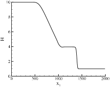
Figure 7: 1D dam break problem, solved with first order FVEG method. Left: solution with entropy fix from [LukacovaTadmor2009] Right: solution with new entropy fix

In Fig. 7 we compare the results of the entropy stable scheme from [LukacovaTadmor2009] and our new approach. They both clearly solve the entropy problem, with a slight advantage of the scheme by Lukáčová and Tadmor. However, as we previously pointed out, the new method is more efficient. Compared to the scheme without any entropy fix, the new one took only about 2% extra time, whereas the approach from [LukacovaTadmor2009] needs about 8% more computational time. As the new scheme is also suitable for computations including dry areas, we chose it for all the numerical experiments in Section 5.

4 Dry Bed Modifications

To extend our schemes to computations including dry beds, we have to guarantee two properties: the positivity of the water height, and the well-balancing under the presence of dry areas. In literature, this is mainly achieved by two basic ingredients: a positivity preserving reconstruction and an additional time step constraint. Examples can be found in [AudusseBouchutBristeauEtAl2004, KurganovPetrova2007, RicchiutoBollermann2009].

For the FVEG schemes, these measures fall short of the aims. The additional predictor step via the evolution operator prevents a direct proof of a positivity property. One reason for this is the extended stencil: the flux over an edge is computed using more cells than the direct neighbours (see Fig. 1 and 3). Another problem is the complex evaluation of the operators and with them the flux which makes an analysis of the positivity at least challenging if not impossible.

Regarding the well-balancing, a sophisticated reconstruction is not enough. From (19) it is obvious that the reconstruction does not directly affect the balancing of flux and source terms. The core of the problem is that the lake at rest described in (12) changes to

$${\vec{v}}=(0,0)^{T}\text{ and }H(\vec{x})=\begin{cases}H_{0}&\text{$h({\vec{x}})>0$}\\ b({\vec{x}})&\text{else}\end{cases}$$ (40)

if dry areas are included. Thus for our schemes, we have to find evolution values for the water and bottom height that can handle properly the occurrence of this situation, i.e. which avoid the generation of spurious waves at the shoreline.

In this section, we will present an alternative approach to ensure the positivity of the water height as well as modifications of the finite volume update and the evolution operator to ensure the well-balancing property. We make sure that the changes do not affect the scheme away from dry regions.

4.1 A General Positivity Preserving FV Update

For the derivation of a positivity preserving scheme, we study the first component of the finite volume update (20)

$$h_{i}^{n+1}=h_{i}^{n}-\frac{\Delta t}{\Delta x}\sum_{E,E\subset\partial C_{i}}\boldsymbol{\mathcal{H}}_{E}$$ (41)

where

$$\boldsymbol{\mathcal{H}}_{E}:=\boldsymbol{\mathcal{F}}_{E}^{h}$$ (42)

is the first component of the flux vector $\boldsymbol{\mathcal{F}}_{E}$. In the following, we will modify the flux $\boldsymbol{\mathcal{H}}_{E}$ in order to guarantee positive water height. The technique presented here is applicable to arbitrary finite volume fluxes, and the FVEG flux given in (18) below is only a special case within this framework.

The basic idea of our method is to cut off the outgoing fluxes as soon as all water which has been contained in the cell at the beginning of the time step has left the cell via the outgoing fluxes. We will call this time the draining time. For convenience, we will later rewrite this as a reduced time step $\Delta t_{E}$ on these edges, but in fact the finite volume update will always advance the solution by one global time step $\Delta t$.

Thus our first step is to separate the fluxes contributing to the outflow off a cell $C$ from those contributing to the inflow by setting

$$\boldsymbol{\mathcal{H}}^{+}_{E} :=\max\left\{\boldsymbol{\mathcal{H}}_{E},0\right\}$$ (43)

$$\boldsymbol{\mathcal{H}}^{-}_{E} :=\min\left\{\boldsymbol{\mathcal{H}}_{E},0\right\}.$$ (44)

This allows us to rewrite the update (41) as

$$h_{i}^{n+1}=h_{i}^{n}\;-\;\underbrace{\frac{\Delta t}{\Delta x}\sum_{E,E\subset\partial C_{i}}\boldsymbol{\mathcal{H}}_{E}^{+}}_{\text{outflow}}\;-\;\underbrace{\frac{\Delta t}{\Delta x}\sum_{E,E\subset\partial C_{i}}\boldsymbol{\mathcal{H}}_{E}^{-}}_{\text{inflow}}.$$ (45)

Now we introduce the draining time by

$$\Delta t_{C_{i},\text{drain}}:=\frac{\Delta x\,h_{i}^{n}}{\sum_{E,E\subset\partial C_{i}}\boldsymbol{\mathcal{H}}_{E}^{+}}.$$ (46)

Once again, at time $t^{n}+\Delta t_{C_{i},\text{drain}}$ all water which was originally contained in cell $C_{i}$ has flown out, so

$$h_{i}^{n}\;-\;\underbrace{\frac{\Delta t_{C_{i},\text{drain}}}{\Delta x}\sum_{E,E\subset\partial C_{i}}\boldsymbol{\mathcal{H}}_{E}^{+}}_{\text{outflow}}=0.$$ (47)

Suppose now that $\Delta t_{C_{i},\text{drain}}<\Delta t$. For $t\in[t^{n}+\Delta t_{C_{i},\text{drain}}\,,\,t^{n+1}]$, no more water can leave the cell, at least not water which was originally contained in cell $C_{i}$. Therefore we assume that there is no outgoing flux for times beyond the draining time, and introduce the cut-off flux $\widetilde{\boldsymbol{\mathcal{H}}}_{E}^{+}$ by

$$\widetilde{\boldsymbol{\mathcal{H}}}_{E}^{+}(t):=\begin{cases}\boldsymbol{\mathcal{H}}_{E}^{+}({\mathbf{u}}^{n})&\text{ for}\;\;t^{n}\;\leq\;t\;<\;t^{n}+\Delta t_{C_{i},\text{drain}}\\ \quad 0&\text{ for}\;\;t\;>\;t^{n}+\Delta t_{C_{i},\text{drain}}\end{cases}$$ (48)

Now we integrate the draining flux in time and obtain the cut-off (or draining) finite volume flux

$$\Delta t\,\boldsymbol{\mathcal{H}}^{+}_{E,\text{drain}}({\mathbf{u}}^{n}):=\int_{t^{n}}^{t^{n+1}}\widetilde{\boldsymbol{\mathcal{H}}}_{E}^{+}(t)dt=\int_{t^{n}}^{t^{n}+\Delta t_{C_{i},\text{drain}}}\boldsymbol{\mathcal{H}}_{E}^{+}({\mathbf{u}}^{n})dt=\Delta t_{C_{i},\text{drain}}\boldsymbol{\mathcal{H}}_{E}^{+}({\mathbf{u}}^{n}).$$ (49)

Before introducing the positivity-preserving modification of the finite volume scheme (20), we rewrite the cut-off in the flux as a local cut-off in the time step. This cut-off time step is defined for each edge $E$ and takes into account the upwind cell $C^{-}(E)$:

$$\Delta t_{E}:=\min\left(\Delta t,\Delta t_{C^{-}(E),\text{drain}}\right)$$ (50)

Now we replace the finite volume flux $\boldsymbol{\mathcal{H}}$ in (20) by the cut-off finite volume flux defined in (49). Using (50), this leads to the modified general update (20)

$${\mathbf{u}}_{i}^{n+1}={\mathbf{u}}_{i}^{n}-\frac{1}{\Delta x}\sum_{E,E\subset\partial C_{i}}\Delta t_{E}\boldsymbol{\mathcal{F}}_{E}.$$ (51)

Theorem 4.1.

Assume we have a conservative finite volume scheme for the solution of the shallow water equations that can be written in the form (20). Then the modified finite volume scheme (51) with locally cut-off flux (49)) (respectively locally cut-off time step (50)) is positivity preserving.

Proof 4.2.

From the first component of (51), combined with definitions (50) of the cut-off time step $\Delta t_{E}$ and (46) of the draining time $\Delta t_{C_{i},\text{drain}}$, the water height at the new time step can be bounded as follows:

$$h_{i}^{n+1} \;=\;\;\;h_{i}^{n}\;\;-\;\sum_{E,E\subset\partial C_{i}}\frac{\Delta t_{E}}{\Delta x}\;\left(\boldsymbol{\mathcal{H}}_{E}^{+}+\boldsymbol{\mathcal{H}}_{E}^{-}\right)$$

$$\;\geq\;\;\;h_{i}^{n}\;\;-\;\sum_{E,E\subset\partial C_{i}}\frac{\Delta t_{E}}{\Delta x}\;\boldsymbol{\mathcal{H}}_{E}^{+}$$

$$\;\geq\;\;\;h_{i}^{n}\;\;-\;\sum_{E,E\subset\partial C_{i}}\frac{\Delta t_{C^{-}(E),\text{drain}}}{\Delta x}\boldsymbol{\mathcal{H}}_{E}^{+}$$

$$\;=\;\;\;h_{i}^{n}\;\;-\;\frac{\Delta t_{C_{i},\text{drain}}}{\Delta x}\sum_{E,E\subset\partial C_{i}}\boldsymbol{\mathcal{H}}_{E}^{+}$$

$$\;=\;\;\;0$$

Remark 4.3.

The time step $\Delta t_{E}$ used in the new finite volume update (51) and defined in (50) might seem to be local for each edge. We would like to stress, however, that the finite volume scheme (51) still advances the solution by one and the same global time step $\Delta t$. The apparent contradiction is resolved by considering equation (49): the time-integral of the flux is still over the global interval $[t^{n},t^{n+1}]$. However, the flux $\boldsymbol{\mathcal{H}}^{+}_{E,\text{drain}}$ is cut-off in the presence of vacuum, see (48).

4.2 Well-balancing at the Shoreline: the Finite Volume Update

In the derivation of the positivity preserving finite volume update, we so far neglected the source term. Its introduction to the new scheme (51) rises the question which time step should be used for the source term. To maintain the well-balancing, the source term and the gravity driven parts of the flux must be multiplied with the same time step. This is in contradiction to the definition of $\Delta t_{E}$, which may change for different edges of the same cell. On the other hand, the reduced time step is not necessary for the momentum equations. We therefore shift the gravity driven components of $\boldsymbol{\mathcal{F}}$ into the source term, i.e. we define

$$\boldsymbol{\mathcal{F}}^{*}({\mathbf{u}}):=\begin{pmatrix}hv_{1}&hv_{2}\\ hv_{1}^{2}&hv_{1}v_{2}\\ hv_{1}v_{2}&hv_{2}^{2}\end{pmatrix}\text{ and }\boldsymbol{\mathcal{S}}^{*}({\mathbf{u}},{\vec{x}}):=gh\begin{pmatrix}0\\ \frac{\partial H(\vec{x})}{\partial x_{1}}\\ \frac{\partial H(\vec{x})}{\partial x_{2}}\end{pmatrix}.$$ (52)

By replacing $\boldsymbol{\mathcal{F}}$ with $\boldsymbol{\mathcal{F}}^{*}$ in (18) and changing (19) to

$$\boldsymbol{\mathcal{S}}^{*}_{i}:=g\sum_{j=1}^{3}\alpha_{j}\begin{pmatrix}0\\ \frac{1}{2}(\hat{h}_{j}^{r}+\hat{h}_{j}^{l})(H^{r}_{j}-H_{j}^{l})\\ \frac{1}{2}(\hat{h}_{j}^{t}+\hat{h}_{j}^{b})(H_{j}^{t}-H_{j}^{b})\end{pmatrix}$$ (53)

we can rewrite (20) as

$${\mathbf{u}}_{i}^{n+1}={\mathbf{u}}_{i}^{n}-\frac{1}{\Delta x}\left[\left(\sum_{E,E\subset\partial C_{i}}\Delta t_{E}\boldsymbol{\mathcal{F}}^{*}_{E}\right)+\Delta t\boldsymbol{\mathcal{S}}^{*}_{i}\right].$$ (54)

This formulation ensures the well-balancing of the scheme even in the case of modified local time steps. Away from the shoreline we have $\Delta t_{E}=\Delta t\;\forall E$ and (54) equals the original update (20).

Remark 4.4.

The rearrangement of the advective and gravity driven parts of the equations in (52) is independent of the scheme. Thus in principle, every finite volume scheme can be reformulated as in (54). To obtain a well-balanced scheme, we only need a discretisation of $\boldsymbol{\mathcal{S}}^{*}$ analogously to (53) that preserves the lake at rest solution in the presence of dry boundaries.

4.3 Well-balancing at the Shoreline: the Evolution Operator

The lake at rest situation with dry beds described in (40) is only preserved if the numerical flux and source terms in (53) are exactly balanced, or equivalently if the evolution operators reproduce the lake at rest. This is not necessarily the case if the stencil of a quadrature point contains dry cells, as is demonstrated in Fig. 8. If $b_{i}>H_{o}$ for a cell in the stencil, the resulting bottom value from (38) can be higher than the free surface in the wet cells. Using the approximate evolution operators (30) and (33), it is easy to see that in the lake at rest case the evolved water height is also positive, leading to an even higher free surface at the quadrature point.

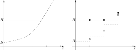
Figure 8: Lake at rest with dry boundaries. Solid line: free surface, dashed line: bottom topography, filled circles: $H$ at evolution points, empty circles: $B$ at evolution points. Left: Real situation. Right: Numerical Representation with evolution values.

In this case the combined flux and source term $\boldsymbol{\mathcal{S}}^{*}$ from (53) does not vanish anymore and introduces unphysical waves starting from the dry boundary.

To avoid the creation of these waves, we modify the data used for the predictor step at the interface. First, we replace the stencil $S_{k}$ by $S^{*}_{k}$ defined as

$$S^{*}_{k}:=\{C_{i}|C_{i}\in S_{k}\wedge h_{i}>0\}$$ (55)

which allows us to determine the maximal free surface level at ${\vec{x}}_{k}$ as

$$\bar{H}_{k}=\max_{S^{*}_{k}}(H_{i}).$$ (56)

Now in (37) and for the evaluation of the evolution operators we set

$$(H,b,{\vec{v}})_{i}=(\bar{H}_{k},\bar{H}_{k},0)\quad\text{ if }C_{i}\notin S^{*}_{k}\wedge b_{i}>\bar{H}_{k}.$$ (57)

In all other cases, we leave the values unchanged. The modification, which is illustrated in Fig. 9, ensures that the free surface is correctly represented in the source term computation (53). We also avoid an unphysical flooding of mounting slopes. In [BrufauGarcia-Navarro2003, RicchiutoBollermann2009] a similar technique is used on triangles.

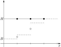
Figure 9: Lake at rest with dry boundaries, modification (57) for computation of evolution values. Symbols like in Fig. 8

Finally, even in the presence of wet, but nearly dry cells in the stencil, the expressions for $h(P)$ in (30) and (33) can become negative if $h_{i}$ is small in the surrounding cells. This cannot necessarily be cured by a smaller time step, as substantial parts of the expressions do not depend on $\Delta t$. With this restriction in mind, we propose the simplest solution: Whenever we have $h(P)<0$, we set $h(P)=v_{1}(P)=v_{2}(P)=0$.

4.4 Treatment of Nearly Dry Cells

In our schemes, we consider a cell $C_{i}$ to be dry when $h_{i}<\varepsilon_{H}$, where we have chosen $\varepsilon_{h}=10^{-8}$. In dry cells we set $h_{i}=u_{i}=v_{i}=0$. A well known problem occurs when $h_{i}$ is close to that value: the velocity $v=hv/h$ can become singular due to small numerical errors in the conserved variables. This leads to very small time steps which in the end can basically stop the computation. This problem has been discussed e.g. in [KurganovPetrova2007, RicchiutoBollermann2009], where different strategies have been proposed. In [KurganovPetrova2007], Kurganov and Petrova propose to de-singularise $v$ by multiplying it with a certain factor $f<1$ whenever $h$ falls below a certain threshold $\varepsilon_{v}$. In [RicchiutoBollermann2009], the authors just set $v=0$ whenever $h<\varepsilon_{v}$.

In this work, we use a different approach. As the solution at the dry boundary is always a rarefaction wave, the flow velocity will grow smoothly when water floods formerly dry areas. We will therefore limit the velocity in nearly dry regions depending on the velocity in flooded areas. We define the reference speed

$$v_{ref}:=\max_{i:h_{i}>\varepsilon_{v}}\|{\vec{v}}\|_{2}$$ (58)

where

$$\varepsilon_{v}=\frac{\Delta x}{L_{ref}},\quad L_{ref}:=\max_{i,j}\|{\vec{x}}_{i}-{\vec{x}}_{j}\|_{\infty}.$$ (59)

Whenever we have $h_{i}<\varepsilon_{v}$ and $\|{\vec{v}}_{i}\|>v_{ref}$, we set the new velocity to

$$v^{*}_{i}=v_{ref}\left(2-\frac{v_{ref}}{\|{\vec{v}}_{i}\|}\right),$$ (60)

such that $\|{\vec{v}}\|$ is smoothly limited to a value between $v_{ref}$ and $2v_{ref}$. The velocity components in $C_{i}$ are then defined as

$${\vec{v}}_{i}=v^{*}_{i}\vec{d}$$ (61)

with $\vec{d}$ the unit vector pointing in the same direction as the vector of discharge $(hv_{1},hv_{2})^{T}$. This approach appears us to be a better representation of the physics of the flow, as the velocity at the front is not necessarily vanishing.

4.5 The FVEG Algorithm

Before summarising the whole FVEG algorithm, we will spend a few words on the reconstruction needed to evaluate the evolution operators for piecewise linear data (33) – (35). As the operators are computed from the primitive variables ${\mathbf{w}}$, these are a natural choice for the reconstruction $R_{\Delta x}$. Thus in each cell we need the linear function

$$R_{\Delta x}({\mathbf{w}}_{i})({\vec{x}})_{|C_{i}}:=\tilde{\mathbf{w}}_{i}+\nabla{\mathbf{w}}_{i}\cdot({\vec{x}}-{\vec{x}}_{i})+({\mathbf{w}}_{i})_{x_{1}x_{2}}({\vec{x}}-{\vec{x}}_{i})_{1}({\vec{x}}-{\vec{x}}_{i})_{2}.$$ (62)

The derivatives $({\mathbf{w}}_{i})_{x_{1}},({\mathbf{w}}_{i})_{x_{2}}$ and $({\mathbf{w}}_{i})_{x_{1}x_{2}}$ are computed from the slopes between cell averages, cf. [LukacovaSaibertovaWarnecke2002]. In this paper, we use the continuous, piecewise bilinear recovery described in [LukacovaNoelleKraft2007] without any limiters. The piecewise bilinear functions are uniquely defined by the averages at the cell corners, which are already computed for the evaluation of the evolution operators, see (37). Then the $\tilde{\mathbf{w}}$ from (62) is exactly the average of the averages at the cell corners, thus the resulting reconstruction is not necessarily conservative. We will therefore use the combined evolution operator

$${\mathbf{E}}({\mathbf{W}}):={\mathbf{E}}^{\text{bilin}}(R_{\Delta x}({\mathbf{W}}))+{\mathbf{E}}^{\text{const}}({\mathbf{W}}-\tilde{\mathbf{W}}),$$ (63)

where the first order correction ${\mathbf{E}}^{\text{const}}({\mathbf{W}}-\tilde{\mathbf{W}})$ is necessary for stability, see [LukacovaMortonWarnecke2004] for an in-depth discussion of this issue.

Although the conservative correction introduces some oscillations at steep fronts, the piecewise bilinear reconstruction has a clear advantage in the vicinity of dry areas. As the averaged water height at the cell corners is non-negative via eqs. (55) – (57), the reconstruction is also non-negative by design. In dry cells, we set

$${\mathbf{w}}_{x_{1}}={\mathbf{w}}_{x_{2}}={\mathbf{w}}_{x_{1}x_{2}}=0\text{ if }h_{i}=0.$$ (64)

We refer to [LukacovaNoelleKraft2007, LukacovaSaibertovaWarnecke2002] for further details concerning the reconstruction strategy.

The complete algorithm now reads as follows:

Algorithm 1.

1. From given conservative data ${\mathbf{u}}_{i}^{n}$ and $b_{i}$ at time $t^{n}$, compute the nonconservative variables $H_{i}^{n},v_{1,i}^{n},v^{n}_{2,i}$.

2. apply the reconstruction operator $R_{\Delta x}$ to $H_{i}^{n},v_{1,i}^{n},v^{n}_{2,i}$ and $b_{i}$.

3. compute the evolution operators

4. evaluate the advection fluxes $\boldsymbol{\mathcal{F}}^{*}_{E}$ from (52)

5. compute the gravity driven flux and source terms $\boldsymbol{\mathcal{S}}^{*}_{i}$ from (53)

6. perform the finite volume update (54)

We will finish the section by a proof of the well-balancing property of the scheme.

Theorem 4.5.

Suppose that we have a numerical solution respecting the lake at rest solution (40) with dry boundaries. Then the FVEG scheme (54) together with the modifications described in Section 4.3 preserves this state.

Proof 4.6.

For the lake at rest state with ${\vec{v}}=(0,0)^{T}$, the advective parts of the fluxes $\boldsymbol{\mathcal{F}}$ defined in (2) and $\boldsymbol{\mathcal{F}}^{*}$ defined in (52) are all zero. Thus for all edges we have $\Delta t_{E}=\Delta t$ and the original finite volume update (20) and the modified update (54) are the same. Then Theorem 2.1 from [LukacovaNoelleKraft2007] states that the scheme is well-balanced provided that the predicted point values used for the flux evaluation also satisfy the lake at rest situation.

We will now show that all data used for the reconstruction and for the evaluation of the predictor step satisfies the requirements of Theorem 3.1 from [LukacovaNoelleKraft2007]. From definitions (55) and (56) we see that for all evolution points the averaged free surface is computed as $H_{0}$, which is the free surface level in all flooded cells. As all velocities are zero by (40) respectively (57), the averaging also returns zero. Finally, the reconstruction procedure is based on the averaged point values and therefore in all flooded cells we have ${\mathbf{w}}_{x_{1}}={\mathbf{w}}_{x_{2}}={\mathbf{w}}_{x_{1}x_{2}}=0$. In dry cells we have the same result by definition (64). Thus we can apply Theorem 3.1 from [LukacovaNoelleKraft2007] and this concludes our proof.

5 Numerical Results

5.1 Dam Break over Dry Bed

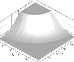
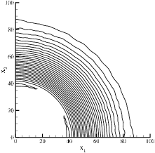
Figure 10: Circular dam break over dry bed, solution at t=1.75s. Left: 3D view. Right: 30 contour lines between $H=10.2$ and $H=0.2$

This is a classical test case where we simulate the complete break of a circular dam separating a basin filled with water from a dry area. The computational domain is $[0,100]^{2}$ and we set $\Delta x=1$, the water filled basin is located at $r=\|{\vec{x}}\|\leq 60$. In the basin we set $H_{0}=10$ and elsewhere $H_{0}=0$ and the initial velocity is ${\vec{v}}_{0}=(0,0)^{tr}$ in the whole domain. Reference solutions can be found in [RicchiutoBollermann2009, Seaid2004, AlcrudoGarcia-Navarro1993].

In Fig. 10, we see a 3D view and contour lines of the water height, Fig. 11 shows the water height and velocity at different lines through the domain. The resulting rarefaction wave is almost perfectly symmetric, the oscillation due to the reconstruction strategy is restricted to three percent of the water height (we have $\max_{i}H_{i}=10.269$). We see a small bump at the drying wetting front, but the front position and velocities are well represented. Thanks to the new entropy fix, there is no unphysical shock visible in the transcritical region.

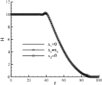
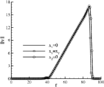
Figure 11: Circular dam break over dry bed, solution at t=1.75s with $r=\|{\vec{x}}\|_{2}$. Left: free surface. Right: velocity

5.2 Wetting/Drying on a Sloping Shore

This test case was proposed by Synolakis in [Synolakis1987] and computed in e.g. [RicchiutoBollermann2009, MarcheBonnetonFabrieEtAl2007]. It describes the run-up and reflection of a wave on a mounting slope, with the initial solution given as

$$H_{0}({\vec{x}})=\max(f,b({\vec{x}})),\quad{\vec{v}}_{0}({\vec{x}})=\left(\sqrt{\frac{g}{D}}H_{0}(\vec{x}),0\right)^{T}$$ (65)

where

$$f({\vec{x}})=D+\delta\operatorname{sech}^{2}(\gamma(x_{1}-x_{a})).$$ (66)

As in [RicchiutoBollermann2009, MarcheBonnetonFabrieEtAl2007], we set $D=1,\delta=0.019$ and

$$\gamma=\sqrt{\frac{3\delta}{4D}},\qquad x_{a}=\sqrt{\frac{4D}{3\delta}}\mathrm{arcosh}\left(\sqrt{20}\right).$$ (67)

For the bottom topography we have

$$b({\vec{x}})=b(x_{1})=\begin{cases}0&\text{$x_{1}<2x_{a}$}\\ \dfrac{x_{1}-2x_{a}}{19.85}&\text{else.}\end{cases}$$ (68)

The computational domain is $\Omega=[0,80]\times[0,2]$ and the grid size $\Delta x=0.04$. We prescribe open boundary conditions in $x_{1}$ direction and periodic ones in $x_{2}$ direction.

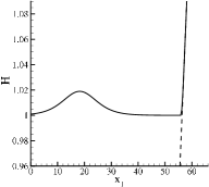
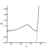
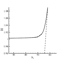
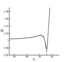
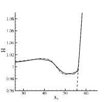
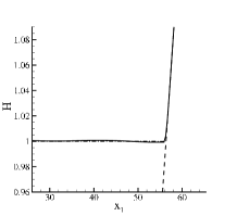
Figure 12: Drying/wetting on a sloping shore, free surface. Solid line: numerical results. Dashed-dotted line: Analytical result described in [Synolakis1987]. Dashed line: bottom height. From top left to bottom right: Solutions at times $t=0$, $t=9$, $t=17$, $t=23$, $t=28$ and $t=80$.

In Fig. 12 we present the water height during the run-up and drying process together with the analytical solution. Details on how to obtain the analytical solution can be found in [Synolakis1986, Section 3.5.2]. At time $t=9$, the wave has almost reached the shoreline, and shortly after, at $t=17$, the wave reaches the maximal run-up on the shore and the drying process starts. During the run-up, the agreement with the analytical solution is excellent. The drying process is reproduced very accurate, too, although compared to the run-up process, there are small deviations between numerical and analytical solution with respect to the minimum of the water height at $t=23$. At $t=28$, where the reflected wave starts leaving the domain, these deviations persist, but stay very small. During the whole simulation, no oscillations or other perturbations at the wetting/drying front are visible, demonstrating the well-balancing capabilities of the scheme. The scheme also returns quickly to the lake at rest solution presented in the last picture ($t=80$). where the water surface is almost flat. All in all, the results are very satisfying and compare well to the other numerical solutions presented in [RicchiutoBollermann2009, MarcheBonnetonFabrieEtAl2007].

5.3 Vacuum occurrence by a double rarefaction wave over a step

To test how the scheme handles the drying of formerly flooded areas, we compute a test case proposed in [GallouetHerardSeguin2003]. It describes two separating waves over a non-flat bottom. The computational domain is a pseudo-1D channel given as $\Omega=[0,25]\times[0,0.5]$. We set the initial free surface height to $H^{0}=10$ and the discharge and bottom topography to

$$hv_{1}({\vec{x}},0)=\begin{cases}350&\text{if $x_{1}>50/3$}\\ -350&\text{else}\end{cases}\qquad b({\vec{x}})=\begin{cases}1&\text{if $25/3<x_{1}<25/2$}\\ 0&\text{else}\end{cases}.$$ (69)

Like in [GallouetHerardSeguin2003], the computation is performed on a grid with 300 grid cells in $x_{1}$ direction.

In Fig. 13, we show the free surface and the discharge of the solution at different times $t$. At time $t=0.5$, several waves have arisen from the interaction of the supersonic flow with the bottom topography. Due to the reconstruction strategy described in Sec. 4.5, the rarefaction waves are smoothed out at the bottom and show small oscillations at the top. However, for the following times we see an accurate representation of the waves flowing over the hump ($t=0.25$) and leaving the domain ($t=0.45,0.65$). No spurious modes are introduced during the drying process, neither in the flat region nor at the edges of the hump.

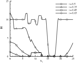
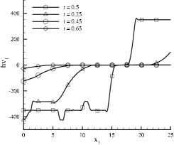
Figure 13: Vacuum occurrence, solution at different times. Left: free surface. Right: discharge.

5.4 Thacker’s Periodic Solutions

We present two exact solutions of (1) proposed by Thacker in [Thacker1981]. They both describe oscillations of a free surface in a parabolic basin with a free shoreline. The basin is defined as

$$b(\vec{x})=b(r_{c})=-H_{0}\left(1-\frac{r_{c}^{2}}{a^{2}}\right).$$ (70)

$r_{c}$ defines the distance from the basin’s centre, $H_{0}$ the height of the centre and $a$ is a parameter. We will define two functions $f(\vec{x},t)$ that describe solutions of (1) with $h(\vec{x},t)=\max(f(\vec{x},t)-b(\vec{x}),0)$. Both test cases will be computed on the domain $\Omega=[-2,2]^{2}$. The presented results have been performed with a grid size of $\Delta x=0.4$. Reference solutions can be found in [RicchiutoBollermann2009, RicchiutoBollermann2008, MarcheBonnetonFabrieEtAl2007].

5.4.1 Thacker’s Curved Solution

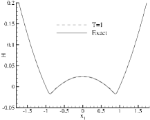
Figure 14: Thackers curved solutions. Left: $t=T$. Right: $t=3T$

The first function results in a curved oscillation over $b$, it reads

$$f(r_{c},t)=H_{0}\left(-1+\frac{\sqrt{1-A^{2}}}{1-A\cos(\omega t)}-\frac{r_{c}^{2}}{a^{2}}\left(1-\frac{1-A^{2}}{(1-A\cos(\omega t))^{2}}\right)\right).$$ (71)

Here, $\omega=\sqrt{8gH_{0}/a^{2}}$ is the frequency and for a given $r_{0}>0$, $A$ is the shape parameter

$$A=\frac{a^{2}-r_{0}^{2}}{a^{2}+r_{0}^{2}}.$$

For the computation we set $a=1$, $H_{0}=0.1$ and $r_{0}=0.8$, which results in an oscillating period of $T\approx 2.22$. The initial velocity is set to ${\vec{v}}_{0}=(0,0)^{tr}$.

# cells	$L^{\infty}$	EOC	$L^{1}$	EOC	$L^{2}$	EOC
25 $\times$ 25	9.8038e-03		1.4526e-02		9.2884e-03
50 $\times$50	3.6191e-03	1.44	3.9038e-03	1.90	2.7762e-03	1.74
100 $\times$100	1.5252e-03	1.25	1.3127e-03	1.57	9.5937e-04	1.53
200 $\times$200	1.1820e-03	0.37	4.6649e-04	1.49	3.8549e-04	1.32
400 $\times$400	5.3221e-04	1.15	1.7806e-04	1.39	1.4907e-04	1.37

Table 1: Experimental order of convergence (EOC) for Thackers curved solution. Error in water height in different norms.

5.4.2 Thacker’s Planar Solution

The second solution is a planar surface rotating around the basin. The corresponding function is

$$f(\vec{x},t)=\frac{\eta H_{0}}{a^{2}}(-\eta+2(\vec{x}-\vec{x}_{C})\cdot(\cos(\omega t),\sin(\omega t))^{tr})$$ (72)

with $\omega=\sqrt{2gH_{0}/a^{2}}$ the frequency and $\eta$ another parameter. Here, we set $a=1$, $H_{0}=0.1$ and $\eta=0.5$. The resulting period is then $T\approx 4.44$. The initial velocity in the wetted domain is given as ${\vec{v}}_{0}=(0,\eta\omega)^{tr}$.

# cells	$L^{\infty}$	EOC	$L^{1}$	EOC	$L^{2}$	EOC
25 $\times$ 25	3.3855e-02		4.6507e-02		2.7148e-02
50 $\times$50	1.7455e-02	0.96	1.8179e-02	1.36	1.1660e-02	1.22
100 $\times$100	1.0543e-02	0.73	1.0486e-02	0.79	6.6938e-03	0.80
200 $\times$200	8.2376e-03	0.36	8.3640e-03	0.33	5.4658e-03	0.29
400 $\times$400	7.1238e-03	0.21	7.8559e-03	0.09	5.1747e-03	0.08

Table 2: Experimental order of convergence (EOC) for Thackers planar solution. Error in water height in different norms.

We present the water height after one and three oscillations along the line $x_{2}=0$ in Fig. 14 for the curved solution and in Fig. 15 for the planar solution. The exact solution is very well reproduced, independent of the shape of the initial solution. We can see a slight smearing after three periods for the curved solution, where the maximum value at the centre is reduced and the drying/wetting interface has been pushed outward. Similarly, the interface of the planar solution has also moved a little bit inwards at $t=3T$. Again, for both solutions there is no production of spurious waves at the dry boundary.

In Tables 1 and 2 we present a convergence study for the two test cases. The experimental order of convergence for the curved solution is well better than one, which meets our expectations. The errors are slightly better than in [RicchiutoBollermann2008].

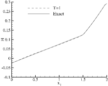
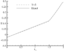
Figure 15: Thackers planar solutions. Left: $t=T$. Right: $t=3T$

For the planar solution, however, the order quickly drops to zero. The problem seems to raise from the boundary of the wetted domain, where we have supersonic velocities tangential to the bottom slope. So the problem might be related to the evolution operators, as they produce inexact solutions in other supersonic situations as well, see the discussion in Section 3.4 and 6.

5.5 Wave Run-up on a Conical Island

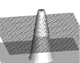
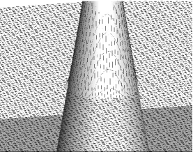
Figure 16: Circular island, lake at rest situation at $t=5$. Left: whole domain. Right: zoom on island.

In this case we simulate the run-up of a solitary wave over a conical island. It has been performed experimentally at the U.S. Army Engineer Waterways Experiment Station, see [BriggsSynolakisHarkinsEtAl1995, tsunami]. The computational domain is $\Omega=[0,25]\times[0,30]$ and we set $\Delta x=0.2$. The centre of the island is located at ${\vec{x}}_{C}=(12.5,15)$ and with $r=\|{\vec{x}}-{\vec{x}}_{C}\|$ its shape is given by

$$b(r)=\begin{cases}0.625&\text{$r\leq 1.1$}\\ (3.6-r)/4&\text{$r\leq 3.6$}\\ 0&\text{else.}\end{cases}$$ (73)

The initial free surface is given by $H_{0}=0.32$. We start by giving an example of the well-balancing capabilities of the scheme and compute the lake at rest situation until $t=5$. The results are shown in Fig. 16. The lake at rest is perfectly preserved, which is confirmed by the errors given in Table 3. For all the 3D views of this example, the vertical axis representing the free surface was scaled by a factor of 25 to emphasise the results.

	$L^{\infty}$	$L^{1}$	$L^{2}$
$e_{H}$	4.44089e-16	6.50361e-14	3.14147e-15
$e_{v_{1}}$	2.69215e-15	2.53222e-13	1.24917e-14
$e_{v_{2}}$	2.92617e-15	2.73056e-13	1.33148e-14

Table 3: Lake at rest around a conical island. Errors at $t=5$.

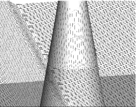
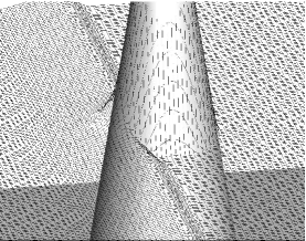
Figure 17: Run-up on a circular island. Left: wave approaching island, $t=7.9$. Right: run-up at front of the island, $t=9.1$.

We now compute the actual wave where at time $t=0$ a wave enters the computational domain at $x_{1}=0$. The height of the wave is given by

$$H(0,y,t)=H_{0}+\alpha H_{0}\left(\frac{1}{\cosh(\xi\sqrt{gH_{0}/L}(t-3.5)}\right)^{2}$$

with $L=15$, $\alpha=0.1$ and $\xi=\sqrt{3\alpha(1+\alpha)L^{2}/(4H_{0}^{2})}$, cf. [HubbardDodd2002, MarcheBonnetonFabrieEtAl2007].

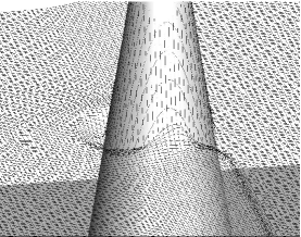
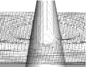
Figure 18: Run-up on a circular island. Left: lateral run-up, $t=10.7$. Right: symmetric waves around the island, $t=12.1$.

We present 3D views of the solution in Fig. 17, 18 and 19. Fig. 17 shows the wave approaching the island and the instant of its maximal run-up. Here, as in all the following figures, the region in front of the wave remains completely unaffected, once again confirming the well-balancing of the scheme. Due to the run-up, the wave is slowed down at the island, finally resulting in a reflection of the wave presented in Fig. 18. This leads to the formation of two symmetric waves surrounding the island with a noticeable run-up also on the sides of the island. Away from the island, we observe the circular reflected wave approaching the boundaries of the computational domain. Behind the island, the lateral waves reunite and produce a second peak in the run-up on the lee side of the island, see Fig. 19. Finally, the wave leaves the domain and the surface returns to the lake at rest, as shown in the last picture.

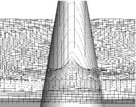
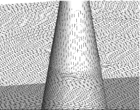
Figure 19: Run-up on a circular island. Left: run-up behind the island, $t=13.7$. Right: reestablished lake at rest at $t=40$.

Figure 20: Run-up on a circular island. Time variation of the free surface $\eta=H-H_{0}$ at wave gages 6, 9, 16, and 22 of experiment from [BriggsSynolakisHarkinsEtAl1995]. Dotted line: experimental data from [tsunami]. Solid line: FVEG scheme. Dashed-dotted line: RD scheme from [RicchiutoBollermann2009]

Figure 21: Run-up on a circular island. Time variation of the free surface $\eta=H-H_{0}$ at wave gages 6, 9, 16, and 22 of experiment from [BriggsSynolakisHarkinsEtAl1995], convergence of FVEG scheme. Dashed-dotted line: $\Delta x=1/8$ Dotted line: $\Delta x=1/16$ Solid line: $\Delta x=1/32$

Moreover we show the evolution of the free surface at chosen points in Fig. 20. The position of the gages is given by ${\vec{x}}_{3}=(6.36,14.25)$, ${\vec{x}}_{6}=(8.9,15)$, ${\vec{x}}_{9}=(9.9,15)$, ${\vec{x}}_{16}=(12.5,12.42)$ and ${\vec{x}}_{22}=(15.1,15)$. For comparison we also display the measured data obtained from [tsunami] as well as the results from the residual distribution (RD) scheme presented in [RicchiutoBollermann2009], which have been computed on a comparable grid. Both numerical schemes produce steeper wave fronts than the experiment, which results from the lack of dissipation in the shallow water model. The FVEG scheme shows a stronger steepening than the RD scheme, and also predicts slightly higher waves at all gages. At gages 3 and 6, the run-down process is pretty similar with both schemes, while the FVEG scheme returns quicker to a constant water height. Both schemes produce less accurate results at gage 9. The FVEG line is shifted to the upper left, thus resulting in a less pronounced run-down and again it returns quickly to a constant height. The RD scheme provides smoother results with a better approximation of the maximal run-down, but stays below the original water height for a longer period. At gage 16, the FVEG scheme gives a quite accurate representation of the wave, where the RD scheme introduces an undershoot after the first wave. At the last gage, the graph of the FVEG scheme is similar to the measurement, but somewhat shifted to the upper right. This is probably due to the over-prediction of the maximal wave height. The RD schemes gives a better approximation of the maximal height, but the following graph is smoothed out stronger. Finally, in Fig. 21, we present solutions at the gages for different grid resolutions, computed with the FVEG scheme. We can clearly see that the scheme converges. The steepening of the fronts becomes more pronounced and the perturbations during the run-down vanish on the finer grids. However, the main features are already captured on the relatively coarse grid used for the simulation in Fig. 20. All in all, the FVEG scheme produces a good reproduction of the wave, and the results are clearly competitive to other numerical schemes like the ones presented in [HubbardDodd2002, RicchiutoBollermann2009].

6 Conclusions and Outlook

We presented an approach to ensure positivity of the water height for general finite volume schemes without affecting the global time step. This was achieved by limiting the outgoing fluxes of a cell whenever they would create negative water height. Physically, this corresponds to the absence of fluxes in the presence of vacuum. A splitting of advective and gravity driven parts of the flux preserved the well-balancing. In the context of FVEG schemes, we applied these techniques to develop a positivity preserving scheme which is well-balanced in the presence of dry areas. The scheme can also properly handle sonic rarefaction waves, thanks to a new entropy correction based on the evolution operators. We tested the scheme on a number of problems and in general obtained satisfying results.

However, the discussion of the entropy fix (see Section 3.4) revealed that in supersonic or transonic regimes the linearised wave cones used in the EG operator do not reflect the physical domain of dependence adequately. We conjecture that this is the origin of the loss of convergence for Thacker’s planar solution (see Section 5.4.2), since here the velocities tangential to the boundary are larger than the (vanishing) gravitational speeds. Two issues should be analysed further. As mentioned above, the first is the linearisation strategy used in (22). With the entropy fix from 3.4 we made a first step towards a more sophisticated strategy adapted to the state of flow. The other issue is related to the approximation of the resulting linearised evolution operators. The approximations used here and in [LukacovaNoelleKraft2007] are based on the approximations from [LukacovaMortonWarnecke2004], where they have been developed for the wave equations. Now for this system the second eigenvalue is always zero, so the sonic cone is never shifted in space with respect to the prediction point. An approximation taking this shift into account should give more accurate results in the critical regime.

Another possibility to improve the results is the introduction of friction terms. This could be helpful to control the velocities at the dry boundary by slowing down the waves near the shoreline. Finally we will combine the new scheme with the adaptation techniques presented in [BollermannLukacovaNoelle2009].