Trajectory Aware Macro-cell Planning
for Mobile Users

Abstract

In this paper, we handle the problem of efficient user-mobility driven macro-cell planning in cellular networks. As cellular networks embrace heterogeneous technologies (including long range 3G/4G and short range WiFi, Femto-cells, etc.), most traffic generated by static users gets absorbed by the short-range technologies, thereby increasingly leaving mobile user traffic to macro-cells. To this end, we consider a novel approach that factors in the trajectories of mobile users as well as the impact of city geographies and their associated road networks for macro-cell planning. Given a budget $k$ of base-stations that can be upgraded, our approach selects a deployment that improves the most number of user trajectories. The generic formulation incorporates the notion of quality of service of a user trajectory as a parameter to allow different application-specific requirements, and operator choices. We show that the proposed trajectory utility maximization problem is NP-hard, and design multiple heuristics. To demonstrate their efficacy, we evaluate our algorithms with real and synthetic datasets emulating different city geographies. For instance, with an upgrade budget k of 20%, our algorithms perform 3-8 times better in improving the user quality of service on trajectories when compared to greedy location-based base-station upgrades.

I Introduction

As cellular networks advance towards providing high-bandwidth services to a large subscriber base, the revenue growth for cellular network operators is significantly slowing down [1]. On one hand, operators are making heavy investments to upgrade the network to cater to the growing bandwidth demands. On the other hand, the revenue per byte is decreasing because of increased competition and demand for cheaper services. Consequently, to keep network deployment costs low, cellular operators are increasingly focusing on short-range technologies, such as Small-cells and Femto-cells, for meeting the high-bandwidth demands from customers [2, 3].

While short-range technologies provide high bandwidth to static users at a much cheaper cost per byte, long-range networks are more appropriate to provide continuous coverage. Hence, as short-range networks absorb static user traffic, macro-cells will increasingly handle mobile user traffic. As a result, it becomes important to consider mobility patterns of users for effective macro-cell upgrades. For example, users are accessing a variety of applications such as YouTube and maps when mobile. These applications require high bandwidth and delay guarantees to ensure high quality of experience (QoE). One recent survey indicates that data traffic increases by 20-30% during busy commute hours [4]. Hence, it is imperative for the operators to plan macro-cell upgrades to maximize the quality of experience for mobile subscribers.

To the best of our knowledge, no current approach, either in research literature or in practice, considers user mobility trajectories and the experience perceived by users for macro-cell upgrades. Operators currently perform incremental upgrade of a few base-stations to newer technology while installing cheaper older technology base-station in areas with low demand. For example, a major operator, Airtel in India, deployed 6,728 new 3G sites (27% year-on-year growth), while also deploying 4,977 new 2G sites in 2013-2014 [5].

Operators deploy higher generations of technology based on the anticipated static user population. This often leads to switching between base-stations of multiple generations of technologies on a mobile user trajectory, thereby leading to degraded quality of experience for mobile users. For instance, a mobile 4G user on a given daily commute trajectory may often handoff from a 4G cell to a 3G/2G cell, depending on the current deployment.

In this paper, we focus on explicitly incorporating the experience of mobile users on their trajectories for incremental upgrade of cellular networks from one generation to another. Note that upgrades often happen at cell-towers that already have a previous generation of the technology deployed, mainly to keep real-estate costs for cell-sites (including land, room, grid connection, diesel generator, backhaul provisioning, etc.) low. Hence, we focus on the problem of identifying base-stations that need to change from one generation to another, and leave RF-level planning [6, 7] as a follow-up task that field engineers perform at the towers identified for upgrades.

Specifically, we tackle the following budget-constrained Trajectory Utility Maximization Problem ($\operatorname{TUMP}$): Given a macro-cell network with $n$ base-stations and quality of experience of mobile users when connected to a sequence of base-stations, how do we choose $k$ base-stations such that the overall mobile user experience is maximized?

The key idea of the $\operatorname{TUMP}$ problem is to: (1) consider the performance perceived by users on their trajectories using call/transaction records, (2) identify the base-stations that provide lower QoS on each trajectory, and (3) deploy higher capacity base-stations such that maximum number of trajectories are bottleneck-free.

We make the following contributions:

To the best of our knowledge, this is the first paper to propose cellular macro-network planning by considering users’ trajectories. We develop an extensible framework ($\operatorname{TUMP}$) for optimizing mobile user experience for different trajectory utility functions that capture different application QoS requirements.

We show that $\operatorname{TUMP}$ is NP-hard. We then present two heuristics: INC-GREEDY and DEC-GREEDY. We prove bounds on their efficacy, and show that they can be incrementally applied to an evolving network; i.e., as and when the operator allocates additional budget, these algorithms can be applied to incrementally evolve the network from one generation to another. Our techniques enable operators to satisfy 3-8 times more number of mobile users than an approach that uses a greedy location-based base-station upgrade.

We measure and analyze the existing experiences of mobile users during their everyday commute. We show that around 50% of the base-stations during commute provide throughputs that cannot cater to a medium sized video. Users often experience long stretches of time that degrade user experience.

We develop a network trace generator from how people move in large cities. We believe that the trace generator is useful for research beyond this paper since cellular network traces are most often not published openly by the operators. Through these traces, we show that the investment required to provide satisfactory QoS to mobile users is dependent on the population distributions and their road-network. Specifically, cities with a dense central business districts, such as New York, need less budget to satisfy a large segment of mobile users than cities where businesses are spread out (e.g., Atlanta).

The rest of the paper is organized as follows. We describe a measurement-based analysis of the problem in Section II. Section III discusses the proposed trajectory utility maximization problem ($\operatorname{TUMP}$). Section IV analyzes the approximation algorithms and their bounds. In Section V and Section VI, we evaluate the efficacy of the algorithms under different parameter settings. Section VII describes related work while Section VIII discusses avenues for future work and concludes.

TABLE I: Route Characteristics

Route	Drive Time	Num Trajectories	Num BS	Approx start hour
RT-1	26 hours	13	100	8:00 AM
RT-2	25 hours	18	76	6:15 PM
RT-3	13 hours	7	56	7:45 PM
TOTAL	64 hours	38	158

II A Measurement-based Motivation

We conducted measurement-based experiments to quantify user experiences during mobility. We developed an Android app that measures the throughput while users are traveling on their daily trajectories. The users have a 3G data connection. We demonstrate that the users often experience prolonged periods of non-satisfactory download rates along their trajectories.

Our measurements are aware of the data limits imposed on the cellular plan. Hence, our app was tuned to: (1) sample throughput with a high-periodicity of approximately five minutes (only when the user is traveling); and, (2) each sample consists of downloading chunks of 50 kB for 5 times consecutively; the size of each sample was chosen such that there are at least 30 TCP packets (to accommodate TCP’s startup delays). For each sample, we record the base-station id, technology of the base-station, and GPS coordinates of the user.

We collected over 20 days of driving data on three main routes. Each route is around 25 Km, and contains multiple trajectory samples over different days. Table I summarizes the different routes that were taken by the users.

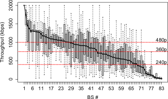
Figure 1: Throughput distribution on base-stations

We observed $158$ unique base-stations, out of which $83$ had $20$ or more samples. Fig. 1 shows the throughput statistics on these $83$ base-stations. All the base-stations, except the last two, were indicated as 3G base-stations; the last two were 2G. While 3G currently claims to provide 2 Mbps in the measured regions, we observed that most base-stations provide much lower throughput during every day mobility scenario. Such achievable throughput cannot cater to the demanding applications, such as video streaming, that mobile users often desire to use during everyday long commutes [4].

For example, around 50% of base-stations that we sampled cannot cater to the recommended bit-rate for a medium sized YouTube stream (320p video), which requires 750 kbps. Recommended bit-rates for YouTube videos of other sizes are shown by the dotted red line in Fig. 1.

We now analyze the variations of throughputs across base-stations on user trajectories. Fig. 2(a) demonstrates the fluctuations in throughputs as the user is traveling on RT-2 on various days. Each row plots one trajectory, with the dots representing the median throughput achieved. The radius of the dot is proportional to the throughput, and the dots are color-coded at 4 thresholds corresponding to different YouTube size videos. Fig. 2(a) shows that mobile users often receive low capacity for extended durations of time. On RT-2, more than 47% of the throughput sampled on the trajectories are below 400 kbps , which is the recommended bit rate for a lower quality (240p) YouTube video.

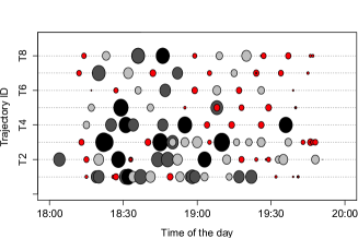
(a) Throughputs on different trajectories in RT-2  

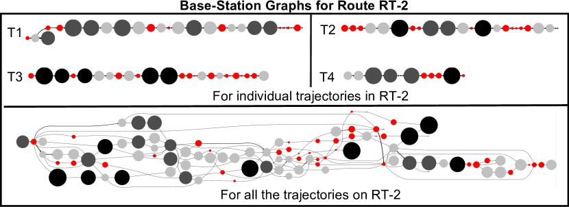
(b) Base-station(BS) graph  

Figure 2: Mobile users constantly experience low throughput on trajectories

We construct a base station graph (BS-graph) for each trajectory, and demonstrate the variance of throughput. Each node in a BS-graph is a base-station. Ideally, a directed edge is drawn between two base-stations if the user hands-off from one to the other. However, due to our limited sampling, an edge denotes that the user was connected to the two base-stations in consecutive samples. The radius of the node is proportional to the median throughput observed when connected to this base-station.

Fig. 2(b) shows the sequence of unique base-stations that the user had recorded on the trajectories. The lower half of Fig 2(b) shows the BS-graph for all trajectories on RT-2, and the upper part of the figure separates the BS-graph for individual trajectories. We use this notion of a chain of base-stations, with the user having some experience on each base-station, to theoretically abstract the mobile user experience on a trajectory. Fig. 2(a) and Fig. 2(b) show that the user has long stretches of time (and sequence base-stations) that degrade user experience.

III Trajectory Utility Maximization Problem

In this section, we design a generic formulation that, given a budget, plans base-station upgrades that maximizes the mobile users’ experience. Our model is practical and useful for today’s cellular operators as it utilizes the already existing data and enables the operator to control key parameters for base-station upgrades. Specifically, we allow the operator to: (1) optimize based on a given budget; (2) define the strictness of when a subscriber’s mobile experience is considered to be poor; (3) utilize active data already stored by many operators, such as call records [8] and deep-packet inspection logs [9], to quantify user experience on a trajectory.

Consider the network $\mathcal{B}$ = {$B_{1}$, …, $B_{n}$} of $n$ base-stations spread across a region. A trajectory $T_{j}$ is represented as a sequence of tuples of the form $\Phi_{i}=\langle B_{i},\Delta_{i},\eta_{i}\rangle$ that captures the user experience. The user on this trajectory was connected to the base-station $B_{i}\in\mathcal{B}$ for a time interval of $\Delta_{i}$ units and received a throughput of $\eta_{i}$ bytes per unit of time. Note that $\eta_{i}$ can be any metric as long as a greater $\eta_{i}$ denotes better experience (e.g., throughput or packet success rate) when associated to a respective base-station. Henceforth, for brevity, we refer to this metric as throughput. As we show in Section V, the trajectories and $\Phi_{i}$’s can be constructed by scanning the active transaction records maintained by the operator.

For ease of notation, we write $B_{i}\in T_{j}$ if the base-station $B_{i}\in\mathcal{B}$ lies on the trajectory $T_{j}$. The length of a trajectory $T_{j}$, denoted by $|T_{j}|$, is simply the count of base-stations that lie on it. Suppose $d$ denotes the maximum length of a trajectory.

For a trajectory $T_{j}$, a base-station $B_{i}\in T_{j}$ is a bottleneck base-station if it offers a degraded quality of service, e.g., an extremely low upload/download speed, a call-drop, etc. In our model, we assume that a base-station $B_{i}$ acts as a bottleneck w.r.t. a trajectory $T_{j}$ if the corresponding throughput is less than a threshold, i.e., $\eta_{i}<\tau$. The value of $\tau$ is computed from a combination of network parameters. A base-station that is a bottleneck for one trajectory may not be a bottleneck for other trajectories since different users may experience different throughputs based on various factors such as data plan, time of the day, etc.

Our goal is to maximally improve the mobile user experience by selectively upgrading $k$ out of $n$ base-stations that act as bottlenecks on some trajectories. Suppose $\mathbf{X}=\{x_{1},\dots,x_{n}\}$ denotes the boolean solution vector such that $x_{i}=1$ if and only if base-station $B_{i}$ is chosen for upgradation and $0$ otherwise.

Our proposed framework allows the network operator to specify any trajectory utility function $W_{j}:(T_{j},\mathbf{X})\rightarrow[0,1]$, defined over each trajectory $T_{j}$ and solution $\mathbf{X}$, that captures the impact of base-station upgrades on the trajectory $T_{j}$. We assume that $W_{j}$ increases as more number of bottleneck base-stations on the trajectory $T_{j}$ get upgraded. In other words, the trajectory utility increases with its quality of experience (QoE). Our aim is to maximize the number of trajectories with high utility.

To do so, given any trajectory utility function $W_{j}$, we map it to a step utility function $U_{j}$ using a threshold $\gamma\ (0\leq\gamma\leq 1)$, henceforth referred to as the bottleneck parameter:

$$U_{j}=\begin{cases}1&\text{ if }W_{j}\geq\gamma\\ 0&\text{ otherwise }\end{cases}$$ (1)

We now formally state the Trajectory Utility Maximization Problem, $\operatorname{TUMP}(\gamma)$.

Problem 1 ($\operatorname{TUMP}(\gamma)$).

Given a base-station network $\mathcal{B}$ of size $n$, a budget parameter $k$, a bottleneck parameter $\gamma$, and a set of $m$ trajectories $\mathcal{T}=\{T_{1},\dots,T_{m}\}$, each of which has an associated utility function $W_{j}$, determine the set of $k$ base-stations to upgrade such that the sum of utilities $\sum_{T_{j}\in\mathcal{T}}U_{j}$ is maximized, where $U_{j}$ is given by Eq. (1).

Intuitively, a solution to a given instance of $\operatorname{TUMP}(\gamma)$ with a high value of $\gamma$ would benefit lesser number of spatially distinct trajectories, as it attempts to utilize the available resources (i.e., upgraded base-stations) to optimize the QoE on these trajectories. On the other hand, a solution to the same instance of $\operatorname{TUMP}(\gamma)$ with a lower value of $\gamma$ would attempt to be more fair in distribution of the available resources across a larger set of spatially distinct trajectories at the cost of allowing limited improvement in QoE. The operator can judiciously tune $\gamma$ based on the budget and desired subscriber experience.

III-A Solution Overview

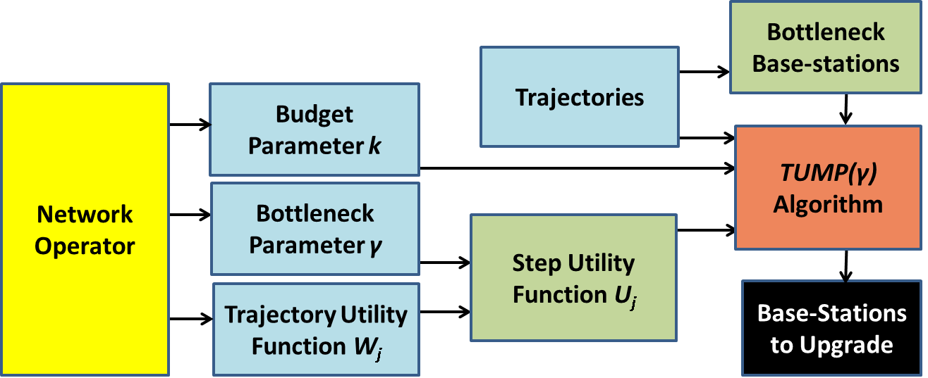
Figure 3: Solution Overview

Fig. 3 outlines the basic steps involved in our solution framework. We construct the user trajectories from call records that the operator has already stored [8, 9]. Given a set of trajectories, we first identify the bottleneck base-stations, based on the throughputs received. A base-station is a candidate for upgrade if it is a bottleneck for any trajectory. The network operator provides a trajectory utility function $W_{j}$ associated with each trajectory $T_{j}$, and the bottleneck parameter $\gamma$. To maximize the number of satisfied trajectories, we map the utility function $W_{j}$ to a step utility function $U_{j}$, using the bottleneck parameter $\gamma$. Finally, we apply any of the proposed algorithms for $\operatorname{TUMP}(\gamma)$ (described in Section IV), and report the $k$ base-stations to be upgraded.

III-B Bottleneck Utility Function

Though the proposed framework allows any trajectory utility function, for the purpose of analysis and evaluation of our approach, this section introduces a special trajectory utility function, namely bottleneck utility function.

Given a trajectory $T_{j}$, we define the weight $w_{ji}$ for each base-station $B_{i}\in T_{j}$, that accounts for the fraction of the total time that the user (on this trajectory) was connected to the base-station $B_{i}$. More precisely, $w_{ji}=\frac{\Delta_{i}}{\sum_{B_{i}\in T_{j}}\Delta_{i}}$. Suppose $b_{ji}$ denotes a bottleneck indicator variable that takes value $1$ if the base-station $B_{i}\in T_{j}$ is a bottleneck base-station w.r.t. the trajectory $T_{j}$, and $0$ otherwise.

Given a trajectory $T_{j}$ and solution $\mathbf{X}$, we define the bottleneck utility function $W_{j}$ as follows:

$$W_{j}=\sum_{B_{i}\in T_{j},b_{ji}=0}w_{ji}+\sum_{B_{i}\in T_{j},b_{ji}=1}w_{ji}.x_{i}$$ (2)

$W_{j}$ essentially captures the fraction of the total time when the user enjoys acceptable QoE on the trajectory $T_{j}$. If all the base-stations on $T_{j}$ are non-bottleneck, then $W_{j}=1$; otherwise, $W_{j}<1$. Henceforth, we consider the bottleneck utility function as the default trajectory utility function.

Based on this, we next define a class of trajectories that enjoy satisfactory QoE after upgradation of the base-stations.

Definition 1 ($\gamma$-bottleneck-free trajectory).

A trajectory $T_{j}\in\mathcal{T}$ is $\gamma$-bottleneck-free if its utility $W_{j}\geq\gamma$ where $W_{j}$ is given by Eq. (2), and $\gamma\in[0,1]$ is the bottleneck parameter.

Of particular analytical interest is the problem instance $\operatorname{TUMP}(\gamma=1)$, denoted henceforth by simply $\operatorname{TUMP}(1)$. In this case, $\forall j=1,\dots,m,\ U_{j}=W_{j}=1$ if and only if all the bottleneck base-stations on the trajectory $T_{j}$ are upgraded. This problem instance is interesting because it is the worst case instance of the $\operatorname{TUMP}(\gamma)$ problem that aims to maximize the number of trajectories that are completely bottleneck-free.

This framework allows the network operator to suitably select the bottleneck parameter $\gamma$ based on the application requirements. For example, $\gamma=1$ is suitable for real-time applications such as voice calls or video conferences whereas $\gamma=0.8$ may suffice for video streaming since video players can mask-off certain durations of low connectivity by buffering. Similarly, even $\gamma=0.5$ may be enough for elastic applications such as background synchronization of emails.

III-C Hardness of $\operatorname{TUMP}(\gamma)$

Next, we show that $\operatorname{TUMP}(\gamma)$ is NP-hard due to a reduction from the $k$-Vertex Cover ($k$-VC) problem [10].

Problem 2 ($k$-VC).

Given an undirected graph $G(V,E)$ where $V$ is the set of $n$ nodes and $E$ is the set of $m$ edges, determine a set $S\subseteq V$ of $k$ nodes that maximizes the number of edges covered by the nodes in $S$, i.e., incident on at least one of the nodes in $S$.

Being a generalization of the vertex cover problem, the $k$-VC problem is NP-hard [10].

Theorem 1.

The $\operatorname{TUMP}(\gamma)$ problem is NP-hard.

Proof.

Given an instance of the $k$-VC problem, $G(V,E)$, we reduce it to an instance of $\operatorname{TUMP}(\gamma)$ as follows. For each node $v_{i}\in V$, we create a base-station $B_{i}\in\mathcal{B}$. For each edge $(v_{i},v_{j})\in E$, we create a trajectory of size $2$, $\{\langle B_{i},\Delta_{0},\eta_{0}\rangle,\langle B_{j},\Delta_{0},\eta_{0}\rangle\}$, where $\Delta_{0}$ and $\eta_{0}$ are arbitrary constant values for time interval and throughput respectively. Also, $\forall T_{j},\forall B_{i}\in T_{j},b_{ji}=1$, i.e., each of the base-stations incident on a trajectory acts as a bottleneck.

If a subset $S\subseteq V$ is a solution to the $k$-VC problem, then the set of base-stations $B_{S}=\{B_{i}|v_{i}\in S\}$ is a solution to the $\operatorname{TUMP}(\gamma)$ problem with $\gamma=0.5$. If the edge $(v_{i},v_{j})\in E$ is covered by the set $S$, then at least one of the two base-stations, $B_{i},B_{j}\in B_{S}$ and, thus, the trajectory $\{\langle B_{i},\Delta_{0},\eta_{0}\rangle,$ $\langle B_{j},\Delta_{0},\eta_{0}\rangle\}$ becomes $0.5$-bottleneck-free, i.e., its utility becomes $1$. Since the subset $S$ maximizes the number of edges covered by it, the solution $B_{S}$ maximizes the number of $0.5$-bottleneck-free trajectories or, in other words, maximizes the sum of trajectory utilities.

Similarly, we argue that if $B$ is a solution to the $\operatorname{TUMP}(\gamma)$ problem with $\gamma=0.5$, then $S_{B}=\{v_{i}|B_{i}\in B\}$ is a solution to the $k$-VC problem. Since $\gamma=0.5$, the utility of a trajectory is maximized if and only if the trajectory becomes $0.5$-bottleneck-free, i.e., at least one of the two base-stations, $B_{i},B_{j}$ on the trajectory, is in the solution $B$. This in turn implies that the edge $(v_{i},v_{j})\in E$ is covered by at least one of the nodes $v_{i},v_{j}\in S$. Since $B$ maximizes the number of $0.5$-bottleneck-free trajectories, the subset $S_{B}$ maximizes the number of edges covered by it.

Since the reduction requires space and time which is polynomial in the size of the input, the proof follows. ∎

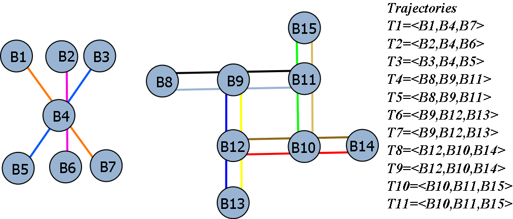
Figure 4: Trajectories in Example 1.

IV Algorithms for $TUMP(\gamma)$

This section describes the algorithms for the $\operatorname{TUMP}(\gamma)$ problem. Firstly, we propose an integer programming based optimal algorithm, namely $IP_{\operatorname{TUMP}(\gamma)}$ and an approximation scheme based on LP relaxation of $IP_{\operatorname{TUMP}(\gamma)}$. Owing to their high running times, both of these algorithms are however, impractical for any reasonably sized dataset. The problem being NP-hard, we next present few approximation algorithms based on greedy paradigm, that not only offer faster running times, but also perform well in practice.

We begin by illustrating a simple example of $\operatorname{TUMP}(\gamma)$ problem, that will be shortly evaluated by different algorithms.

Example 1.

Fig. 4 shows $11$ trajectories, $T_{1},\cdots,T_{11}$, each of length $3$, passing through a set of $15$ base-stations $B_{1},\cdots,B_{15}$. We assume that each base-station is a bottleneck w.r.t. each of the trajectories incident on it. In addition, for ease of analysis, we assume that for a given trajectory, the $\Delta,\eta$ values are same for all the base-stations incident on it. For this reason, we did not list their values in Fig. 4. This assumption eliminates the influence of $w_{ji}$’s on the solution. hus, for any trajectory $T_{j}$ and a base-station $B_{i}\in T_{j}$, $w_{ji}=1/3$. We next observe that while each of the base-stations $B_{9},B_{10},B_{11}$ and $B_{12}$ have a maximum of $4$ incident trajectories, the base-stations $B_{4}$ has $3$ incident trajectories, the base-stations $B_{8}$, $B_{13},B_{14}$ and $B_{15}$ have $2$ incident trajectories and the rest have only $1$ trajectory passing through them. e set $k=3$ base-stations to upgrade as the budget parameter. We evaluate this example for three different values of $\gamma$, as shown in Table II. Following the above assumptions, we find that when $\gamma=0.33$ (resp. $\gamma=0.5$ and $\gamma=1$), it implies that at least one (resp. two and three) of the three base-stations on the trajectory must be upgraded, in order to make it $\gamma$-bottleneck-free. The optimal solutions for each of these cases are shown in the table. ∎

We pose the $\operatorname{TUMP}(\gamma)$ problem in a graph setting. Each instance of the $\operatorname{TUMP}(\gamma)$ problem is associated with a hyper-graph $H=(V,E)$ where $V=\{v_{1},\dots,v_{n}\}$ is the set of $n$ nodes corresponding to the set of base-stations, $\mathcal{B}$, and $E=\{e_{1},\dots,e_{m}\}$ is the set of $m$ hyper-edges corresponding to the set of trajectories, $\mathcal{T}$. A node $v_{i}$ represents a base-station $B_{i}$ and a hyper-edge $e_{j}$ represents the set of base-stations that the trajectory $T_{j}$ passes through, i.e., $e_{j}=\{v_{i}|B_{i}\in T_{j}\}$. The degree of a node is the number of hyper-edges incident on it.

Given a set of nodes $S\subseteq V$, its weight $w(S)$ denotes the number of hyper-edges, $e_{j}$, incident on at least one of the nodes in $S$ such that $T_{j}$ is $\gamma$-bottleneck-free with respect to the nodes in $S$. For $\gamma=1$, $w(S)$ denotes the number of hyper-edges induced on the sub-hyper-graph formed by $S$, i.e., all the nodes of the hyper-edge are contained within $S$.

Referring to this hyper-graph model, henceforth, we shall use the terms node and base-station (and respectively, hyper-edge and trajectory) interchangeably. The example in Fig. 4 shows this hyper-graph setting.

As a pre-processing step to all our algorithms, we discard the trajectories that cannot be made $\gamma$-bottleneck-free by upgrading any set of $k$ base-stations. If the sum of weights of the $k$ bottleneck base-stations with the largest weights is less than $\gamma$, the trajectory can be deemed as infeasible and can be pruned.

IV-A Optimal Algorithm

The optimal solution to the $\operatorname{TUMP}(\gamma)$ problem is represented by the following integer programming formulation, denoted by $IP_{\operatorname{TUMP}(\gamma)}$:

$$\max w_{\gamma} =\sum_{j=1}^{m}U_{j}$$

$$\text{s.t. }\sum_{i=1}^{n}x_{i} \leq k,$$

$$\forall i=1,\dots,n,\ \forall j=1,\dots,m,\quad x_{i},U_{j}\in\{0,1\},$$

and $$\forall j=1,\dots,m,\quad U_{j}\leq\frac{W_{j}}{\gamma}$$

where $W_{j}$ is given by Eq. 2, assuming it to be the bottleneck utility function. The solution $\{\tilde{x},\tilde{U}\}$ of the above IP formulation yields the optimal weight $\hat{w}_{\gamma}$ (i.e., the number of $\gamma$-bottleneck-free trajectories) to the $\operatorname{TUMP}(\gamma)$ problem. Since the utility of each trajectory is at most $1$, necessarily, $\tilde{w}_{\gamma}\leq m$, where $m$ is the total number of trajectories. Since obtaining the optimal solution requires time that is exponential in the input size, it is impractical. Approximation algorithms are, thus, required to solve the problem in practical running times.

IV-B Approximation Algorithms

In the following sections, we present few approximation algorithms for the $\operatorname{TUMP}(\gamma)$ problem.

TABLE II: Utilities derived from different algorithms for Example 1 with $k=3$.

Algorithms	$\gamma=0.33$		$\gamma=0.5$		$\gamma=1$
	Upgrades	Utility	Upgrades	Utility	Upgrades	Utility
Optimal	$B_{4},B_{11},B_{12}$	$11$	$B_{10},B_{11},B_{12}$	$4$	$B_{10},B_{12},B_{14}$	$2$
SIMPLE-GREEDY	$B_{10},B_{11},B_{12}$	$8$	$B_{10},B_{11},B_{12}$	$4$	$B_{10},B_{11},B_{12}$	$0$
INC-GREEDY	$B_{4},B_{11},B_{12}$	$11$	$B_{10},B_{11},B_{12}$	$4$	$B_{10},B_{11},B_{12}$	$0$
DEC-GREEDY	$B_{4},B_{11},B_{12}$	$11$	$B_{10},B_{11},B_{12}$	$4$	$B_{10},B_{12},B_{14}$	$2$

Let $A$ be any approximation algorithm for $\operatorname{TUMP}(\gamma)$ that always returns a feasible solution $S$ with weight $w(S)\geq r.w(OPT)$, for some fixed $r\in[0,1]$, where $OPT$ refers to an optimal solution . Then $r$ is said to be the approximation bound of the algorithm $A$. Moreover, if an algorithm has an approximation bound of $r$ for the $\operatorname{TUMP}(1)$ problem, then $r$ acts as an approximation bound for any $\operatorname{TUMP}(\gamma<1)$ as well, because $\operatorname{TUMP}(1)$ is the worst case instance of $\operatorname{TUMP}(\gamma)$.

IV-C LP

Here, we propose a linear programming (LP) based heuristic for the $\operatorname{TUMP}(\gamma)$ problem. The LP solution is based on the LP relaxation of the integer programming formulation $IP_{\operatorname{TUMP}(\gamma)}$ specified for the optimal solution. This relaxation allows the variables $x_{i},U_{j}$ to take fractional values, i.e., $\forall i,\ \forall j,\ 0\leq x_{i},U_{j}\leq 1$. Assume that $S^{*}=\{x_{i}^{*},U_{j}^{*}\}$ denotes the (optimal) solution to the above linear program. We derive an integer approximate solution $\hat{S}=\{\hat{x_{i}},\hat{U_{j}}\}$ from $S^{*}$ as follows. We pick the highest $k$ values from $(x_{1}^{*},\dots,x_{n}^{*})$ and set the corresponding $\hat{x_{i}}$ to $1$.

The expensive step of this approach is solving the linear program that involves $O(m+n)$ constraints and $O(m+n)$ variables. The running time of this approach, is although considerably less than the optimal algorithm based on integer programming ($IP_{\operatorname{TUMP}(\gamma)}$), but still impractical for any reasonably sized dataset, as shown in the experiments, discussed in Section VI. Therefore, we next, propose a set of approximation algorithms based on greedy paradigm, that not only offer faster running times, but also perform well in practice.

IV-D SIMPLE-GREEDY

For each base-station $B_{i}\in\mathcal{B}$, we define its bottleneck-weight, $\omega_{i}=\{\sum_{j=1}^{m}w_{ji}|b_{ji}=1\}$. Typically, a base-station that acts as a bottleneck for a large number of trajectories for a considerable fraction of their total time will have a high bottleneck-weight, and is thus, a good candidate for upgradation. The simple greedy approach picks the $k$ base-stations having the largest bottleneck-weights.

Example 2.

Consider Example 1. Since each of the base-stations $B_{9},\dots,B_{12}$ have maximal bottleneck-weight $4/3$, this approach will select the base-stations $B_{10},B_{11}$ and $B_{12}$ (breaking ties on higher index of base-station), irrespective of the value of $\gamma$. The utilities, thus obtained for different values of $\gamma$, are listed in Table II. ∎

The primary drawback of this approach is that it is independent of the notion of trajectory utilities. This is why it does not perform well, especially when $\gamma$ is high. Nevertheless, owing to its simplicity, we consider it as the baseline algorithm for $\operatorname{TUMP}(\gamma)$, and compare the performance of other algorithms against it, as discussed in detail in Section VI.

Analysis of SIMPLE-GREEDY

First, we analyze the time and space complexity of SIMPLE-GREEDY, and then analyze its approximation bound.

Theorem 2.

The time and space complexity bounds for SIMPLE-GREEDY are $O(md+n\log k)$ and $O(md)$ respectively, where $m$ is the total number of trajectories, $d$ is the maximum length of any trajectory, $n$ is the total number of base-stations, and $k$ is the budget parameter.

Proof.

First we analyze the time complexity. Given that there are $m$ trajectories, and each of them has length at most $d$, scanning the input and computing the bottleneck-weight of each base-station, takes $O(md)$ time. Further, computation of top-$k$ base-stations w.r.t. their bottleneck-weights takes $O(n\log k)$ time [11] where $n$ is the total number of base-stations and $k$ is the number of base-stations to be upgraded. Thus, the time complexity of SIMPLE-GREEDY is $O(md+n\log k)$.

As we analyze the space complexity, assuming each trajectory is stored as a list of tuples $\Phi$ taking $O(d)$ space, the total input takes $O(md)$ space. We require $O(n)$ space for computation of the bottleneck-weights ( $O(1)$ space for each node). Since $md\geq n$, the space complexity, is thus $O(md)$. ∎

Unfortunately, this algorithm has no approximation bound for the $\operatorname{TUMP}(\gamma)$ problem, as shown in Table IV.

Theorem 3.

SIMPLE-GREEDY has no bounded approximation for $\operatorname{TUMP}(\gamma)$.

Proof.

To show that SIMPLE-GREEDY does not offer any approximation bound, we consider the following instance of $\operatorname{TUMP}(\gamma)$ problem. Let $\mathcal{B}=\{B_{1},\dots,B_{n}\}$ be the set of base-stations, and $\mathcal{T}=\{T_{1},\dots,T_{m}\}$ be the set of trajectories such that $m=\lfloor\frac{n}{2}\rfloor+1$. For $j=1,\dots,m-1$, the trajectory $T_{j}$ of length $2$, passes through the base-stations $B_{j}$ and $B_{j^{\prime}}$ where $j^{\prime}=j+\lfloor\frac{n}{2}\rfloor$. The trajectory $T_{m}$ of length $\lfloor\frac{n}{2}\rfloor$, passes through the base-stations $B_{1},\dots,B_{\lfloor\frac{n}{2}\rfloor}$. We assume that each base-station is a bottleneck for each of the trajectories passing through it. Additionally, for any trajectory, we assume that the $\triangle,\eta$ values are same across all the base-stations that the trajectory passes through. Therefore, we note that for any trajectory $T_{j}$, $j=1,\dots,m-1$, that passes through the base-stations $B_{j}$ and $B_{j^{\prime}}$, $w_{jj}=w_{jj^{\prime}}=0.5$. For trajectory $T_{m}$, for $i=1,\dots,\lfloor\frac{n}{2}\rfloor$, we note that $w_{mi}=1/\lfloor\frac{n}{2}\rfloor$. Therefore the bottleneck weight $\omega_{i}$ for base-station $B_{i}$ is given by:

$$\omega_{i}=\begin{cases}0.5+1/\lfloor\frac{n}{2}\rfloor&\text{ for }i=1,\dots,\lfloor\frac{n}{2}\rfloor\\ 0.5&\text{ for }i=\lfloor\frac{n}{2}\rfloor+1,\dots,n\end{cases}$$ (3)

Thus, for any $2\leq k\leq\lfloor\frac{n}{2}\rfloor$, SIMPLE-GREEDY would select any $k$ base-stations from the set $B_{1},\dots,B_{\lfloor\frac{n}{2}\rfloor}$, due to their higher bottleneck weight. But any such selection cannot make any trajectory $\gamma$-bottleneck-free for $\gamma=1$. On the other hand, an optimal solution would make at least one trajectory $\gamma$-bottleneck-free. Thus, we show that SIMPLE-GREEDY has no approximation bound for $\operatorname{TUMP}(\gamma)$. ∎

The time and space complexity bounds of the proposed algorithms are stated in Table IV. The proofs are provided in [12]. Further, we show that this algorithm has no approximation bound for the $\operatorname{TUMP}(\gamma)$ problem, [12].

IV-E INC-GREEDY

Based on the principle of maximizing marginal gain, this approach starts with an empty set of nodes $S_{0}=\varnothing$, and incrementally adds nodes such that each successive addition of a node produces the maximal marginal gain in the weight of the solution. The algorithm proceeds in iterations $\theta=\{1,\dots,k\}$. In the beginning of iteration $\theta$, suppose the existing solution is the set of nodes $S_{\theta-1}$ with weight $w(S_{\theta-1})$. The node $v_{\theta}$ from the remaining set $V\setminus S_{\theta-1}$ is added such that $w(S_{\theta-1}\cup\{v_{\theta}\})$ is maximal. The new set is referred to as $S_{\theta}$.

In any iteration, if multiple candidate nodes have the same maximal marginal utility, we select the one with the largest bottleneck-weight. Still, if ties remain, then without loss of generality, we break the tie by selecting the node with the highest index (the indices are arbitrary but unique).

Example 3.

We first evaluate INC-GREEDY on Example 1 for $\gamma=0.33$. At iteration $1$, nodes $B_{9},\dots,B_{12}$ have the same maximal marginal utility of $4$ and the same bottleneck-weight $4/3$. So, we pick $B_{12}$ as it has the highest index. Next, we select $B_{11}$, as it offers the maximal marginal utility of $4$. The base-station $B_{10}$ does not offer the maximal marginal gain any more. The base-station $B_{4}$ with marginal gain of $3$ becomes the best choice next. Thus, we obtain a net utility of $11$, which equals the optimal utility.

The selections and utilities for other values of $\gamma$ case, are shown in Table II. Noticeably, for $\gamma=1$, this algorithms offers $0$ utility. Evaluating this case, in iteration $1$, we find that all the base-stations offer $0$ marginal utility, and so we sample the base-stations $B_{9},\dots,B_{12}$ on the basis of maximal bottleneck-weight. Eventually, we pick $B_{12}$ owing to its highest index. In the following $2$ iterations, once again, we find that the marginal utility offered by any base-station is $0$. Respecting the tie-breaking criteria, we pick $B_{11}$ and $B_{10}$ in respective order. This strategy, however, does not make any trajectory $\gamma$-bottleneck-free, and yields $0$ utility. ∎

The next algorithm (DEC-GREEDY) addresses this limitation.

Analysis of INC-GREEDY

Fist we analyze the complexity bounds, followed by the approximation bound.

Theorem 4.

The time and space complexity bounds for INC-GREEDY are $O(md^{2})$ and $O(md)$ respectively.

Proof.

We first analyze the time complexity of the algorithm. As a pre-processing step, the algorithm computes the bottleneck-weight and initial marginal utility for each node, and computes the initial trajectory utility $W_{j}$ for each trajectory. This step takes $O(md)$ time. Next, in any iteration $\theta$, we select the node $v_{\theta}$ that has maximal marginal utility (applying the tie-breaking rules, if necessary), and add it to the set $S_{\theta}$. This step takes $O(n)$ time. Then for each trajectory $T_{j}$ incident on $v_{\theta}$, for each $v_{i}\in V\setminus S_{\theta}$ such that $B_{i}\in T_{j}$, and $b_{ji}=1$, we check if adding $v_{i}$ to $S_{\theta}$ would make $T_{j}$ $\gamma$-bottleneck-free. If so, we increment the current marginal utility of $v_{i}$ by $1$. If $\delta_{\theta}$ is the degree of the node $v_{\theta}$, then this step takes $O(\delta_{\theta}d)$ time. Since $\sum_{i=1}^{n}\delta_{i}\leq md$, hence the total time spent in the above step over $k$ iterations, is $O(md^{2})$. The total time complexity of the algorithm, running over $k$ iterations, is thus $O(md^{2}+kn)$.

To analyze the space complexity, we find that besides the input that takes $O(md)$ space, the algorithm requires $O(1)$ space for each of the trajectories to store their current utilities that gets updated after each iteration. Further, we need $O(1)$ space for each of the nodes to store their marginal utility, bottleneck-weight, and to hold the information if they are selected. Thus, the space complexity of the algorithm is $O(md+m+n)=O(md)$. ∎

The time complexity of this algorithm can be further improved to $O(md^{2}+k\log n)$ by using advanced data structures such as Fibonacci Heaps [13] to store the marginal utilities of the nodes. However since the total time for updating of marginal utilities of the nodes $(O(md^{2}))$ dominates the time for computing the node with maximal marginal gain ($O(k\log n)$), we avoided this implementation.

Unfortunately, similar to SIMPLE-GREEDY, INC-GREEDY has no approximation bound for $\operatorname{TUMP}(\gamma)$.

Theorem 5.

INC-GREEDY has no bounded approximation for $\operatorname{TUMP}(\gamma)$.

Proof.

To show that INC-GREEDY does not offer any approximation bound, we consider the following instance of $\operatorname{TUMP}(\gamma)$ problem. Let $\mathcal{B}=\{B_{1},\dots,B_{n}\}$ be the set of base-stations, and $\mathcal{T}=\{T_{1},T_{2}\}$ be the set of trajectories. Without loss of generality, let $n$ be a even number. Let trajectory $T_{1}$ pass through the base-stations with odd index, i.e., $B_{1},B_{3},B_{5},\dots,B_{n-1}$, and let trajectory $T_{2}$ pass through the base-stations with even index, i.e., $B_{2},B_{4},B_{6},\dots,B_{n}$. We assume that each base-station is a bottleneck for each of the trajectories passing through it. Additionally, for any trajectory, we assume that the $\triangle,\eta$ values are same across all the base-stations that the trajectory passes through. Since there is only a single trajectory (of length $n/2$) incident on each base-station, the bottleneck weight $\omega_{i}$, for any base-station $B_{i}\in\mathcal{B}$, is $2/n$. Let $k=n/2$ and $\gamma=1$.

Now let us evaluate INC-GREEDY on this instance. In each iteration, $1,\dots,k$, the marginal utility of each node is $0$. Respecting the tie-breaking criteria, in iteration $1,\dots,k$, we select the nodes $B_{n},B_{n-1},\dots,B_{\lfloor\frac{n}{2}\rfloor+1}$, respectively. However, by this selection, neither of the trajectories could become $\gamma$-bottleneck-free. On the other hand, an optimal solution would select all the $n/2$ base-stations on either of trajectories, $T_{1}$ or $T_{2}$, thus making at least one trajectory $\gamma$-bottleneck-free. Thus, we show that INC-GREEDY has no approximation bound for $\operatorname{TUMP}(\gamma)$. ∎

The time and space complexity bounds of this algorithm are stated in Table IV. The proofs are provided in [12]. Further, we show that this algorithm has no approximation bound for the $\operatorname{TUMP}(\gamma)$ problem, [12].

IV-F DEC-GREEDY

This algorithm operates in the reverse order by minimizing marginal loss. It starts with the full set of nodes $V$ and successively removes nodes in a manner that minimizes the marginal loss in the weight of the resulting set. More precisely, it starts with $S_{0}=V$, and removes one node in each iteration $\theta=\{1,\dots,n-k\}$. At the start of iteration $\theta$, suppose the existing set of nodes is $S_{\theta-1}$ with weight $w(S_{\theta-1})$. From this set, the node $v_{\theta}$ is removed such that $w(S_{\theta-1}\setminus\{v_{\theta}\})$ is maximal. The new set is referred to as $S_{\theta}$.

Moreover, after each iteration, all trajectories that can no longer be made $\gamma$-bottleneck-free are pruned. In any given iteration, if multiple candidate nodes qualify to be deleted, then the one with the smallest bottleneck-weight is chosen. Still, if there are multiple candidates, the tie is broken by removing the node with the lowest index.

Example 4.

We first evaluate DEC-GREEDY on Example 1 for $\gamma=1$. At iteration $1$, any of the base-stations, $B_{1},B_{2},B_{3},B_{5},B_{6}$ and $B_{7}$, have the same minimal marginal loss in utility of $1$. Respecting the tie-breaking criteria, we prune $B_{1}$. Consequently, trajectory $T_{1}$ becomes infeasible and is, thus, pruned. This results in marginal utility of $B_{7}$ to become $0$, as there is no other incident trajectory on $B_{7}$. So, in the next iteration, we prune $B_{7}$. Proceeding in this manner, the order of deletions of the nodes in subsequent iterations is as shown in Table III. At the end of 12 iterations, we are left with the base-stations $B_{10},B_{12}$ and $B_{14}$ which render 2 trajectories, $T_{8}$ and $T_{9}$, $\gamma$-bottleneck-free, which is same as the optimal algorithm.

Table II shows the output of DEC-GREEDY for other values of $\gamma$, along with Table III which shows the order of deletions of nodes in the $n-k=12$ iterations. ∎

TABLE III: Order of node-deletions by DEC-GREEDY for Example 1.

$\gamma$	Order of Nodes deleted during iteration 1 to 12 $\rightarrow$
$0.33$	$B_{1},B_{2},B_{3},B_{5},B_{6},B_{7},B_{8},B_{13},B_{14},B_{15},B_{9},B_{10}$
$0.5$	$B_{1},B_{2},B_{3},B_{8},B_{13},B_{14},B_{15},B_{5},B_{6},B_{4},B_{7},B_{9}$
$1$	$B_{1},B_{7},B_{2},B_{6},B_{3},B_{4},B_{5},B_{8},B_{9},B_{13},B_{11},B_{15}$

Analysis of DEC-GREEDY

The time complexity analysis of DEC-GREEDY is similar to that of INC-GREEDY, with the difference that in this case there are $n-k$ iterations. Thus the time complexity is $O(md^{2}+(n-k)n)$, as shown in Table IV. Since, $k$ is likely to be less that $n/2$, DEC-GREEDY is expected to take more number of iterations, and is therefore, more expensive in terms of time, when compared to INC-GREEDY. The space complexity of DEC-GREEDY is same as in the case of INC-GREEDY, i.e., $O(md)$.

We next analyze the approximation bound of DEC-GREEDY algorithm.

Theorem 6.

The approximation bound of DEC-GREEDY for $\operatorname{TUMP}(\gamma)$ is ${\binom{k}{d}}/{\binom{n}{d}}$.

Proof.

To analyze the worst case scenario, we assume that each base-station is a bottleneck w.r.t. each of the incident trajectories, and further, $\gamma=1$. Assume that $S_{\theta}$ denotes the set of nodes in the sub-hyper-graph resulting at the end of iteration $\theta=\{1,\dots,n-k\}$. Since $\gamma=1$, $w(S_{\theta})$ denotes the number of hyper-edges induced in this sub-hyper-graph, i.e., all its nodes must be in $S_{\theta}$. Following the above assumption, once the node $v_{\theta}$ is removed, all its incident hyper-edges in $S_{\theta-1}$ are removed, because the corresponding trajectories can no longer become $\gamma$-bottleneck-free. Therefore, the node $v_{\theta}$ (selected to be pruned due to its minimal marginal loss) must have the minimal degree in the sub-hyper-graph induced over the nodes in $S_{\theta-1}$. This ensures that the weight of the resulting set $w(S_{\theta})=w(S_{\theta-1}\setminus\{v_{\theta}\})$ is maximal.

Note that the sum of degrees of nodes in $S_{\theta-1}$ is equal to the sum of the lengths of the trajectories induced in the sub-hyper-graph $S_{\theta-1}$ which is at most $w(S_{\theta-1})d$ where $d$ is the maximum length of any trajectory. Since $|S_{\theta-1}|=n-\theta+1$, the average degree of a node in $S_{\theta-1}$ is at most $\frac{w(S_{\theta-1})d}{|S_{\theta-1}|}=\frac{w(S_{\theta-1})d}{n-\theta+1}$. After DEC-GREEDY removes the node $v_{\theta}$ with minimal degree (which is at most the average degree), the weight of the sub-hyper-graph $S_{\theta}$ is bounded as

$$w\left(S_{\theta}\right) \geq w\left(S_{\theta-1}\right)-w\left(S_{\theta-1}\right)\frac{d}{n-\theta+1}$$

Hence, after $n-k$ iterations

$$w\left(S_{n-k}\right) \geq w(S_{0})\prod_{\theta=1}^{n-k}\left(1-\frac{d}{n-\theta+1}\right)$$

For $\operatorname{TUMP}(1)$, we can assume that $k\geq d$ since any trajectory with $|T_{j}|>k$ can be pruned as it can never be made $\gamma$-bottleneck-free. Hence, using $n\geq k\geq d$ and $w(S_{0})=m$,

$$w\left(S_{n-k}\right) \geq m\frac{k(k-1)\dots(k-d+1)}{n(n-1)\dots(n-d+1)}=m\left(\frac{\binom{k}{d}}{\binom{n}{d}}\right)$$

Since weight of any optimal solution is at most $m$, the approximation bound of DEC-GREEDY is ${\binom{k}{d}}/{\binom{n}{d}}$. ∎

IV-G Equivalence of Incremental and One Shot Upgrades

An interesting and very useful property of the proposed INC-GREEDY and DEC-GREEDY algorithms is that they naturally support incremental upgrades of base-stations. Note that INC-GREEDY (respectively, DEC-GREEDY) selects (respectively, prunes) one base-station in each iteration, and the selection criteria is independent of the budget parameter $k$. Hence, it can be shown that, for both these algorithms, piecewise incremental upgrades is equivalent to a one-shot upgrade, provided the total budget is same in both the cases.

More formally, if $k_{1}+k_{2}+\dots=k\ (\forall k_{i}>0)$, then successive applications of INC-GREEDY (respectively DEC-GREEDY) with budget parameters $k_{1}$, followed by $k_{2}$, etc., would upgrade the same set of base-stations as a one-shot application of INC-GREEDY (respectively, DEC-GREEDY) would with budget parameter $k$. This property is very important as it allows the network planners to upgrade as and when some budget is allocated. The overall effect on the network is the same even if the entire budget was made available at one go. First we establish this claim for INC-GREEDY, followed by DEC-GREEDY.

Proposition 1.

Given any instance of $\operatorname{TUMP}(\gamma)$,

$$S_{k}=S_{\theta}\cup S^{\prime}_{k-\theta},\ \forall 1\leq k\leq n,\,1\leq\theta\leq k$$ (4)

where $S_{k}$ is the set of nodes (corresponding to the upgraded base-stations) by INC-GREEDY ($k$), and $S_{\theta}$, $S^{\prime}_{k-\theta}$ are the sets of nodes provided by two consecutive operations of INC-GREEDY ($\theta$) on $V$, and INC-GREEDY ($k-\theta$) on $V\setminus S_{\theta}$ respectively.

Proof.

Observe that the algorithm always selects the nodes in $V$ in a consistent order. This follows from the fact that the algorithm breaks all ties deterministically (if needed, using the index of the nodes). Therefore, without loss of generality, assume that INC-GREEDY ($n$) applied on the node set $V$ selects the nodes in the order $v_{1},\dots,v_{n}$. Hence, INC-GREEDY ($k$) applied on the node set $V$ would select the nodes $S_{k}=\{v_{1},\dots,v_{k}\}$. For $\theta\leq k$, $S_{\theta}=\{v_{1},\dots,v_{\theta}\}\subseteq S_{k}$. Applying INC-GREEDY ($k-\theta$) on the set $V\setminus S_{\theta}=\{v_{\theta+1},\dots,v_{n}\}$ would select the nodes $S^{\prime}_{k-\theta}=\{v_{\theta+1},\dots,v_{k}\}$. Hence, $S_{k}=S_{\theta}\cup S^{\prime}_{k-\theta}$. ∎

Proposition 2.

Given any instance of $\operatorname{TUMP}(\gamma)$,

$$S_{n-k}=S_{n-\theta}\cup S^{\prime}_{n-k},\ \forall 1\leq k\leq n,\,1\leq\theta\leq k$$ (5)

where $S_{n-k}$ is the set of nodes retained (corresponding to the upgraded base-stations) by applying DEC-GREEDY ($k$) on $V$, and $S_{n-\theta}$, $S^{\prime}_{n-k}$ are the sets of nodes retained by two consecutive operations of DEC-GREEDY ($\theta$) on $V$, and DEC-GREEDY ($k-\theta$) on $V\setminus S_{n-\theta}$ respectively.

Proof.

Observe that the algorithm always prunes the nodes in $V$ in a consistent order. This follows from the fact that the algorithm breaks all ties between the nodes deterministically (if needed, using the index of nodes). Therefore, without loss of generality, assume that DEC-GREEDY ($0$) applied on the node set $V$ prunes the nodes in the order $v_{1},\dots,v_{n}$. Hence, applying DEC-GREEDY ($k$) on $V$ would prune the nodes $v_{1},v_{2},\dots,v_{n-k}$ and return $S_{n-k}=\{v_{n-k+1},\dots,v_{n}\}$. For $\theta\leq k$, $S_{n-\theta}=\{v_{n-\theta+1},$ $\dots,v_{n}\}\subseteq S_{n-k}$. Applying DEC-GREEDY ($k-\theta$) on the set $V\setminus S_{n-\theta}=\{v_{1},\dots,v_{n-\theta}\}$ would prune the nodes $v_{1},\dots,v_{n-k}$ and return $S^{\prime}_{n-k}=\{v_{n-k+1},\dots,v_{n-\theta}\}$. Hence, $S_{n-k}=S_{n-\theta}\cup S^{\prime}_{n-k}$. ∎

Summary of the Algorithms

A summary of analysis of the proposed greedy algorithms is presented in Table IV. While SIMPLE-GREEDY, and INC-GREEDY have lower time complexities than DEC-GREEDY, but they do not offer any bounded approximation. DEC-GREEDY, on the other hand, offers a bounded approximation with the trade-off of higher running time.

TABLE IV: Summary of Analysis of Algorithms for $\operatorname{TUMP}(\gamma)$

Algorithms	Time Complexity	Space Complexity	Approx. Bound
SIMPLE-GREEDY	$O(md+n\log k)$	$O(md)$	0
INC-GREEDY	$O(md^{2}+kn)$	$O(md)$	0
DEC-GREEDY	$O(md^{2}+(n-k)n)$	$O(md)$	${\binom{k}{d}}/{\binom{n}{d}}$

V Evaluation Methodology

We show the efficacy of the algorithms using real as well as synthetic but realistic datasets. Our formulation considers two critical parameters whose values are best decided by the operator: the budget ($k$), and the threshold $\gamma$ (which signifies the desired satisfaction level on the trajectory that the operator is targeting). The input trajectories are generally chosen by the cellular operator based on the target subset of subscribers (e.g., based on focused micro-segments such as long-commuting 3G subscribers). The trajectories of subscribers are readily available to operators in Call Detail Records (CDRs) and deep-packet inspection logs [8].

V-A City and Network Generator (CING)

Real data about trajectories of subscribers is generally not publicly available. Hence, we designed City and Network Generator (CING) tool to generate representative traces of population distribution, mobility and network topology. We evaluate our protocols under such synthetic data and, also, on one real trace data set [14]; we describe these data sets later. CING models both the city population and network deployment by considering: (1) how users travel in a city, and (2) how base-stations (BS) are deployed. We now briefly explain these aspects.

City Model:

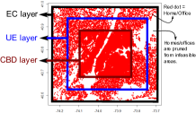
Figure 5: CING City Model: Example of a virtual NYC

We model a virtual city based on the existing map-data and the observed spatial distribution of homes and offices. We employ a concentric city model, where the city is divided into a few layers [15]. The Central Business District (CBD) constitutes the city-center, and usually has high office density. The Urban Envelopes (UE) are around the CBD. Edge Cities (EC) surrounds the main city’s UE.

CING reads parameters such as dimensions and office/residential densities in various layers of the city, and creates synthetic user homes and offices. Lang et. al. have reported these information for thirteen popular US cities [15]. However, only some regions of the city has been surveyed. Since we are interested in movement of subscribers in a city, directly using the partial city information leads to biased trajectories. Hence, we extrapolate the parameters reported to the entire city dimension. City dimension is computed by latitude and longitude information the outer-most layer of the city that is surveyed (the EC layer). We then construct concentic rectangles of CBD, SD, UE and EC layers for each city as shown in Fig. 5.

The areas of the layers are scaled proportionally to match the overall area. We distribute homes/offices in each layer according to the observed spatial densities [15]. Using map data, we then prune the locations that are in inaccessible regions, such as locations within the rivers (see Fig. 5).

Currently, we associate home and office as User hangouts. A user hangout is represented by a spatial location and most frequent user’s arrival and departure times. We artificially populate the home and office hangouts by observing weekday commute patterns of the users.; for example, by observing that the user leaves home at a random time from 7 AM to 11 PM to commute to office. If the spatio-temporal hangout information is available (e.g., as a result of mining real profile data, social network data or CDR data), the data can hence also be provided as an input to CING tool rather than generating virtual locations. Network Model: CING generates base-stations (BS) such that the number of BS in a region is proportional to the number of homes and offices. Our network consists of 82% 2G BS, based on the deployment statistics of a major Indian cellular operator [5]. We mark 20% of the BS as congested. Based on our measurement observations (Section II), we randomly choose per-user throughput within $[20,80]$, $[50,150]$, $[20,400]$ and $[300,2000]$ kbps for congested 2G, non-congested 2G, congested 3G and non-congested 3G BS respectively.

Trajectory Model:

The trajectory properties such as the path taken from origin to destination affects the user’s experience. CING derives the road-network graph from the OSM map-data [16]. It computes the trajectories of the user by simulating user movement on road between home to office (using the shortest path algorithm). For each road trajectory thus computed, we compute the sequence of base-stations by assuming a hand-off policy where a user is connected to the nearest base-station at any location. The time connected to a base-station based on the road-speeds and BS coverage. The throughput of the user is dependent upon the per-user throughput of the BS and the duration of association.

V-B Data sets

We evaluate the performance of the proposed algorithms using both real and synthetic data.

a) Data set from real traces: The Reality Mining (RM) data set lists the base-station handoffs of more than $100$ users [14]. Most of the users belong to MIT and, hence, the set is biased.

We use this data set to study optimizing trajectories of targeted subscribers with similar spatial hangouts and interests. We extract the sequence of base-station IDs that a user connects. We break the sequence of base-stations into trajectories where the user might have moved; we break a trajectory when there is no change in base-station for more than $30$ minutes. We prune the data to include mobile trajectories of users which have more than 10 base-stations. We also remove trajectories with sequence of base-stations showing a ping-pong handoff pattern [17]. The data set has 3819 trajectories and 17975 base-stations.

We first extract the trajectories by assuming that the a trajectory starts if the user is previously static for more than 30 minutes. The data also contains noisy trajectories, primariy because of: (1) base-station IDs which are out of the city are recorded, and (2) handoffs that often cause ping-pong effect where the device swaps between a set of base-stations even when the user is not moving [17]. Such outlier base-stations and trajectories are pruned; we remove 1000 base-stations that have the least number of trajectories passing through them, and only consider trajectories that have a length of greater than 10.

We finally get $3819$ trajectories and $17975$ base-stations. Note that there is no base-station location information in this data; however, ID suffices for our evaluation.

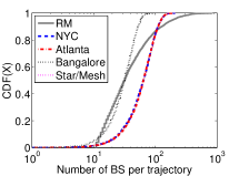
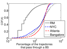
Figure 6: Distribution of trajectory length and degree of a base-station: The degree of the base-station is normalized to the number of trajectories present in the scenario.

RM has 3,819 trajectories and 17,975 base-stations. Fig. 6 shows the CDF of the trajectory length and the degree of a base-station (normalized to the percentage of trajectories that pass through a base-station). The data shows a highly skewed distribution, with many base-stations having very low degree (when compared to the city movement in pure synthetic city data). We conjecture that this is due to the biased set of users; many trajectories often visit a very few base-stations near MIT.

TABLE V: Synthetic data sets: We also evaluate Mesh topology and real traces from Reality Mining (RM) data set.

Star	Bangalore		Atlanta		New York (NYC)
Home and Office	Home	Office	Home	Office	Home	Office
$10\times 14$ $\text{km}^{2}$	$18\times 18$ $\text{km}^{2}$		$42\times 61$ $\text{km}^{2}$		$46\times 64$ $\text{km}^{2}$
$5$k traj; $430$ BS	$25$k traj; $1,894$ BS		$50$k traj; $11213$ BS		$50$k traj; $13860$ BS

b) Synthetic data sets: We generate three classes of datasets, as summarized in Table V.
1. Star and Mesh: These topologies have artificially generated distribution to highlight upgrades in extreme cases of population distribution. Star has a dense CBD with offices, and users commute from their home in a thin UE layer. Mesh indicates a large city where people are equally likely to move in any direction. Here, trajectories are randomly assigned to base-stations with trajectory length distribution similar to Star.
2. New York City (NYC) and Atlanta: We generate two representative large US cities of differing population distributions [15]. NYC has a large CBD with dense offices, while Atlanta’s CBD is small and relatively sparse. Hence, NYC dataset consists of more concentric trajectories, and Atlanta’s trajectories are spread out.
3. Bangalore: We simulate an Indian city, where the population distribution is different than USA. Offices are concentrated in business areas, and homes are spread out across city.

Fig. 6 shows the trajectory length and percent of trajectories incident on base-stations in different data sets. When compared to the RM data set, the synthetic set has higher degree of trajectories incident on each base-station since we consider people moving from all parts of the city towards their respective offices.

VI Results

We measure the effectiveness of the algorithms by computing the percentage of trajectories that are $\gamma$-bottleneck-free, which is an indication of the percentage of mobile users who will be satisfied by the upgrade. We first analyze small-scale regions in the city to understand the effect of model parameters, and then we show the improvements in large-scale city-wide scenarios.

VI-A Comparison with the Optimal

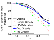
(a) Performance of DEC-GREEDY is close to optimal  

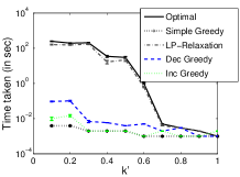
(b) Time comparison: Our algorithms are 3-4 orders faster  

Figure 7: Comparison of different schemes w.r.t. Optimal

We extracted the trajectories in a miniature 2x2 km² area from Bangalore dataset. Since the problem is NP-hard, the optimal solution does not scale up for larger city networks. Therefore, we compared the performance of our algorithms against the optimal solution on this small dataset. This region had 1405 trajectories and 30 base-stations, out of which we chose to optimize 9 base-stations. Since each dataset has different number of base-stations, we analyze the results with the fraction of BS to be upgraded, $k^{\prime}=\frac{k}{n}$. In the above scenario, $k^{\prime}=\frac{9}{30}=0.3$.

We also compare with LP-Relaxation based approach [18], which was discussed in Section IV. Fig. 7(a) compares the performance of the algorithms at different $\gamma$’s, and Fig. 7(b) shows the run-time for $\gamma=1$. Our algorithms, especially DEC-GREEDY, provide similar performances as optimal and LP-Relaxation, while running 3-4 orders of magnitude faster. SIMPLE-GREEDY fails to provide good user experience at higher $\gamma$.

INC-GREEDY is also closer to optimal; however the selfish choices of the algorithm during initial iterations results in a lower performance. We explain the reasons in more detail later.

VI-B Effect of budget allocation, QoS and trajectory lengths

We choose a 5x5 km² area in Bangalore to demonstrate the detailed effects of basic parameters; a larger scale city analysis is later discussed in Section VI-C. This area has 23,000 trajectories with 107 BS. There are 4240, 5420, 8470 and 5430 trajectories with lengths between $[1,5]$,$[6,10]$, $[11,15]$ and $[16,20]$, respectively.

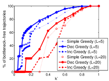
(a) Varying budget (k’); $\gamma=1$.  

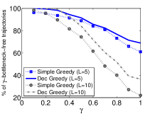
(b) Relaxing QoS ($\gamma$); $k^{\prime}=0.2$  

Figure 8: Effect of trajectory length (L), $k^{\prime}$ and $\gamma$: Our algorithms are well-suited for network upgrades when stricter QoS has to be delivered over longer trajectories with low budgets

1. Effect of budget allocation: Operators incrementally allocate small budgets for upgrades. For example, $k^{\prime}\leq 0.2$ is a representative annual budget of a major Telco [5]. Fig. 8(a) shows the effect of altering the budget ($k^{\prime}$) when the operator chooses to ensure strict QoS to the mobile user ($\gamma=1$). DEC-GREEDY consistently outperforms SIMPLE-GREEDY across different budgets. Note that DEC-GREEDY can be repeatedly applied in increments as more budget becomes available. Hence, the operator can consistently provide better performance than SIMPLE-GREEDY as the network evolves.

INC-GREEDY yields better results than SIMPLE-GREEDY at low $k^{\prime}$. However, its performance is worse than SIMPLE-GREEDY at intermediate $k^{\prime}$-values. This happens as, at each iteration, INC-GREEDY chooses to upgrade the BS that provides immediate benefits; the benefit lies in converting a bottleneck trajectory to $\gamma$-bottleneck-free. This short-term focus on immediate satisfaction biases INC-GREEDY to miss out on choosing BSes that are beneficial to a larger number of trajectories which could have been possibly identified in later iterations.
2. Effect of trajectory lengths: Fig. 8(a) shows the effect of optimizing experiences along short and long trajectories. If the operator chooses to upgrade short trajectories, SIMPLE-GREEDY approach provides comparable performance as DEC-GREEDY. However, if the long-commuting trajectories are to be optimized, DEC-GREEDY approach provides substantial gains, especially for small budgets.

The INC-GREEDY algorithm starts providing better gains for lower $k^{\prime}$ values than SIMPLE-GREEDY. However, DEC-GREEDY consistently outperforms the other two algorithms across different trajectory lengths.
3. Strictness of QoS: Fig. 8(b) shows the effect of relaxing the strictness of the QoS provided to the mobile user (reducing the value of $\gamma$). For smaller $\gamma$ or for shorter trajectories, SIMPLE-GREEDY scheme is comparable to DEC-GREEDY; there are a few highly visited BS on the trajectory, which are candidates for optimizing in SIMPLE-GREEDY approach, which also renders the trajectory $\gamma$-bottleneck-free. However, when stricter user experience is needed over longer trajectories, DEC-GREEDY provides significant benefits over SIMPLE-GREEDY.

VI-C City-scale evaluation

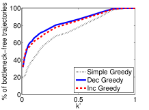
(a) Reality Mining  

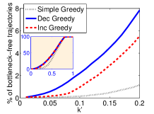
(b) Atlanta  

Figure 9: Performance of TUMP($\gamma=1$) in different scenarios: DEC-GREEDY and INC-GREEDY consistently outperform SIMPLE-GREEDY. With an upgrade budget $k^{\prime}=0.2$, our algorithms perform 3-8 times better in improving the user quality of service on trajectories in different city geographies when compared to greedy location-based base-station upgrades.

Fig. 9 shows the performance of algorithms in different datasets. In the real RM scenario, INC-GREEDY and DEC-GREEDY algorithms consistently provide more than 10-20% improvement when the budget is medium to low. In this biased distribution, few BS (near MIT) are frequently visited by many trajectories. While SIMPLE-GREEDY optimizes frequently accessed BS, it fails to optimize the QoE of frequently accessed trajectories.

In the simulated datasets, DEC-GREEDY and INC-GREEDY constantly outperform SIMPLE-GREEDY. However, the improvement for low $k^{\prime}$ is not as pronounced as in RM dataset since trajectories are spread across the entire city, and hence selecting relevant BS is hard. We also highlight the regions of $k^{\prime}\leq 0.2$ in Fig. 9.

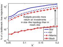
(a) Star-like vs. Mesh-like 

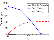
(b) Runtime on Atlanta data-set  

Figure 10: Impact of population and runtime: Star topologies provide more marginal returns for trajectory optimization. The runtime of INC-GREEDY increases as $k^{\prime}$ increases. However, DEC-GREEDY has a reverse trend.

1. Implications of Population Distribution: We observed that NYC consistently provides higher marginal gains than Atlanta. This is because NYC has a high office density in the center, and trajectories form a star-like topology. Upgrading a few BS at the center, hence, benefits a large number of trajectories. In contrast, Atlanta’s trajectories do not form a pronounced star-topology.

Fig. 10(a) compares the performance of DEC-GREEDY in: (1) artificial Star and Mesh topologies, and (2) realistic star-like NYC and mesh-like Atlanta, to highlight the impact of population distribution. Star-like topologies continuously provide significant improvement on small increases in budget. Unlike Star, Mesh requires a large budget ($k$) to provide good performance. For example, for a budget $k=0.2$, Star data-set provides two orders better improvement than Mesh. Hence, while rolling out new upgrades in cities, the operator has to be cognizant that cost of providing better user experience in a star-like city is lower than in a mesh-like city.

2. Runtime comparison: Fig. 10(b) shows the runtime of different algorithms on the Atlanta data-set for $\gamma$=1. DEC-GREEDY and INC-GREEDY are slower than SIMPLE-GREEDY since both these algorithms are iterative. The running time of INC-GREEDY increases as $k$ increases, whereas DEC-GREEDY has a reverse trend.

VII Related Work

To the best of our knowledge, there is no literature that incorporates mobility pattern of the users for base-station upgrades. The related areas can be broadly classified into handoff protocols and radio frequency (RF) planning.
(1) Handoff protocols: These protocols improve connectivity by associating a device with a better base-station [19]. They fail to improve experience if the base-stations are inherently limited in resources (e.g., 2G base-stations).

Other techniques, such as Cell breathing, dynamically alter the coverage area based on the load [20]. While this provides high-capacity to static users, it does not explicitly address the problem of eliminating bottleneck across trajectories.

In contrast to the above protocol based approaches, we focus on the macro-level problem of base-station network planning.
(2) RF planning: RF planning techniques optimize the transmission power, frequency, load and location of the base-station for providing better coverage and/or capacity [6, 21, 22, 23]. RF planning configures base-stations to ensure adequate signal-to-noise ratio (SNR) at the devices, considering the interference from neighboring cells [24, 25]. Some radio planning also considers frequency allocation and cell coverage optimization to cater to mobile users [23]. Most of the RF planning tools, such as Atoll [7], utilize drive tests and carrier wave (CW) measurements to recognize the bottlenecks [6]. Such active measurements inherently limit measuring actual user experiences; they cannot scale to measuring the millions of subscriber trajectories. Other short-range technologies [26, 2, 3] are susceptible to frequent handoffs for mobile users.

In summary, unlike the above studies, we explicitly consider macro-cell planning for providing better user-experience along users’ trajectories. We use user’s call logs, instead of passive measurements, to quantify mobile user experience.

VIII Conclusions

Macro-cell planning for mobile users is a relatively unexplored problem in the evolution of heterogeneous cellular network architectures. This paper addressed the problem of performing macro-cell base-station upgrades by accounting for the mobile user satisfaction along their trajectories.

We conducted a measurement-based experiment to show that mobile users suffer from degraded quality of experience on their everyday commute trajectories. Based on our findings, we formulated a generic problem that plans macro-cell upgrades to optimize mobile user experience. Our formulation utilizes active logs to quantify user experience. In addition, our formulation enables the operators to plan the upgrades in a way that is cognizant of their business needs and constraints. This is done by allowing the operators to define key parameters such as the budget for upgrades, desired satisfaction level on the trajectory, and a micro-segment of the mobile users whose mobile experience has to be optimized (e.g., high-value 4G customers with long commutes).

We proved the NP-hardness of the problem, designed two approximation algorithms, and proved their approximation bounds. We designed a synthetic city and network trace generator, and showed the dependence of planning budget and algorithm effectiveness in various population distributions. Our algorithms consistently enable the operator to achieve 3-8 times better user experience than simple location-based greedy heuristics for the same budget. In future, we plan to address problems in “continuous network planning” systems that ensure quality of experience for mobile users.

References

- [1] Booz&Co, “Avoiding the Slippery Slope: How GCC Telecom Operators Can Improve Profitability?” http://www.strategyand.pwc.com/media/file/Strategyand-GCC-Telecoms-Improve-Profitablity.pdf, Oct 2013.
- [2] “Small cell,” http://en.wikipedia.org/wiki/Small˙cell.
- [3] V. Chandrasekhar, J. Andrews, and A. Gatherer, “Femtocell Networks: A Survey,” in IEEE Comm Magazine, vol. 46, Sept. 2008.
- [4] Wandera, “Enterprise Mobile Data Report - Q3,” http://www.iroam.com/sites/all/themes/elegantica/documents/Enterprise%20Mobile%20Data%20Report%20-%20Q3.pdf, Oct 2013.
- [5] Bharti Airtel Limited, “Quarterly report, March 31, 2014,” online, Apr 2014, available at http://www.airtel.in/wps/wcm/connect/e10e645b-d938-4299-9761-4239f8b543e5/Bharti-Airtel-Limited˙Quarterly-Report˙March-31-2014.pdf?MOD=AJPERES.
- [6] L. Song and J. Shen, Evolved cellular network planning and optimization for UMTS and LTE. CRC Press, 2010.
- [7] Forsk, “Atoll: Wireless Network Engineering Software,” http://www.forsk.com/atoll/.
- [8] 3GPP TS 25.413, “UTRAN Iu interface RANAP signalling,” http://www.3gpp.org/DynaReport/25413.htm.
- [9] Sandvine, “Policy Traffic Switch,” https://www.sandvine.com/platform/policy-traffic-switch.html, July 2014.
- [10] M. Langberg, “Approximation algorithms for maximization problems arising in graph partitioning,” Ph.D. dissertation, Weizmann Institute of Science, 1998.
- [11] D. E. Knuth, Art of Computer Programming, Volume 3: Sorting and Searching (2nd Edition), 2nd ed., 1998.
- [12] “Trajectory aware macro-cell planning for mobile users: Extended paper,” https://dl.dropboxusercontent.com/u/73236979/FullTUMP.pdf.
- [13] M. L. Fredman and R. E. Tarjan, “Fibonacci heaps and their uses in improved network optimization algorithms,” J. ACM, vol. 34, no. 3, pp. 596–615, Jul. 1987. [Online]. Available: http://doi.acm.org/10.1145/28869.28874
- [14] N. Eagle, A. S. Pentland, and D. Lazer, “Inferring friendship network structure by using mobile phone data,” PNAS, vol. 106, no. 36, 2009.
- [15] T. S. Robert E. Lang and J. LeFurgy, “Beyond edge city: Office geography in the new metropolis,” National Center for Real Estate Research, Tech. Rep., Feb 2006.
- [16] “Open street map,” http://www.openstreetmap.org/.
- [17] R. T. Juang, H.-P. Lin, and D.-B. Lin, “An improved location-based handover algorithm for GSM systems,” in Wireless Communications and Networking Conference, 2005 IEEE, vol. 3, 2005, pp. 1371–1376.
- [18] Wikipedia, “Linear programming relaxation,” http://en.wikipedia.org/wiki/Linear˙programming˙relaxation, July 2014.
- [19] A. Sgora and D. Vergados, “Handoff prioritization and decision schemes in wireless cellular networks: a survey,” IEEE Communications Surveys Tutorials, vol. 11, no. 4, pp. 57–77, 2009.
- [20] A. Sang, X. Wang, M. Madihian, and R. D. Gitlin, “Coordinated load balancing, handoff/cell-site selection, and scheduling in multi-cell packet data systems,” in MobiCom ’04, 2004, pp. 302–314.
- [21] C. Peng, S.-B. Lee, S. Lu, H. Luo, and H. Li, “Traffic-driven power saving in operational 3g cellular networks,” in MobiCom ’11. ACM, 2011, pp. 121–132.
- [22] E. Amaldi, A. Capone, and F. Malucelli, “Radio planning and coverage optimization of 3G cellular networks,” Wirel. Netw., vol. 14, no. 4, pp. 435–447, 2008.
- [23] R. Lifjens, “The impact of mobility on UMTS network planning,” in IEEE VTC 2001 Spring, vol. 4, 2001, pp. 2539–2543 vol.4.
- [24] C. Glasser, S. Reith, and H. Vollmer, “The complexity of base station positioning in cellular networks,” Discrete Appl. Math., vol. 148, no. 1, pp. 1–12, Apr. 2005.
- [25] M. Galota, C. Glasser, S. Reith, and H. Vollmer, “A polynomial-time approximation scheme for base station positioning in umts networks,” in DIALM Workshop, 2001, pp. 52–59.
- [26] N. Banerjee, M. D. Corner, D. Towsley, and B. N. Levine, “Relays, base stations, and meshes: Enhancing mobile networks with infrastructure,” in MobiCom ’08. ACM, 2008, pp. 81–91.