I Introduction

The Internet of Things (IoT) is expected to foster the development of 5G wireless networks and requires efficient access of sporadic traffic generating devices. Such devices are most of the time inactive but regularly access the Internet for minor/incremental updates with no human interaction, e.g., machine-type-communication (MTC). Sporadic traffic will dramatically increase in the 5G market and, obviously, such traffic should not be forced to be integrated into the bulky synchronization procedure of current 4G cellular systems [2, 3].

The new conceptional approach in this paper is to use an extended physical layer random access channel (PRACH), which achieves device acquisition and (possibly small) payload transmission ”in one shot”. Similar to the implementation in UMTS, the goal is to transmit small user data packets using the PRACH, without maintaining a continuous connection. So far, this is not possible in LTE, where data is only carried using the physical uplink shared channel (PUSCH) so that the resulting control signaling effort renders scalable sporadic traffic (e.g., several hundred nodes in the cell) infeasible. By contrast, in our design a data section is introduced between synchronous PUSCH and standard PRACH, called D-PRACH (Data PRACH) supporting asynchronous data transmission [1]. Clearly, by doing so, sporadic traffic is removed from standard uplink data pipes resulting in drastically reduced signaling overhead and complexity. In addition, this would improve operational capabilities and network performance as well as user experience and life time of autonomous MTC nodes [2, 3]. Waveform design in this context is a very timely and important topic [4, 5, 1]. Of particular importance is also the line of work in the EU projects METIS (www.metis2020.eu) and 5GNOW (www.5gnow.eu).

We assume that each D-PRACH’s data resource contains only a very few number of subcarriers (about 5-20 subcarriers). In addition, in a 5G system, we can expect that there is a massive number of MTC devices, which will concurrently employ these data resources in an uncoordinated fashion. In the simplest approach, the D-PRACH uses the guard bands between PRACH and PUSCH, which is the focus of this paper. We show that waveform design in such a setting is necessary since the OFDM waveform used in LTE cannot handle the highly asynchronous access of different devices with possible negative delays or delays beyond the cyclic prefix (CP). Clearly, guards could be introduced between the individual (small) data sections and to the PUSCH which, though, makes the approach again very inefficient. Our results indeed show that up to four subcarriers can be obtained compared to a standard 4G OFDM setting.

For waveform design, we propose a bi-orthogonal frequency division multiplexing (BFDM) based approach where we replace orthogonality of the set of transmit and receive pulses with bi-orthogonality, i.e., they are pairwise (not individually) orthogonal. Thus, there is more flexibility in designing the transmit prototype pulse (or waveform), e.g., in terms of side-lobe suppression and robustness to time and frequency asynchronisms [8]. The BFDM approach together with a suitable waveform is well suited to sporadic traffic, since the PRACH symbols are relatively long so that transmission is very robust to (even negative) time offsets. In addition, BFDM is also more robust to frequency offsets in the transmission, which, as well-known, typically sets a limit to the symbol duration in OFDM transmission. Finally, the concatenation of BFDM and OFDM symbols together in a frame requires a good tail behavior of the transmit pulse in order to keep the distortion to the payload carrying subcarriers in PUSCH small. The excellent and controllable tradeoff between performance degradation due to time and frequency offsets is the main advantage of BFDM with respect to conventional OFDM.

We investigate the performance of the proposed approach using mathematical analysis and numerical experiments where, for comparison, a standard LTE system serves as a baseline. A part of the numerical results were already presented in [1]. We show how the new approach can actually reduce the interference to the PUSCH region, experienced in particular by users whose resources are close to the PRACH. Moreover, we demonstrate that the performance in the new D-PRACH region is significantly improved by the pulse-shaping approach when multiple, completely asynchronous, users transmit data in adjacent frequency bands.

I-A System model

We consider a simple uplink model of a single cell network, where each mobile station and the base station are equipped with a single antenna. We assume there exist two channels –in LTE terminology– the PUSCH and the PRACH. In the PUSCH, the data bearing signals are transmitted from synchronized users to the base station using SC-FDMA. A small part of the resources is reserved for PRACH, in which, at the first step of the RACH procedure, users send preambles that contain unique signatures. In this paper, we mainly deal with the PRACH design, trying to leave PUSCH operations as unaffected as possible. Specific system parameters can be found in Table I and standard textbooks [9].

The time-frequency resource grid for the described channels is illustrated in Figure 1. To minimize the interference between the channels, several subcarriers on both sides of the PRACH are usually unused and serve as a guard band to PUSCH. In this paper, however, the D-PRACH is located here, i.e., some users represented by specific signatures use this region to send data by sharing the small number of available subcarriers. Naturally, these users may be completely asynchronous to either PUSCH or to each other, which is a serious challenge for OFDM and will be handled by the BFDM approach using the so-called ”spline” waveform, which has ”good” localization properties in time and frequency.

Figure 1: PRACH (blue) and PUSCH (red) regions. A guard interval (GI) separates PUSCH from PRACH in LTE (gray). Parts of this area are used for data transmissions of asynchronous users (indicated in green) in a novel D-PRACH, whose size can be variably determined by MAC. Rows in this illustration do not represent true subcarrier quantities.

Remark 1.

An important property of the system is that each user can use some autonomous timing advance (ATA), introduced in [10], with respect to the LTE broadcast signal. This will lead to possibly negative as well as positive time delays of each user with respect to the receiver’s ”reception” window. We will see that this can significantly lower the distortion with the new waveforms since the distortion is ”shifted” symmetric around the zero, where it is much lower. The principle is shown in Figure 2.

Eventually, it is worth emphasizing that the guard bands in 4G LTE are relatively large so that the application of ATA is restricted to relatively demanding settings with large time and frequency shifts. However, future 5G systems are expected to have shorter symbol lengths so that the results of this paper are applicable to much less demanding scenarios.

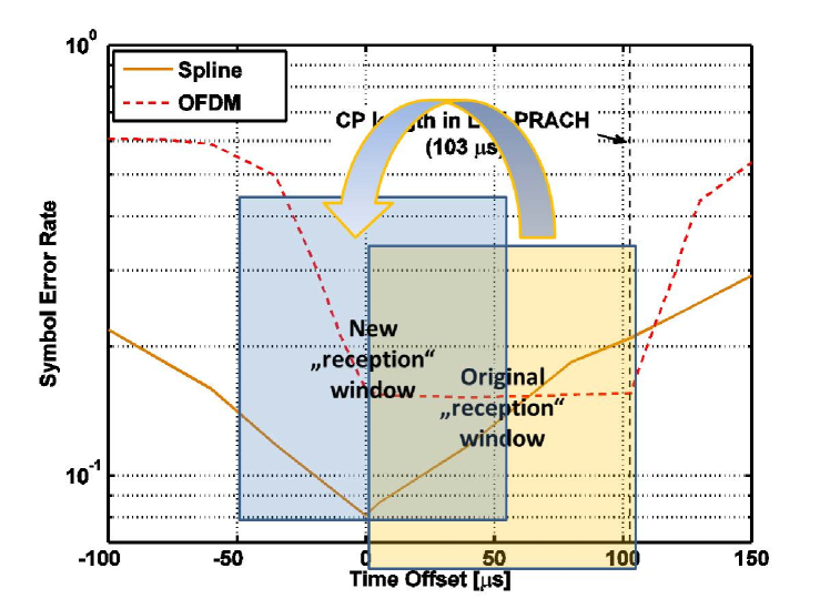
Figure 2: Illustration of autonomous timing advance (ATA). The spline waveform is in fact the candidate solution discussed in this paper and appears more robust to both symmetric time and frequency offsets. The curves depicted here are taken from Figure 16 in Section V-D and constitute one of our main results.

I-B Organization

The paper is organized as follows. In Section II, we describe the fundamentals of BFDM using Gabor theory and introduce the spline pulses. Then, in Section III, we present our approach to multiuser interference analysis in the context of highly asynchronous access and provide examples for the OFDM and spline waveforms. In Section IV, we deal with practical implementation issues for BFDM. In Section V, we investigate the performance of the proposed approach numerically and compare to standard LTE. In Section VI, we summarize our findings and draw some important conclusions.

II BFDM System Design

II-A Elements of Gabor signaling

Conventional OFDM and BFDM can be formulated as a pulse-shaped Gabor multicarrier scheme. For the time-frequency multiplexing we will adopt a two-dimensional index notation $n=(n_{1},n_{2})\in\mathbb{Z}^{2}$. Let $i$ denote the imaginary unit and $\mu=(\mu_{1},\mu_{2})$. The baseband transmit signal is then:

$$s(t)=\sum_{n\in{\mathcal{I}}}x_{n}\gamma_{n}(t)=\sum_{n\in{\mathcal{I}}}x_{n}({\bm{S}}_{\Lambda n}\,\gamma)(t),$$ (1)

where $({\bm{S}}_{\mu}\,\gamma)(t):=e^{i2\pi\mu_{2}t}\gamma(t-\mu_{1})$ is a time-frequency shifted version of the transmit pulse $\gamma$, i.e., $\gamma_{n}:={\bm{S}}_{\Lambda n}\,\gamma$ is shifted according to a lattice $\Lambda\mathbb{Z}^{2}$. The lattice is generated by the $2\times 2$ real generator matrix $\Lambda$ and the indices $n=(n_{1},n_{2})$ range over the doubly-countable set ${\mathcal{I}}\subset\mathbb{Z}^{2}$, referring to the data burst to be transmitted. The coefficients $x_{n}$ are the random complex data symbols at time instant $n_{1}$ and subcarrier index $n_{2}$ with the property $\mathbb{E}\{\bm{x}\bm{x}^{\ast}\}={\mathbb{I}}$ (from now on $\,\bar{\cdot}$ always denotes complex conjugate, $\cdot^{\ast}$ means conjugate transpose, and $\bm{x}=(\dots,x_{n},\dots)^{T}$). We will denote the linear time-variant channel by the operator $\bm{{\mathcal{H}}}$ and by $n(t)$ an additive distortion (a realization of a noise process).

In practice, $\Lambda$ is usually diagonal, i.e., $\Lambda=\text{diag}(T,F)$ and the time-frequency sampling density is related to the bandwidth efficiency (in complex symbols) of the signaling, i.e., $\epsilon:=|\det\Lambda^{-1}|=(TF)^{-1}$. The received signal is:

$$r(t)=(\bm{{\mathcal{H}}}s)(t)+n(t)=\int_{\mathbb{R}^{2}}\bm{\Sigma}(\mu)({\bm{S}}_{\mu}s)(t)d\mu+n(t),$$ (2)

with $\bm{\Sigma}:\mathbb{R}^{2}\rightarrow\mathbb{C}$ being a realization of the (causal) channel spreading function of finite support. In the wide-sense stationary uncorrelated scattering (WSSUS) assumption [11], the channel statistics is characterized by the second order statistics of $\bm{\Sigma}$, given as the scattering function $\bm{C}:\mathbb{R}^{2}\rightarrow\mathbb{R}_{+}$:

$$\mathbb{E}\{\bm{\Sigma}(\mu)\overline{\bm{\Sigma}(\mu^{\prime})}\}=\bm{C}(\mu)\delta(\mu-\mu^{\prime}).$$ (3)

Moreover, we assume $\mathbb{E}\{\bm{\Sigma}(\mu)\}=0$ and $\lVert\bm{C}\rVert_{1}=1$. To obtain the (unequalized) symbol $\tilde{x}_{m}$ on time-frequency slot $m\in{\mathcal{I}}$, the receiver projects on $g_{m}:={\bm{S}}_{\Lambda m}g$:

$$\tilde{x}_{m}:=\langle g_{m},r\rangle=\int\,e^{-i2\pi(\Lambda m)_{2}t}\overline{g(t-(\Lambda m)_{1})}\,r(t)dt,$$ (4)

using the ${\mathcal{L}}_{2}$ scalar product $\langle\cdot,\cdot\rangle:=\langle\cdot,\cdot\rangle_{{\mathcal{L}}_{2}}$. By introducing the elements

$$H_{m,n}:=\langle g_{m},\bm{{\mathcal{H}}}\gamma_{n}\rangle=\int_{\mathbb{R}^{2}}\Sigma(\mu)\langle g_{m},{\bm{S}}_{\mu}\gamma_{n}\rangle d\mu$$ (5)

of the channel matrix $H\in\mathbb{C}^{|{\mathcal{I}}|\times|{\mathcal{I}}|}$, the overall transmission can be formulated as a system of linear equations $\tilde{\bm{x}}=\bm{H}\bm{x}+\tilde{\bm{n}}$, where $\tilde{\bm{n}}=(\dots,\langle g_{m},n\rangle,\dots)^{T}$ is the vector of the projected noise. We use the AWGN assumption such that $\bm{\tilde{n}}$ is Gaussian random vector with independent components, each having variance ${\sigma^{2}}:=\mathbb{E}\{|r_{m},n\rangle|^{2}\}$. The diagonal elements

$$H_{m,m}=\int_{\mathbb{R}^{2}}\Sigma(\mu)e^{i2\pi(\mu_{1}(\lambda m)_{2}-\mu_{2}(\lambda m)_{1})}{\mathbf{A}}_{g\gamma}(\mu)d\mu.$$ (6)

Here,

$${\mathbf{A}}_{g\gamma}(\mu):=\langle g,{\bm{S}}_{\mu}\gamma\rangle=\int_{\mathbb{R}}g(t)\left({\bm{S}}_{\mu}\gamma\right)(t)dt$$ (7)

is the well known cross-ambiguity function of $g$ and $\gamma$.

Example 1.

A lattice can be described by a so-called generator matrix, which determines the geometry. For cp-OFDM, we can define the matrix

$$\Lambda=\begin{bmatrix}T+T_{cp}&0\\ 0&\frac{1}{T}\end{bmatrix}.$$ (8)

At the transmitter, the rectangular pulse

$$\gamma(t)=\frac{1}{\sqrt{T+T_{cp}}}\chi_{[-T_{[}[cp],T]}(t)$$ (9)

is used, with $\chi_{[-T_{[}[cp],T]}$ being the characteristic function of the interval $[-T_{[}[cp],T]$. The receiver obtains the complex symbol as

$$\tilde{x}_{m}=\int_{-\infty}^{\infty}g(t-(\Lambda n)_{1})e^{j2\pi(\Lambda n)_{2}t}dt,$$ (10)

using the rectangular pulse

$$g(t)=\frac{1}{\sqrt{T}}\chi_{[0,T]}(t)$$ (11)

for the removal of the CP.

II-B Completeness, Localization and Gabor Frames

In the following, we will collect some well-known statements on (bi-infinite) Gabor families $\mathcal{G}(\gamma,\Lambda):=\{\bm{S}_{\Lambda n}\gamma\}_{n\in\mathbb{Z}^{2}}$. A more detailed discussion of these concepts with respect to multicarrier transmission in doubly-dispersive channels can be found for example in [12] and [13]. Based on the generator matrix $\Lambda$, we can categorize the following regimes: we refer to critical sampling in case $\mathrm{det}(\Lambda)=1$, while $\mathrm{det}(\Lambda)<1$ and $\mathrm{det}(\Lambda)>1$ is called oversampling and undersampling of the time-frequency plane, respectively. Perfect reconstruction for any $\mathcal{I}\subseteq\mathbb{Z}^{2}$, i.e., $\langle g_{m},\gamma_{n}\rangle=\delta_{mn}$ for all $m,n\in\mathbb{Z}^{2}$, can be achieved if and only if $\mathrm{det}(\Lambda)\geq 1$. In this case, $g$ is called the dual (bi-orthogonal) pulse to $\gamma$ with respect to the lattice $\Lambda$. If $g=\gamma$, the Gabor family $\mathcal{G}(g,\Lambda)$ is an orthogonal basis for its span. However, a main consequence from the Balian Low Theorem is, that no well-localized prototype $\gamma$ (in both time and frequency) can generate a Gabor Riesz basis at $\mathrm{det}(\Lambda)=1$. Thus, any orthogonal or biorthogonal signaling at the critical density is ill-conditioned and will be highly sensitive with respect to either time or frequency shifts. Therefore, without further constraints on the data symbols, one has to operate in the undersampling regime in a practical scenario.

Let us now consider the adjoint lattice, generated by $\Lambda^{\circ}=\mathrm{det}(\Lambda)^{-1}\cdot\Lambda$, i.e., if $\mathcal{G}(\gamma,\Lambda)$ refers to undersampling, $\mathcal{G}(\gamma,\Lambda^{\circ})$ corresponds to oversampling. An important notion here is the concept of a Gabor frame, i.e. $\mathcal{G}(\gamma,\Lambda^{\circ})$ establishes a frame (for $L_{2}(\mathbb{R})$) if there are frame bounds $0<A_{\gamma}\leq B_{\gamma}<\infty$ such that:

$$A_{\gamma}\lVert f\rVert_{2}^{2}\leq\sum_{n\in\mathbb{Z}^{2}}\lvert\langle\bm{S}_{\Lambda^{\circ}n}\gamma,f\rangle\rvert^{2}\leq B_{\gamma}\lVert f\rVert_{2}^{2}$$ (12)

for all $f\in L_{2}(\mathbb{R})$. With $0<A_{\gamma}\leq B_{\gamma}<\infty$ we always mean here the best bounds. The Ron-Shen Duality now states that the Gabor family $\mathcal{G}(\gamma,\Lambda)$ is a Riesz basis for its span if and only if $\mathcal{G}(\gamma,\Lambda^{\circ})$ is a frame for $L_{2}(\mathbb{R})$. Furthermore, $\mathcal{G}(g,\Lambda^{\circ})$ is a tight frame $(A_{\gamma}=B_{\gamma})$ if and only if $\mathcal{G}(\gamma,\Lambda)$ is an orthogonal basis for its span. If $B_{\gamma}<\infty$ exists in (12) for the generator matrix $\Lambda$, the sequence of elements in $\mathcal{G}(\gamma,\Lambda)$ is called Bessel sequence. A straightforward argument shows that $B_{\gamma}$ is the maximal eigenvalue of the bi-infinite Gram matrix $G_{\gamma}$ with the components $(G_{\gamma})_{m,n}=\langle\gamma_{m},\gamma_{n}\rangle$. More details on these concepts in multicarrier transmission can be found in [14].

Example 2 ([15, Appendix A]).

The Bessel bound of cp-OFDM signaling is given by the operator norm of $S_{\gamma}$, which is equal to the largest eigenvalue of the Gram matrix $G_{\gamma}$, i.e.,

$$(G_{\gamma})_{m,n}=\delta_{m_{1},n_{1}}e^{-i\frac{\pi}{\epsilon}(n_{2}-m_{2})}\frac{\sin\frac{\pi}{\epsilon}(n_{2}-m_{2})}{\frac{\pi}{\epsilon}(n_{2}-m_{2})},$$ (13)

where $\epsilon=\frac{T_{u}}{T_{u}+T_{cp}}$. This is a Toeplitz matrix in the frequency slots $m_{2}$ and $n_{2}$ generated by:

$$\phi(\omega) =\sum_{n=-\infty}^{\infty}e^{j\pi(2\omega-\frac{1}{\epsilon})n}\frac{\sin\frac{\pi}{\epsilon}n}{\frac{\pi}{\epsilon}n}=1+\frac{2\epsilon}{\pi}\sum_{n=1}^{\infty}\frac{\cos\pi(2\omega-\frac{1}{\epsilon})n\cdot\sin\frac{\pi}{\epsilon}n}{n}$$ (14)

$$=1+\epsilon-\epsilon\left[\left(\frac{1}{\epsilon}-\omega\right)\mathrm{mod}1+\omega\right]=\epsilon\left(\lfloor\frac{1}{\epsilon}-\omega\rfloor+1\right).$$ (15)

Using this, the Bessel bound for cp-OFDM can be upperbounded by $B_{\gamma}=2$. However, of course this is only the worst-case estimation. Interestingly, by contrast, the Bessel bound $B_{g}$ for the receive ”frame” is exactly unity, i.e., $B_{g}=1$.

II-C Spline-based Gabor Signalling

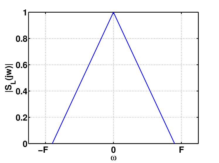
Figure 3: Illustration of 1^st order spline function. It is the result of a convolution of two 0^th order rectangular pulses.

As mentioned before, the used pulses $g$ and $\gamma$ play a key role and should therefore be carefully designed. As we consider a BFDM approach, we generate the transmit pulse $g$ according to system requirements and compute the receive pulse $\gamma$ as the canonical dual (biorthogonal) pulse. For this, we use a method already applied, for example, in [12]. Briefly explained, bi-orthogonality in a stable sense means that $g$ should generate a Gabor Riesz basis and $\gamma$ generates the corresponding dual Gabor Riesz basis. From the Ron-Shen duality principle [16] follows that $\gamma$ has the desired property if it generates a Gabor (Weyl-Heisenberg) frame on the so called adjoint time-frequency lattice and that frame is dual to the frame generated by $g$. This can be achieved with the $S^{-1}$-trick explained in [17]. Side effects such as spectral regrowth due to periodic setting when calculating the bi-orthogonal pulses are negligible.

As a rough and well-known guideline for well-conditioning of this procedure, the ratio of the time and frequency pulse widths (variances) $\sigma_{t}$ and $\sigma_{f}$ should be approximately matched to the time-frequency grid ratio

$$\frac{T}{F}\approx\sqrt{\frac{\sigma_{t}}{\sigma_{f}}},$$ (16)

and this should also be in the order of the channel’s dispersion ratio [12]. However, since we focus on a design being close to the conventional LTE PUSCH and PRACH, of this rule, we consider only (16) here.

We propose to construct the pulse $g$ based on the B-splines in the frequency domain, see Figure 3. $B$-splines have been investigated in the Gabor (Weyl-Heisenberg) setting for example in [18]. The main reason for using the B-spline pulses is that convolution of such pulses have excellent tail properties with respect to the $L_{1}$-norm, which is beneficial with respect to the overlap of PRACH to the PUSCH symbols. We also believe that they trade off well the time offset for the frequency offset performance degradation but this is part of further on-going investigations and beyond the conceptional approach here. Because of its fast decay in time, we choose a second order B-spline (the ”tent”-function) in frequency domain, given by

$$B_{2}(f) =B_{1}(f)\ast B_{1}(f),\;\text{where}$$ (17)

$$B_{1}(f) :=\chi_{[-\frac{1}{2},\frac{1}{2}]}(f)$$ (18)

(and $\ast$ denotes convolution). It has been shown in [18] that $B_{2}(f)$ generates a Gabor frame for the $(a,b)$-grid (translating $B_{2}$ on $a\mathbb{Z}$ and its Fourier transform on $b\mathbb{Z}$) if (due to its compact support) $a<2$ and $b\leq 1/2$, and fails to be frame in the region:

$$\{a\geq 2,\,b>0\}\cup\{a>0,1<b\in\mathbb{N}\}.$$ (19)

Recall, that by Ron-Shen duality [16] it follows that the same pulse prototype $B_{2}(f)$ generates a Riesz basis on the adjoint $(\frac{1}{b},\frac{1}{a})$-grid. In our setting, we will effectively translate the frequency domain pulse $B_{2}(f)$ by half of its support, which corresponds to $\frac{1}{b}=1$, and we will use $\frac{1}{b}\cdot\frac{1}{a}=\frac{5}{4}=1.25$ (see here also Table I) such that $a=\frac{4}{5}$. Therefore, it follows that our operation point $(a,b)=(\frac{4}{5},1)$ is not in any of two explicit $(a,b)$-regions given above. But for $1.1\leq a\leq 1.9$ a further estimate has been computed explicitly for $B_{2}(f)$ [18, Table 2.3 on p.560], ensuring the Gabor frame property up to $b\leq 1/a$. Finally, we like to mention that for $ab\leq 1/2$ the dual prototypes can be expressed again as finite linear combinations of $B$-splines, i.e., explicit formulas exists in this case [19]. Note that we can choose a larger grid in the frequency domain and set $b\leq 1/2$ so that $a=8/5$, which is a frame (so that the spline is a Riesz basis). Hence, due to the spectral efficiency constraint with increasing $1/b$, we also decrease the time domain grid such that, necessarily, at some point $a\geq 2$ (in the dual domain) and so we do not get a Riesz basis (or a frame in the dual domain).

In practice, $g$ has to be of finite duration, i.e., the transmit pulse in time domain will be smoothly truncated:

$$g(t)=\left(\frac{\mathrm{sin}(B\pi t)}{B\pi t}\right)^{2}\chi_{[c,d]}(t),$$ (20)

where $B$ is chosen equal to $F$ and parameters $c$ and $d$ align the pulse within the transmission frame. Theoretically, a (smooth) truncation in (20) would imply again a limitation on the maximal frequency spacing $B$ [20]. Although the finite setting is used in our application, the frame condition (and therefore the Riesz basis condition) is a desired feature since it will asymptotically ensure the stability of the computation of the dual pulse $\gamma$ and its smoothness properties.

To observe the pulse’s properties regarding time-frequency distortions, we depict in Figure 4 the discrete cross-ambiguity function $A_{g,\gamma}$ between pulse $g$ and $\gamma$.

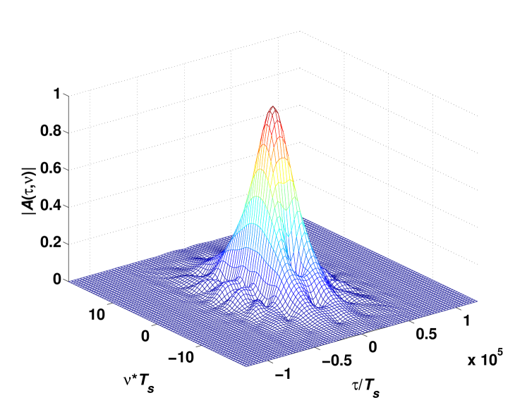
Figure 4: The cross–ambiguity function $A_{g,\gamma}(\nu,\tau)$ for transmit and receive pulses on the frame length of $4\,ms$.

It can be observed that its value at the neighboring symbol is already far below $10^{-3}$. Obviously, the bi-orthogonality condition states $A_{g,\gamma}(kT,lF)=\delta_{k,0}\delta_{t,0}$ and ensures perfect symbol recovery in the absence of channel and noise. However, the sensibility with respect to time-frequency distortions is related to the slope shape of $A_{g,\gamma}$ around the grid points. Depending on the loading strategies for these grid points it is possible to obtain numerically performance estimates using, for example, the integration methods presented in [12].

Let us introduce a parameter $\alpha$ to scale the width of the spline pulse in frequency. Choosing a large pulse width $\alpha$ has the disadvantage of an increasing value of $B_{g}$ in (41). This is illustrated in Figure 5. It shows the upper frame constant $B_{g}$ for the transmit pulse $g$ vs. its pulse width $\alpha$. The frame constant is thereby calculated using the LTFAT toolbox [21]. It can be observed that $B_{g}$ has its smallest value around $\alpha=0.85$, however, it never reaches the lower bound $B_{g}=1$.

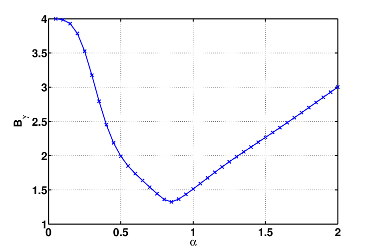
Figure 5: Upper frame constant $B_{\gamma}$ over $\alpha$. A minimum of this function can be observed around $1$ (more precisely, at $\alpha=0.85$), while for increasing and, even more, for decreasing values of alpha the value of $B_{\gamma}$ increases.

III Multiuser Interference Analysis

III-A A general approach

Our system model has to capture that many users each occupy a small number of subcarriers and each of them asynchronously (in time and frequency or both) access this resource in an uncoordinated fashion. For a particular time-frequency slot $m=(m_{1},m_{2})$, we will denote the (random) channel operator as $\bm{{\mathcal{H}}}(m)$ and the asynchronism as $\mathcal{D}\left(m\right)$. We assume that $\bm{{\mathcal{H}}}(m)$ can be estimated using channel estimation procedure while $\mathcal{D}\left(m\right)$ cannot. Writing the received complex symbol $\tilde{x}_{m}$ in the absence of additive noise yields

$$\tilde{x}_{m}=\overline{H}_{m}x_{m}+\overbrace{(H_{m,m}-\overline{H}_{m})}^{\Delta_{m}}x_{m}+\underbrace{\sum_{n\in\mathcal{I},n\neq m}H_{m,n}x_{n}}_{\text{ICI}}$$ (21)

where we defined $\overline{H}_{m}:=\mathbb{E}_{|\mathcal{H}}\{H_{m,m}\}$, i.e., the mean value conditioned on a fixed channel $\mathcal{H}$. Thus, the transmitted symbol $x_{m}$ will be multiplied by a constant and disturbed by two zero mean random variables (RV), $\Delta_{m}$ and ICI. The first RV $\Delta_{m}$ represents a distortion, which comes from the randomness of $\mathcal{D}\left(m\right)$, the second term ICI represents both. The mean power of both contributions, conditioned on a fixed channel $\bm{\mathcal{H}}$, are $D_{m}:=\mathbb{E}_{|\mathcal{H}}\{|\Delta_{m}|^{2}\}=P_{m}-|\overline{H}_{m}|^{2}$ where $P_{m}:=\mathbb{E}_{|\mathcal{H}}\{|H_{m,m}|^{2}\}$ and $I_{m}:=\mathbb{E}\{|\text{ICI}|^{2}\}$. Each element of the distortion sum $\sum_{n\neq m}H_{m,n}x_{n}$ is given by:

$$H_{m,n}=\langle g_{m},\mathcal{D}\left(n\right)\bm{{\mathcal{H}}}(n)\gamma_{n}\rangle.$$ (22)

Remark 2.

Notably, even if $\mathcal{D}\left(n\right)$ is the identity (synchronous access) $\tilde{x}_{m}$ is affected by all other individual contributions where the operators depend also on the index $n=(n_{1},n_{2})$. Hence, the performance for individual slots will be quite different, which complicates the situation, and no analytical approach is available so far! If all $\mathcal{D}\left(n\right)$ and $\bm{{\mathcal{H}}}(n)$ are independent of $n$, standard analysis can be used [12].

To find a tractable way, we consider the following approach: We assume that the $H_{m,m}$ can be estimated, and we consider the distortion sum $\sum_{n\neq m}H_{m,n}x_{n}$ averaged over all the subcarriers $m$. Obviously, this will average out individual interference for a specific subcarrier, but we can assume that these interference terms do not differ much. Individual performance is then measured by $H_{m,m}$ only! Then, we average over the random operators $\mathcal{D}\left(n\right)$ and $\bm{{\mathcal{H}}}(n)$. Let us first consider the sums:

$$\sum_{m}\sum_{n\neq m}\left|H_{m,n}\right|^{2} =\sum_{m}\sum_{n\neq m}\left|\langle g_{m},\mathcal{D}\left(n\right)\bm{{\mathcal{H}}}(n)\gamma_{n}\rangle\right|^{2}\newline$$ (23)

$$=\sum_{n}\sum_{m}\left|\langle g_{m},\mathcal{D}\left(n\right)\bm{{\mathcal{H}}}(n)\gamma_{n}\rangle\right|^{2}-\sum_{m}\left|\langle g_{m},\mathcal{D}\left(m\right)\bm{{\mathcal{H}}}(m)\gamma_{m}\rangle\right|^{2}\newline$$ (24)

$$\leq B_{g}E_{g}\sum_{n}\left\|\mathcal{D}\left(n\right)\bm{{\mathcal{H}}}(n)\gamma_{n}\right\|_{2}^{2}-\sum_{m}\left|\langle g_{m},\mathcal{D}\left(m\right)\bm{{\mathcal{H}}}(m)\gamma_{m}\rangle\right|^{2}\newline$$ (25)

$$=B_{g}E_{g}\sum_{n}\left\|\mathcal{D}\left(n\right)\bm{{\mathcal{H}}}(n)\gamma_{n}\right\|_{2}^{2}-\sum_{m}\left|H_{m,m}\right|^{2}.$$ (26)

Here, $B_{g}$ is the Bessel bound of the Gabor family $\mathcal{G}(g,\Lambda)$. In the last step, we see that only the ”action” of the operators $\{\mathcal{D}\left(n\right),\bm{{\mathcal{H}}}(n)\}$ on $\gamma$ is relevant. We have set without loss of generality $||\gamma||_{2}^{2}=1$ and $1\leq||g||_{2}^{2}\leq E_{g}$ (typically $E_{g}\approx 1$). Next, we compute the expectations and we use $D_{m}=P_{m}-|\overline{H}_{m}|^{2}$:

$$\mathbb{E}\sum_{m}\sum_{n\neq m}\left|H_{m,n}\right|^{2}+\mathbb{E}\sum_{m}D_{m}\newline$$ (27)

$$\leq B_{g}E_{g}\sum_{n}\mathbb{E}\left\|\mathcal{D}\left(n\right)\bm{{\mathcal{H}}}(n)\gamma_{n}\right\|_{2}^{2}-\sum_{m}\mathbb{E}\left|H_{m,m}\right|^{2}+\mathbb{E}\sum_{m}D_{m}\newline$$ (28)

$$\leq B_{g}E_{g}\sum_{n}\mathbb{E}\left\|\mathcal{D}\left(n\right)\bm{{\mathcal{H}}}(n)\gamma_{n}\right\|_{2}^{2}-\mathbb{E}\sum_{m}(P_{m}-D_{m})\newline$$ (29)

$$=B_{g}E_{g}\sum_{n}\mathbb{E}\left\|\mathcal{D}\left(n\right)\bm{{\mathcal{H}}}(n)\gamma_{n}\right\|_{2}^{2}-\sum_{m}\mathbb{E}|\overline{H}_{m}|^{2}.$$ (30)

We assume that the asynchronisms cannot increase the received power. For the first term, we estimate

$$\sum_{n}\mathbb{E}\left\|\mathcal{D}\left(n\right)\bm{{\mathcal{H}}}(n)\gamma_{n}\right\|_{2}^{2}\leq\sum_{n}\mathbb{E}\lVert\bm{\mathcal{H}}\left(n\right)\gamma_{n}\rVert_{2}^{2}\leq\sum_{n}\lVert\bm{C}_{n}\rVert_{1},$$ (31)

according to (3). It remains to bound the second term

$$\mathbb{E}|\overline{H}_{m}|^{2}=\mathbb{E}\left||\mathbb{E}_{|\mathcal{H}}\langle g_{m},\mathcal{D}\left(m\right)\bm{{\mathcal{H}}}(m)\gamma_{m}\rangle\right|^{2}$$ (32)

for some $m$. For $a,b\in\mathbb{R}^{2}$, we abbreviate $[a,b]:=a_{1}b_{2}-a_{2}b_{1}$ (the symplectic form). Define now the following function:

$$s_{m}(\mu) :=\mathbb{E}_{|\mathcal{H}}\langle g_{m},\mathcal{D}\left(m\right){\bm{S}}_{\mu}\gamma_{m}\rangle$$ (33)

$$=e^{-j2\pi[\mu,\Lambda m]}\mathbb{E}_{|\mathcal{H}}\langle g,{\bm{S}}_{\Lambda m}^{\ast}\mathcal{D}\left(m\right){\bm{S}}_{\Lambda m}{\bm{S}}_{\mu}\gamma\rangle,$$ (34)

which essentially contains the distortion of the $\mu$th contribution in terms of the pulses conjugated by $\bm{S}_{\Lambda m}$, i.e., ”shifted” to TF-slot $m$ in the time-frequency plane. For a fixed channel $\bm{\Sigma}$, we have $\overline{H}_{m}=\langle\bm{\Sigma},s_{m}\rangle$ and on average, with respect to $\bm{{\mathcal{H}}}(m)$, we have:

$$\mathbb{E}\{|\overline{H}_{m}|^{2}\}=\langle\bm{C}_{m},|s_{m}|^{2}\rangle.$$ (35)

Hence, altogether we have the following upper bound on the total expected distortion:

$$\mathbb{E}\sum_{m\in\mathcal{I}}(I_{m}+D_{m})\leq\sum_{m\in\mathcal{I}}(E_{g}B_{g}\lVert\bm{C}_{m}\rVert_{1}-\langle\bm{C}_{m},|s_{m}|^{2}\rangle).$$ (36)

Let us fix the normalization such that $\sum_{m\in\mathcal{I}}\lVert\bm{C}_{m}\rVert_{1}/|\mathcal{I}|=1$. Hence, averaging over $\mathcal{I}$, we have proved the following theorem.

Theorem 1.

Suppose $\lVert\gamma_{m}\rVert_{2}^{2}=1$ (without loss of generality)$,\lVert g_{m}\rVert_{2}^{2}=E_{g}$ such that $\langle\bm{g}_{m},\gamma_{m}\rangle=1$ (perfect reconstruction in noiseless case). The average distortion power per subcarrier is upperbounded by

$$\frac{1}{|\mathcal{I}|}\mathbb{E}\sum_{m\in\mathcal{I}}(I_{m}+D_{m})\leq E_{g}B_{g}-\frac{1}{|\mathcal{I}|}\sum_{m\in\mathcal{I}}\langle\bm{C}_{m},|s_{m}|^{2}\rangle,$$ (37)

where:

$$s_{m}(\cdot)=\mathbb{E}_{|\mathcal{H}}\langle g_{m},\mathcal{D}\left(m\right){\bm{S}}_{(\cdot)}\gamma_{m}\rangle.$$

Example 3.

As a special case, assume now a deterministic time-frequency shift $\mathcal{D}\left(m\right)=\bm{S}_{\nu(m)}$. This distortion is non-random and energy preserving, i.e., $\lVert\mathcal{D}\left(m\right)g_{m}\rVert_{2}=\lVert g_{m}\rVert_{2}$. Evaluating the function $s_{m}$ in (33) gives:

$$s_{m}(\mu(m)) =e^{-i2\pi[\mu(m),\Lambda m]}\langle g,{\bm{S}}_{\Lambda m}^{\ast}{\bm{S}}_{\nu(m)}{\bm{S}}_{\Lambda m}{\bm{S}}_{\mu(m)}\gamma\rangle=e^{-i2\pi[\nu(m)+\mu(m),\Lambda m]}\langle g,{\bm{S}}_{\nu(m)}{\bm{S}}_{\mu(m)}\gamma\rangle$$ (38)

$$=e^{-i2\pi\left([\nu(m)+\mu(m),\Lambda m]+\nu_{1}(m)\mu_{2}(m)\right)}\langle g,{\bm{S}}_{\nu(m)+\mu(m)}\gamma\rangle$$ (39)

$$=e^{-i2\pi\left([\nu(m)+\mu(m),\Lambda m]+\nu_{1}(m)\mu_{2}(m)\right)}{\mathbf{A}}_{g\gamma}(\nu(m)+\mu(m)).$$ (40)

Hence, in the AWGN case we have:

$$\frac{1}{\left|{\mathcal{I}}\right|}\mathbb{E}\sum_{m\in\mathcal{I}}(I_{m}+D_{m})\leq E_{g}B_{g}-\frac{1}{\left|{\mathcal{I}}\right|}\sum_{m\in\mathcal{I}}|{\mathbf{A}}_{g\gamma}(\nu(m))|^{2}.$$ (41)

III-B OFDM

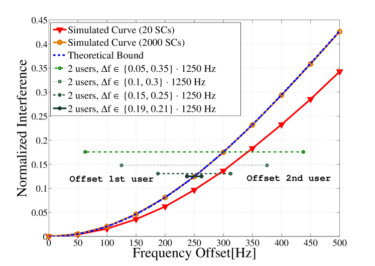
Figure 6: Simulated interference over frequency offset using different numbers of subcarriers, compared to theoretical bound. In addition, the behavior of the two-user case is illustrated, where each user gets half of the available subcarriers and has a different frequency offset. The (aggregate) interference converges to the value of the bound when the differences between the two offsets, which are centered around $0.2\cdot 1250Hz$, and their average become smaller.

The cross ambiguity function for $\gamma$ and $g$, as introduced in (7), can be compactly written as (see [15])

$${\mathbf{A}}_{g\gamma}(\nu) =\frac{\sin\pi\nu_{2}(T_{u}-|[\nu_{1}]_{\text{cp}}|)}{\pi\nu_{2}T_{u}}e^{j(\phi_{0}-\pi\nu|[\nu_{1}]_{\text{cp}}|)}\chi_{[-T_{u},T_{u}]}([\nu_{1}]_{\text{cp}})$$ (42)

$$={\mathbf{A}}_{gg}(([\nu_{1}]_{\text{cp}},\nu_{2})),$$ (43)

where the phase $\phi_{0}=\pi\nu T_{u}$ is related to our choice of time origin and

$$[\cdot]_{\text{cp}}\ :\tau\rightarrow[\tau]_{\text{cp}}=\begin{cases}\tau&\tau\leq 0,\\ 0&0<\tau<T_{cp},\\ \tau-T_{cp}&\tau\geq T_{cp}.\end{cases}$$ (44)

The signal quality in the presence of time- and frequency shifts can now be directly obtained from (43). Apart from $[\cdot]_{\text{cp}}$ and $\sqrt{\epsilon}$ (the loss in mean signal amplitude due to the CP) (43) agrees with the well known auto ambiguity function $\mathbf{A}_{gg}$ for a rectangular pulse $g$ of width $T_{u}$.

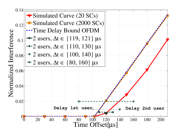
Figure 7: Simulated interference over time offsets using different numbers of subcarriers, compared to theoretical bound.

Let us also consider time-invariant channels, i.e., (distributional) spreading functions of the form $\bm{\Sigma}(\mu)=h(\mu_{1})\delta(\mu_{2})$. Here, $h$ is called the channel impulse response. If the system exhibits a timing offset $\nu_{1}$ with $[\nu_{1}+{\tau_{d}}]_{\text{cp}}=0$ only, the time dependency in the cross ambiguity function cancels, thus

$$s_{m}((\nu_{1},0))=e^{-i2\pi\nu_{1}m_{2}/T_{u}}{\mathbf{A}}_{g\gamma}((\nu_{1},0))\newline =e^{-i2\pi\hat{\nu}_{1}m_{2}/\epsilon}{\mathbf{A}}_{g\gamma}((\nu_{1},0))=e^{i[\phi_{0}-2\pi\hat{\nu}_{1}m_{2}/\epsilon]}$$ (45)

and only phase rotations occur (normally corrected by channel estimation and equalization). Contrary to this, time offsets with $[\nu_{1}+{\tau_{d}}]_{\text{cp}}\neq 0$ cause interference. For frequency offsets, interference occurs immediately. For the case $[\nu_{1}+{\tau_{d}}]_{\text{cp}}=0$, the following relation holds:

$$\langle\bm{\Sigma},s_{m}\rangle=e^{-i2\pi[\hat{\nu},m]/\epsilon}\frac{\sin\pi\hat{\nu}_{2}}{\pi\hat{\nu}_{2}}e^{i\phi_{0}}\,\hat{h}(m_{2}/T_{u}).$$ (46)

Obviously, the frequency offset $\hat{\nu}_{2}$ (the time offset $\hat{\nu}_{1}$) induces a rotating phase over the time slots $l$ (over frequency slots $k$) as one would expect.

Finally, we need the Bessel bound (by contrast to transmit pulse) for the receive pulse $g$, which is $B_{g}=1$ (see Example 2), and the energy constant, which is $E_{g}=\epsilon$, so that altogether

$$\frac{1}{\left|{\mathcal{I}}\right|}\mathbb{E}\sum_{m}(I_{m}+D_{m})\leq\epsilon-\frac{1}{\left|{\mathcal{I}}\right|}\sum_{m\in\mathcal{I}}\frac{\sin^{2}(\pi\nu_{2}^{m}(T_{u}-|[\nu_{1}^{m}]_{\text{cp}}|))}{(\pi\nu_{2}^{m}T_{u})^{2}}\chi_{[-T_{u},T_{u}]}([\nu_{1}^{m}]_{\text{cp}}).$$ (47)

III-B1 Evaluation

First, we consider only frequency offsets with no additional delay in time. Figure 6 shows a comparison of this interference bound with simulated curves at different numbers of subcarriers. It can be observed that with an increasing number of subcarriers considered, the interference curve gets closer to the theoretical bound. In case of 200, or even more 20000, subcarriers, the simulations match the bound almost perfectly.

The described curves are based on a single frequency offset only, which is the same for all subcarriers. However, Figure 6 additionally illustrates the behavior in case of multiple different offsets. For the sake of illustration, we demonstrate the case of two offsets here, where each offset applies to an equal share of the available subcarriers. It can be observed that with decreasing difference in the offsets, the resulting interference level gets closer to value of the bound at the corresponding average of the offsets.

Let us now consider the case of time delays. Figure 7 compares the interference caused by the asynchronous mode of operation to that predicted by the theoretical bound. Again, it can be observed that the numerical results converge to the bound when increasing the number of subcarriers. Note that the CP length is 103ms; an smaller offset does not produce any interference (however, negative delays do, which is not depicted here).

III-C Spline-based modulation

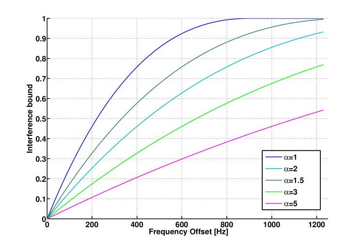
Figure 8: Interference bound for spline waveform based over frequency offset for increasing values of alpha. Note that $B_{\gamma}=1$ is assumed in all curves.

Let us now investigate the influence of time and frequency offsets on the spline-based waveform, as carried out for OFDM in Section III-B. In order to obtain a bound on the influence of time or frequency offsets, we need to evaluate the cross-ambiguity function $A_{g\gamma}$. For this, the dual pulse has to be taken into account. However, since this is not desirable, simple estimates of this function are needed. For this purpose, consider the following bound. Define $\gamma_{\mu}:=\bm{S}_{\mu}\gamma$ and $\gamma_{\nu}:=\bm{S}_{\nu}\gamma$, and using $\langle g,\gamma\rangle=1$ and $\lVert g\rVert_{2}=E_{g}$:

$$|A_{g\gamma}(\mu)| =|\langle g,\gamma_{\mu}-\gamma+\gamma\rangle|$$ (48)

$$=|1+\langle g,\gamma_{\mu}-\gamma\rangle|=|1+\langle g,\gamma_{\mu}-\gamma_{\nu}+\gamma_{\nu}-\gamma\rangle|$$ (49)

$$\geq 1-|\langle g,\gamma_{\mu}-\gamma_{\nu}\rangle|-|\langle g,\gamma_{\nu}-\gamma\rangle|$$ (50)

$$\geq 1-E_{g}\lVert\gamma_{\mu}-\gamma_{\nu}\rVert_{2}-E_{g}\lVert\gamma_{\nu}-\gamma\rVert_{2},$$ (51)

where the RHS constitutes a similarity measure for $\gamma$. Let us take $\mu=(\Delta t,\Delta\omega)$ and $\nu=(0,\Delta\omega)$ and it follows:

Theorem 2.

Suppose $\lVert\gamma_{m}\rVert_{2}^{2}=1$ (without loss of generality)$,\lVert g_{m}\rVert_{2}^{2}=E_{g}$ such that $\langle\bm{g}_{m},\gamma_{m}\rangle=1$ (perfect reconstruction in noiseless case). Then

$$|A_{g\gamma}(\mu)|\geq 1-\lVert\gamma-\gamma(\cdot-\Delta t)\rVert_{2}-\lVert\hat{\gamma}-\hat{\gamma}(\cdot-\Delta\omega)\rVert_{2},$$ (52)

where $\hat{\gamma}$ denotes the Fourier transform of $\gamma$.

From this, we get by standard analysis the following approximation for frequency offsets:

$$A_{g\gamma}((0,\Delta\omega))\geq 1-\frac{\sqrt{3}\Delta\omega T}{2\pi\alpha}\sqrt{\left(1-\frac{\Delta\omega T}{2\pi\alpha}\right)}.$$ (53)

Using this approximation we can calculate the interference part in (41). Figure 8 illustrates the behavior of the spline waveform with different pulse widths $\alpha$. It can be observed, that the interference decreases with increasing pulse width. Similar to frequency offsets, we can derive:

$$A_{g\gamma}((\Delta t,0))\geq 1-\frac{2\pi\alpha\Delta t}{\sqrt{20}T}.$$ (54)

III-C1 Evaluation

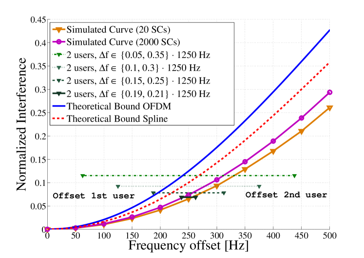
Figure 9: Simulated interference and interference bound vs. frequency offsets for the spline waveform. Numerical results for different numbers of subcarriers are shown. To foster an easy comparison, the interference bound for OFDM is also depicted.

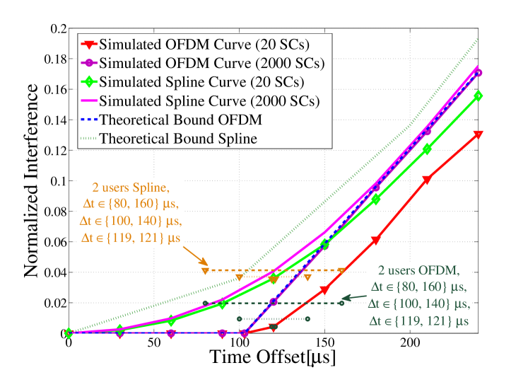
Figure 10: Simulated interference and interference bound vs. time offset for the spline waveform. Numerical results for different numbers of subcarriers are shown. To foster an easy comparison, the interference bound for OFDM is also depicted.

In Figure 9, we show the simulated interference of the spline waveform together with the corresponding bound based on a numerical computation of $A_{g\gamma}$ in (41) for frequency offsets. In addition, the figure again shows also the interference bound for OFDM. While, the results for the spline waveform indicate lower interference than in the OFDM case, the bound appears to be less tight, even with large numbers of subcarriers.

Let us now consider the case of time offsets. Figure 10 depicts the interference bound, again based on a numerical calculation of $A_{g\gamma}$ in (41) and the simulated interference vs. a time offset for the spline waveform. To allow an easy comparison, the bound for OFDM is also shown. It should be noted that although the results do not outperform OFDM for the positive delays considered in Figure 10, the behavior is different for negative delays. In Figure 11, we show the influence of negative delays, where the benefits of the spline waveform become obvious.

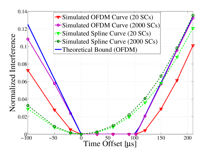
Figure 11: Simulated interference and interference bound vs. negative and positive time offsets for OFDM and spline waveform. Numerical results for different numbers of subcarriers are shown. To foster an easy comparison, the interference bound for OFDM is also depicted.

IV Practical Implementation

In the following, let $T_{s}$ denote the sampling period, which is equal to $1/f_{s}$, with $f_{s}$ being the sampling frequency. In the following discrete model, we let all time indices be multiples of $T_{s}$ and frequency indices be multiples of $F$. Furthermore, we use $N$ to denote the discrete counterpart of the symbol duration and submit $K$ symbols. Let $N_{\mathrm{FFT}}$ be the FFT-length in D-PRACH. Note, for some numerical reasons $N_{\mathrm{FFT}}$ must divide $NK$. In order to be compliant with 4G, we set $TF=1.25$. Note that efficient implementations are available in literature [22].

IV-A Transmitter

For the pulse shaped PRACH, additional processing is needed, compared to standard OFDM. In contrast to standard processing, we process more than one symbol interval, even if we use only one symbol to carry the preamble. A pulse $g$ is used to shape the spectrum of the preamble signal (which is constructed from a Zadoff-Chu (ZC) sequence [23]), e.g., to allow the use of PRACH guard bands with acceptable interference. Let $P$ be the length of pulse $g$. We extend the output signal $s[n]$ after the inverse FFT (IFFT) stage by repeating it and taking modulo $P$ to get the same length as the pulse $g$. Given $K$ symbols, each symbol $s_{k}[n]$ is pointwise multiplied by the shifted pulse $g$ and superimposed by overlap and add, such that we get the baseband pulse shaped D-PRACH transmit signal as:

$$s[n]=\sum_{k=0}^{K-1}s_{k}[n]g[n-kN].$$ (55)

In greater detail, this can be written as

$$s[n]=\beta\sum_{k=0}^{K-1}\sum_{l\in\mathcal{F}_{1}\cap\mathcal{F}_{2}}\tilde{X}_{k,l}\;g[n-kN]e^{j\frac{2\pi nl}{N_{\mathrm{FFT}}}},$$ (56)

where $\tilde{X}_{k,l}$ is the Fourier transformed preamble signal (which is constructed from Zadoff-Chu (ZC) root sequences [23] in LTE-A) occupying subcarriers $l\in\mathcal{F}_{1}$ of length $N_{\mathrm{ZC}}$ and the actual data occupying subcarriers $l\in\mathcal{F}_{2}$ at the $k$-th symbol, and $\beta$ is an amplitude scaling factor for normalizing the transmit power.

IV-B Receiver

Assuming an AWGN channel and one user transmitting its preamble signal on the PRACH, the base station obtains the superposition of data bearing signals, preamble signal, and noise as

$$r[n]=s_{\mathrm{PU}}[n]+s_{\mathrm{PR}}[n]+n_{0}[n],$$ (57)

where $s_{\mathrm{PU}}$ is the PUSCH data transmit signals, $s_{\mathrm{PR}}$ is the PRACH preamble transmit signal, and $n_{0}$ is Gaussian noise.

The only difference of our BFDM receiver to the standard OFDM PRACH receiver is the processing before the FFT. While in standard PRACH processing the CP has to be removed from the received signal $r_{\mathrm{PR}}[n]$, in our BFDM receiver, an operation to invert the (transmitter side) pulse shaping is carried out. To be more precise, the $K$ symbols of the received signal $r_{\mathrm{PR}}[n]$ are pointwise multiplied by the shifted bi-orthogonal pulse $\gamma$, such that we have

$$r_{k}^{\gamma}[n]=r_{k}[n]\gamma^{\ast}[n-kN].$$ (58)

Subsequently, some kind of prealiasing operation is applied to each windowed $r_{k}^{\gamma}[n]$, i.e.,

$$\tilde{r}_{k}^{\gamma}[n]=\sum_{l=0}^{P/N_{\mathrm{FFT}}-1}r_{k}^{\gamma}[n-lN_{\mathrm{FFT}}],$$ (59)

such that we obtain the Fourier transformed preamble sequence at the $k$-th symbol and $l$-th subcarrier after the FFT operation

$$\tilde{Y}_{k,l}=\sum_{n=0}^{N_{\mathrm{FFT}}-1}\tilde{r}_{k}^{\gamma}[n]e^{-\frac{j2\pi nl}{N_{\mathrm{FFT}}}}.$$ (60)

Although we do not employ a CP as in standard PRACH, the time-frequency product of $TF=1.25$ allows the signal to have guard regions in time and frequency as well. This time-frequency guard regions and the overlapping of the pulses evoke the received signal to be cyclostationary [24], which gives the same benefit as the cyclostationarity made by CP. Furthermore, it is also shown in [24], that the bi-orthogonality condition of the pulses is sufficient for the cyclostationarity and makes it possible to estimate the symbol timing offset from its correlation function.

IV-C User Detection

IV-C1 Preamble generation

The preamble is constructed from a ZC sequence as

$$x_{u}[m]=\exp\left\{-j\frac{\pi um(m+1)}{N_{\mathrm{ZC}}}\right\},0\leq m\leq N_{\mathrm{ZC}}-1,$$ (61)

where $u$ is the root index and $N_{\mathrm{ZC}}$ is the length of the preamble sequence, which is fixed for all users. Here, we consider the case of contention based RACH, where every user wanting to send a preamble chooses a signature randomly from the set of available signatures $\mathcal{S}=\{1,...,64-N_{\mathrm{cf}}\}$, with $N_{\mathrm{cf}}$ being a given number of reserved signatures for contention free RACH. Every element of $\mathcal{S}$ is assigned to index $(u,v)$, such that the preamble for each user is obtained by cyclic shifting the $u$-th Zadoff-Chu sequence according to $x_{u,v}[m]=x_{u}[(m+v\,N_{\mathrm{CS}})\,\mathrm{mod}\,N_{\mathrm{ZC}}]$, where $v=1,...,\left\lfloor\frac{N_{\mathrm{ZC}}}{N_{\mathrm{CS}}}\right\rfloor$ is the cyclic shift index and $N_{\mathrm{CS}}$ is the cyclic shift size. Since only $V=\left\lfloor\frac{N_{\mathrm{ZC}}}{N_{\mathrm{CS}}}\right\rfloor$ preambles can be generated from the root $u$, the assignment from $\mathcal{S}$ to $(u,v)$ depends on $N_{\mathrm{CS}}$ and on the size of set $\mathcal{S}$.

IV-C2 Signature detection

Given the received signal (57), the PRACH receiver observes the fraction $y$ that lies in the PRACH region to obtain the preamble. The receiver stores all available Zadoff-Chu roots as a reference. These root sequences are transformed to frequency domain and each of them is multiplied with the received preamble. As discussed in Section II, it approximately holds, as in OFDM,

$$Z_{u}[w]=Y[w]X_{u}^{\ast}[w],$$ (62)

where $Y[w]$ is the received preamble and $X_{u}[w]$ is the $u$-th ZC sequence in frequency domain respectively. Using the convolution property of the Fourier transform it is easy to show that $Z_{u}[w]$ is equal to the inverse Fourier transform of any cross correlation function $z_{u}[d]$ at lag $d$. Because the preamble is constructed by cyclic shifting the Zadoff-Chu sequence, ideally we can detect the signature by observing a peak from the power delay profile, given by

$$\left|z_{u}[d]\right|^{2}=\left|\sum_{n=0}^{N_{\mathrm{ZC}}-1}y[n+d]x^{\ast}[n]\right|^{2}.$$ (63)

Let $N_{\mathrm{root}}=\left\lfloor\frac{64-N_{\mathrm{cf}}}{V}\right\rfloor$ be the number of roots that we require to generate $64-N_{\mathrm{cf}}$ preambles. Then, the signature $S_{i}$ and the delay $d_{i}$ of user $i$ are obtained by $S_{i}=Vu+\left\lfloor\frac{\tau_{l}}{N_{\mathrm{CS}}}\right\rfloor,\;(0\leq u\leq N_{\mathrm{root}})$ and $d_{i}=(\tau_{l}\;\mathrm{mod}\;N_{\mathrm{CS}})\times\frac{N_{\mathrm{FFT}}}{N_{\mathrm{ZC}}}\;T_{s}$, respectively, where $\tau_{l}$ is the location of the largest peak in (63).

IV-D Channel Estimation

The question remains how to obtain an estimation for the channel also on the new D-PRACH subcarriers. Due to our system setup, we assume that the received preamble signal can be written as

$$y=\underbrace{D\cdot W}_{\Phi}\cdot h+e.$$ (64)

Thereby, the term $e$ accounts for all interference and noise, $D$ is a diagonal matrix constructed from the coefficients of the Fourier transformed preamble and $W=F(\mathcal{I}_{p},\mathcal{I}_{h})$ is a sub-matrix of the $\mathbb{C}^{M\times M}$ DFT-matrix $F$. The set $\mathcal{I}_{h}:=\{1,\ldots,n_{h}\}$ contains the indices of the first $n_{h}$ columns, and $\mathcal{I}_{p}=\{i_{1},\ldots,i_{N_{\mathrm{ZC}}}\}$ contains the indices of the central $N_{ZC}$ rows of $F$. Furthermore, $M$ is the length of the subframe without CP and guard interval, and we assume a maximum length $n_{h}$ of the channel $h$.

For simplicity, we consider simple least-squares channel estimation, i.e., we have to solve the estimation (normal) equation $\Phi^{H}\Phi\hat{h}=\Phi^{H}y$. To handle cases where $\Phi$ is ill-conditioned, we use Tikhonov regularization. This popular method replaces the general problem of $\min_{x}\lVert Ax-y\rVert^{2}$ by $\min_{x}\lVert Ax-y\rVert^{2}+\lVert\Gamma x\rVert^{2}$, with the regularization matrix $\Gamma$. In particular, for our model in (64)

$$\hat{h}=(\Phi^{H}\Phi+\Gamma^{H}\Gamma)^{-1}\Phi^{H}y$$ (65)

is used in place of the pseudo-inverse, where $\Gamma$ has to be adapted to the statistical properties of $e$. We choose $\Gamma$ to be a multiple of the identity matrix.

The idea behind the estimation approach is, that the estimated channel is also valid for subcarriers that are adjacent to the region that we actually estimate the channel for. Numerical experiments indicate that the MSE is smaller then $10^{-4}$ for up to 200 subcarriers outside of $\mathcal{I}_{p}$.

V Performance Evaluation

In this section we verify, using numerical experiments, that using the PRACH guard bands to carry messages is indeed practicable. We compare the standard (LTE) PRACH implementation to our proposed spline pulse shaped PRACH.

V-A Simulation Setup

The simulation parameters, chosen according to LTE specifications, are provided in Table I. For the computation of $\gamma$ we use the LTFAT toolbox, which provides an efficient implementation of the $S^{-1}$-trick [21]. Due to the properties of the pulses, and to fit the strict LTE frequency specification, we allow a small spillover effect from PRACH to PUSCH in time. Due to the PRACH pulse length of 4 ms, as depicted in Figure 1, we simulate the PUSCH over this time interval. Furthermore we use the maximal available LTE bandwidth of 20 MHz.

TABLE I: System Specification

	PUSCH	standard	pulse shaped
		PRACH	PRACH
Bandwidth	20 MHz	1.08 MHz	1.08 MHz
OFDM symbol duration	0.67 $\mathrm{\mu s}$	800 $\mathrm{\mu s}$	-
Subcarrier spacing $F$	15 kHz	1.25 kHz	1.25 kHz
Sampling frequency $f_{s}$	30.72 MHz	30.72 MHz	30.72 MHz
Length of FFT $N_{\mathrm{FFT}}$	2048	24576	24576
Number of subcarrier $L$	1200	839	839
Cyclic prefix length $T_{\mathrm{CP}}$	$160\,T_{s}$ 1st	$3168\,T_{s}$	0
	$144\,T_{s}$ else
Guard time $T_{g}$	0	$2976\,T_{s}$	0
Pulse Length $P$	-	-	4 ms
Number of symbols $K$	14	1	1
Time-freq. product $TF$	1.073	1.25	1.25

In the LTE standard, the power of PRACH is variable and is incrementally increased according to a complicated procedure. To allow a meaningful comparison without having to implement to complete PRACH procedure, we choose the power of the PRACH such that approximately the same power spectral density as in PUSCH is achieved, as depicted in Figure 12. We simulate multipath channels with a fixed number of three channel taps. Moreover, we assume a maximum length of $n=300$, which corresponds to a delay spread of roughly $5\,\mathrm{\mu s}$, and which implies a maximum cell radius of 1.5 km. For the transmission in PRACH, we use 4-QAM modulation. Consequently, even in case the PRACH power is lower than in Figure 12, we still have the opportunity to reduce the modulation to BPSK.

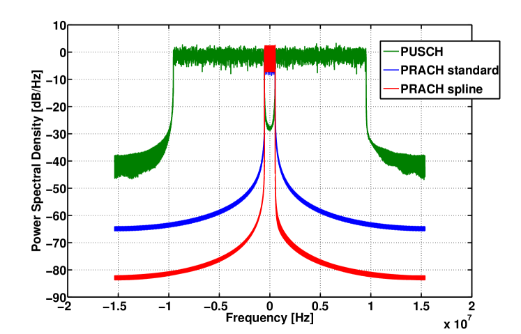
Figure 12: Power spectral density. The power of the PRACH is chosen to achieve a similar PSD as PUSCH.

V-B Data transmission in PRACH

Naturally, using the guard bands for data transmission causes an increased interference level in PUSCH. In Figure 13, we show the effect on PUSCH symbol error rate caused by data transmission on a variable number of D-PRACH subcarriers, given the standard LTE PRACH and the new BFDM-based PRACH approach.

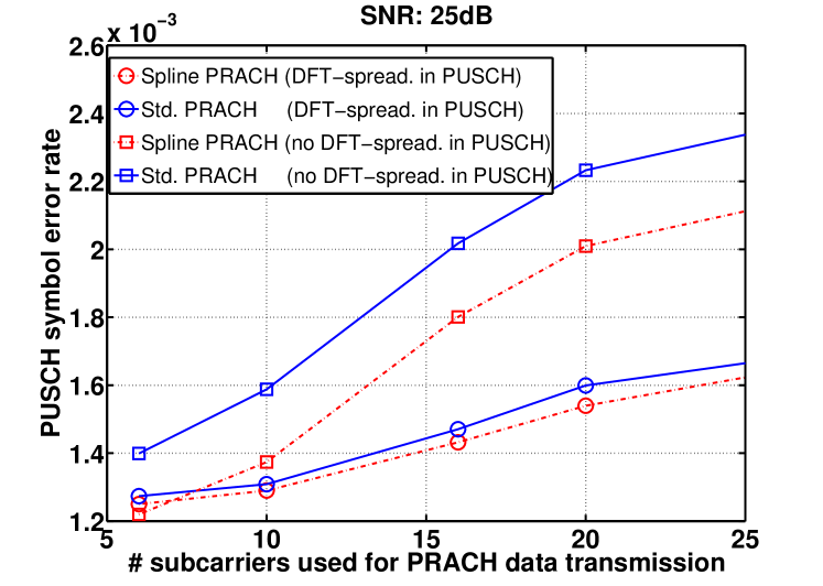
Figure 13: Symbol error rate in PUSCH (averaged over all (1200) subcarriers) plotted over the number of D-PRACH subcarriers. The BFDM-based approach slightly reduces the symbol error rate. This effect is stronger when no DFT spreading is performed in PUSCH.

Clearly, the performance of PUSCH does not deteriorate due to the proposed BFDM-based PRACH. By contrast, irrespective of the actual number of subcarriers used for data transmission, the BFDM-based approach leads to a slightly reduced interference level in PUSCH. Due to the strong influence of the D-PRACH on neighboring subcarriers in PUSCH, this effect is stronger when no DFT-spreading is used in PUSCH. The reason why larger gains, which could be expected from Figure 12, cannot be realized is the PUSCH receiver procedure, which cuts out individual OFDM symbols from the received data.

V-C Asynchronous users

Asynchronous data transmission is a major challenge that comes with MTC and the IoT. Therefore, we now consider a second, completely asynchronous, user that transmits data in the PRACH. Thereby we assign half of the subcarriers available for PRACH data transmission to this second user. However, we still evaluate only the performance of the original “user of interest” (and consequently we carry out channel estimation and decoding only for this user), which is assumed to transmit at the “inner” subcarriers close to the control PRACH. Thereby, we compare two waveforms, OFDM and the proposed spline approach. Figure 14 shows the results.

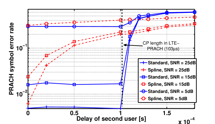
Figure 14: Symbol error rate in PRACH (using 4-QAM) averaged over 10 out of 20 data subcarriers vs. the time offset of a second user. The other subcarriers are used by the second (asynchronous) user. The black line shows the CP length in LTE PRACH.

We observe that for completely asynchronous users, i.e., offsets larger than the CP (in which case OFDM loses its orthogonality property), the new pulse shaped approach reduced the symbol error rate up to a factor of almost one half. Nevertheless, the resulting symbol error rate may still seem excessive. However, as Figure 15 shows, this effect can be compensated by allowing small guard bands (GB) in between the users. Figure 15 compares the performance of no GB and GBs of up to 4 subcarriers, which already drastically reduces the symbol error rate. Interestingly, the spline-based approach without GB achieves roughly the same performance as OFDM with a GB of 4 subcarriers. In other words, we can save 4 subcarriers using the spline-based PRACH.

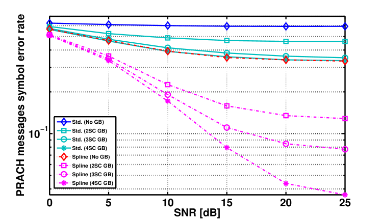
Figure 15: Symbol error rate in PRACH (using 4-QAM) over SNR with presence of a second asynchronous user. Here, the second user has a time offset of $200\,\mu s$. The spline based approach outperforms OFDM with or without a small number of guard bands.

Although the symbol error rates depicted in Figure 14 and Figure 15 may appear excessive, it should be noted that the delays considered in this evaluations (partially exceeding the cyclic prefix length) are unusually high. Figure 16 gives a different picture, focusing on (positive and negative) delays around zero.

V-D Simultaneous time and frequency offsets

Figure 16 illustrates the advantages of the spline-based transmission scheme for both frequency offsets and time delays. We plot the PRACH symbol error rates over the time offset of a second, asynchronous user. In addition, a constant small frequency offset of 62,5 Hz is applied. The SNR is fixed at $25\,\mathrm{dB}$. Moreover, in Figure 16 we assume perfect channel knowledge for the user of interest. It can be observed that the additional frequency offset has a detrimental effect on both schemes, however, the performance loss of OFDM is significantly higher.

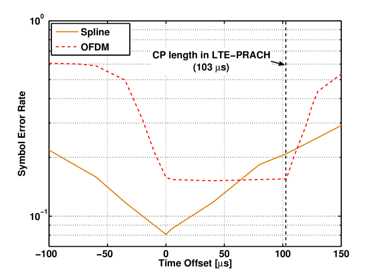
Figure 16: Symbol error rate in PRACH (using 4QAM) with perfect channel knowledge, averaged over 10 out of 20 data subcarriers vs. a varying time offset of a second user with a frequency offset of 62,5 Hz. The SNR is set to $25\,\mathrm{dB}$. The black line shows the CP length in LTE PRACH.

VI Conclusions

We proposed and evaluated a novel pulse shaped random access scheme based on BFDM, which is especially suited in random access scenarios due to very long symbol lengths. It turns out, that the proposed approach is well suited to support data transmission within a 5G PRACH. In particular, numerical results indicate that the BFDM-based approach does not deteriorate PUSCH operations, in fact, it even leads to a slightly reduced interference in PUSCH when using (previously unused) guard bands for data transmission, irrespective of the number of subcarriers used for data transmission. Even more importantly, completely asynchronous users, with time offsets larger than the CP duration in standard PRACH, can be far better supported using the BFDM based approach than using standard OFDM/SCFDMA. The presented results will help to cope with the upcoming challenges of 5G wireless networks and the IoT, such as sporadic traffic.

References

- [1] M. Kasparick, G. Wunder, P. Jung, D. Maryopi, “Bi-Orthogonal Waveforms for 5G Random Access with Short Message Support,” in European Wireless Conference (EW’14). Barcelona, Spain: IEEE Xplore, May 2014.
- [2] G. Wunder, P. Jung, M. Kasparick, T. Wild, F. Schaich, Y. Chen, S. ten Brink, I. Gaspar, N. Michailow, A. Festag, L. Mendes, N. Cassiau, D. Ktenas, M. Dryjanski, S. Pietrzyk, B. Eged, P. Vago, and F. Wiedmann, “5GNOW: Non-Orthogonal, Asynchronous Waveforms for Future Mobile Applications,” IEEE Communications Magazine, vol. 52, no. 2, pp. 97–105, 2014.
- [3] Alcatel-Lucent, Ericsson, Huawei, Neul, NSN, Sony, TU Dresden, u-blox, Verizon Wireless, Vodafone, White Paper.
- [4] F. Schaich, T. Wild, Y. Chen, “Waveform Contenders for 5G - Suitability for Short Packet and Low Latency Transmissions,” in IEEE 79th Vehicular Technology Conference (VTC2014-Spring). Seoul, Korea: IEEE Xplore, May 2014.
- [5] V. Berg, JB. Dor , and D. Noguet, “A multiuser FBMC Receiver Implementation for Asynchronous Frequency Division Multiple Access,” in EuroMicro DSD2014. Verona, Italy: IEEE Xplore, August 2014.
- [6] G. Wunder, P. Jung, and C. Wang, “Compressive Random Access for Post-LTE Systems,” in IEEE ICC Workshop on Massive Uncoordinated Access Protocols, Sydney, Australia, 2014.
- [7] Ji, Yalei and Stefanovic, Cedomir, and Bockelmann, Carsten and Dekorsy, Armin, and Popovski, Petar, “Characterization of Coded Random Access with Compressive Sensing based Multiuser Detection,” in www.arxiv.com/1404.2119, 2014.
- [8] W. Kozek and A. Molisch, “Nonorthogonal pulseshapes for multicarrier communications in doubly dispersive channels,” IEEE Journal Sel. Areas in Commun., vol. 16, no. 8, pp. 1579–1589, 1998.
- [9] S. Sesia, I. Toufik, and M. Baker, LTE, The UMTS Long Term Evolution: From Theory to Practice. Wiley Publishing, 2009.
- [10] F. Schaich and T. Wild, “Relaxed Synchronization Support of Universal Filtered Multi-Carrier including Autonomous Timing Advance,” in ISWCS Workshop on Advanced Multi-Carrier Techniques for Next Generation Commercial and Professional Mobile Systems, Barcelona, Spain, August 2014.
- [11] P. A. Bello, “Characterization of randomly time–variant linear channels,” Trans. on Communications, vol. 11, no. 4, pp. 360–393, 1963.
- [12] P. Jung and G. Wunder, “The WSSUS Pulse Design Problem in Multicarrier Transmission,” IEEE Trans. on Communications, 2007.
- [13] P. Jung, “Pulse Shaping, Localization and the Approximate Eigenstructure of LTV Channels,” The 2008 IEEE Wireless Communications and Networking Conference (WCNC), Las Vegas, USA, Invited Paper, pp. 1114–1119, 2008. [Online]. Available: http://arxiv.org/abs/0912.2828 http://ieeexplore.ieee.org/search/srchabstract.jsp?tp=&arnumber=4489232
- [14] ——, “Weyl–Heisenberg Representations in Communication Theory,” Ph.D. dissertation, Technical University Berlin, 2007. [Online]. Available: http://opus.kobv.de/tuberlin/volltexte/2007/1619
- [15] P. Jung and G. Wunder, “On Time-Variant Distortions in Multicarrier with Application to Frequency Offsets and Phase Noise,” IEEE Trans. on Communications, vol. 53, no. 9, pp. 1561–1570, Sep. 2005. [Online]. Available: http://ieeexplore.ieee.org/xpls/abs_all.jsp?arnumber=1287432
- [16] A. Ron and Z. Shen, “Weyl–Heisenberg frames and Riesz bases in L_2(R^d),” Duke Math. J., vol. 89, no. 2, pp. 237–282, 1997.
- [17] I. Daubechies, “Ten Lectures on Wavelets,” Philadelphia, PA: SIAM, 1992.
- [18] V. D. Prete, “Estimates, decay properties, and computation of the dual function for Gabor frames,” Journal of Fourier Analysis and Applications, 1999.
- [19] R. S. Laugesen, “Gabor dual spline windows,” Applied and Computational Harmonic Analysis, vol. 27, no. 2, pp. 180–194, Sep. 2009.
- [20] O. Christensen, H. O. Kim, and R. Y. Kim, “Gabor windows supported on [-1,1] and dual windows with small support,” Advances in Computational Mathematics, vol. 36, no. 4, pp. 525–545, 2012.
- [21] P. Sondergaard, “Efficient Algorithms for the Discrete Gabor Transform with a Long FIR Window,” Journal of Fourier Analysis and Applications, vol. 18, no. 3, pp. 456–470, 2012.
- [22] L. Vangelista and N. Laurenti, “Efficient implementations and alternative architectures for OFDM-OQAM systems,” IEEE Transactions on Communications, vol. 49, no. 4, pp. 664–675, 2001.
- [23] D. Chu, “Polyphase codes with good periodic correlation properties (corresp.),” IEEE Transactions on Information Theory, vol. 18, no. 4, pp. 531–532, 1972.
- [24] H. Bölcskei, “Blind estimation of symbol timing and carrier frequency offset in wireless OFDM systems,” IEEE Transactions on Communications, vol. 49, no. 6, pp. 988–999, 2001.