Non-linear Plasma Wake Growth of Electron Holes

Abstract

An object’s wake in a plasma with small Debye length that drifts across the magnetic field is subject to electrostatic electron instabilities. Such situations include, for example, the moon in the solar wind wake and probes in magnetized laboratory plasmas. The instability drive mechanism can equivalently be considered drift down the potential-energy gradient or drift up the density-gradient. The gradients arise because the plasma wake has a region of depressed density and electrostatic potential into which ions are attracted along the field. The non-linear consequences of the instability are analysed in this paper. At physical ratios of electron to ion mass, neither linear nor quasilinear treatment can explain the observation of large-amplitude perturbations that disrupt the ion streams well before they become ion-ion unstable. We show here, however, that electron holes, once formed, continue to grow, driven by the drift mechanism, and if they remain in the wake may reach a maximum non-linearly stable size, beyond which their uncontrolled growth disrupts the ions. The hole growth calculations provide a quantitative prediction of hole profile and size evolution. Hole growth appears to explain the observations of recent particle-in-cell simulations.

1 Introduction

The wake behind an object in a plasma that drifts perpendicular to the applied magnetic field is filled in by plasma flow along the field from either side. This flow produces a characteristic multidimensional potential well structure in the wake that attracts ions and repels electrons. The approximate steady-state form of supersonic wake potentials of separated ion streams has been established through one-dimensional models for decades[1, 2, 3] and more recent work has established the subsonic solution requiring multiple dimensions[4, 5]. However, there remains a great deal of uncertainty about the stability of the wake to unsteady short wavelength electrostatic perturbations. The solar-wind wake of the moon[6, 7, 8, 9] is a classic naturally-occuring example of this wake problem, and in-situ satellite measurements have observed various electrostatic fluctuations in it[10, 11]. Several large-scale computational simulations[12, 13, 14, 15] have also shown wake instabilities, but their nature has been controversial. The purpose of the present work is to provide a detailed explanation of the mechanisms that drive the wake instabilities. These may have important applications also for magnetized laboratory plasmas and their interactions with probes.

The idealized configuration we study is represented by a magnetized plasma flowing perpendicular to the field but normal to a flat, thin, object[16]. This is equivalent to a plasma flowing with a sufficiently high Mach number past a spherical (or similar approximately unity aspect ratio) object. The high cross-field velocity in this second case, causes the object to be thin relative to the characteristic lengths in the wake. In other words, the sphere is strongly compressed in the flow direction, when measured in appropriately scaled units. The analysis represents the plasma velocity distribution function in one dimension, along the assumed uniform magnetic field. The plasma is presumed to drift in the transverse, wake direction, with simply a uniform drift velocity. So there is a one to one correspondence between downstream position and time since passing the object’s position. The Debye length is much smaller than the object.

A self-consistent wake potential develops that attracts ions and repells electrons illustrated in Fig. 1.

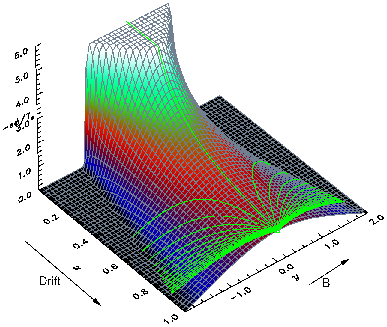
Figure 1: Potential energy structure of electrons as a function of ($x$) distance down the wake and ($y$) position along the magnetic field. (Potential is cut off for viewing purposes at height 5). Example collisionless orbits that arrive at a position on the wake axis are shown. Those that have low parallel energy at the final postion are substantially de-energized. Artificial electron/ion mass ratio of $1/20$ is used to assist the visualization.

In a previous paper[16] it has been shown by integration along orbits that the collisionless electron distribution in the wake potential structure acquires a depression that is localized in velocity. We here call this localized reduction of $f_{e}(v)$ the “dimple”. It is generated on electron orbits that are near the threshold of being reflected by the potential energy hill. These orbits climb the hill, converting their parallel kinetic energy into potential energy. Then, because they approach the peak with very small parallel velocity (they are nearly or just reflected) they spend a long time near the ridge of the potential, and during that time their transverse drift carries them down the potential ridge. Eventually their parallel motion carries them down off the ridge, but not before they have substantially reduced their total energy compared with when they climbed it. They have experienced “drift de-energization”. By contrast electron orbits that are far from the threshold of reflection, having either much more or much less total energy than the potential ridge, spend much less time on the potential ridge. They are far less de-energized. The distribution function is constant along orbits in a collisionless plasma. So if the external distribution is monotonically decreasing in kinetic energy (e.g. a Maxwellian) then an orbit that started (outside the potential structure) at a higher total energy (because of de-energization) has a phase-space density $f(v)$ lower than orbits that have experienced less de-energization. This is the qualitative explanation of the mechanism forming the dimple. Its form was calculated quantitatively by numerical orbit integration in reference [16].

The distribution function dimple that arises is linearly unstable to Langmuir waves. Therefore one expects this de-energization effect to excite electrostatic instabilities, which will have a tendency to fill in and smooth out the distribution non-linearly until the growth rate is suppressed. Because the dimple size depends strongly on the electron to ion mass ratio, the free energy available prior to non-linear saturation (which was calculated) also depends on mass ratio; simulations that use artificially low mass ratio are therefore liable to obtain unphysically large fluctuation levels. For true mass ratios the energy available to instabilities is only $10^{-4}$ to $10^{-3}$ of the electron thermal kinetic energy; so the level of Langmuir wave turbulence expected is modest.

The purpose of the present work is to pursue further the non-linear development of the instability driven by this de-energization mechanism so as to explain what is observed in recent large-scale simulations of this problem[17]. Those simulations clearly observe the formation of the electron distribution dimple, but the observations are of course of its self-consistent non-linear state.

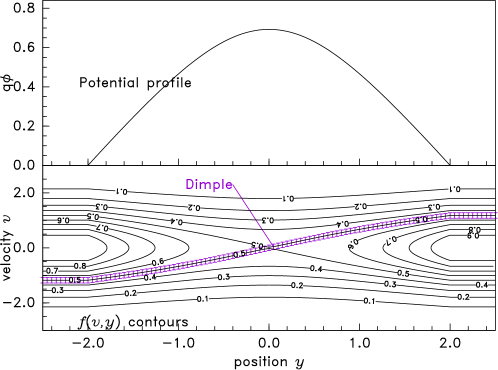
Figure 2: Illustrative electron phase-space orbits in the vicinity of the wake’s potential energy hill. The hill extends along the parallel $y$ coordinate to the edge of the wake. The dimple lies along the lower left to upper right branches of the separatrix, hatched.

In phase space (see Fig. 2), the dimple is centered along the separatrix contour of constant total energy that the wake potential defines. In addition to incoherent noise, we observe small persistent coherent structures, like eddies, localized to the dimple in phase space. They propagate in along the dimple with approximately the local electron velocity (and acceleration). These structures, which (we will show) are electron holes, therefore leave the simulation, moving to large parallel distance, quite quickly. The exception to this behavior is that holes move much more slowly near the x-point of the energy contours (where the phase-space velocity is zero) which is naturally at the ridge of the wake potential structure. As the simulations progress (down the wake) eventually one (or more) of the electron holes near the x-point grows to a large size, and disruption of the ion velocity distribution occurs. There is a large amount of free energy in the ion distribution, because the ions are in two streams, of modest energy spread, with opposite velocities ($>c_{s}$). The strong hole growth and disruption of these streams occurs at a place where (time when) linearized calculation indicates that the ion streams are stable because of their large separation. The puzzle that our current analysis addresses is how the perturbation becomes large enough to disrupt the ion streams well before they themselves become linearly unstable. Our answer is that the mechanism is a non-linear one involving electron holes.

In section 2 we formulate the Boltzmann equation for the parallel electron distribution, and solve it approximately analytically in a potential of specified shape to find the electron dimple at the potential ridge. This solution supplements the prior numerical orbit integrations[16] by providing an analytic form for the dimple, in particular its velocity-width. In view of the substantial approximations required to achieve this analytic solution, section 3 approaches the problem instead, by an integration in the parallel direction rather than along the two-dimensional orbits. This alternative (and equivalent) formulation shows that the drift (de-energization) effects can be conceptualized as a term in the one-dimensional Boltzmann equation of approximately the “Krook” collision form. Solving this equation gives an identical expression for the dimple, through a conceptually different set of approximations.

The second formulation is more useful for incorporating the effects of presumed quasilinear diffusion filling in the dimple. Section 4 explains the expected consequences of a self-consistent level of incoherent turbulence. It is shown that this system cannot explain the growth of perturbations to sufficient amplitude to disrupt the ions and tap into their energy until a place on the wake is reached where the ion streams are very close to linear instability. In other words, it cannot explain what is observed in the simulations.

Section 5 provides an explanation and analysis of the coherent electron holes, and shows that the drift de-energization mechanism can be equivalently regarded as the drift convection of holes into regions of higher background density. This effect causes holes to grow in depth and velocity width. The self-consistent growth of hole width with background density and the resulting hole profile (for quasi-neutral holes) is calculated analytically for Maxwellian background electrons and beam ions. Holes that retain their integrity and remain near the ridge of the wake potential structure (the x-point) can grow to sizes sufficient to disrupt the ion streams when the density increase is of the order of one e-folding. Moreover their characteristics are consistent with what is observed in the simulations. Therefore we interpret the pre-linear-threshold disruption of the ion streams as caused by the long-term non-linear growth of electron holes until they become energetic enough to tap the ion free energy.

2 Solving For the Dimple in Two Dimensions

2.1 Boltzmann’s Equation with drift and quasilinear diffusion

Including ad hoc quasilinear velocity-space diffusion[18] with coefficient $D$, we can write Boltzmann’s equation as

$$\left({\partial\over\partial t}+{\bf v}.\nabla+{\bf a}.\nabla_{v}\right)f=\nabla_{v}(D\nabla_{v}f).$$ (1)

which for the one-dimensional distribution, magnetized case with coordinate $y$ in the magnetic field direction, and $x$ in the perpendicular direction becomes

$${d\over dt}f=\left({\partial\over\partial t}+v{\partial\over\partial y}-{q\over m}{\partial\phi\over\partial y}{\partial\over\partial v}\right)f=-v_{x}{\partial f\over\partial x}+{\partial\over\partial v}\left(D{\partial f\over\partial v}\right).$$ (2)

Here the right hand side can be considered the additional source terms in the 1-D Boltzmann equation arising respectively from drift de-energization and quasilinear velocity space diffusion. We will consider a time-independent situation: ${\partial\over\partial t}=0$ and constant drift $v_{x}$. Velocity $v$ written without a subscript refers here to $v_{y}$, the parallel velocity, and the distribution function is one-dimensional along $y$.

The orbits are the characteristics of the left-hand side. They are the paths in (parallel) phase space corresponding to constant energy

$${\cal E}={1\over 2}mv^{2}+q\phi=const.$$ (3)

They are most easily found as the contours of constant energy in phase space.

2.2 Collisionless Orbits in Specified Potential

We take parameters to be normalized so that velocities are in units of the cold ion sound speed $c_{s}=\sqrt{T_{e}/m_{i}}$, and potential is in units $T_{e}/e$. The perpendicular distance is scaled such that $x=$distance$/M_{\perp}$ where $M_{\perp}=v_{x}/c_{s}$. Then the normalized energy equation for electrons becomes ${\cal E}={1\over 2}m_{r}v^{2}-\phi$, where $m_{r}\equiv m_{e}/m_{i}$.

The dimensionless potential form is considered to be controlled by dynamics separate from what happens to the instabilities. The specific form illustrated in Fig. 1 is based on an approximate solution in the form of two expansions of plasma into a vacuum, patched at the symmetry axis as discussed previously[16]. However, the only features of this potential shape that substantially matter in the present context are that $-\phi$ is symmetric and single-peaked in $y$, having a known curvature near the ridge at $y=0$ and being zero beyond a certain $y$-distance; and that it decays from a large value at $x\sim 0$ monotonically in the perpendicular. i.e. downstream wake ($x$) direction. So we will simply specify that

$\bullet$ $\phi_{0}(x)$ is the monotonic potential at $y=0$;

$\bullet$ the curvature is given in terms of a scale length $w$ by ${\partial^{2}\phi\over\partial y^{2}}=-\phi_{0}/w^{2}(x)$;

$\bullet$ and $y=Y(x)$ is the edge of the perturbed potential.

[A model potential that fits simulation results with $T_{i}=T_{e}$ has $\phi_{0}=-1/1.2x$, $Y=1+2x$, and $w=(1+2x)/1.66$.]

Now since in normalized units

$$v={1\over c_{s}}{dy\over dt}={dy\over dx},$$ (4)

the equation of the electron orbits in 2-D space may be written in the vicinity of the ridge, in terms of an expansion as

$$m_{r}{d^{2}y\over dx^{2}}={\partial\phi\over\partial y}=-{\phi_{0}\over w^{2}}y$$ (5)

Because of the smallness of $m_{r}$ the orbits do not have a large duration ($x$-extent). So it makes sense to approximate ${\phi_{0}/w^{2}}$ as a constant, ignoring its $x$-dependence. Then the orbit can be solved trivially as

$$y={v_{0}\over k}\sinh(k[x-x_{0}])$$ (6)

where

$$k^{2}=-\phi_{0}/m_{r}w^{2}$$ (7)

and $x_{0}$ and $v_{0}$ are the position and velocity of the orbit when $y=0$. The approximations leading to this expression are not well justified near the edge of the perturbed region (and not at all outside it), nevertheless most of the orbit of electrons that cross the ridge slowly is spent near the ridge. It is therefore reasonable to use eq. (6) to estimate the orbit duration $X=x_{0}-x$ (considered the duration either in time or in space, since $x$ and $t$ are interchangable) from the edge of the perturbed region to $y=0$. It can then be considered the solution of

$$\sinh(kX)=kY/|v_{0}|.$$ (8)

In order for the approximations adopted to be consistent, both sides of this equation must be large compared with unity. Therefore $\sinh\approx{1\over 2}\exp$ and

$$kX\approx\ln\left[2kY\over|v_{0}|\right]=\ln\left[2\sqrt{|\phi_{0}|}\,Y\over\sqrt{m_{r}}w|v_{0}|\right].$$ (9)

2.3 Resulting Distribution Without Diffusion

The electron distribution function at $y=0$, when $D=0$, can be deduced by considering the change in total parallel energy ${\cal E}$ arising from the perpendicular drift term. To the extent that $y\ll x$ applies to the relevant parts of the orbit (which we’ve already assumed to be a good approximation), the potential energy change arising from cross-field drift (which is the drift de-energization) can be estimated from the $x$-gradient of the potential at the ridge

$$\delta{\cal E}=-\int{\partial\phi\over\partial x}{dx\over dt}dt\approx-\int_{x}^{x_{0}}{d\phi_{0}\over dx}dx=\phi_{0}(x_{0}-X)-\phi_{0}(x_{0})\approx-{d\phi_{0}\over dx}X$$ (10)

(to first order in $X/x_{0}$). Substituting for $X$ we get

$$\delta{\cal E}\approx-{d\phi_{0}\over kdx}\ln(2kY/|v_{0}|)=-{d\phi_{0}\over dx}{\sqrt{m_{r}}w\over\sqrt{|\phi_{0}|}}\ln\left(2\sqrt{|\phi_{0}|}\,Y\over\sqrt{m_{r}}w|v_{0}|\right).$$ (11)

This energy is not included in the parallel energy conservation along the orbit. In other words, denoting the kinetic energy at the start of the orbit by ${\cal K}_{\infty}={1\over 2}m_{r}v_{\infty}^{2}$, and when it reaches the ridge ${\cal K}_{0}={1\over 2}m_{r}v_{0}^{2}$, we have

$${\cal K}_{\infty}={\cal K}_{0}-\phi_{0}+\delta{\cal E}.$$ (12)

Consequently at $x=x_{0}$, $y=0$, the distribution function $f_{0}$ is different from the (presumed) Maxwellian at the orbit start:

$$f_{0}/{n_{\infty}\over\sqrt{2\pi T}}=\exp(-{\cal K}_{\infty})=\exp(\phi_{0}-{\cal K}_{0}-\delta{\cal E})\\ \approx\exp(\phi_{0})\exp(-{1\over 2}m_{r}v_{0}^{2})\left[\sqrt{m_{r}}w|v_{0}|\over 2\sqrt{|\phi_{0}|}Y\right]^{P},$$ (13)

where

$$P={d\phi_{0}\over kdx}={d\phi_{0}\over dx}{w\over\sqrt{|\phi_{0}|}}\sqrt{m_{r}}$$ (14)

At the characteristic distance down the wake $x_{0}\sim 1$, all quantities $\phi_{0}$, $d\phi_{0}/dx$, $w$, and $Y$ are of order unity. So $P$ is of order the square root of the mass ratio $\sqrt{m_{r}}$.

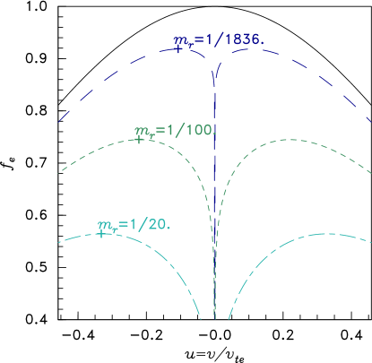
Figure 3: The dimple in the electron distribution at $y=0$, $f_{0}$ as a function of normalized electron velocity $u$, for three different electron to ion mass ratios $m_{r}$. The cross marks the dimple width, where $f_{0}^{\prime}=0$. The parameters are $\phi_{0}=-1.32$, $d\phi_{0}/dx=0.96$, $w=1.15$ (so $P=0.96\sqrt{m_{r}}$), and $Y=2$.

The dimple in the electron velocity distribution function is illustrated in Fig. 3, in which electron velocity has been expressed normalized to its thermal velocity $u=v_{e}/\sqrt{2T_{e}/m_{e}}=v_{0}\sqrt{m_{r}/2}$. The dimple arises in this Vlasov case as a final multiplication factor on the otherwise Maxwell-Boltzmann behavior. It actually dominates the behavior near $v_{0}=0$ forming a cusp. Strictly speaking our approximations are quantitatively unjustified as $u\to 0$, but the qualitative observation that a cusp forms is correct. The approximations also assume $m_{r}v_{0}^{2}(=2u^{2})\ll 1$ and so the factor in brackets is small. But the power $P$ to which the factor is raised is also small. The derivative of $f_{0}$ with respect to $v_{0}$ from this expression can readily be shown to be zero where

$$u^{2}={1\over 2}m_{r}v_{0}^{2}={1\over 2}P$$ (15)

which is a small quantity, of order the square root of the electron/ion mass ratio, $m_{r}$. This condition may also be written

$$v_{0}=\left(-{d\phi_{0}\over dx}{w\over\sqrt{|\phi_{0}|}}\right)^{1/2}{1\over m_{r}^{1/4}},$$ (16)

which indicates the approximate width of the dimple in velocity space. This width is dictated by the electron/ion mass ratio. Therefore simulations that use artificially increased mass ratio ($m_{r}=m_{e}/m_{i}\gg 1/1836$) will increasingly misrepresent the electron behavior.

3 Solving for $f$ by Parallel Integration

Thus far we have approached the problem accounting fully for two space dimensions and discussing integration along orbits in 2-D space plus 1-D velocity. Solving the problem analytically has required major approximations, but has given a reasonable estimate of the result when there is no velocity-space diffusion.

A different approach to solving for the dimple is to do integration not along the 2-D spatial orbits but along only 1-D ($y$) in space. That is actually how eq. (2) is organized. 2-D orbit integration takes the first term on the RHS to be part of the orbit characteristics (and so far has not included the second diffusive term). By contrast 1-D integration of the equation leaves the $v_{x}$-convective term on the RHS, and integrates along a fixed $x$ path in which $y$ and $v$ vary. This is then a truly 1-D (but phase-space) treatment, but instead of $f$ being constant on orbits, it varies in accordance with the terms remaining on the RHS.

Within this perspective, we can regard the two terms on the RHS as being dimple-generating convective de-energization, and quasilinear diffusion. To some degree they will balance one another: one tending to form the dimple, the other to smooth it away. The solution for $f$ at some position $y$ can be found in principle by starting in the unperturbed background region $y_{Y}$ (actually at $y=Y$, the edge of the potential perturbation), and integrating orbits inward to position $y$. In principle the solution is simply

$$f(y,v_{y})-f(y_{Y},v_{Y})=\int-v_{x}{\partial f\over\partial x}+{\partial\over\partial v}\left(D{\partial f\over\partial v}\right)dt.$$ (17)

This integration must be taken along phase-space orbits of constant ${\cal E}={1\over 2}mv^{2}+q\phi(y)$, and in practice needs to be done in terms of position.

$$f(y,v_{y})-f(y_{Y},v_{Y})=\int_{y_{Y}}^{y}-v_{x}{\partial f\over\partial x}+{\partial\over\partial v}\left(D{\partial f\over\partial v}\right){dy\over v}.$$ (18)

This integral determines the difference between the actual $f$ and the Maxwell-Boltzmann approximation (a Maxwellian scaled by $\exp(\phi)$).

A solution by this technique requires us to know what the value of the terms in the RHS integral are. Focussing first on the convective de-energization term $v_{x}\partial f/\partial x$, we don’t know its value exactly until we have the solution everywhere. However, it may in some circumstances be reasonable to approximate it in a manner which avoids us having to solve the full-scale integro-differential system. One such approximation is to presume that the shape of the dimple changes only slowly with $x$-position. If so, then the dominant contribution to $\partial f/\partial x$ can be estimated to be the variation of the overall level of $f$, which is approximately the Maxwell-Boltzmann. Its variation with $x$ (in normalized parameters) is $f\propto\exp(\phi)$, in which case

$${v_{x}\over f}{\partial f\over\partial x}=-v_{x}{\partial\phi\over\partial x}\equiv-\nu_{x}.$$ (19)

Here $\nu_{x}$ is like a collision frequency. And indeed, the term in the Boltzmann equation to which this approximation corresponds is a “Krook” collisional term $-\nu_{x}f$. Since the orbits of interest spend most of their time near the potential ridge at $y=0$, it is reasonable to take $\nu_{x}$ to be uniform, given by taking $\phi=\phi_{0}$. That is the main approximation of this treatment.

Incorporating just this term (i.e. taking $D=0$) for now, we can perform the integral along constant-$x$ based upon the resulting equation

$${1\over f}\left(v{\partial\over\partial y}-{1\over m_{r}}{\partial\phi\over\partial y}{\partial\over\partial v}\right)f={1\over f}{df\over dt}=-\nu_{x},$$ (20)

whose solution is

$$f(y,v_{y})/f(y_{Y},v_{Y})=\exp[-\nu_{x}(t-t_{Y})]$$ (21)

Thus the deviation from Maxwell-Boltzmann distribution can be considered to be an exponential multiplicative factor whose argument is proportional to the time an orbit takes to reach the position $y$.

Notice that the dimensionless form for $d/dt$ in eq. (20) shows the terms on the LHS are usually very large compared with the convective de-energization term (the $\nu_{x}$ term). That term is important only where the LHS terms are nearly zero, i.e. near $y=0$ where ${\partial\phi\over\partial y}=0$ and at values of $v$ nearly equal to zero. In other words, the dimple generation takes place predominantly at the axis, for velocities near zero there. However, it is not that the contribution to $df/dt$ is larger there, it is that the orbit spends far more time there than anywhere else. Passing that region in phase space contributes most strongly to $t-t_{Y}$.

The duration, $X=t-t_{Y}$, of the orbit to the position $y=0$ has already been solved for in section 2.2. It was there taken as an approximation that variation of $\partial\phi/\partial y$ with $x$ could be ignored. Here it is no approximation, because we are integrating along $x=$constant. Instead the approximation has been made in $df/dx$. In any case, we can immediately appropriate the solution eqs. (8) and (9) as

$$X\approx{1\over k}\ln\left[2kY\over|v_{0}|\right]=\sqrt{m_{r}\over\phi_{0}}w\ln\left[2\sqrt{|\phi_{0}|}\,Y\over\sqrt{m_{r}}w|v_{0}|\right].$$ (22)

It should be no surprise that substituting this result into eq. (21) gives exactly the same dimple as previously: eq. (13).

What we’ve demonstrated, therefore, is that the dimple formation can be calculated by explicit integration at fixed $x$, based upon an approximation of the drift de-energization term in a Krook form. This demonstration gives some additional confidence in the prior treatment. But it also gives us a more direct way to incorporate quasilinear diffusion, and (later) to understand electron hole growth.

4 Quasilinear Electron Velocity Diffusion

Now we consider the effects of instabilities that will arise as the dimple forms and prevent it from ever becoming the deep cusp that the Vlasov treatment finds. One possible result of such instabilities, if they consist of many incoherent modes, is an effective quasilinear velocity-space diffusion. That’s the case we discuss first.

4.1 Self-consistent Diffusion level

Under this assumption, the physics of the steady state is that the diffusion magnitude, $D$, adjusts itself corresponding to a moderate time-independent level of turbulence sufficient to maintain the distribution function at an approximately neutral stability. It is reasonable (if the Debye length is small compared to other lengths in the problem) to assume that the growth rate of the electron instabilities is intrinsically large compared with other timescales in the problem. In that case, $D$ must adjust itself so that the instability threshold is never significantly exceeded. In other words, marginal stability is always approximately satisfied.

Solving for the distribution function in those circumstances requires us to suppose that as we integrate along the orbit we encounter levels of quasilinear diffusion that are just sufficient to maintain the distribution function marginally stable. Doing so requires that in phase-space regions where the RHS terms are important (i.e. mostly near $y=0$ and $v=0$) the diffusion term counterbalances the convective de-energization term.

When the two RHS terms exactly balance

$$-\nu_{x}f+{\partial\over\partial v}\left(D{\partial f\over\partial v}\right)=0.$$ (23)

When $D$ is (approximately) independent of $v$, and $f$ deviates only a small amount from constant, i.e. in the vicinity of a shallow dimple, the solution is of this equation is a parabola. However, we don’t require that the terms exactly balance for orbits whose duration is sufficiently short that the perturbation introduced by $\nu_{x}$ is small. The dimple can therefore be considered to be constrained to have a positive second derivative (equal to $\nu_{x}/D$) over a region around $v=0$ that extends to a speed ($|v|$) at which $\nu_{x}X$ becomes smaller than of order unity. Outside that velocity region, the second derivative of $f$ can become negative, as it must in order to merge the dimple with the bulk of the electron distribution function. The details of that outer region depend on how quickly the constraint eq. (23) is relaxed, whether $D$ varies with $v$ and so on. Such details cannot be precisely calculated using the analytic principles on which this treatment is based. Some ansatz must be adopted. A simple and plausible one is to choose to represent the dimple as a negative Gaussian perturbation to the bulk Maxwellian distribution. The velocity width of the dimple Gaussian, expressed as $2v_{d}$ such that the Gaussian is $\propto\exp(-v^{2}/v_{d}^{2}$), is determined by $\nu_{x}X\sim 1$.

The plasma fluctuation level adjusts the diffusion coefficient $D$ to achieve marginal stability. If $D$ is small, the dimple is deep, because its magnitude is such as to give second derivative $\nu_{x}/D$ near its peak. If $D$ is large the dimple is shallow. Thus, orbit duration determines the width, and marginal stability determines the depth of the dimple. The dimple width is given (see eq. 16) by $v_{d}\sim v_{0}\sim m_{r}^{-1/4}$ (in units of $c_{s}$) or $u_{d}\sim\sqrt{2}\;m_{r}^{1/4}$ (in units of $v_{te}$).

4.2 Electron Marginal Stability

The dispersion relation of electrostatic waves is $\epsilon=1+\chi=0$. Instability requires the real part of the susceptibility $\chi_{r}$ to be negative at frequency $\omega$ in the upper half of the complex plane where the imaginary part of $\chi$ is zero. A bulk Maxwellian electron distribution (ignoring ions for now), contributes a susceptibility real-part approximately $\Re(\chi_{e})=1/k^{2}\lambda_{De}^{2}$ (at wave phase velocities small compared with the electron thermal speed). The contribution from a dimple Gaussian of temperature $T_{d}$ and negative density $-n_{d}$ is the same but multiplied by $-n_{d}T_{e}/n_{e}T_{d}$. So the total (real part) electron susceptibility is

$$\Re(\chi_{e})={1\over k^{2}\lambda_{De}^{2}}\left[1-{n_{d}\over n_{e}}{T_{e}\over T_{d}}\right].$$ (25)

Because $k$ is essentially a free choice, it can be adjusted for any negative value of $\Re(\chi_{e})$ to make $\Re(\chi_{e})=-1$. For a symmetric distribution such as we are considering, the imaginary part of the susceptibility, $\Im(\chi_{i})$, is zero at $\omega=0$; so negative $\Re(\chi_{e})$ is sufficient (as well as necessary) for instability. Marginal stability of electrons alone is therefore at $n_{d}T_{e}/n_{e}T_{d}=1$, which means

$${n_{d}\over n_{e}}={T_{d}\over T_{e}}\sim m_{r}^{1/2}.$$ (26)

However, if we just focus on the zero-velocity peak,

$${f_{d}(0)\over f_{e}(0)}={n_{d}\over n_{e}}\left(T_{e}\over T_{d}\right)^{1/2}=\left(T_{d}\over T_{e}\right)^{1/2}\sim m_{r}^{1/4}.$$ (27)

The dimple depth at marginal stability should be a quite noticeable decrease in the distribution function at zero velocity, fractionally $1/1836^{1/4}\sim 1/7$. Fig. 4 illustrates some cases. Comparison with Fig. 3 shows that these depths, if anything, somewhat overestimate what is expected from filling in the collisionless dimple by diffusion.

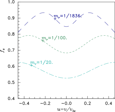
Figure 4: Electron distributions representing a dimple of negative Maxwellian form with temperature equal to $m_{r}^{1/2}T_{e}$ that are marginally stable with immobile ions.

A crude upper bound on the magnitude of the potential perturbation that will produce quasilinear diffusion sufficient to maintain marginal stability can be estimated as follows. Quasilinear diffusion presumes the cumulative effect of stochastic orbits produced by multiple modes of different phase velocities. How many modes are involved is uncertain, but what is certain is that it is at least greater than one, and that therefore the amplitude of any one unstable mode is insufficient of itself to flatten the distribution (at marginal stability). A mode whose phase-space island size is equal to the width of the dimple ($\sim 2v_{d}$) is large enough on its own to flatten the distribution. The single-mode perturbation sufficient to create such an island width is (in normalized units) $\tilde{\phi}\sim m_{r}^{1/2}$ and is the upper bound of the perturbed potential at quasi-linear marginal stability. This potential makes a very small perturbation to the ions, a fractional energy perturbation of only $m_{r}^{1/2}/v_{i}<m_{r}^{1/2}\sim 1/50$.

More generally, quasilinear velocity-space diffusivity of particles by a resonant spectrum of waves of specified electric field (or potential) is proportional to the inverse square of the particle mass. The ion streams’ velocities place them inside the dimple, subject to the same resonant spectrum of waves as the electrons. They will experience a diffusivity smaller by a factor $m_{r}^{2}=1836^{-2}$. Negligible ion perturbation occurs at electron marginal quasilinear turbulence levels. The free energy of the ions cannot be tapped by quasilinear electron instabilities.

4.3 Ion susceptibility contribution

When the ions have effectively a two-stream distribution in the region under consideration, they contribute further to instability by negative contribution to the real part of the susceptibility. The contribution for low-temperature equal-density beams of velocity $\pm v_{i}$ (in units of $c_{s}$) is

$$\Re(\chi_{i})\approx-{1\over k^{2}\lambda_{De}^{2}}{1\over v_{i}^{2}}.$$ (28)

This is sufficient to make a system with purely Maxwellian electrons unstable when $v_{i}\leq 1$, which is the upper edge of the ion-ion instability region in a “Stringer” plot[19]. If the ion speed is not a great deal higher than this threshold, then the ion contribution modifies the electron marginal stability condition, rendering it:

$${n_{d}\over n_{e}}={T_{d}\over T_{e}}(1-1/v_{i}^{2})\sim m_{r}^{1/2}(1-1/v_{i}^{2}).$$ (29)

The marginal-stability depth of the dimple is somewhat decreased. And to make the dimple shallower in the presence of constant $\nu_{x}$, the magnitude of of the quasilinear diffusion coefficient, $D$, must be larger by the factor $v_{i}^{2}/(v_{i}^{2}-1)$.

Nevertheless, when $v_{i}$ (the ion mach number) substantially exceeds 1 (the upper limit for ion-ion instability), the ion susceptibility contribution does not change the linear marginal stability condition by very much. It does not much enhance the required quasilinear diffusivity nor the level of turbulence required to produce it, and it does not substantially raise the typical phase-space island width of the incoherent modes at which quasilinear stabilization occurs.

Ion instability drive does not change the conclusion that incoherent quasilinear flattening of the electron dimple would occur at fluctuation levels that are too low to make significant non-linear modification to the ion distribution. The linear drive of the combined electron and ion distributions is brought to zero, if the ion velocities are significantly higher than the ion-ion stability threshold $c_{s}$, well before the quasilinear diffusivity of the ions is significant, and before entrainment of the ions into typical mode sizes. This conclusion is consistent with the code observation[17] of a sustained initial period when the ion distribution evolution is quiescent and laminar, and the electron fluctuations are predominantly localized to their phase-space separatrix. But it fails to explain the coherent structures that are observed to grow and entrain the ions even well before the ion beam velocities have slowed into the unstable regime.

5 Electron Holes

5.1 Hole Structural Relationships

At the other end of the spectrum of treatments of non-linear effects and turbulence, far from the quasilinear diffusion approach, lies the phenomenon of phase-space “holes”. Conventionally such a hole[20, 21, 22, 23, 24, 25, 26] refers to a localized coherent perturbation of the distribution function phase-space density that is self-binding via its self-consistent potential. A perturbation to a one-dimensional electron distribution function $f_{e}(y,v)$ can be self-binding if it traps electrons. To do so it must give rise to an electric potential that is positive in the hole. That requires the perturbation of the phase-space density, denoted $\tilde{f}_{e}$ to be negative: a deficit of electrons. (Likewise ion holes require a negative $\tilde{f}_{i}$.) The parallel spatial coordinate is written $y$, for consistency with previous sections. Velocities $v$ are unnormalized in this section.

Electron holes in one dimension can exist at spatial scales from less than the Debye length, upward. The hole is essentially a Bernstein-Greene-Kruskal (BGK) mode[27]: a trapping structure that self-consistently satisfies the Vlasov-Poisson system of equations. There is substantial freedom in the form that such modes can take. Entropy arguments[23] support what is more often proposed as an ansatz[28] that the velocity dependence of $f_{e}$ in the trapped region is approximately parabolic (with positive curvature, negative temperature) leading to what is called a Maxwell-Boltzmann hole. They suggest that the most probable spatial extent of a shallow electron hole is approximately 4 times the plasma shielding length. However, the precise shape of the hole proves not to have a major effect on its properties, and modeling the hole as a rectangular box in $y,v$ space, of constant depth, yields parameters that differ little from the Maxwell-Boltzmann hole[23]. It is therefore plausible to approximate the hole’s shape with simple model functions, and still expect to arrive at scalings that have reasonable quantitative validity. Moreover, deep holes with spatial extent much larger than the shielding length are possible.

The self-consistent Poisson’s equation for an electron hole in one dimension of space may be written

$$\left(-{\partial^{2}\over\partial y^{2}}+{1\over\lambda^{2}}\right)\phi={\rho\over\epsilon_{0}}$$ (30)

where $\lambda$ is the plasma shielding length, and $\rho$ is the charge-density of the hole. The shielding length would normally be thought of as the Debye length $\lambda_{De}=\sqrt{\epsilon_{0}T_{e}/ne^{2}}$ but it can be generalized to account for ion shielding and for arbitrary distribution functions by regarding it as arising from the medium’s polarization term which is responsible for the dielectric susceptibility[23]. The real part of the linearized susceptibility for wave number $k$ and phase velocity $\omega/k=v_{p}$ is then

$$\Re(\chi)={1\over k^{2}\lambda^{2}}=\sum_{species}{\omega_{p}^{2}\over k^{2}}{\cal P}\int{df_{b}\over dv}{dv\over v_{p}-v},$$ (31)

and this is the definition of $\lambda$. $f_{b}$ denotes the unperturbed background distribution away from the hole; ${\cal P}$ denotes the principal value of the integral, and contributions like this from both electrons and ions are included.

We consider a localized peaked hole potential structure that is the solution of Poisson’s equation (30). The potential energy then has a well, which Fig. 5 illustrates schematically.

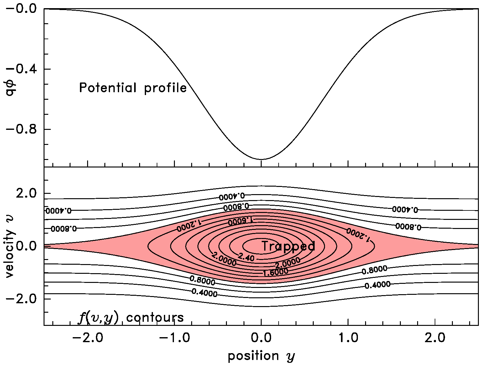
Figure 5: Contours of constant $f$ are contours of constant total energy in phase space. An attractive potential produces an island, which can become a hole. The parallel spatial extent of $y$ here should be considered far less than the width of the wake shown in Fig. 2.

For simplicity, and because it is the important case here, we take the hole to be stationary (corresponding to $v_{p}=0$), though moving structures can naturally be treated by a change of reference frame. It gives rise to phase-space orbits of electrons (along which $f_{e}$ is constant) that are the contours of constant kinetic plus potential energy, so they satisfy

$${1\over 2}m_{e}v^{2}+q\phi=const.={1\over 2}m_{e}v_{b}^{2}$$ (32)

where we write $q$ for the electron charge (it is negative), and $v_{b}$ is the velocity at a distant unperturbed (“background”) position ($y_{b}$) far from the hole, where the potential is $\phi=0$ (so this potential is measured relative to the background plasma potential in the vicinity of the hole). Since the potential energy $q\phi$ is negative, orbits that connect to $y_{b}$ have a minimum speed at any position given by

$$v_{s}(y)=\sqrt{-2q\phi(y)\over m_{e}},$$ (33)

which is the boundary of the trapped-electron island in phase space. The charge density to be used in eq. (30) is then

$$\rho(y)=q\int\tilde{f}(y,v)dv,$$ (34)

where $\tilde{f}$ is the change of $f$. It is zero ($\tilde{f}=f(y,v)-f(y_{b},v_{b})=0$, $|v|>v_{s}$) on untrapped orbits , while on trapped orbits $|v|<v_{s}$,

$$\tilde{f}(y,v)=f(y,v)-f(y,v_{s})=f(y,v)-f(y_{b},0).$$ (35)

See Fig. 6.

Figure 6: Schematic illustration of the distribution function $f(v)$ in an electron hole. The reference distribution is uniform within the trapped region ($|v|<v_{s}$) and the difference $\tilde{f}$ is what determines the binding charge density.

The total electron density in the presence of the potential perturbation would be different at position $y$ from its value at $y_{b}$ even if $\tilde{f}$ were everywhere zero, because $\int f(y,v)dv\neq\int f(y_{b},v)dv$. However, in Poisson’s equation (30), that difference is contained in the $\phi/\lambda^{2}$ term, not in $\rho$. It is the linearized dielectric response of the plasma. In eq. (30) the $\rho$ contains only the charge density attributable directly to $\tilde{f}$.

Now we introduce a lumped-parameter model of the hole in which $\tilde{f}$ has a characteristic magnitude at the center of the hole $\tilde{f}_{0}=\tilde{f}(0,0)$, and the characteristic widths in velocity, $v$, and space, $y$, of the trapped region are $\Delta v$ and $\Delta y$ respectively. We define $\Delta v$ so that the charge density at the hole’s spatial center ($y=0$) is

$$\rho=\rho(0)=q\tilde{f}_{0}\Delta v.$$ (36)

In Poisson’s equation the term $\partial^{2}\phi/\partial y^{2}$ will be of magnitude approximately $\phi(0)/\Delta y^{2}$. But if the hole has large spatial extent, $\Delta y\gg\lambda$, that term is negligible and we find as a quasi-neutral approximation to the hole

$${\phi\over\lambda^{2}}\approx{\rho\over\epsilon_{0}}={q\over\epsilon_{0}}\tilde{f}_{0}\Delta v.$$ (37)

(The quasi-neutral hole can be considered to be two “double-layers” that trap electrons between them. A small hole that is not quasi-neutral can be analysed[23, 22] to find a comparable relationship between $\phi$ and $\Delta v$, in which the proportionality coefficient depends upon $\Delta y/\lambda$. So our conclusions are not qualitatively changed for holes of small $\Delta y$.)

Hereafter, we refer to values at $y=0$ and we drop the repetition of this fact in our notation. There is a proportionality between the two measures of the hole velocity width $v_{s}$ and $\Delta v$. It requires knowledge of the velocity-shape of the hole to obtain its exact coefficient. For example, if $\tilde{f}$ is uniform throughout the trapped region, then $\Delta v=2v_{s}$ while if $\tilde{f}$ is parabolic in the trapped region, then $\Delta v={4\over 3}v_{s}$, and if it is triangular $\Delta v=v_{s}$. Adopting this last alternative, for reasons that will become clear later, we have

$$\Delta v=v_{s}=\sqrt{-2q\phi\over m_{e}},$$ (38)

and the relationship between the depth and velocity-width of the hole becomes

$$-\tilde{f}={\epsilon_{0}m_{e}\Delta v\over 2q^{2}\lambda^{2}}={n_{b}\Delta v\over 2\omega_{pe}^{2}\lambda^{2}}=\left(\lambda_{De}\over\lambda\right)^{2}{n_{b}\Delta v\over v_{te}^{2}}={\sqrt{\pi}}\left(\lambda_{De}\over\lambda\right)^{2}f_{b}(0){\Delta v\over v_{te}}.$$ (39)

where $v_{te}\equiv\sqrt{2T_{e}/m_{e}}$ and parameters such as $\lambda_{De}$, $\omega_{pe}$, $f_{b}$ and $n_{b}$ refer to the background plasma. Different assumptions about hole profile shape will somewhat change the coefficient. But in general, when the shielding length is not too different from the Debye length, the fractional hole depth $\tilde{f}/f_{b}$ is roughly equal to the fractional velocity-width $\Delta v/v_{te}$ for a quasi-neutral ($\Delta y\gg\lambda$) hole.

Since $f$ cannot be negative there is a maximum hole depth and size obtained by setting the trapped distribution function (phase-space density) equal to zero i.e. $-\tilde{f}=f_{b}(0)$. Then

$${\Delta v\over v_{te}}={1\over\sqrt{\pi}}\left(\lambda\over\lambda_{De}\right)^{2}.$$ (40)

5.2 Hole Growth

In view of the proportionality between the hole depth $|\tilde{f}|$ and its velocity-width $v_{s}$, for a hole to grow in velocity width (and hence in potential) it must become deeper. When this happens in an effectively collisionless plasma, the shape of the hole, $\tilde{f}(v)$, is determined not by maximizing entropy but by the constancy of $f$ on orbits. The absolute value of $f$ on trapped orbits ($f_{t}$) is an invariant function[20] of the orbit’s action ($\int vdx$), provided the hole phase-space orbits remain closed. (Fine-scale mixing does not substantially change the mean $f$ on a phase-space orbit, and so does not escape this constraint. In recognizing it we abandon decisively the common presumption that the hole remains parabolic.) Therefore the only way for a hole to become deeper is that the external distribution function $f(y,v_{s})=f(y_{b},0)$ increases. In Dupree’s analysis[29] of growth of moving ($v_{p}\not=0$) holes in an electron-ion instability, the way the external $f$ increases is by the hole decelerating to lower $|v_{p}|$ so that $f(y_{b},v_{p})$ increases (e.g. for a Maxwellian external distribution). In the present context, however, there is a different mechanism inducing hole growth. It is that the plasma is drifting in the $x$ direction, perpendicular to the magnetic field. Consequently there is a convective time derivative of the external density: $v_{x}{\partial f\over\partial x}$; and this is indeed positive in the wake. In other words, the drift de-energization term in the Vlasov equation that has the effect of generating the dimple continues to operate if a hole is present, and is a cause of hole-growth. Or equivalently, perhaps conceptually simpler still, the hole experiences a background plasma of rising density because of drift. The importance of these remarks is that the growth of a hole is not suppressed quasilinearly by reaching sufficiently strong perturbation that the distribution function is flattened. The hole is coherent; and as long as that coherence is maintained, it continues to grow as $f(y_{b},0)$ grows.

The only way a hole stops growing short of maximal size, assuming there is insufficient turbulence to tear it apart, is for it to convect out of the spatial region where the external $f$ is growing. Holes move mostly along the direction of the (unperturbed) phase space orbits. Therefore their parallel ($y$-) motion leaves them at approximately constant $f$. When a hole moves away from the peak of the wake’s potential profile, it is therefore swept out of the wake, at approximately the electron parallel velocity, without any consequent growth. Once the hole reaches the unperturbed plasma outside the wake, no convective growth term is operating, and it will move away without further growth.

Therefore, once a hole has formed with sufficient coherent integrity, the only condition for it to grow is that it stays inside the wake, which in general means it must remain near the peak of the wake’s potential energy curve (bottom of its electrostatic potential well) $y=0$. That hole position is unstable, so most holes will move from it, and then be convected out of the wake before they’ve grown large, because the electron orbit duration in the $x$-direction is rather small except when they are on axis. But a few may remain at the wake axis long enough to grow to near maximal size. It is those we now analyse.

There is a linear relationship between $\tilde{f}$ and $v_{s}$ if $\lambda$ and the hole shape can be approximated as constant. Since the growing edge of a hole entrains additional phase-space area on which the distribution is equal to $f_{b}(0)$, the hole velocity profile in this approximation is triangular. That was the basis for choosing the triangular profile in the previous section. But we now do a self-consistent calculation that shows what the shape in velocity space of a growing quasi-neutral hole profile actually is. This requires a treatment that is self-consistent and, for a deep hole, non-linear (i.e. avoiding the commonly used linearized plasma response explained in the prior section). It is most simply performed for a quasi-neutral hole by setting the net charge density to zero as follows.

Consider a background plasma with Maxwellian electrons,

$$f_{b}(v)={n_{b}\over v_{te}\sqrt{\pi}}\exp(-u^{2}),$$ (41)

where $v_{te}\equiv 2T_{e}/m_{e}$ and $u\equiv v/v_{te}$. Write the normalized phase-space separatrix speed $u_{s}$ at potential $\phi$: $u_{s}^{2}=-q\phi/T_{e}$. This is positive because $\phi$ is positive and $q$ negative for electrons. Take the reference flat-top electron distribution to be constant within the trapped region, and constant along untrapped orbits as shown in Fig. 6:

$$f_{f}(v)={n_{b}\over v_{te}\sqrt{\pi}}\times\left\{\begin{array}[]{ll}\exp(u_{s}^{2}-u^{2})&\mbox{for $u\geq u_{s}$}\\ 1&\mbox{for $u<u_{s}$}\\ \end{array}\right..$$ (42)

This is the distribution that would arise if an electron-trapping potential hill arose slowly (compared with the electron bounce time) in a background distribution that was not varying with time. The density of this distribution is a function of the normalized potential, $u_{s}^{2}$. It can readily be evaluated[20] as

$$n_{f}(u_{s}^{2})=\int f_{f}dv=n_{b}\left[{2u_{s}\over\sqrt{\pi}}+{\rm e}^{u_{s}^{2}}{\rm erfc}(u_{s})\right].$$ (43)

The ions in the wake can be represented quite well[2, 17] by two ion streams, each of narrow spread in speed. Near the wake axis they are equal and opposite. We take their Mach number outside the hole to be $M=v_{b}/c_{s}$. Inside the hole the ion speeds are lower, because the hole repels ions, and by conservation of energy the mach number there is $\sqrt{M^{2}-2u_{s}^{2}}$. Hence, by conservation of flux, the ion density is

$$n_{i}(u_{s}^{2})=n_{b}{M\over\sqrt{M^{2}-2u_{s}^{2}}}$$ (44)

If the actual electron distribution in the trapped region is $f_{t}(v)$, different from the reference $f_{f}$ by $\tilde{f}$, then quasi-neutrality can be expressed as the cancellation of the charge arising from the background density in the perturbed potential, $n_{f}-n_{i}$, and the hole charge density $\propto\int_{0}^{u_{s}}\tilde{f}du$. That is,

$$n_{f}-n_{i}=n_{b}H(u_{s})/\sqrt{\pi}=v_{te}f_{b}H(u_{s})=2v_{te}\int_{0}^{u_{s}}f_{b}-f_{t}\;du,$$ (45)

where in the trapped-region $f_{f}=f_{b}$ is independent of $u$; $f_{b}$ refers to the background value $f_{b}(0)$ at $u=0$; and the function $H$, for any given $M$, is essentially the normalized reference charge-density from both electron and ion distributions,

$$H(u_{s})=\sqrt{\pi}\left[{2u_{s}\over\sqrt{\pi}}+{\rm e}^{u_{s}^{2}}{\rm erfc}(u_{s})-{M\over\sqrt{M^{2}-2u_{s}^{2}}}\right],$$ (46)

which must be cancelled by the hole charge-density.

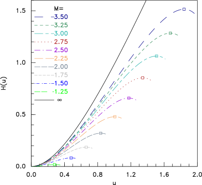
Figure 7: The charge-density function $H(u)$ for various values of ion mach number $M$. The solid line marked $\infty$ corresponds to an immobile ion background density independent of potential.

Figure 7 shows the form of $H(u)$.

Equation (45) determines the relationship between the hole velocity-width, $u_{s}$, and the changing background electron density expressed as the peak of its Maxwellian, $f_{b}$. In the context of a growing hole, the actual trapped electron distribution $f_{t}$ remains invariant once formed. Therefore we can differentiate the equation with respect to the hole width, $u_{s}$, and it becomes

$${d\over du_{s}}[H(u_{s})f_{b}]=2u_{s}{d\over du_{s}}f_{b}.$$ (47)

No contribution arises to the differential from the fixed $f_{t}(u)$, and none comes from the limit because $f_{b}=f_{t}$ at $u=u_{s}$: the newly trapped electrons have phase-space density equal to the instantaneous background density. This equation can be written as a simple quadrature

$$\int{df\over f}=\int{dH\over 2u-H}.$$ (48)

The derivative $H^{\prime}(u)=dH/du$ is positive at moderate $u$, but reaches zero at a certain value $u=u_{max}$ dependent on $M$. This is where the hole reaches its maximum possible size. At that size the rate of hole width-increase with respect to background density becomes infinite: the hole blows up. Its growth can no longer be described by the quasi-neutral hole equilibrium equations. We call the corresponding value of the background distribution $f_{b}=f_{max}$. And we find a set (at various $M$) of universal curves by numerical integration from $u_{max}$ backwards toward zero. So that

$$\ln(f/f_{max})=\int_{u_{max}}^{u}{H^{\prime}\over 2u-H}du.$$ (49)

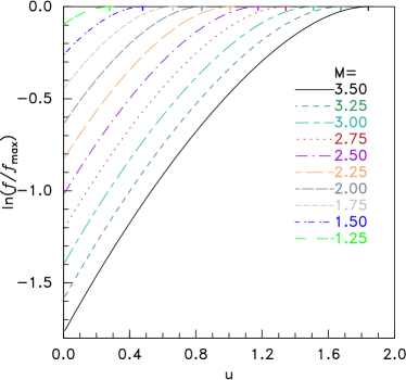
Figure 8: Trapped electron distribution function forms for various ion Mach numbers. These also give the hole growth curves arising in growing background density.

Fig. 8 shows the result. The significance of a curve for some given $M$ is this. As a hole moves from one value of $f$ to a larger value, the hole size, $u_{s}$, grows by moving along the curve. As it does so, the trapped distribution function is built up within the hole by incrementally trapping additional phase-space. The shape of $f_{t}(u)$ is therefore also given precisely by this functional dependence. So these curves can be considered to represent the shape in velocity space ($u$) of a hole that grows from infinitesimal size up to any finite current size $u_{s}$. The boundary of the hole is $u_{s}$, at which $f_{t}=f_{b}$, and inside the hole $f_{t}(u)=f_{b}\exp[\ln(f(u)/f_{max})-\ln(f_{b}/f_{max})]$. If the hole started at finite size $u_{init}$, with a trapped distribution inside $u_{init}$ different from the growing hole form, nothing changes except in the initial region of the hole $u\leq u_{init}$. It must begin from a trapped distribution that satisfies the quasi-neutrality equation (45) but its initial shape will be determined by whatever mechanisms governed its formation. Thereafter, as it grows incrementally, driven by rising external density, it follows the curve, and the trapped distribution function is built up accordingly.

No hole can grow stably beyond $u_{max}$, the place where the curves’ gradient becomes zero. That size is the maximum stable hole size. When it is reached, the hole blows up, and disruption of the ion streams will take place: their large free energy will be released through additional non-linear processes not described here. It is found that an excellent fit to the numerical values of $u_{max}$ for the range of $M$ shown is

$$u_{max}=M/\sqrt{2}-0.6.$$ (50)

A hole that begins at a position with a certain value of $f_{b}$ or equivalently background density $n_{b}$, will grow as $n_{b}$ grows, provided it remains near the wake potential ridge, not convecting out of the wake. It will reach the disruptive size when the density has increased by a factor that can be read off the curves of Fig. 8. For example, the $M=2.5$ curve has $\ln(f/f_{max})=-1$ at $u=0$, so a small hole will reach disruptive size when the density has increased by a factor $\exp(1)$. Or again for $M=2$, $\ln(f/f_{max})=-0.5$ at $u=0.1$, so a hole that starts with size $u_{s}=0.1$ will grow to disruption when $n/n_{init}=\exp(0.5)$.

The wake axis experiences a large increase of background density ($n_{b}=n_{\infty}\exp(e\phi/T_{e})$) as its potential subsides from the large negative values immediately behind the object. It is clear, therefore, that holes formed in this region that remain at the axis have sufficient density increase to reach disruptive size. This conclusion contrasts with the demonstration that quasilinear diffusion cannot reach a level of strong ion perturbation.

These analytic conclusions are in accord with the observations in the simulations. Small electron holes form in the dimple (by mechanisms we don’t here calculate in detail). While they remain near the axis and are not convected out of the wake, they grow. Some eventually grow large enough to disrupt the ion streams.

6 Summary

The wake behind an object in a magnetized plasma with predominantly cross-field drift, and short Debye length, experiences one-dimensional electrostatic instabilities. The electron velocity distribution along the field acquires a depression we call the dimple, on orbits that spend a long time near the axial ridge of the potential energy structure of the wake. The driving term of this unstable dimple can equivalently be regarded as either de-energization of the electrons by drift perpendicular to $B$, down the potential energy ridge; or, as drift in an increasing background density, filled in by parallel velocity less quickly for orbits with low parallel velocity near the ridge. The term may be approximated in the “Krook” collisional form in Boltzmann’s equation.

The second viewpoint, of drift into increasing background density, provides a more transparent understanding of the resulting non-linear dynamics. The collisionless form of the dimple is immediately unstable to electrostatic waves near the wake axis, having phase velocities lying within the dimple velocity width of approximately $(m_{e}/m_{i})^{-1/4}c_{s}=(m_{e}/m_{i})^{1/4}v_{te}/\sqrt{2}$ (approximately $7c_{s}$ for hydrogen plasmas). The waves will grow and, if incoherent, will fill in the electron distribution function dimple until it becomes marginally stable. The ion parallel velocity distribution consists of two streams attracted inward toward the wake axis. They contain a great deal of free energy. But, because the stream velocity spacing is large close to the object, the ion distribution is not itself linearly unstable until far downstream. Nevertheless, it is observed in numerical simulations (and sometimes in space) that large-amplitude perturbations grow and substantially disrupt the ion streams, long before they have become linearly unstable.

The electric fields associated with quasilinear velocity-space diffusivity sufficient to stabilize the electron distribution dimple are too small to cause substantial perturbation of the ions. The ion disruption therefore cannot be explained by linear or quasilinear instability growth. However, the driving term of electron instability is effective also in causing the non-linear growth of electron holes. Holes formed away from the wake axis, or that move away from it, leave the wake at approximately the electron phase-space separatrix orbital speed before they can grow very much. Some holes, however, are formed at the wake axis and remain near it. When they do, the continuing background density enhancement causes them to grow to a maximum size beyond which they explode and disrupt the ion streams. We have calculated the form, the growth, and the maximum size of such electron holes, establishing a (to our knowledge) new theoretical non-linear instability mechanism associated with cross-field drift into higher density regions. Electron holes grown by this mechanism provide the missing piece of the wake stability puzzle. Coherent hole growth is not suppressed quasilinearly, and explains how large, ion-disrupting, perturbations can occur before the ion streams become themselves linearly unstable.

Undoubtedly, there are many other important phenomena in the moon wake, including Alfvénic processes that the present electrostatic treatment omits. But, because of their large linear growth rate, we consider the electrostatic instabilities to be primary. Several important details of the explanation remain to be investigated. We have not addressed the question of exactly how small electron holes form in the first place, nor have we quantitatively analysed their positional stability, which decides whether or not they remain at the wake axis and grow. Moreover, the present treatment, limited to parallel one-dimensional dynamics, omits oblique wave-vector perturbations, which might in some circumstances be important. Nevertheless, the qualitative agreement with phenomena observed in one-dimensional simulations provide strong evidence that the electron hole growth mechanism is the key explanation of these simulations at least.

References

- [1] Y C Whang. Interaction of the magnetized solar wind with the Moon. Physics of Fluids, 11:969–975, 1968.
- [2] A V Gurevich, L P Pitaevskii, and V V Smirnova. Ionospheric aerodynamics. Space Science Reviews, 9:805–871, 1969.
- [3] A V Gurevich and L P Pitaevsky. Non-linear dynamics of a rarefied ionized gas. Progress in Aerospace Sciences, 16(3):227–272, 1975.
- [4] I H Hutchinson. Oblique ion collection in the drift approximation: How magnetized Mach probes really work. Physics of Plasmas, 15(12):123503, 2008.
- [5] I H Hutchinson and L Patacchini. Flowing plasmas and absorbing objects: analytic and numerical solutions culminating 80 years of ion-collection theory. Plasma Physics and Controlled Fusion, 52(12):124005, December 2010.
- [6] J M Bosqued, N Lormant, H Reme, and C D’Uston. Moon‐solar wind interactions: First results from the WIND/3DP Experiment. Geophysical Research Letters, 23(10):1259–1262, 1996.
- [7] K W Ogilvie, J T Steinberg, R J Fitzenreiter, C J Owen, A J Lazarus, W M Farrell, and R B Torbert. Observations of the lunar plasma wake from the WIND spacecraft on December 27, 1994. Geophysical Research Letters, 23(10):1255–1258, 1996.
- [8] J. S. Halekas, S D Bale, D L Mitchell, and R P Lin. Electrons and magnetic fields in the lunar plasma wake. Journal of Geophysical Research, 110(A7):A07222, 2005.
- [9] J S Halekas, V Angelopoulos, D G Sibeck, K K Khurana, C T Russell, G T Delory, W M Farrell, J P McFadden, J W Bonnell, D Larson, R E Ergun, F Plaschke, and K H Glassmeier. First Results from ARTEMIS, a New Two-Spacecraft Lunar Mission: Counter-Streaming Plasma Populations in the Lunar Wake. Space Science Reviews, 165(1-4):93–107, January 2011.
- [10] Paul J Kellogg, Keith Goetz, Steven J Monson, J Bougeret, Robert Manning, and M L Kaiser. Observations of plasma waves during traversal of the moon’s wake. Geophysical Research Letters, 23(10):1267–1270, 1996.
- [11] J. B. Tao, R. E. Ergun, D. L. Newman, J. S. Halekas, L. Andersson, V. Angelopoulos, J. W. Bonnell, J. P. McFadden, C. M. Cully, H.-U. Auster, K.-H. Glassmeier, D. E. Larson, W. Baumjohann, and M. V. Goldman. Kinetic instabilities in the lunar wake: ARTEMIS observations. Journal of Geophysical Research, 117(A3):1–10, March 2012.
- [12] W M Farrell, M L Kaiser, J T Steinberg, and S D Bale. A simple simulation of a plasma void: Applications to Wind observations of the lunar wake. Journal of Geophysical Research, 103(10):23,653–23,660, 1998.
- [13] Paul C. Birch and Sandra C. Chapman. Detailed structure and dynamics in particle-in-cell simulations of the lunar wake. Physics of Plasmas, 8(10):4551, 2001.
- [14] E. Kallio. Formation of the lunar wake in quasi-neutral hybrid model. Geophysical Research Letters, 32(6):1–5, 2005.
- [15] Shinya Kimura and Tomoko Nakagawa. Electromagnetic full particle simulation of the electric field structure around the moon and the lunar wake. Earth, Planets and Space, 60(6):591–599, July 2008.
- [16] I. H. Hutchinson. Electron velocity distribution instability in magnetized plasma wakes and artificial electron mass. Journal of Geophysical Research, 117(A3):1–11, March 2012.
- [17] C B Haakonsen, I H Hutchinson, and C Zhou. Kinetic electron and ion instability of the lunar wake simulated at physical mass ratios. submitted to Physics of Plasmas, 2015.
- [18] Ronald C Davidson. Methods in Nonlinear Plasma Theory. Academic Press, New York, 1972.
- [19] T. E. Stringer. Electrostatic instabilities in current-carrying and counterstreaming plasmas. Journal of Nuclear Energy. Part C, Plasma Physics, 6:267–279, 1964.
- [20] A V Gurevich. Distribution of captured particles in a potential well in the absence of collisions. Sov. Phys. JETP, 26:575–580, 1968.
- [21] H L Berk, C E Nielsen, and K V Roberts. Phase Space Hydrodynamics of Equivalent Nonlinear Systems: Experimental and Computational Observations. Physics of Fluids, 13(4):980, 1970.
- [22] Hans Schamel. Electron holes, ion holes and double layers. Physics Reports, 140(3):161–191, July 1986.
- [23] Thomas H. Dupree. Theory of phase-space density holes. Physics of Fluids, 25(2):277, 1982.
- [24] V Maslov and H Schamel. Growing electron holes in drifting plasmas. Physics Letters A, 178:2–5, 1993.
- [25] M V Goldman, D L Newman, and R E Ergun. Phase-space holes due to electron and ion beams accelerated by a current-driven potential ramp. Nonlinear Processes in Geophysics, 10:37–44, 2003.
- [26] B. Eliasson and P.K. Shukla. Formation and dynamics of coherent structures involving phase-space vortices in plasmas. Physics Reports, 422(6):225–290, January 2006.
- [27] I B Bernstein, J M Greene, and M D Kruskal. Exact nonlinear plasma oscillations. Physical Review, 108(4):546–550, 1957.
- [28] H Schamel. Theory of Electron Holes. Physica Scripta, 20(3-4):336–342, September 1979.
- [29] T. H. Dupree. Growth of phase-space density holes. Physics of Fluids, 26(9):2460, 1983.