Revealing latent factors of temporal networks for mesoscale intervention in epidemic spread

The customary perspective to reason about epidemic mitigation in temporal networks hinges on the identification of nodes with specific features or network roles. The ensuing individual-based control strategies, however, are difficult to carry out in practice and ignore important correlations between topological and temporal patterns. Here we adopt a mesoscopic perspective and present a principled framework to identify collective features at multiple scales and rank their importance for epidemic spread. We use tensor decomposition techniques to build an additive representation of a temporal network in terms of mesostructures, such as cohesive clusters and temporally-localized mixing patterns. This representation allows to determine the impact of individual mesostructures on epidemic spread and to assess the effect of targeted interventions that remove chosen structures. We illustrate this approach using high-resolution social network data on face-to-face interactions in a school and show that our method affords the design of effective mesoscale interventions.

Keywords: complex networks, temporal networks, tensor decomposition, epidemic spread, high-resolution social networks, human contact networks, targeted interventions

Many natural and artificial systems are adequately represented in terms of interaction networks between their components ¹. The network representations has led to key insights on the relation between the structure of these systems and the dynamics of diverse processes that take place over the network, such as information diffusion, epidemic spread, and much more ^{2; 3}. In recent years, the availability of time-resolved network data has pushed network science beyond the static graph representation and has prompted new research on understanding and modeling time-varying graphs, commonly referred to as temporal networks ⁴. This has spurred an intense activity on studying how dynamical processes are affected by the temporal evolution of the network on which they unfold, focusing on heterogeneous distributions of inter-event times (“burstiness”), heterogeneous activity distributions, causality constraints, etc. ^{5; 6; 7; 8; 9; 10; 11; 12; 13; 14; 15; 16}. High-resolution social network data ^{17; 18; 19; 20}, in particular, have opened the way to richer individual-based models of epidemic spread ^{18; 21; 22; 23} and have raised new questions on designing control strategies for epidemic processes in temporal networks ^{22; 24; 25; 26}. However, micro-interventions that operate on individual nodes, such as targeted vaccination, are difficult to implement, both for lack of high-resolution data in general cases and because action at the level of individuals is subjected to many informational and operational constraints. Therefore, it is natural to consider interventions that target important collective patterns and structural units of temporal networks. Since network communities, i.e., cohesive clusters, have long been recognized as key structural units in the architecture of complex networks ²⁷, it is natural to think of interventions at the community level ^{28; 23}. Time-varying networks, however, can exhibit a richer range of activity/connectivity patterns than static networks. Defining and detecting temporal network structures at the intermediate (“meso”) scale, as well as understanding their relevance for dynamical processes occurring on the networks, remains a largely open question with important applications. Early work on the mesoscale structure of complex networks has mostly focused on static networks ²⁹ and on community detection in temporal networks ³⁰. Recently, latent factor analysis techniques have been used to simultaneously detect topological and temporal activity patterns of time-varying networks ³¹.

Here we tackle the problem of designing interventions that selectively target the mesoscopic structure of a temporal network, with the goal of controlling a dynamical process such as epidemic spread. This requires both detecting mesostructures and ranking them by their importance for a specific dynamical process. To detect mesostructures we build on the work of Ref. 31 and use tensor decomposition techniques ³² to represent a temporal network as an additive superposition of mesostructures, each of which can encode complex structural and temporal correlations. To assess the importance of individual mesostructures, we take advantage of the additivity of the tensor decomposition, which allows us to dissect the original network and reassemble altered temporal networks where chosen mesostructures are selectively removed. By comparing the dynamics of a given process on the original network and on the altered ones we can then determine the specific role of individual mesostructures and we can rank the effectiveness of interventions that target those structures for removal.

We illustrate our approach using high-resolution social network data on face-to-face interactions in a school setting and investigating the importance of individual mesostructures for simple epidemic processes. Schools are actually an interesting context for models of epidemic spread, as they are thought to play an important role in the community spread of infectious diseases ^{33; 34; 35; 36; 37}. Macro-scale interventions such as school closure are considered a viable strategy for epidemic mitigation ³⁸ but come with steep socio-economic costs ^{39; 40}, thus calling for more targeted approaches. We show that our approach identifies effective strategies for epidemic mitigation that involve the targeted removal of individual mesostructures. Remarkably, we find that the most important mesostructures for epidemic spread correspond neither to the strongest structures nor to cohesive structures that can be easily detected by community detection methods.

Mesoscale structure of temporal networks

Latent factor analysis of temporal networks

We first summarize a general framework that we introduced in ref. 31 to expose the mesoscale structure of a temporal network. The approach combines a tensor representation of a temporal network ⁴¹ and a dimensionality reduction technique based on tensor decomposition ³².

We consider an undirected and unweighted temporal network, hence the state of the network at time $t$ can be represented by a binary-valued adjacency matrix $\textbf{M}(t)\in\mathbb{R}^{N\times N}$, where the matrix entry $M_{ij}(t)$ indicates the status of link $i$-$j$ at time $t$, and $N$ is the number of nodes of the network. The matrices describing the state of the network at different times can be combined into a 3-mode tensor, $\mathcal{T}\in\mathbb{R}^{N\times N\times L}$, where the first two dimensions are the customary node indices of the adjacency matrix and the third dimension is a temporal index. $L$ is the number of network snapshots, each for a different point in time. To detect structures, i.e., correlated activity/connectivity patterns of the temporal network, we set up a latent factor analysis based on non-negative tensor factorization ³¹: The central idea is to approximate the tensor $\mathcal{T}$ with a sum $\tilde{\mathcal{T}}$ of rank-1 non-negative tensors (see Methods):

$$\mathcal{T}\,\simeq\,\tilde{\mathcal{T}}=\sum_{r=1}^{R}\,\mathcal{S}_{r}\ .$$ (1)

with $R<\min{\{N,S\}}$. This decomposition allows to describe the original temporal network as a purely additive superposition of a chosen number of activity/connectivity patterns, encoded by the individual tensor components. Each component $\mathcal{S}_{r}$ is regarded as a mesoscale structure of the temporal network and can encode cohesive clusters (i.e., communities), temporally-localized mixing patterns, and more. Such a parts-based representation is a general and powerful feature of tensor decompositions with non-negativity constraints ⁴² and greatly enhances the interpretability of individual components. A similar approach based on non-negative matrix factorization has been proposed to detect overlapping communities in static networks ⁴³.

The additive decomposition of Eq. 1 also suggests a natural way to investigate the role played by individual mesoscale structures, both on the overall network architecture and on the dynamics of processes occurring over the network, e.g., epidemic spread. In particular, we can assess the importance of individual mesostructures for dynamical processes unfolding over the temporal network by selectively removing those structures: We can start from the decomposition of Eq. 1, remove a chosen term (i.e., a chosen structure), and sum all the other terms, obtaining a modified temporal network where the chosen structure has been selectively erased. We can then simulate a given dynamical process over the original temporal network and over the modified temporal network, and compare the dynamics or the outcome of the process, hence learning about the impact of the removed structure.

Case study

As a case study we consider an empirical temporal network of human face-to-face interactions in a primary school ⁴⁴, measured by using wearable sensors ¹⁹. The dataset describes the interactions (or “contacts”) between $231$ children aged $6$ to $12$ and $10$ teachers, organized in $10$ classes. It comprises the contacts that occurred at the school premises during two consecutive days in October 2009, from 8:30am to 5:15pm of each day. We chose this dataset because it is publicly available ^{44; 23} and provides not only a high-resolution temporal network, but also ground truth information on communities, namely, class attributes for all nodes. Moreover, the school schedule is known and can be used to understand the activity patterns that mix multiple classes, as done in Ref. 31. In the following this will allow us to relate the effect of removing an individual component to specific knowledge about the social behavior associated with that component.

The school data are naturally represented as a temporal network, where nodes are individuals and links are interactions between pairs of nodes. The networks snapshots of our dataset are recorded every $20$ seconds, however the school activity is scheduled on a coarser temporal scale. Hence, we aggregate the data over consecutive time intervals of $15$ minutes to obtain unweighted network snapshots: for every $15$-minute interval, a link is drawn between two nodes if the corresponding individuals had at least one contact during that interval. This yields a temporal network represented by binary-valued valued tensor ${\mathcal{T}}$ with $N=241$ and $L=70$.

Following ref. 31, we carry out the non-negative tensor factorization of Eq. 1 and approximate the tensor $\mathcal{T}$ with the sum $\tilde{\mathcal{T}}$ of $R=14$ components (see Methods and Supplementary Information): the results of the decomposition are reported in Fig. 1. Components $\mathcal{S}_{1}$ through $\mathcal{S}_{9}$ and component $\mathcal{S}_{11}$ correspond to the $10$ school classes of the school. They can be validated using the know class attributes for students and teachers, and they can also be detected to some extent using community detection algorithms on the temporally-aggregated network ³¹. The components $\mathcal{S}_{10}$, $\mathcal{S}_{12}$, $\mathcal{S}_{13}$ and $\mathcal{S}_{14}$, however, mix individuals from different classes and – contrary to the above class components – they are only active during lunch breaks. Such components cannot be found by community detection of the temporally-aggregated networks as they correspond to temporally-localized mixing patterns of the temporal network, due to mixing of students at lunch time. Tensor decomposition, however, can naturally detect these patterns as well as the customary cohesive network communities.

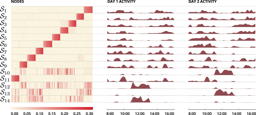
Figure 1: Components obtained by tensor factorization of the school temporal network. Each row is associated with one component $\mathcal{S}_{r}=\mathbf{a_{r}}\,\circ\,\mathbf{a_{r}}\,\circ\,\mathbf{c_{r}}$ of the tensor decomposition $\tilde{\mathcal{T}}$ in Eq. 5 (see Methods), with $R=14$. Components are ordered top to bottom according to their Euclidean norm. Left-hand color-coded matrix: Node weights for each component. Each row corresponds to a vector $\mathbf{a_{r}}$ of the decomposition, normalized to unity in Euclidean norm for clarity of visualization. Nodes are ordered to expose the block structure of the matrix due to school classes. Right-hand plots: Component activity as a function of time over the 2-day span of the dataset. Each row correspond to a vector $\mathbf{c_{r}}$, normalized to unity in Euclidean norm. Components $\mathcal{S}_{1}$ to $\mathcal{S}_{9}$ and component $\mathcal{S}_{11}$ are school classes, while components $\mathcal{S}_{10}$, $\mathcal{S}_{12}$, $\mathcal{S}_{13}$ and $\mathcal{S}_{14}$ mix individuals from different classes and are active during lunch breaks.

We remark that whereas the original temporal network $\mathcal{T}$ is unweighted, the approximating network $\tilde{\mathcal{T}}$ is in general weighted (see Methods). For any given network snapshot, corresponding to a $15$-minute time interval, we will interpret the weight of the edge between two nodes as the cumulated time that those nodes spent in contact over that $15$-minute interval. In Table 1 we report the fraction of total tensor weight corresponding to each of the $R=14$ components, $\|\mathcal{S}_{r}\|\,/\,\|\tilde{\mathcal{T}}\|$.

r	1	2	3	4	5	6	7
weight fraction	11.3%	8.6%	8.8%	7.1%	8.3%	6.9%	5.7%
r	8	9	10	11	12	13	14
weight fraction	6.8%	7.5%	7.5%	4.8%	6.8%	5.7%	6%

Table 1: Component weight. Fraction of total tensor weight corresponding to each term $\mathcal{S}_{r}$ of the decomposition $\tilde{\mathcal{T}}$.

Mesoscale targeted interventions for epidemic spreading

Intervention design and evaluation

The decomposition of a temporal network into a superposition of components, interpreted as mesostructures, makes it possible to pinpoint and assess the contribution of individual mesoscopic features to the overall structural and functional properties of the temporal network. Indeed, the additive decomposition of Eq. 1 allows to selectively remove a chosen component $s$ by excluding the corresponding term, yielding an altered temporal network,

$$\tilde{\mathcal{T}}^{s}=\sum_{r\neq s}\,\mathcal{S}_{r}\ ,$$ (2)

which can be compared to the original network to elucidate the specific role of component $s$. When component $s$ can be interpreted in terms of a specific behavioral pattern (e.g., the lunch breaks of Fig. 1) its removal can be regarded as the effect of an intervention strategy that selectively targets that behavior (e.g., removing lunch breaks from the school schedule).

As a first step in exploring mesoscale interventions, here we focus on the case study of the previous section and investigate the effect of removing individual mesostructures on the dynamics of simple epidemic processes unfolding over the school temporal network. We study how the timing and size of the epidemic are affected by the removal of individual network components, that is, by different targeted interventions aimed at removing them.

We start with the simple case of a susceptible-infected (SI) process. Each network node can be in either of two states: susceptible (S) or infected (I). A susceptible node in contact with an infected one becomes infected with a fixed probability $\lambda$ per unit time. Once infected, a node stays indefinitely in that state. The system is initialized with all nodes in the S state, except for a single infected node (seed node). The timing and duration of contacts between nodes is described by the temporal network $\tilde{\mathcal{T}}$, which is a sequence of weighted networks: for each network snapshot, the weight of an edge between two nodes gives the total duration of the contacts between those nodes during the corresponding time interval. Although the SI process does not describe any realistic infectious disease, it represents a paradigmatic dynamical process and it is frequently used to investigate the structural properties of temporal networks.

To investigate the effect on epidemic spread of removing a chosen mesostructure $\mathcal{S}_{r}$, we simulate the epidemic process on the altered network $\tilde{\mathcal{T}}^{r}$, and compare its dynamics to that observed on the full temporal network $\tilde{\mathcal{T}}$. We quantify the effect of removing component $r$ by measuring the epidemic delay ratio ²⁴

$$\tau_{r}=\left\langle\frac{t_{j}^{r}-t_{j}}{t_{j}}\right\rangle\,,$$ (3)

where $t_{j}$ is the half-infection time on $\tilde{\mathcal{T}}$ when the seed is node $j$, and $t_{j}^{r}$ is the same quantity for the altered temporal network $\tilde{\mathcal{T}}^{r}$. The half-infection time is measured from the first time the seed node infects another node, and the average $\langle\cdot\rangle$ is computed over all possible seed nodes $j$ and different starting times for the SI process (see Supplementary Information for details).

We also study the impact of mesoscale features on the dynamics of a more realistic epidemic process, the Susceptible-Infected-Recovered (SIR) model. In this model, $S\to I$ transitions occur as in the SI case when a susceptible node is in contact with an infected one, with probability $\lambda$ per unit time. Infected nodes recover with a constant rate $\mu$, and Recovered (R) nodes no longer take part in the epidemic process. To assess the effect of removing a given mesostructure $r$ we compare the size of the epidemics at the end of the process, measured as the final number of nodes that are in states I or R. We compute the ratio $\rho$ between the average size $\Omega^{r}$ of the epidemic on the altered network $\tilde{\mathcal{T}}^{r}$ and the average size $\Omega$ of the epidemic on the full network $\tilde{\mathcal{T}}$:

$$\rho_{\lambda,\mu}(r)=\frac{\langle\Omega^{r}\rangle}{\langle\Omega\rangle}\,.$$ (4)

The average is computed over all possible seed nodes and over different seeding times near the beginning of the data set (see SI for details). Note that, due to the finite temporal span of our network data, the epidemic process may not be over by the end of the simulation (i.e., some nodes may still be in the I state). In this case Eq. 4 only yields an estimate of how much the epidemic has been mitigated during the time interval covered by the data.

Targeted interventions: case study

We start from the decomposition of the school temporal network described in Fig. 1 and study the effect of removing individual mesostructures on the dynamics of an SI process. We consider several values of the transmission rate $\lambda$: here we present results for $\lambda=0.7$ and in the Supplementary Information we show that qualitatively similar results hold for other values of the parameter. Figure 2 shows the delay ratio $\tau_{r}$ of Eq. 3 obtained by selectively removing each of the components $\mathcal{S}_{r}$, with $r=1,\dots\ ,14$: that is, comparing the dynamics of the SI process over each of the altered networks $\tilde{\mathcal{T}}^{r}$ with the dynamics observed for the full temporal network $\tilde{\mathcal{T}}$. Since the altered networks have by definition a smaller total weight $\|\tilde{\mathcal{T}}^{r}\|$ than the full network, we expect epidemic spread to be mitigated for the altered networks. To assess whether a given component $r$ plays a structural role for epidemic spread that goes beyond its weight, it is thus important to compare the delay ratio $\tau_{r}$ observed on removing that component with a suitable null model. Such a null model is obtained by measuring the delay ratio for several stochastic realizations of altered temporal networks obtained from $\tilde{\mathcal{T}}$ by removing, at random, a fraction of weight equal to that of component $r$ (as given by Table 1). The distributions of $\tau_{r}$ for the null models are shown by the boxplots of Fig. 2.

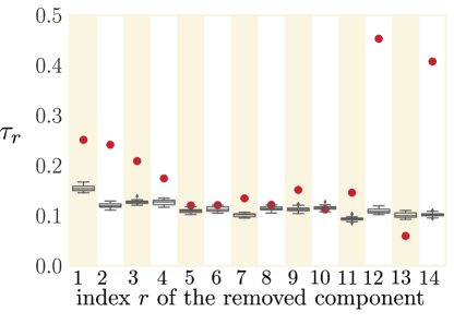
Figure 2: Epidemic delay ratio as a function of removed component. The epidemic delay ratio $\tau_{r}$ of Eq. 3 is plotted (solid circles) as a function of the removed network component and compared to the null model described in the main text (boxplots). In each boxplot, the central band is the median, the bottom and top of the box are the first and third quartiles. Whiskers extent to the most extreme data point within 1.5 IQR of the inner quartiles. Points beyond whiskers are outliers.

We observe that the delay ratio obtained by selectively removing a component (solid circles) is almost always larger than the one obtained by removing links at random (boxplots): Such targeted interventions have a stronger effect than random removals of links. For the first $9$ structures, the delay ratio is positively correlated with the component weight of Table 1, as we could naively expect. Strikingly, the removal of components $12$ or $14$ slows down the epidemic spread considerably. These two mesostructures, despite carrying a smaller total weight than most other components (see Table 1), thus appear to play a more important role for SI spreading. As shown in Fig. 1 both components $12$ and $14$ mix nodes from different classes and have activity concentrated during the lunch break of the first day. The other components correspond either to individual classes (components $1$ through $9$ and $11$) or to components, such as $10$ and $13$, with little activity on the first day. Overall, the SI process is slowed down the most by removing comparatively weak structures (in terms of weight) that mix classes and occur early in the data. We remark that the most effective intervention for mitigating epidemic spread thus involves the removal of seemingly minor mesostructures that correspond to complex correlations between link activity and network structure, and cannot be uncovered by standard community detection approaches.

We now turn to the case of an SIR process and investigate the effect of mesostructure removal on the dynamics of an SIR epidemic over the temporal network. We compute the epidemic size ratio $\rho_{\lambda,\mu}(r)$ of Eq. 4 for a wide range of values of the parameters $\lambda$ and $\mu$, and for all components $r$. The results are shown in Fig 3 for selected components and in the Supplementary Information for all the other components.

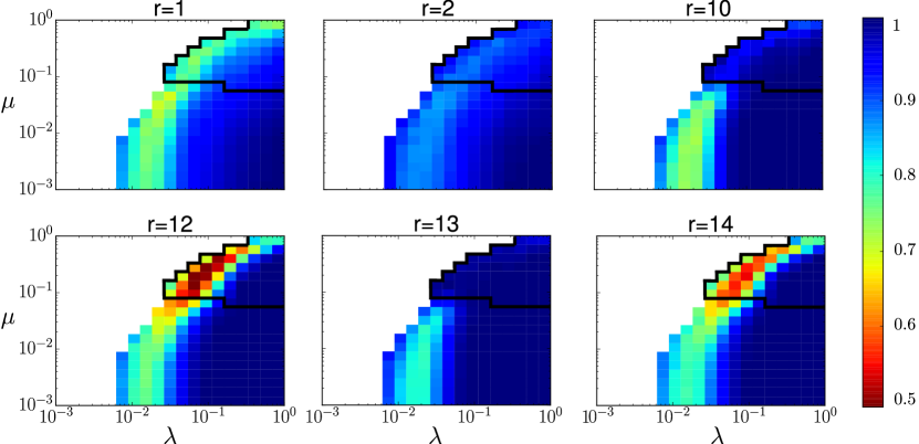
Figure 3: Epidemic size ratio as a function of SIR model parameters. Each heat map corresponds to a targeted intervention that selectively removes one component. For each removed component $r$ the heat map shows the epidemic size ratio $\rho_{\lambda,\mu}(r)$ as a function of the SIR parameters $\lambda$ and $\mu$. $\rho_{\lambda,\mu}(r)=1$ indicates that the intervention does not affect epidemic size. The white area is the region where the epidemic dies out, i.e., it fails to affect more than 1% of the network nodes. The region inside the black contour line corresponds to parameter values such that the SIR epidemic finishes within the finite span of the school dataset (2 days), both for the full and the altered temporal networks. That is, for those parameter values the epidemic size ratio is not affected by the finite temporal span of the dataset.

We notice that for large $\lambda$ values and small $\mu$ values (bottom right of the heat maps) the epidemic size ratio $\rho_{\lambda,\mu}(r)\simeq 1$: in this region the epidemics spreads and finishes fast, hence mesostructure removal cannot mitigate its size. The parameter region where mesostructure removal can have a strong effect, therefore, is the arc-shaped region visible, e.g., in the heat map for $r=1$ (lighter blue/green). The removal of class components $r=1$ and $r=2$ mildly mitigates the epidemic for a broad range of parameter within that region (almost no effect is obtained for the other class components, as shown in Fig. S4 of the Supplementary Information). Removing the class component $1$ has a comparatively higher effect because of the higher overall weight of that component (Table 1).

On taking a closer look at Fig. 3 we notice that, depending on the removed component, significant epidemic mitigation can be achieved in two main parameter regions within the arc. The first region falls within the black contour (high values of $\lambda$ and $\mu$) and corresponds to parameter values yielding epidemics that finish by the end of the second day. In this region the epidemic can be strongly mitigated ($\rho_{\lambda,\mu}\simeq 0.5$) by removing mesostructures that involve mixing of classes on the first school day, namely $r=12$ and $r=14$. This is consistent with the results of Fig. 2 for the SI case. Conversely, removing the class-mixing components $r=10$ and $r=13$, which are mostly active on the second day (Fig. 1) has a negligible effect in the same parameter region. For a sample parameter choice within this region, in Fig. 4 we illustrate the temporal evolution of the epidemics and the effect of removing individual components: the epidemic on the unmodified network peaks on the first day and, consistently with the above remarks, removing $r=12$ or $r=14$ strongly mitigates the fraction of affected nodes, whereas the removal of $r=10$ and $r=13$ has a negligible effect.

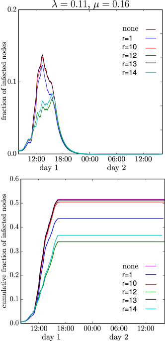
Figure 4: Fraction of infected nodes as a function of time for a sample parameter choice. Temporal evolution of the average fraction of infected nodes (top) and of the cumulative fraction of infected nodes (bottom) as a function of time for a sample parameter choice of $\lambda=0.11$ and $\mu=0.16$. The curve marked as none corresponds to the spread on the unmodified temporal network $\tilde{\mathcal{T}}$. The other curves show the effect of selectively removing components $r=1,10,11,12,14$. For the chosen parameter values, epidemic spread occurs on the first day, hence removing the early class-mixing components $r=12$ or $r=14$ has a strong mitigation effect.

We remark that removing the early class-mixing mesostructures also mitigates the SIR epidemic for a wide range of parameter values outside the black contour, as visible in Fig. 3, and that removing these mesostructures is more effective, in general, than removing class components, even though the latter account for a larger network weight. The second parameter region of interest lies in the lower part of the arc (low values of $\lambda$ and $\mu$) and is visible in Fig. 3 for $r=10$ and $r=13$. This region corresponds to parameter values for which the SIR process is slower and the epidemic does not finish over the 2-day temporal span of the data. In this case, removing either of the class-mixing mesostructures $r=10,12,13,14$ as a similar and limited effect on the epidemic size reached at the end of the second day.

Discussion

We have put forward a methodology to systematically assess the relevance of mesostructures for dynamical processes such as epidemic spread in temporal networks. The proposed method only uses time-resolved connectivity information without metadata and allows to uncover complex patterns of correlated link activity whose removal has a strong impact on simulated epidemic spreading for a broad range of model parameters. The removal of an individual mesostructure can be regarded as a targeted intervention at the mesoscale, such as the removal of a specific group of nodes or the suppression of a specific activity pattern (e.g., a lunch break). These targeted interventions have a potentially high relevance, as they do not involve the system as a whole, nor they need actions at microscopic level of individual nodes. Hence, they might strike a balance between cost and effectiveness that might make them actionable in a variety of applications.

As an illustration of the method, we have considered a case study where simple but paradigmatic spreading processes occur on top of an empirical temporal network describing face-to-face interactions in a school. In this case, the most important mesostructures for epidemic spread are not those involving most of the link activity, but instead consist of weaker, temporally-localized mixing patterns corresponding to scheduled social activities. It is important to remark that these mesostructures cannot by found by means of community detection techniques on static networks, and that our methods reveals them in an unsupervised fashion. We also notice that the actionability of an intervention that suppresses a given mesostructure hinges on the recognizability of that mesostructure in terms of relevant contextual information, such as a known or understandable grouping of nodes, temporal activity localized at specific times of a known schedule, or a specific relation to other metadata for the context at hand. For example, the selective removal of component $\mathcal{S}_{12}$ of Fig. 1 only becomes an actionable targeted intervention when its temporal activity profile is identified as a mixing pattern associated with the lunch break on the first school day.

Our work is a first step towards the systematic design of mesoscale interventions in temporal networks. Natural future steps include the use of our methodology on different temporal networks, both empirical and synthetic, the investigation of the impact of incomplete or noisy data, and the study of other dynamical processes.

Methods

A 3-mode tensor $\mathcal{T}$, with entries $T_{ijk}$, can be approximated by a sum $\tilde{\mathcal{T}}$ of $R$ rank-$1$ tensors ^{45; 32; 46},

$$\tilde{\mathcal{T}}=\sum_{r=1}^{R}\,\mathcal{S}_{r}\ =\sum_{r=1}^{R}\,\mathbf{a_{r}}\circ\mathbf{b_{r}}\circ\mathbf{c_{r}}\ ,$$ (5)

where each component tensor $\mathcal{S}_{r}$ is the outer products of three vectors, $\mathcal{S}_{r}=\mathbf{a_{r}}\circ\mathbf{b_{r}}\circ\mathbf{c_{r}}$. The Frobenius norm of the difference between $\mathcal{T}$ and $\tilde{\mathcal{T}}$, $\epsilon=\|\mathcal{T}-\tilde{\mathcal{T}}\|$, quantifies the error in approximating the original tensor with the sum $\tilde{\mathcal{T}}$. The number of components $R$ is interpreted as the number of sought mesostructures in the decomposition of the temporal network. Its value needs to be set by balancing the conflicting goals of minimizing $\epsilon$, i.e., recovering as much as possible of the original tensor, and avoiding overfitting ^{47; 32; 31}. The sets of vectors $a_{\{1,2,\dots,R\}}$, $b_{\{1,2,\dots,R\}}$, $c_{\{1,2,\dots,R\}}$ can be combined into matrices $\mathbf{A}\in\mathbb{R}^{N\times R}$, $\mathbf{B}\in\mathbb{R}^{N\times R}$ and $\mathbf{C}\in\mathbb{R}^{S\times R}$. These matrices all have $R$ columns, one for each component of the decomposition, i.e., one for each sought mesoscale structure.

For an undirected temporal network (such as the one of our case study) the adjacency matrix represented on each tensor slice is symmetric and the decomposition yields $\mathbf{A}\simeq\mathbf{B}$. In practice it is possible to directly seek a decomposition with $\mathbf{A}\equiv\mathbf{B}$, i.e., with component tensors of the form $\mathcal{S}_{r}=\mathbf{a_{r}}\circ\mathbf{a_{r}}\circ\mathbf{c_{r}}$. Hence in the main text we only refer to the matrices $\mathbf{A}$ and $\mathbf{C}$: the matrix elements $a_{ir}$ of $\mathbf{A}$ associate each component $r=1,\dots,R$ with individual nodes of the network, while the matrix elements $c_{kr}$ of $\mathbf{C}$ encode the temporal activity pattern of each component, with time indexed by $k$. The decomposition of Eq. 5 can be written as

$$T_{ijk}=\sum_{r=1}^{R}\,a_{ir}\,a_{jr}\,c_{kr}\ .$$ (6)

The matrix elements $a_{ir}$ indicate notion of membership of node $i$ to component $r$, so this representation is suitable to describe overlapping mesostructures and complex correlations between connectivity patterns and activity patterns over time. Notice that even when the original temporal network is unweighted, that is, the tensor $\mathcal{T}$ is binary-valued, the component tensors $\mathcal{S}_{r}$ correspond in general to weighted networks, and the approximating tensor $\tilde{\mathcal{T}}$ is in general real-valued.

To compute the decomposition of Eq. 5 we need to solve an optimization problem that minimizes the residual $\epsilon$. A standard way to do so is to convert the $3$-mode problem yielded by Eq. 5 into three coupled $2$-mode sub-problems: This is done by unfolding the original tensor $\mathcal{T}$ along its three modes, a technique also known as matricization ⁴⁵. Using this representation, the original tensor approximation problem is cast into $3$ coupled matrix approximation problems that involve the factor matrices $\mathbf{A}$, $\mathbf{B}$, and $\mathbf{C}$. Since the corresponding optimization problems are convex with respect to either of the matrices – but not with respect to them all – it is possible to solve the optimization through a method known as Alternative Non-negative Least Squares ⁴⁸. The minimization of $\epsilon$ is usually carried out with non-negativity and/or sparsity constraints on the factor matrices ^{45; 32}, as this is known to yield decompositions that can be interpreted as parts-based representations of the original data ⁴².

Here we carry out the decomposition with non-negativity constraints, using Alternating Non-negative Least Squares and a block-coordinate descent method to improve convergence speed ^{49; 50}. Our implementation builds on the MATLAB code of ref. 51. The number of components $R$ is set by using the core consistency diagnostic ^{47; 31} optimized over $5$ stochastic realizations of the decomposition that differ for the random initial conditions of the factor matrices. The components $\mathcal{S}_{r}$ are ordered so that the Euclidean norm of $\mathcal{S}_{r}$ decreases for increasing $r$. That is, the first column of matrices $\mathbf{A}$, $\mathbf{B}$ and $\mathbf{C}$ correspond to the component with highest Euclidean norm, and successive columns encode weaker and weaker components.

Author Contributions

All authors contributed to the manuscript. LG, AB and CC designed the study. AB and CC supervised the study. AB and CC collected and post-processed the data. LG and AP analyzed data and prepared figures. LG carried out computer simulations. LG, AB, CC wrote the manuscript. All authors reviewed the manuscript.

Additional Information

The authors declare no competing financial interests.

Supplementary Information

Properties of the decomposition of the contact network

The original temporal network $\mathcal{T}$ is decomposed by the non-negative tensor factorization method described in the Methods section and approximated by the resulting tensor $\tilde{\mathcal{T}}$, which is a sum of $R$ products of lower-dimensional factors. This approximation was carried out for several values of the number $R$ of components, i.e. of rank-$1$ tensors, in order to determine the range of values such that $R$ is large enough to describe the mesoscale properties of the original network and small enough to avoid overfitting. The core consistency, a measure introduced in ⁴⁷ and plotted in Fig. S1 for several values of the number $R$ of rank-$1$ tensors, guides the choice of a representative number of components for $\tilde{\mathcal{T}}$.

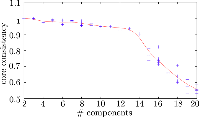
Figure S1: Core consistency curve with respect to the number of components. Each cross corresponds to a decomposition, $5$ realizations are shown for each number of components used. The line acts as a guide for the eyes.

In the case study we consider, we limit the decomposition to $R=14$ terms to avoid overfitting. In Fig. S2, we show that this number of terms is sufficient by comparing the total activity (number of interactions in the whole data set) of each node in the approximated network $\tilde{\mathcal{T}}$ and in the original network $\mathcal{T}$. As mentioned in the Methods section, $\tilde{\mathcal{T}}$ is real-valued even if $\mathcal{T}$ is binary-valued.

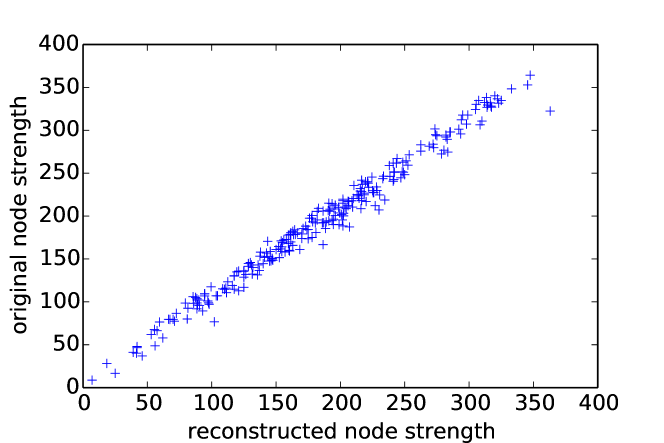
Figure S2: Cumulative node strength in the original temporal network described by $\mathcal{T}$, versus cumulative node strength in the reconstructed tensor $\tilde{\mathcal{T}}$ with $R=14$ components.

Spreading processes and intervention strategies

Both Susceptible-Infectible and Susceptible-Infectible-Recovered processes are run on the reconstructed network and the altered networks. We consider $R=14$ altered networks: the $r-$th one, $\tilde{\mathcal{T}}^{r}$, is built by excluding the $r-$th component from the sum defining $\tilde{\mathcal{T}}$.

Details of the epidemics simulations

The quantities measured for the SI process are averaged, for each altered network and for each parameter $\lambda$, over all possible seeds and for each seed over $50$ spread starting times taken between $10\%$ and $30\%$ of the total time length of the dataset. The quantities measured in the case of the SIR process are averaged, for each altered network and each set of parameters $(\lambda,\mu)$, over all possible seeds and for each seed over $10$ starting times taken between $10\%$ and $15\%$ of the total time length of the dataset.

Efficiency of targeted interventions for the SI process: effect of different propagation probabilities

Figure 2 of the main text shows the delay ratio of SI processes obtained by the selected removal of each mesostructure of the temporal network, for a specific value of the spreading rate $\lambda$. The maximal value of $\lambda$ tested is chosen such that $\lambda$ times the maximal weight of the links (here $1.1$) does not exceed $1$.

We show in Fig. S3 the results obtained with different values of $\lambda$ on each altered network together with the results obtained on $20$ realizations of associated null models. Each null model associated to an altered network is built by taking the fully reconstructed network $\tilde{\mathcal{T}}$ and zeroing out link weights at random until the sum removed is equal to the actual cumulated weights removed in the corresponding altered network $\tilde{\mathcal{T}}^{r}$. Although the efficiency of the single removal of each mesostructure depends on $\lambda$, the global picture remains unchanged: the removal of one of the mixing patterns active during the first day ($r=12$ or $r=14$) largely outperforms the removal of any of the other mesostructures as well as the random removal of an equivalent amount of activity.

Let us also note for precision that the half-infection time used in the computation of the infection delay ratio is measured starting from the time at which the seed infects a node instead of the time of its first contact (as it was done in Ref. 24). The reason is that the links of the reconstructed network are not binary (active or inactive) but carry weights, so that the precise definition of a contact is blurred and recovering a binary definition of contacts would require to set an arbitrary threshold.

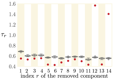
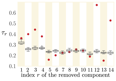
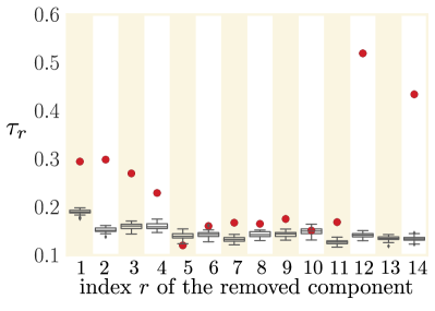
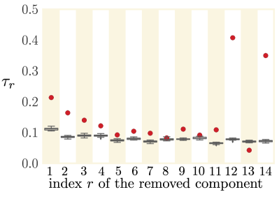
Figure S3: Measured delay ratios for SI processes simulated on top of the reconstructed network $\tilde{\mathcal{T}}$ and of the $14$ altered networks. The boxplots correspond to the delay ratios obtained by simulating SI processes on top of $\tilde{\mathcal{T}}$ and of $14$ ensemble of networks altered by random removal of interactions: for each mesostructure $r$, we remove from $\tilde{\mathcal{T}}$ weights at random under the constraint that the sum of the removed weights is equal to the sum of the weights of the component $r$. Each boxplot gives the distribution of delay ratios obtained for $20$ realizations of the random removal procedure. Horizontal lines inside each box show the median values, and each box extends from the first to the third quartile of the corresponding distribution. The reach of whiskers are determined by the sum of the third quartile and the interquartile weighted by 1.5. Points beyond the whiskers are outliers. The transmission probability of the SI processes is (a) $\lambda=0.1$, (b) $\lambda=0.3$, (c) $\lambda=0.5$, (d) $\lambda=0.9$.

Targeted intervention for the SIR process

To quantify the difference between SIR processes unfolding on top of $\tilde{\mathcal{T}}$ and on top of altered networks, we measured the averaged ratio, $\rho_{\lambda,\mu}(r)$, between the average size $\Omega^{r}$ of the epidemic on the altered network $\tilde{\mathcal{T}}^{r}$ and the average size $\Omega$ of the epidemic on the full network $\tilde{\mathcal{T}}$. To estimate the statistical significance of our results, we have performed Wilcoxon signed-rank tests for each parameter set ($\lambda,\mu,r$) comparing the epidemics size distributions pairwise between simulations performed on each altered network and on the full $\tilde{\mathcal{T}}$. The test’s result shows that either the averages of the epidemic sizes are significantly different with a $p-$value lower than $10^{-3}$, or the ratio $\rho_{\lambda,\mu}(r)$ lies between $0.99$ and $1$. Therefore, this test shows that whenever $\rho_{\lambda,\mu}(r)$ is smaller than $0.99$, the observed difference between the outcomes of the spreading processes run on $\tilde{\mathcal{T}}^{r}$ and $\tilde{\mathcal{T}}$ is significant.

We show in Fig. S4 the ratio of epidemic sizes $\rho_{\lambda,\mu}(r)$ for SIR processes simulated on top of altered networks with a mesostructure $r$ removed and on top of the whole decomposition $\tilde{\mathcal{T}}$, for the values of $r$ not shown in the main text. These mesostructures describe activities occurring in single classes, and their removal have only negligible impact on the outcome of the SIR process.

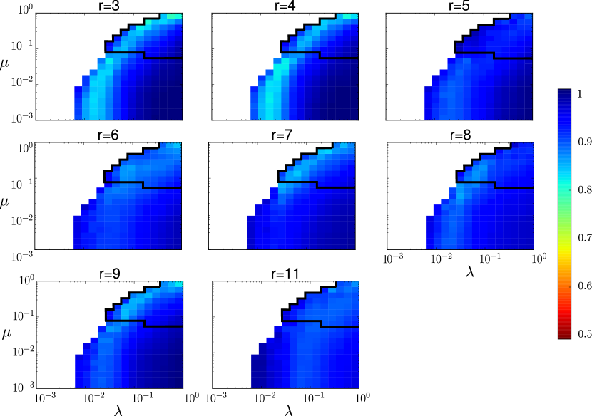
Figure S4: Ratio of epidemics sizes $\rho_{\lambda,\mu}(r)$ for SIR processes simulated on top of altered networks with a mesostructure $r$ removed and on top of the whole $\tilde{\mathcal{T}}$. The values of $r$ selected here are those which were not on Fig. 3 of the main text. The white part of each heat map corresponds to the region where the simulated epidemic process dies out. The black contour corresponds to the boundary of the parameter region such that the SIR process is over within the finite span of the dataset (i.e., to parameter values yielding epidemic processes that last at most two days): in this parameter region, the finite length of the dataset has no influence on the outcome of the epidemic.

Evolution of the epidemic size in different regimes

The temporal evolutions of the fraction of infected nodes are displayed in Fig. S5 for two sets of $(\lambda,\mu)$ chosen to be in two different regimes. In Fig. S5(a), spread and recovery are slow, and the spread is not over at the end of the dataset. The removal of any of the mixing patterns thus has a similar impact at the end of the two days, independently of the fact that their activity occurs on the first or on the second day. For the parameter values used in Fig. S5(b) on the other hand, the spread is too fast to be mitigated.

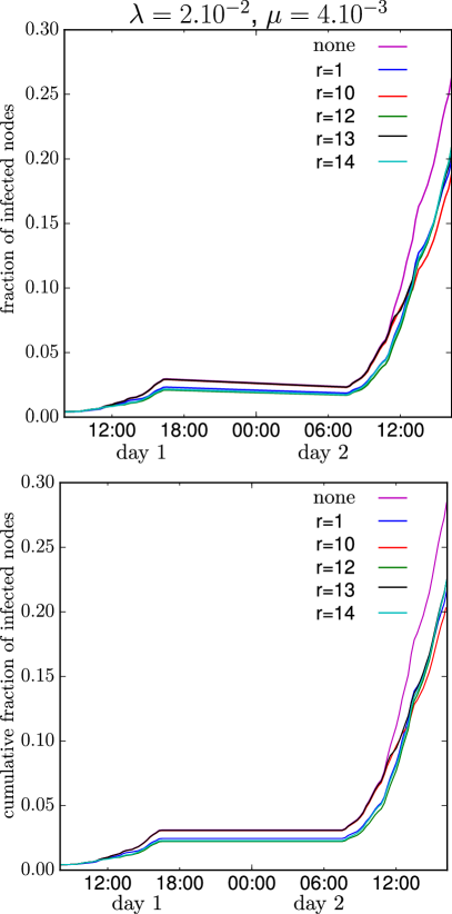
Figure S5: Temporal evolution of the average fraction of nodes in the infected states for SIR processes simulated on top of altered networks with a mesostructure $r$ removed and on top of the whole decomposition $\tilde{\mathcal{T}}$. The values of $r$ selected here are the same as in Fig. 4 of the main text, for (a) $\lambda=2.10^{-2}$ and $\mu=4.10^{-3}$ and (b) $\lambda=1.6~{}10^{-1}$ and $\mu=4.10^{-2}$. The curve marked as none corresponds to the spread on the unmodified temporal network $\tilde{\mathcal{T}}$.

References

- 1 Vespignani, A. Modelling dynamical processes in complex socio-technical systems. Nature Physics 8, 32–39 (2012).
- 2 Barrat, A., Barthelemy, M. & Vespignani, A. Dynamical processes on complex networks, vol. 1 (Cambridge University Press Cambridge, 2008).
- 3 Onnela, J.-P. et al. Structure and tie strengths in mobile communication networks. Proceedings of the National Academy of Sciences 104, 7332–7336 (2007).
- 4 Holme, P. & Saramäki, J. Temporal networks. Physics Reports 519, 97–125 (2012).
- 5 Vazquez, A., Rácz, B., Lukács, A. & Barabási, A.-L. Impact of non-poissonian activity patterns on spreading processes. Phys. Rev. Lett. 98, 158702 (2007).
- 6 Karsai, M. et al. Small but slow world: How network topology and burstiness slow down spreading. Phys. Rev. E 83, 025102 (2011).
- 7 Perra, N., Gonçalves, B., Pastor-Satorras, R. & Vespignani, A. Activity driven modeling of time varying networks. Sci. Rep. 2 (2012).
- 8 Gauvin, L., Panisson, A., Cattuto, C. & Barrat, A. Activity clocks: spreading dynamics on temporal networks of human contact. Scientific reports 3 (2013).
- 9 Rocha, L. E. C. & Blondel, V. D. Bursts of vertex activation and epidemics in evolving networks. PLoS Comput Biol 9, e1002974 (2013).
- 10 Masuda, N. & Holme, P. Predicting and controlling infectious disease epidemics using temporal networks. F1000Prime Reports 5 (2013).
- 11 Takaguchi, T., Masuda, N. & Holme, P. Bursty communication patterns facilitate spreading in a threshold-based epidemic dynamics. PLoS ONE 8, e68629 (2013).
- 12 Horváth, D. X. & Kertész, J. Spreading dynamics on networks: the role of burstiness, topology and non-stationarity. New Journal of Physics 16, 073037 (2014).
- 13 Holme, P. & Liljeros, F. Birth and death of links control disease spreading in empirical contact networks. Sci. Rep. 4 (2014).
- 14 Scholtes, I., Wider, R., N andPfitzner, Garas, A., Tessone, C. & Schweitzer, F. Causality-driven slow-down and speed-up of diffusion in non-markovian temporal networks. Nat. Comm 5, 5024 (2014).
- 15 Backlund, V.-P., Saramäki, J. & Pan, R. K. Effects of temporal correlations on cascades: Threshold models on temporal networks. Phys. Rev. E 89, 062815 (2014).
- 16 Perotti, J. I., Jo, H.-H., Holme, P. & Saramäki, J. Temporal network sparsity and the slowing down of spreading. preprint arXiv:1411.5553 (2014).
- 17 Eagle, N. & Pentland, A. Reality mining: sensing complex social systems. Personal and ubiquitous computing 10, 255–268 (2006).
- 18 Salathé, M. et al. A high-resolution human contact network for infectious disease transmission. Proceedings of the National Academy of Sciences 107, 22020–22025 (2010).
- 19 Cattuto, C. et al. Dynamics of person-to-person interactions from distributed rfid sensor networks. PLoS ONE 5, e11596 (2010).
- 20 Stopczynski, A. et al. Measuring large-scale social networks with high resolution. PLoS ONE 9, e95978 (2014). URL http://dx.doi.org/10.1371%2Fjournal.pone.0095978.
- 21 Stehlé, J. et al. Simulation of an seir infectious disease model on the dynamic contact network of conference attendees. BMC medicine 9, 87 (2011).
- 22 Lee, S., Rocha, L. E. C., Liljeros, F. & Holme, P. Exploiting temporal network structures of human interaction to effectively immunize populations. PLoS ONE 7, e36439 (2012).
- 23 Gemmetto, V., Barrat, A. & Cattuto, C. Mitigation of infectious disease at school: targeted class closure vs school closure. BMC infectious diseases 14, 3841 (2014).
- 24 Starnini, M., Machens, A., Cattuto, C., Barrat, A. & Pastor-Satorras, R. Immunization strategies for epidemic processes in time-varying contact networks. Journal of theoretical biology 337, 89–100 (2013).
- 25 Liu, S., Perra, N., Karsai, M. & Vespignani, A. Controlling contagion processes in activity driven networks. Phys. Rev. Lett. 112, 118702 (2014).
- 26 Bajardi, P., Barrat, A., Natale, F., Savini, L. & Colizza, V. Dynamical patterns of cattle trade movements. PloS one 6, e19869 (2011).
- 27 Fortunato, S. Community detection in graphs. Physics Reports 486, 75 – 174 (2010).
- 28 Salathé, M. & Jones, J. H. Dynamics and control of diseases in networks with community structure. PLoS computational biology 6, e1000736 (2010).
- 29 Almendral, J. A., Criado, R., Leyva, I., Buldú, J. M. & Sendiña-Nadal, I. Introduction to focus issue: Mesoscales in complex networks. Chaos: An Interdisciplinary Journal of Nonlinear Science 21, – (2011). URL http://scitation.aip.org/content/aip/journal/chaos/21/1/10.1063/1.3570920.
- 30 Mucha, P. J., Richardson, T., Macon, K., Porter, M. A. & Onnela, J.-P. Community structure in time-dependent, multiscale, and multiplex networks. Science 328, 876–878 (2010).
- 31 Gauvin, L., Panisson, A. & Cattuto, C. Detecting the community structure and activity patterns of temporal networks: a non-negative tensor factorization approach. PLOS ONE 9, e86028 (2014).
- 32 Kolda, T. G. & Bader, B. W. Tensor decompositions and applications. SIAM Rev. 51, 455–500 (2009).
- 33 Longini, I. J., Koopman, J., Monto, A. & Fox, J. Estimating household and community transmission parameters for influenza. Am J Epidemiol 115(5), 736–51 (1982).
- 34 Viboud, C. et al. Risk factors of influenza transmission in households. Br J Gen Pract 54(506), 684–9 (2004).
- 35 Chao, D. L., Halloran, M. E. & Longini, I. M. School opening dates predict pandemic influenza A (H1N1) outbreaks in the united states. Journal of Infectious Diseases 202, 877–880 (2010).
- 36 Lee, B. Y. et al. Simulating school closure strategies to mitigate an influenza epidemic. Journal of public health management and practice: JPHMP 16, 252 (2010).
- 37 Baguelin, M. et al. Assessing optimal target populations for influenza vaccination programmes: An evidence synthesis and modelling study. PLoS Med 10, e1001527 (2013).
- 38 Cauchemez, S. et al. Closure of schools during an influenza pandemic. The Lancet Infectious Diseases 9, 473 – 481 (2009).
- 39 Brown, S. et al. Would school closure for the 2009 H1N1 influenza epidemic have been worth the cost?: a computational simulation of pennsylvania. BMC Public Health 11, 353 (2011).
- 40 Dalton, C., Durrheim, D. & Conroy, M. Likely impact of school and childcare closures on public health workforce during an influenza pandemic: a survey. Commun Dis Intell 32(2), 261262 (2008).
- 41 De Domenico, M. et al. Mathematical formulation of multilayer networks. Physical Review X 3, 041022 (2013).
- 42 Lee, D. D. & Seung, H. S. Learning the parts of objects by non-negative matrix factorization. Nature 401, 788–791 (1999).
- 43 Yang, J. & Leskovec, J. Overlapping community detection at scale: a nonnegative matrix factorization approach. In Proceedings of the sixth ACM international conference on Web search and data mining, WSDM ’13, 587–596 (ACM, New York, NY, USA, 2013).
- 44 Stehlé, J. et al. High-resolution measurements of face-to-face contact patterns in a primary school. PLOS ONE 6, e23176 (2011).
- 45 Cichocki, A., Zdunek, R., Phan, A.-H. & Amari, S. Nonnegative Matrix and Tensor Factorizations: Applications to Exploratory Multi-way Data Analysis and Blind Source Separation (John Wiley & Sons, Ltd, 2009).
- 46 Mørup, M. Applications of tensor (multiway array) factorizations and decompositions in data mining. Wiley Interdisc. Rew.: Data Mining and Knowledge Discovery 1, 24–40 (2011).
- 47 Bro, R. & Kiers, H. A. L. A new efficient method for determining the number of components in parafac models. Journal of Chemometrics 17, 274–286 (2003).
- 48 Paatero, P. & Tapper, U. Positive matrix factorization: A non-negative factor model with optimal utilization of error estimates of data values. Environmetrics 5, 111–126 (1994).
- 49 Kim, J. & Park, H. Fast nonnegative tensor factorization with an active-set-like method. In Berry, M. W. et al. (eds.) High-Performance Scientific Computing, 311–326 (Springer London, 2012).
- 50 Kim, J., He, Y. & Park, H. Algorithms for nonnegative matrix and tensor factorizations: A unified view based on block coordinate descent framework. Journal of Global Optimization 58, 285–319 (2014).
-
51
http://www.cc.gatech.edu/~hpark/software/ntf_package.zip,
accessed on 1/6/2015.