Revisiting Ulysses Observations of Interstellar Helium

Abstract

We report the results of a comprehensive reanalysis of Ulysses observations of interstellar He atoms flowing through the solar system, the goal being to reassess the interstellar He flow vector and to search for evidence of variability in this vector. We find no evidence that the He beam seen by Ulysses changes at all from 1994–2007. The direction of flow changes by no more than $\sim 0.3^{\circ}$ and the speed by no more than $\sim 0.3$ km s^-1. A global fit to all acceptable He beam maps from 1994–2007 yields the following He flow parameters: $V_{ISM}=26.08\pm 0.21$ km s^-1, $\lambda=75.54\pm 0.19^{\circ}$, $\beta=-5.44\pm 0.24^{\circ}$, and $T=7260\pm 270$ K; where $\lambda$ and $\beta$ are the ecliptic longitude and latitude direction in J2000 coordinates. The flow vector is consistent with the original analysis of the Ulysses team, but our temperature is significantly higher. The higher temperature somewhat mitigates a discrepancy that exists in the He flow parameters measured by Ulysses and the Interstellar Boundary Explorer, but does not resolve it entirely. Using a novel technique to infer photoionization loss rates directly from Ulysses data, we estimate a density of $n_{\rm He}=0.0196\pm 0.0033$ cm^-3 in the interstellar medium.

1 INTRODUCTION

The global structure of the heliosphere is determined in large part by the local ISM flow vector in the rest frame of the Sun. Older determinations of this vector, particularly those based on measurements of interstellar He flowing through the inner heliosphere by the GAS instrument on Ulysses, have recently been challenged by new measurements of the He flow by the Interstellar Boundary Explorer (IBEX). The canonical Ulysses analysis of Witte (2004) suggested the following He flow parameters: $V_{ISM}=26.3\pm 0.4$ km s^-1, $\lambda=75.4\pm 0.5^{\circ}$, $\beta=-5.2\pm 0.2^{\circ}$, and $T=6300\pm 340$ K; where $\lambda$ and $\beta$ are the ecliptic longitude and latitude direction in J2000 coordinates. In contrast, IBEX data recently yielded the following flow properties (Bzowski et al., 2012; Möbius et al., 2012; McComas et al., 2012): $V_{ISM}=23.2\pm 0.3$ km s^-1, $\lambda=79.00\pm 0.47^{\circ}$, $\beta=-4.98\pm 0.21^{\circ}$, and $T=6300\pm 390$ K. Significant inconsistencies exist between the Ulysses and IBEX measurements, particularly for $V_{ISM}$ and $\lambda$.

The lower $V_{ISM}$ value of IBEX is of particular interest, as it may imply the nonexistence of a bow shock around the heliosphere. The $V_{ISM}=23-27$ km s^-1 interstellar flow speed happens to imply a fast magnetosonic Mach number of $M_{F}\approx 1$, making the existence or nonexistence of a bow shock around the heliosphere very much an open question. Uncertainties in the strength and orientation of the interstellar magnetic field, $B_{ISM}$, represent one obstacle in determining whether a bow shock exists. The higher $B_{ISM}$ is (and the more perpendicular to the ISM flow), the lower $M_{F}$ should be, and the less likely there is to be a bow shock. But uncertainties in $V_{ISM}$ are also important.

For many years the best assessments of ISM velocity suggested $V_{ISM}\approx 26$ km s^-1, not only the Ulysses/GAS measurements (Witte et al., 1996; Witte, 2004) but measurements from ISM absorption lines as well ($V_{ISM}=25.7\pm 0.5$ km s^-1; Lallement & Bertin 1992). With these relatively high values, heliospheric modelers favored $M_{F}>1$, implying the existence of a bow shock. However, not only has the new IBEX measurement called this into question, but so has one reanalysis of ISM absorption line data (Redfield & Linsky, 2008), which suggests $V_{ISM}=23.84\pm 0.90$ km s^-1. The lower $V_{ISM}=23-24$ km s^-1 values reported recently have been enough for many to argue that $M_{F}<1$ should be preferred (McComas et al., 2012; Zieger et al., 2013). However, Scherer & Fichtner (2014) argue that including He⁺ density in the calculation of Alfvén speeds instead of just assuming a pure proton plasma would still suggest $M_{F}>1$ even if $V_{ISM}\approx 23$ km s^-1. On the other hand, Zank et al. (2013) note that charge exchange processes may turn the bow shock into more of a “bow wave” even if $M_{F}>1$.

In any case, the existence or nonexistence of a heliospheric bow shock is one issue driving interest in whether the He flow vector of Ulysses or that of IBEX is to be preferred. Assuming that the ISM cloud around the Sun is nonrigid, Gry & Jenkins (2014) have reanalyzed ISM absorption line data and infer cloud kinematics more consistent with the Ulysses velocity being valid close to the Sun. Ben-Jaffel et al. (2013), Lallement & Bertaux (2014), and Vincent et al. (2014) have recently made additional arguments in favor of the older Ulysses vector, implying that the IBEX measurements must somehow be in error. Frisch et al. (2013) propose a very different solution. They propose that the local ISM flow actually varies with time, and that these variations are responsible for the Ulysses/IBEX discrepancy. However, observations of interstellar H from the Solar Wind Anisotropies instrument on the Solar and Heliospheric Observatory and the Space Telescope Imaging Spectrograph instrument on the Hubble Space Telescope do not provide support for a variable ISM flow vector (Vincent et al., 2014).

All this attention on the He flow vector provides motivation for taking another long look at the old Ulysses/GAS data, in order to see if a new, independent analysis confirms the Witte (2004) results, and to see if there is any evidence for He flow variability in the Ulysses data that would support the Frisch et al. (2013) interpretation favoring a variable ISM flow vector. Further justification is that while the Witte (2004) analysis considered data taken from 1990–2002, later data acquired up until the end of the Ulysses mission in 2007 were not considered.

Katushkina et al. (2014) have recently analyzed a couple of Ulysses He beam maps, including one from 2007, demonstrating that the new IBEX He vector cannot reproduce either map. They also note that the Witte (2004) vector might in principle be able to fit the IBEX data if the temperature is allowed to be $\sim 9000$ K, consistent with more extensive IBEX analyses (Bzowski et al., 2012; Möbius et al., 2012; McComas et al., 2012). We here present our own comprehensive reanalysis of the full Ulysses/GAS data set, providing a new assessment of the He flow vector using analysis techniques developed independently from both the original Ulysses/GAS team (Witte et al., 1996) and the IBEX team (Bzowski et al., 2012; Möbius et al., 2012).

2 THE ULYSSES DATA

Launched in 1990 October, the primary mission of the Ulysses spacecraft was to study various interplanetary constituents like the solar wind, magnetic fields, radio waves, dust, solar and galactic cosmic rays, etc. outside the ecliptic plane in an orbit passing over the solar poles (Wenzel et al., 1992; Marsden, 2001). This orbit was accomplished with a gravitational assist from Jupiter in 1992 February, leading to an orbit nearly perpendicular to the ecliptic plane, with an aphelion near Jupiter’s distance of 5 AU, and a perihelion near 1 AU. Ulysses continued to make observations from this orbit until the mission ended in late 2007. The Ulysses/GAS instrument, described in detail by Witte et al. (1992), was designed primarily to study interstellar neutral He atoms flowing through the inner heliosphere. Neutral helium provides the best diagnostic of the undisturbed ISM flow due to the high abundance of helium, and due to the fact that helium is not greatly affected by charge exchange during its journey through the outer heliosphere, in contrast to hydrogen and oxygen, for example.

The first He observations were made by Ulysses/GAS during its cruise phase out to Jupiter (1990–1992). These data were first studied by Witte et al. (1993). However, in this paper we will focus on data taken during the operational phase of the Ulysses mission, with Ulysses in its polar orbit after the Jupiter encounter. These He data are generally of higher quality than the cruise phase data (Witte, 2004), with better sampling of the He beam. Additional advantages of the operations phase data will become very clear below.

Successful detection of interstellar He required that the inflow velocity be high enough for the He atoms to exceed the particle detection threshold of the GAS instrument. With the Ulysses orbital plane being basically perpendicular to the ISM flow vector, the detectability of He depended mostly on the spacecraft velocity. Only when Ulysses was in the near-Sun part of its orbit was the spacecraft traveling rapidly enough so that the incoming He had sufficient energy to exceed the detection threshold. Thus, the Ulysses/GAS He observations were confined to the three fast latitude scans made by Ulysses, in the periods 1994–1996, 2000–2002, and 2006–2007. These are the three epochs that we will focus on here. Witte (2004) considered the first two epochs of observations, but not the last epoch.

The GAS device works essentially like a pin-hole camera with a single-element detector, so observing the He beam requires making many different exposures in different directions to fully map out the count rate distribution. The Ulysses spin axis, which was always pointed towards Earth, defined how this was done. Ulysses had a rotation period of 12 s. During this period, the GAS instrument would observe at a particular elevation angle, measured relative to the spin axis, mapping out a ring on the celestial sphere. Detected counts were accumulated in 32 bins, which could uniformly cover the full $360^{\circ}$ rotation; or more commonly cover smaller arcs of $90^{\circ}$, $45^{\circ}$, or $22.5^{\circ}$. After a period of typically 68 min, the elevation angle scanned by GAS would be changed by a step of $1^{\circ}$, $2^{\circ}$, $4^{\circ}$, or $8^{\circ}$; allowing another arc to be observed. Over the course of $2-3$ days, typically, a full scan across the He beam would be completed, and a new map begun.

The GAS instrument actually utilized two different channels with independent detectors, one with a wide field of view (WFOV) and one with a narrow field of view (NFOV), and both channels were exposed simultaneously. Over the course of the three fast latitude scans mentioned above, Ulysses obtained $\sim 400$ WFOV maps and $\sim 400$ NFOV maps. We will be working almost exclusively with the WFOV data here, which have higher signal-to-noise (S/N) than the NFOV maps.

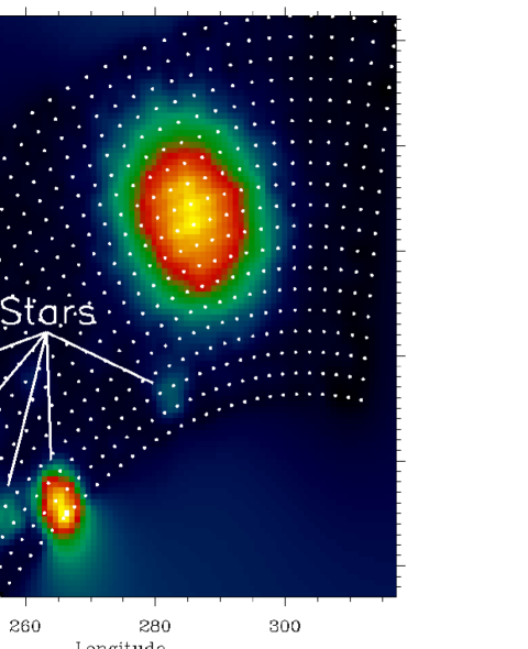
Figure 1: A WFOV helium beam map made by Ulysses/GAS on 2001 January 24, in ecliptic coordinates. White dots indicate actual scan positions used to make the map. In addition to the broad He beam, several stars are also visible.

Figure 1 shows a typical WFOV map, from 2001 January 24. The GAS instrument suffers from some sensitivity to UV emission even when in its particle detection mode (Witte et al., 1996), so some hot stars are visible in the map, in addition to the broad He beam. The stars can be inconvenient if blended with the He beam, but are actually useful as calibrators of pointing accuracy otherwise. In this article we will in fact be using a recent recalibration of the Ulysses/GAS data set making extensive use of the stars as pointing calibrators, which is described in more detail by Bzowski et al. (2014). In an end-to-end test, the calibration of the direction determination was adjusted so that the positions of stars observed by the instrument coincided with their astronomical position. Based on many more star observations from the whole mission a minor further adjustment of a few tenth of a degree was required and subsequently all He data were reprocessed in 2013 with this new calibration. This recalibration provides yet another motivation for reanalyzing these data, though the change in the data is modest. Note that although the archival Ulysses data, and its original analyses reported in the Witte et al. series of papers, are in B1950 coordinates, the numbers and figures we provide in this article will be in the more modern J2000 system.

A final distinction to be made is that we will only be considering observations of the so-called “direct beam” formed by He atoms that flow directly to the detector (with modest gravitational deflection), as opposed to the “indirect beam” created by particles that go around the Sun and are gravitationally redirected back towards the detector, arriving from a very different direction than the direct beam atoms. The indirect beam is much fainter than the direct beam due to massive photoionization and electron-impact ionization losses that occur when these particles pass close to the Sun. Ulysses has nevertheless detected the indirect beam in observations from 1995 (Witte, 2004), but we will not be considering those data here.

3 EMPIRICAL ANALYSIS

Rather than immediately try to extract a He flow vector from the data, which requires a somewhat complex forward modeling analysis (see Sections 4 and 5), we find it worthwhile to first make some purely empirical investigations of the beam. The primary motivation for this is to look for any evidence that the beam is changing at all during the 1994-2007 time period. We quantify the properties of the beam using 2-D Gaussian fits to the beam, as mapped into ecliptic coordinates (as in Figure 1). Note that there is no physical reason the beam should be precisely Gaussian, but in practice the beams observed by Ulysses are reasonably Gaussian in shape, so this is a practical way to quantify them. An example Gaussian fit is shown in Figure 2. There are six free parameters of such a fit: the central longitude and latitude, the latitudinal and longitudinal widths [specifically the full-width-at-half-maximum (FWHM)], the count rate amplitude at beam center, and a background count rate; where we assume a flat background underneath the He beam.

In the following discussion, we make use of an orbital phase for Ulysses, $\phi$, based on the angle defined by the positions of the spacecraft and the Sun, and the location of the ecliptic plane crossing near aphelion. In this system, the ecliptic plane crossing near aphelion at ecliptic coordinates ($\lambda$,$\beta$)=($157.4^{\circ}$,$0^{\circ}$) is at $\phi=0.0$, and that near perihelion at ($337.4^{\circ}$,$0^{\circ}$) is at $\phi=0.5$. The $\phi=0.25$ and $\phi=0.75$ orbital phases correspond to the near south pole and near north pole locations (relative to the Sun), so Ulysses is below the ecliptic at $\phi<0.5$ and above it at $\phi>0.5$. (Ulysses travels from south to north during its fast latitude scans.)

The Gaussian fits are performed using a semi-automated procedure, but all the fits are visually verified. Many beam maps end up being excluded for various reasons. At $\phi<0.2$ and $\phi>0.9$ the data are simply deemed too noisy. Observations with $\phi<0.26$ are excluded due to contamination from a star (specifically the rightmost star seen in Figure 1). Some maps are excluded for having a background that is not flat, possibly due to solar activity at that time. The most common reason for exclusion is simply that some scans did not fully cover the He beam. We only want to consider beam maps where the scan fully encompasses the He beam. Ultimately, fits are accepted for 234 NFOV maps and 238 WFOV maps, including the map in Figure 1. As mentioned above, we will be focusing on the higher S/N WFOV data, but we always do verify that results are not different when considering the NFOV data instead.

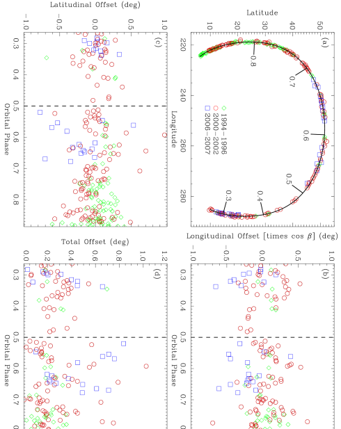
Figure 3: (a) The center of the helium beam as measured by the 2-D Gaussian fits, in ecliptic coordinates, with different symbols indicating measurements from the three different fast latitude scans. During the course of a fast latitude scan the He beam traces out this horseshoe pattern in the sky. The solid line is a polynomial fit to this horseshoe. The numbers along the horseshoe indicate orbital phase, where an orbital phase of 0.5 corresponds to the ecliptic plane crossing near perihelion. (b) Longitudinal discrepancies from the average beam location shown in (a), with the dashed line indicating the ecliptic plane crossing. (c) Latitudinal discrepancies from the average beam location. (d) Total angular offset from the average beam location.

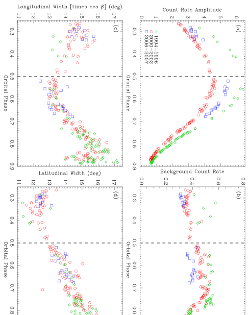
Figure 4: (a) Peak count rate amplitude of the helium beam based on the 2-D Gaussian fits, as a function of orbital phase, where an orbital phase of 0.5 corresponds to the ecliptic plane crossing near perihelion (dashed line). Different symbols indicate measurements from the three different fast latitude scans. The count rates shown are in cts s^-1 pixel^-1. The other three panels show (b) background count rates, (c) longitudinal beam widths, and (d) latitudinal beam widths.

The Gaussian fit parameters of the WFOV maps are plotted in Figures 3 and 4. Figure 3a shows that the He beam traces out a horseshoe pattern in the sky during a fast latitude scan. Performing polynomial fits to longitude and latitude as a function of orbital phase allows us to define the average beam location illustrated in Figure 3a. We will emphasize below how the shape of this horseshoe is a powerful diagnostic for the He flow parameters. Figure 3a demonstrates that basically the same horseshoe pattern is made during all three fast latitude scans, showing little indication for variation in beam location. Figures 3b-d provide a better indication for the deviations of beam position about the average. The scatter of the data points is indicative of the measurement uncertainties, but some systematic deviations are discernible despite the scatter. For example, the beam longitude appears to be lower during epoch 3 by a few tenths of a degree. The beam latitude is also a few tenths of a degree lower during epoch 3, but only for $\phi=0.5-0.7$. The latitudes observed during epochs 1 and 2 are discrepant for $\phi=0.75-0.85$.

Of particular interest are longitude variations, as it is in longitude that the IBEX and Ulysses flow vectors are in disagreement, and it is in longitude that Frisch et al. (2013) claim evidence for a systematic increase with time. There is, however, no evidence for any increase in longitude during the Ulysses era, with the epoch 3 data suggesting if anything a slight decrease, as noted above. The average discrepancy in Figure 3d is $0.28^{\circ}$. This can be interpreted as an estimate of the pointing uncertainties inherent in the Ulysses data, consistent with expectations based on the pointing calibration done using stars (Witte, 2004; Bzowski et al., 2014).

In any case, the longitude variations in Figure 3b are much smaller than the $3.6^{\circ}$ discrepancy in longitude between the IBEX and Ulysses He flow vectors. We conclude that there is no indication from the Ulysses data to support the notion that He flow variability is responsible for the IBEX/Ulysses discrepancy. Furthermore, given that we now know that the 2007 Ulysses data are not more consistent with the IBEX results than the older data, there is only a 2 year time gap between the Ulysses and IBEX eras for the He flow to have changed so significantly.

Figures 4c-d also demonstrate that there is no evidence for any significant change in the He beam shape from 1994–2007. The latitudinal and longitudinal beam widths change with orbital phase, but the same sort of variation is observed during all three fast latitude scans. Figures 4a-b show that the three epochs do, however, exhibit noticeable differences in background and beam amplitude. The Ulysses/GAS background is a complicated mix of solar and cosmic sources, and we will not discuss it much here, other than to note that both orbital phase and epochal variations are indicated by Figure 4b.

As for the beam count rate amplitude in Figure 4a, it naturally peaks near $\phi=0.5$ during each fast latitude scan, as that is when the spacecraft is moving fastest. The different count rate levels observed during the three epochs are most naturally interpreted as being indicative of variations in the solar EUV photoionization rate. It makes perfect sense for epoch 2 (2000–2002) to have the lowest He fluxes, as this is a time near solar maximum, with high photoionization rates and therefore substantial losses of neutral He due to photoionization. In contrast, epochs 1 and 3 are both near solar minimum, thereby minimizing photoionization losses. We will return to the related issues of photoionization and He density, $n_{\rm He}$, in Section 5.

4 MEASURING THE ULYSSES He FLOW VECTOR

The simple quantification of the He beam properties provided by the Gaussian fitting in the previous section is not helpful for actually inferring a He flow vector from He beam maps, which instead requires a forward modeling approach. In this procedure, a Maxwellian He velocity distribution is assumed at infinity, characterized by five parameters ($n_{\rm He}$, V_ISM, $\lambda$, $\beta$, T), and then this Maxwellian is propagated to the position of the spacecraft. The distribution will be primarily affected by the Sun’s gravitational influence. Loss processes can also be accounted for in this forward modeling, the most important being photoionization by solar EUV photons. We will initially ignore photoionization in our forward modeling, but we will consider it later to see if it changes our inferred He flow parameters.

The forward modeling method utilized in the original Ulysses/GAS team analyses is described by Banaszkiewicz et al. (1996). Our forward modeling routine, which is described in detail elsewhere (Müller & Cohen, 2012; Müller, 2012; Müller et al., 2013), involves a rather different approach to the problem than the usual method involving numerical integration from infinity. In our computations, quantities that are conserved along a trajectory, such as total energy, angular momentum, eccentricity, and direction of perihelion, are used to determine in one algebraic step the neutral He velocity at a desired point in space when its velocity at infinity is given. Conversely, when both location and velocity of a He atom are given, the conservation equations dictate a unique corresponding velocity at infinity. The entire phase space distribution, F(v), can be calculated at a desired point in the inner heliosphere by decomposing the problem into a family of trajectories with different velocities (different conserved quantities) that all converge at the chosen point. By assuming a thermal Maxwellian as the original distribution at infinity, each of those trajectories can then be assigned its corresponding phase space density, yielding F(v) at the point of interest (Müller & Cohen, 2012; Müller, 2012; Müller et al., 2013).

Computing count rates in a given direction involves first transforming F(v) into the spacecraft rest frame and converting into a coordinate system defined around the view direction of interest, resulting in F($V_{s}$,$\theta$,$\psi$), where $V_{s}$ is the speed relative to the spacecraft, $\theta$ is the poloidal angle with respect to the view direction, and $\psi$ is the azimuthal angle. With a volume element “$d^{3}v=V_{s}^{2}\sin{\theta}~{}dV_{s}~{}d\psi~{}d\theta$”, the predicted count rate can then be expressed as

$$C=A\int V_{s}~{}D_{e}(V_{s})~{}G(\theta)~{}F(V_{s},\theta,\psi)~{}d^{3}v,$$ (1)

where $A=0.0908$ cm² is the effective area, $D_{e}(V_{s})$ is the detection efficiency, and $G(\theta)$ is the detector geometry function. Figure 5 shows our digitized versions of $G(\theta)$ and $D_{e}$, approximated from Figures 1 and 3 of Banaszkiewicz et al. (1996), with the latter expressed as a function of incoming particle energy, $E_{s}=\frac{1}{2}mV_{s}^{2}$, with $m$ being the mass of the He atom. For a given elevation angle, particles in the azimuthal bins described in Section 2 are observed while the spacecraft is spinning, so there is “scan smoothing” along the azimuthal direction. We account for this by averaging $C$ values computed at pixel center and at $\pm\Delta\alpha/2$, where $\Delta\alpha$ is the azimuthal angular bin size.

By computing $C$ for all $n$ observed directions, we compute a synthetic He beam map, $C_{i}$ (for i=1,n), for comparison with the real one. This synthetic beam is multiplied by a normalization factor, $N$, in order to best match the count rates of the observed beam. This amounts to a revision of the assumed $n_{\rm He}$ value to $n^{\prime}_{\rm He}=N\times n_{\rm He}$. In making this normalization we are in effect replacing $n_{\rm He}$ with $N$ as the true density-related free parameter of our fit. We also have to account for the background count rate, $B$. As we did in the Gaussian fitting, we simply assume a flat background. Thus, the new predicted count rates are

$$C^{\prime}_{i}=N\times C_{i}+B.$$ (2)

We perform a $\chi^{2}$ minimization (e.g., Bevington & Robinson, 1992) to determine the $N$ and $B$ values that lead to the best fit to the data. The $\chi^{2}$ value of this best fit represents our measure of merit for this particular synthetic He beam map, which can be expressed as

$$\chi^{2}=\sum_{i=1}^{n}\left(\frac{S_{i}-C^{\prime}_{i}}{\sigma_{i}}\right)^{2},$$ (3)

where $C^{\prime}_{i}=C^{\prime}_{i}[N,B,C_{i}(V_{ISM},\lambda,\beta,T)]$ are the predicted count rates, $S_{i}$ are the observed count rates, $\sigma_{i}$ their Poissonian uncertainties, and $n$ the number of points considered in the He beam map. We then have to determine what He flow parameters ($V_{ISM}$, $\lambda$, $\beta$, and T) truly minimize $\chi^{2}$, representing the best fit to the data.

The standard approach for determining a set of best-fit parameters is to start with a guess for the parameters, compute $\chi^{2}$, and then use a $\chi^{2}$ minimization routine to refine the parameters to reduce $\chi^{2}$ until ultimately the true $\chi^{2}$ minimum is reached. If $\nu$ is the number of degrees of freedom of the fit (the number of data points minus the number of free parameters), then the reduced chi-squared is defined as $\chi^{2}_{\nu}=\chi^{2}/\nu$, which should be $\sim 1$ for a good fit. We use the Marquardt method described by Press et al. (1989) as our $\chi^{2}$ minimization routine.

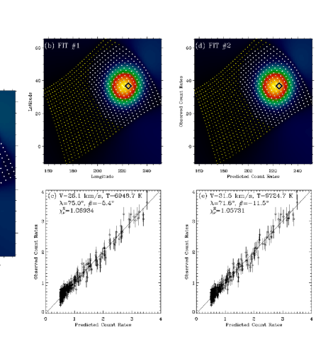
Figure 6: (a) A WFOV helium beam map from 1995 August 20, in ecliptic coordinates. The diamond indicates the expected beam position based on the Witte (2004) vector (assuming $T=0$ K). Yellow dots are scan positions, and white dots are the measurements within $25^{\circ}$ of the diamond, which are the data considered in fits. (b) A synthetic image representing a fit to the image (FIT #1) in (a), where the Witte (2004) vector was the initial guess for the best-fit parameters. (c) Observed versus predicted count rates for the fit from (b). Parameters of this fit are listed, as well as the reduced $\chi^{2}$ value ($\chi^{2}_{\nu}=1.06934$). (d) Another fit (FIT #2) to the data with a very different initial guess for the fit parameters from (b). (e) Analogous to (c) but for FIT #2. Note the very different best-fit parameters compared to (c).

Figure 6a shows a WFOV map from 1995 August 20, and Figure 6b-c shows a fit to this map, with the Witte (2004) vector used as our initial guess for the fit parameters. It is a simple matter for the particle tracking code mentioned above (Müller & Cohen, 2012; Müller, 2012) to compute the expected beam location based on the Witte (2004) vector, if we assume $T=0$ K (meaning all He atoms have the exact same velocity and follow the exact same trajectory). We use this prediction to define the map region to be fitted. In particular, we only consider data points within $25^{\circ}$ of this location (white dots in the figure), which encompasses enough of the region beyond the He beam to estimate the background. Figure 6b shows the synthetic beam map of the best fit, and Figure 6c explicitly plots observed versus predicted count rates, with a data point plotted for each of the white dots in Figure 6b. The He flow vector parameters listed in Figure 6c are gratifyingly close to the Witte (2004) vector, and the $\chi^{2}_{\nu}=1.06934$ value indicates an excellent quality fit.

Unfortunately, the best-fit parameters that we infer are actually highly dependent on our initial guesses for the parameters. This is shown explicitly in a second fit to the 1995 August 20 data in Figure 6d-e. With an initial guess very different from the Witte (2004) vector used in Figure 6b-c, we end up with a fit to the data with very different parameters. The parameters listed in Figure 6e are very far from all modern estimates of the local ISM flow vector, so we know they are wrong. But these parameters lead to a fit that is just as good as the more plausible fit in Figure 6b, with a $\chi^{2}_{\nu}=1.05731$ value that is actually slightly lower even.

This exercise emphasizes just how difficult it is to find a unique He flow vector from a single He beam map. A single map does not sufficiently constrain the problem. There are significant degeneracies among the fit parameters, leading to long diagonal troughs in $\chi^{2}$ space where it is very hard to find the true $\chi^{2}$ minimum along the trough. This is true for the analysis of IBEX data as well (see Figure 22 in Bzowski et al., 2012). The most basic degeneracy is between flow direction and flow speed, which can be explained by the following question: If a beam is seen from a given direction, is that due to a fast beam coming from roughly that direction, or due to a slower beam that has been gravitationally deflected into that direction? Since the He flow vector happens to lie near the ecliptic plane, this degeneracy basically ends up mostly between $V_{ISM}$ and $\lambda$ (rather than $\beta$).

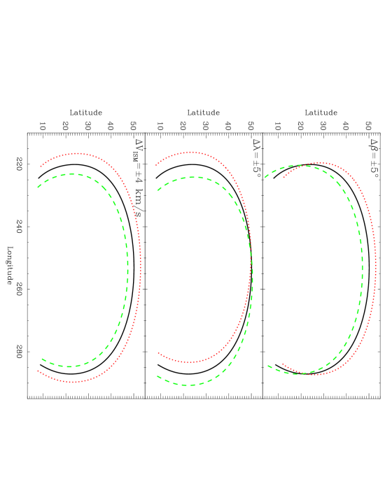
Figure 7: The solid line in each panel indicates the variation of He beam location with orbital phase expected from the Witte (2004) flow vector. Also shown in each panel is what happens to this horseshoe-shaped beam track when the latitude ($\beta$), longitude ($\lambda$), or velocity ($V_{ISM}$) of the vector are increased (dashed lines) or decreased (dotted lines) by the amount indicated.

We argue here that these degeneracies can be effectively broken if Ulysses data from different parts of the Ulysses orbit are fitted together, as opposed to fitting one beam map at a time, as in Figure 6. The utility of this approach is illustrated by Figure 7. We had previously emphasized how the He beam traces out a horseshoe pattern in the sky during a fast latitude scan (see Figure 3a). Figure 7 shows the horseshoe pattern expected based on the Witte (2004) vector (assuming $T=0$ K), and also shows what happens to the horseshoe when $\beta$, $\lambda$, and $V_{ISM}$ are changed. When $\beta$ and $\lambda$ are changed the horseshoe shifts vertically and horizontally, respectively. In contrast, $V_{ISM}$ affects the size of the horseshoe, with higher $V_{ISM}$ yielding a smaller horseshoe. The crucial point is that $V_{ISM}$ affects the horseshoe shape very differently from $\beta$ and $\lambda$, thereby breaking the direction/velocity degeneracy noted above. But this diagnostic power can only be properly considered if He beam maps from all parts of the horseshoe are considered simultaneously in fitting the data; hence the global fit approach.

The specific data used in this global fit approach are the 238 WFOV maps used in the Gaussian fitting (see Section 3). The global fit is similar to the individual map fits in Figure 6, but we are now fitting many more data points, naturally; 81,405 count rates within the 238 maps, to be precise. In addition to the four He flow parameters of interest ($V_{ISM}$, $\lambda$, $\beta$, and $T$), there are also $N$ and $B$ parameters for each individual map, for a total of 480 free parameters. Summing over the 238 separate maps, equation (3) becomes

$$\chi^{2}=\sum_{j=1}^{238}\sum_{i=1}^{n}\left(\frac{S_{j,i}-C^{\prime}_{j,i}}{\sigma_{j,i}}\right)^{2},$$ (4)

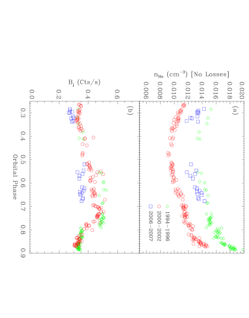
Figure 8: (a) Inferred He densities from a global fit to 238 He beam maps, with no correction for photoionization losses. The phase dependence is indicative of the presence of such losses. Different symbols are for different epochs, as in Figures 3–4. (b) Background count rates measured for the 238 maps in the global fit.

where $C^{\prime}_{j,i}=C^{\prime}_{j,i}[N_{j},B_{j},C_{j,i}(V_{ISM},\lambda,\beta,T)]$. Figure 8 shows the 238 $N_{j}$ and $B_{j}$ values that result from our best fit. The $B_{j}$ values are essentially identical to the backgrounds shown in Figure 4b, measured in the Gaussian fit analysis. The $N_{j}$ factors are directly related to inferred He densities (see above), so that is how they are shown in the figure. The clear phase dependence is an effect of photoionization losses, which are more severe at intermediate phases when the spacecraft is closer to the Sun. We will discuss this issue in detail in Section 5 when we actually seek to correct for photoionization.

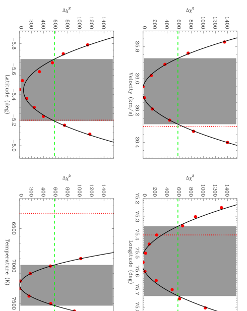
Figure 9: Helium flow parameter measurements from a global fit to the Ulysses/GAS data. In each panel, we plot $\Delta\chi^{2}$ as a function of one of the four He flow parameters of interest, where each point represents a separate fit with that parameter held constant and the other three parameters allowed to vary freely. Solid lines show polynomial fits to the data points. The horizontal dashed line corresponds to a $3\sigma$ contour, which we use to define our uncertainty range in each parameter (shaded regions). Vertical dotted lines are the Witte (2004) results, which are only significantly discrepant for the temperature.

We need to not only find the best fit but also to estimate uncertainties in the fit parameters, so the full analysis actually involves a series of fits with one of the four flow parameters held constant, as we scan through the parameters to see how $\chi^{2}$ varies with $V_{ISM}$, $\lambda$, $\beta$, and $T$. Results are shown in Figure 9. There is a very clear $\chi^{2}$ minimum, $\chi^{2}_{min}$, in each panel. We define $\Delta\chi^{2}\equiv\chi^{2}-\chi^{2}_{min}$, and each panel of Figure 9 shows the variation of $\Delta\chi^{2}$ across the $\chi^{2}_{min}$ region. Fifth order polynomials are fitted to the data points to interpolate between them. The $\Delta\chi^{2}$ values are used to define the error bounds around $\chi^{2}_{min}$. Bevington & Robinson (1992) and Press et al. (1989) both provide useful discussions about how best to do this. For the number of free parameters of our fit (480), the $3\sigma$ confidence contour corresponds to $\Delta\chi^{2}=578.3$, based on relation 26.4.14 of Abramowitz & Stegun (1965). This is the $\Delta\chi^{2}$ level used to define the uncertainty ranges shown in Figure 9.

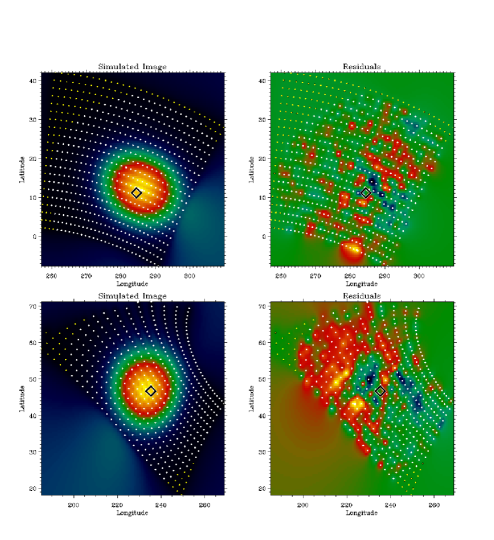
Figure 10: The top row shows a He beam map from 1994 November 9, a simulated map based on our best global fit to the Ulysses data, and the residuals of this fit. The bottom row is a similar set of images for a He beam map from 2007 November 26. The diamond indicates the expected beam position based on the Witte (2004) vector (assuming $T=0$ K). Yellow dots are scan positions, and white dots are the measurements within $25^{\circ}$ of the diamond, which are the data considered in the fit.

Our final derived He flow parameters are: $V_{ISM}=26.08\pm 0.21$ km s^-1, $\lambda=75.54\pm 0.19$ deg, $\beta=-5.44\pm 0.24$ deg, and $T=7260\pm 270$ K; which are listed in the first line of Table 1. Our best global fit has $\chi^{2}_{\nu}=1.524$, which is somewhat higher than it should be ideally, indicating a modest level of systematic discrepancy from the data. It is not practical to show the actual fit to the data for all 238 beam maps, but for illustrative purposes Figure 10 shows the fit for two particular maps, one from 1994 November 9 and another from 2007 November 26. The former exhibits no clear systematic deviation between the fit and the data, but the latter shows some systematic deviation.

Calculations involving photoionization will be discussed in more detail in Section 5, but at this point we mention that in order to see whether photoionization could be affecting our He vector and T measurements, we tried redoing the global fit assuming a He photoionization rate at 1 AU of $\beta_{ion}=1.5\times 10^{-7}$ s^-1, which is near the high end of those typically estimated (Bzowski et al., 2012; Katushkina et al., 2014). The resulting parameters and $\chi^{2}$ are: $V_{ISM}=26.11\pm 0.21$ km s^-1, $\lambda=75.47\pm 0.18$ deg, $\beta=-5.49\pm 0.23$ deg, $T=7330\pm 280$ K, $\chi^{2}_{\nu}=1.528$. These values are very similar to those found before, so considering photoionization does not change the derived vector or temperature significantly, and does not affect the quality of fit, consistent with the findings of Katushkina et al. (2014).

Figure 9 and Table 1 demonstrate that our results are generally in very good agreement with the previous canonical Ulysses measurements from Witte (2004), with the exception of $T$. Our temperature is significantly higher than the $T=6300\pm 340$ K measurement of Witte (2004). As discussed in Section 2, we are working with a new reduction of the Ulysses data, but we have performed fits to He beam maps from the older data reduction, and we do not find any significant effect on our derived temperature. We initially suspected that our higher $T$ measurement may be an artifact of the global fitting approach. To first order, $T$ is determined mostly by the size of the observed He beams, while the other three parameters determine its direction. If the global fit has difficulty simultaneously reproducing the beam center for all 238 beam maps, it will try to compromise by broadening the beam, increasing the inferred $T$. This effect will not be an issue with single-map fits, and so would not affect the Witte (2004) analysis approach.

We perform single-map fits to our 238 beam maps, where we fix $V_{ISM}=26.08$ km s^-1 in order to resolve the parameter degeneracy problem with single-map fits described above. This provides 238 measurements of $\lambda$, $\beta$, and $T$. The average and standard deviation of these values are reported in the second line of Table 1. The $\lambda$ and $\beta$ measurements are nearly identical to the global fit values. The $T=7090\pm 370$ K measurement is somewhat lower than the $T=7260\pm 270$ K global fit value, as expected, but not by that much. Experimenting with other velocity values within our quoted $V_{ISM}=26.08\pm 0.21$ km s^-1 range does not change things significantly. We conclude that the beam-broadening effect of the global fit is not the dominant cause of our higher $T$.

Differences in background treatment are another possible cause of the $T$ discrepancy. The original Ulysses data analyses excluded pixels with count rates too close to the background value (Banaszkiewicz et al., 1996). Typically only the upper $\sim 80$% of the profile was considered, whereas our approach is to consider all pixels within $25^{\circ}$ of the beam, with the background determination actually being part of the fit rather than assuming a predetermined background. We have considered the possibility that focusing more on the central part of the beam could lead to the perception of a narrower beam and therefore a lower $T$. However, using single-map fits we have investigated the effects of focusing on the central part of the beam and we do not find that such fits consistently lead to significantly lower temperatures. Thus, we ultimately dismiss this possible explanation for our high $T$ measurement.

We note that our higher temperature is in better agreement with the $T=7500\pm 1300$ K Local Interstellar Cloud (LIC) temperature estimated from ISM absorption lines (Redfield & Linsky, 2008). It is also consistent with another contemporaneous reassessment of the Ulysses He data by Bzowski et al. (2014), largely following the same analysis approach used previously to study IBEX data (Bzowski et al., 2012). Their derived best-fit He flow parameters ($V_{ISM}=26.0$ km s^-1, $\lambda=75.3^{\circ}$, $\beta=-6^{\circ}$, $T=7500$ K) are in reasonably good agreement with our results, including the higher temperature.

The only difference is that Bzowski et al. (2014) claim much larger uncertainties. Specifically, the parameters are quoted as having uncertainty ranges of $74.2^{\circ}<\lambda<76.5^{\circ}$, $-7^{\circ}<\beta<-5^{\circ}$, $24.5<V_{ISM}<27.0$ km s^-1, and $5500<T<9000$ K. The large error bars are based on independent analyses of data taken from different parts of the Ulysses orbit, but we consider these error bars to be overly conservative, as this analysis approach greatly weakens the diagnostic power of considering data from all parts of the Ulysses orbit simultaneously, which is crucial to the efficacy of the global fit approach. Figure 7 indicates how $\lambda$, $\beta$, and $V_{ISM}$ change the shape of the horseshoe-shaped track for the He beam in different ways, and it is this effect that allows the global fit approach to break the degeneracies that plague single-map analyses (see Figure 6). Considering observations from only one part of the Ulysses orbit will in effect reintroduce the degeneracy problem, naturally leading to the inference of the large uncertainties quoted by Bzowski et al. (2014). To put it another way, we see the large uncertainties quoted by Bzowski et al. (2014) as being a further demonstration of the importance of considering data from all parts of the Ulysses orbit together, rather than being an accurate quantification of systematic uncertainties inherent in these data.

The cause of the higher T inferred both by ourselves and Bzowski et al. (2014) remains to be explained. Having excluded the possibilities mentioned above, we conclude that the most likely cause of this discrepancy with Witte (2004) lies in the Bayesian statistics of the older analyses. While our analysis and that of Bzowski et al. (2014) rely solely on the $\chi^{2}$ statistic to quantify how well a set of parameters is fitting the data, the older analyses instead use a Bayesian merit function that considers not only consistency with the data, but also consistency with prior assumptions about what the best-fit parameters should be (see eqn. 10 from Banaszkiewicz et al., 1996). The advantage of this Bayesian approach is that this is one way to break the degeneracies in single-map fits, and derive relatively self-consistent single-map measurements like those shown in Figure 2 of Witte (2004). The disadvantage is that the analysis is potentially biased by the a priori assumption of expected best-fit parameters, as well as the question of how to weight the relative importance of consistency with those parameters and consistency with the data. The clearest distinction between our analysis and the older ones lies in this difference in how the best fit is defined, so we propose that the Bayesian approach of the older work drove the analysis towards a lower temperature, while the pure $\chi^{2}$-minimization analysis used here and by Bzowski et al. (2014) leads to a higher temperature.

The higher temperature suggested by both our analysis and that of Bzowski et al. (2014) could have relevance for the discrepancy in the IBEX and Ulysses He flow vectors. The IBEX analysis suffers from the same kind of parameter degeneracies discussed above for Ulysses. Although the IBEX data suggest a $\chi^{2}$ minimum for $T\approx 6200$ K (Bzowski et al., 2012), it is not clear that significantly higher temperatures are excluded by the data. Furthermore, the parameter dependencies for IBEX are such that assuming a higher temperature would push the IBEX-derived $\lambda$ and $V_{ISM}$ values closer to those of Ulysses. Specifically, assuming our $T=7260\pm 270$ K measurement would yield the following values from IBEX: $\lambda=77.1\pm 0.5^{\circ}$ and $V_{ISM}=24.6\pm 0.4$ km s^-1 (Bzowski et al., 2012; Möbius et al., 2012; McComas et al., 2012). These values are still not quite consistent with Ulysses, but they are significantly closer than the McComas et al. (2012) values quoted in Section 1.

A likely important source of systematic uncertainty in the Ulysses data analysis that we want to emphasize is uncertainty in the detection efficiency ($D_{e}$) curve in Figure 5b. It is important to note that He atoms are typically detected in the $E_{s}=30-60$ eV range. This is very much in the “knee” of the $D_{e}$ curve, where $D_{e}$ is significantly energy dependent. Combine this energy dependence with the fact that there is generally a significant gradient of average particle energy across a He beam, and the result is a situation where particle detection efficiency is higher on one side of the beam than the other, leading to an observed beam that is shifted from where one might naively expect to see it. This is clearly the case in Figure 6 for example, where the observed beam is shifted to the left from its expected location based on a zero-temperature calculation assuming the Witte (2004) vector.

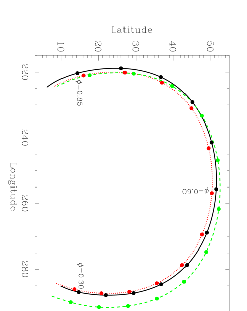
Figure 11: The solid line is the observed track of the He beam center during the Ulysses orbit, from Figure 3a, which is compared with the expected beam center based on our best-fit He flow vector (dotted line) and the IBEX-derived flow vector (dashed line) from McComas et al. (2012). The expected beam centers are computed assuming $T=0$ K, and the difference between the best-fit and observed tracks indicates the level of uncertainty introduced by that assumption (see text). Dots mark orbital phases between $\phi=0.30$ and $\phi=0.85$ in increments of $\Delta\phi=0.05$.

This effect is shown in more detail in Figure 11, which compares the observed trace of the He beam center from Figure 3a with a trace computed from our best-fit He flow vector, assuming $T=0$ K. The average discrepancy between these two horseshoe-shaped tracks is $1.40^{\circ}$, which is at least mostly due to the effects of $D_{e}$ described above. The magnitude of this effect will be quite sensitive to the slope of the $D_{e}$ curve around $E_{s}=45$ eV. We therefore suspect that uncertainties in this slope are an important source of systematic error in the Ulysses analysis.

Could this effect in principle resolve the discrepancy in the IBEX and Ulysses He flow vectors? To investigate this possibility, Figure 11 shows the location of the horseshoe track that Ulysses should have observed if the IBEX vector of McComas et al. (2012) was correct, approximated once again with the $T=0$ K assumption. In most places along the horseshoe, the $D_{e}$ slope effect is not shifting the track towards the IBEX track, so assuming $D_{e}$ curves with different slopes will unfortunately not resolve the IBEX/Ulysses discrepancy. The IBEX track in Figure 11 is an average of $3.73^{\circ}$ from the observed track, illustrating the magnitude of the disagreement in angular terms. Based on Figure 7, the lower $V_{ISM}$ and higher $\lambda$ values measured by IBEX (see Section 1) would be expected to produce a horseshoe track that is broader and shifted to the right from that observed by Ulysses, and Figure 11 shows that explicitly.

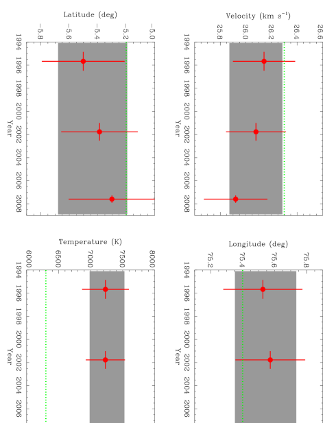
Figure 12: Helium flow parameter measurements from global fits to Ulysses/GAS data from the three fast latitude scans in 1994–1996, 2000–2002, and 2006–2007. The shaded regions correspond to the error bars defined in Figure 9. The horizontal dotted lines are the Witte (2004) parameters. We see no evidence for any He flow parameter variability from 1994–2007.

Finally, we revisit the issue of He flow variability by performing global fits to the Ulysses data separately for the three fast latitude scans, leading to independent measurements for 1994–1996, 2000–2002, and 2006–2007. Results are listed in Table 1 and displayed in Figure 12. Consistent with the findings of the empirical analysis of Section 3, we see no evidence for any He flow parameter variability, with the He flow direction varying by no more than $\sim 0.3^{\circ}$ from 1994–2007, and the velocity varying by no more than $\sim 0.3$ km s^-1. With IBEX data acquisition beginning in early 2009, there is less than a two year time gap for the $3.5^{\circ}$ jump in flow longitude to occur, if the variable flow interpretation of the IBEX/Ulysses discrepancy is correct (Frisch et al., 2013).

5 DENSITY AND PHOTOIONIZATION

The previous section described how we measured four of the five parameters describing the assumed Maxwellian He distribution in the ISM. The remaining parameter is the density, $n_{\rm He}$. Unlike the other four parameters, the density is significantly affected by loss processes that occur during the He atoms’ journey from the ISM to Ulysses. Thus, measuring $n_{\rm He}$ is somewhat more complicated. The loss rate, $\beta_{ion}({\rm r})$, is assumed to vary as $r^{-2}$, and is generally quantified by quoting the loss rate at 1 AU. For He, the most dominant loss process is photoionization by solar EUV photons, though electron impact ionization may also be non-negligible (Witte, 2004; Bzowski et al., 2013). For an assumed $\beta_{ion}$ at 1 AU, our particle tracking code can account for losses along the track, assuming the $r^{-2}$ dependence. At the ISM flow speed it takes about 500 days to travel from 10 AU inward to the observer (see, e.g., Figure 3 in Witte 2004), so the effective ionization rate should be an average of the rates encountered over the past year or so, weighted as $r^{-2}$.

The usual procedure for dealing with photoionization is to rely on estimates of $\beta_{ion}$ from various monitors of solar EUV emission (McMullin et al., 2004; Auchère et al., 2005; Woods et al., 2005; Lean et al., 2011; Bzowski et al., 2013). However, this process carries significant uncertainties, as many of the EUV irradiance proxies are less than ideal for our purposes, and some of them are inconsistent. The Solar EUV Experiment (SEE) on the Thermospheric Ionospheric Mesospheric Energy and Dynamics (TIMED) spacecraft has significantly improved matters, but it was launched in 2002, and so does not cover most of the Ulysses time period. Lean et al. (2011) quote uncertainties in EUV irradiance of 10%-20% in the SEE era, but up to a factor of 2 uncertainties before it. The SEE EUV measurements have been correlated with other solar activity indicators that have been monitored for many decades (e.g., Mg II, $F_{10.7}$), allowing those indicators to be utilized as EUV proxies. This has improved matters even for the older time period.

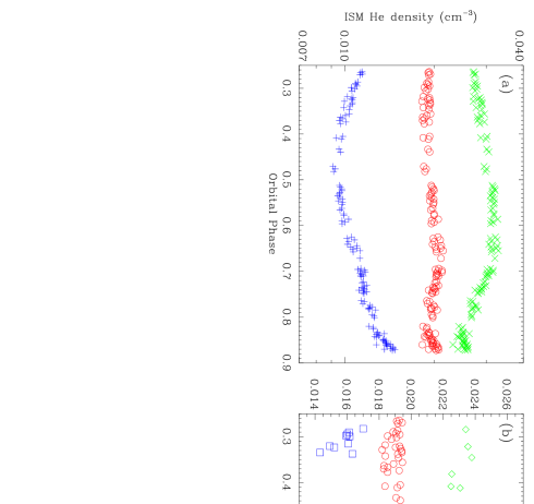
Figure 13: (a) Interstellar He densities computed from the second fast latitude scan (2000–2002), plotted versus orbital phase, assuming photoionization loss rates of $\beta_{ion}=0$ s^-1 (plus signs), $1.79\times 10^{-7}$ s^-1 (circles), and $3.0\times 10^{-7}$ (X’s) s^-1. The $\beta_{ion}=1.79\times 10^{-7}$ s^-1 case is where the variability of the densities is minimized. (b) Inferred He densities plotted as a function of orbital phase for the first (diamonds), second (circles), and third (squares) fast latitude scans. For each of the three sets of measurements the loss rate is chosen to minimize variability in density with orbital phase. These rates are $1.36\times 10^{-7}$, $1.79\times 10^{-7}$, and $5.7\times 10^{-8}$ s^-1 for scans one, two, and three, respectively.

Nevertheless, we here try a different technique for dealing with photoionization that uses only Ulysses constraints. Focusing on the second fast latitude scan (2000–2002), Figure 13a shows densities measured as a function of orbital phase, computed assuming different photoionization rates. When an overly low rate is assumed ($\beta_{ion}=0$ s^-1 in the figure) the result is a U-shaped curve with low densities at intermediate phases ($\phi=0.4-0.6$). Although densities at all phases will be underestimates, the effect is more pronounced at these intermediate phases, since that is when Ulysses is closest to the Sun and therefore observes a He flow with the highest losses. Conversely, when an overly high rate is assumed ($\beta_{ion}=3.0\times 10^{-7}$ s^-1 in the figure) the pattern reverses and overly high densities are observed at intermediate phases, indicative of an overcompensation in the loss correction.

We define the most likely photoionization loss rate as that which leads to the flattest density-vs-phase curve. Specifically, we compute the standard deviation of the density measurements divided by the average density, $\sigma_{n}(\beta_{ion})/\bar{n}(\beta_{ion})$, and we find the $\beta_{ion}$ value that minimizes this quantity. At this minimum, the average density $\bar{n}$ is then our $n_{\rm He}$ measurement, and the minimum deviation is $\sigma_{n,min}/n_{\rm He}$. We estimate 1$\sigma$ uncertainties for our loss rate and density measurements using the standard deviation of the mean at this minimum, $\sigma_{mean}=\sigma_{n,min}/\sqrt{N_{m}}$, where here $N_{m}$ is the number of measurements. The range of acceptable loss rates are then defined to be where

$$\frac{\sigma_{n}(\beta_{ion})}{\bar{n}(\beta_{ion})}<\frac{\sigma_{n,min}+\sigma_{mean}}{n_{\rm He}}.$$ (5)

For the epoch 2 data in Figure 13a, the minimum density variance is at $\beta_{ion}=1.79\times 10^{-7}$ s^-1, and the resulting densities are shown in the figure. Assuming this rate, the average He density is then computed to be $n_{\rm He}=0.0197$ cm^-3. Figure 13b displays the density measurements for all three epochs. The inferred densities and photoionization rates are listed in Table 2, along with the $1\sigma$ uncertainties computed as described above. For epoch 3, the analysis is less constrained due to fewer data points and intrinsically greater scatter (see Figure 13b), so we essentially find only an upper limit to $\beta_{ion}$.

The densities independently measured from the three epochs are not identical. Assuming that the ISM He density does not really vary, the degree of inconsistency is presumably an indication of the uncertainties in the loss correction, although detector sensitivity uncertainties are also a potential factor. The stability of the detector sensitivity was tested twice during the course of the mission. New layers of LiF were evaporated onto the surface from the GAS instrument’s LiF supply in 1995 and 2001. The He signal was measured immediately before and after each deposition. It showed that the detection efficiency did not change within the available statistical accuracy of 20%. Unfortunately, a third test planned for 2006 had to be cancelled, as the power necessary to heat the LiF supply may have exceeded the power available to the spacecraft at the time, which had decreased during the course of the mission. Thus, it cannot be proven that the detection efficency did not degrade during the third and final epoch, altough it seems unlikely in view of past experience. In any case, the average and standard deviation of the three measurements in Table 2 provides our final best estimate for the ISM He density: $n_{\rm He}=0.0196\pm 0.0033$ cm^-3. This is somewhat higher than the $n_{\rm He}=0.015\pm 0.003$ cm^-3 measurement from Witte (2004), due at least in part to higher assumed photoionization rates, but the error bars overlap.

Table 2 compares our inferred loss rates with average ones estimated by Bzowski et al. (2013, 2014) for the three epochs based on solar wind and EUV constraints, taking into consideration both photoionization and electron impact ionization. There is actually good agreement for epochs 2 and 3, but not for epoch 1, where our $\beta_{ion}=(1.36\pm 0.27)\times 10^{-7}$ s^-1 is significantly higher than the $\beta_{ion}=0.9\times 10^{-7}$ s^-1 rate expected for this period. Given that our estimated density is also rather high, it seems likely that our analysis approach has led to an overestimate of $\beta_{ion}$. Our technique of minimizing phase-dependent density variation does have the drawback of not accounting for any change in photoionization rate that might occur in the 20 month period covering the $\phi=0.25-0.90$ fast-latitude scan range. However, the loss rates estimated by Bzowski et al. (2013, 2014) do not actually show much variation during epoch 1, so unidentified issues may also be present.

6 SUMMARY

Motivated in part by the discrepancy in the He flow vectors measured by Ulysses and IBEX, we have performed an independent analysis of the Ulysses/GAS data set from 1994-2007, newly reprocessed in 2013, including 2006–2007 data not included in the canonical Witte (2004) analysis. Our findings are summarized as follows:

1.

We first perform a purely empirical analysis of the He beam observed by Ulysses, using 2-D Gaussian fits to quantify beam location, amplitude, and width; in order to see how these parameters vary with orbital phase and time. There is no evidence for intrinsic variability in beam direction by more than a few tenths of a degree. The beam widths are also invariant within measurement uncertainties.

2.

The lack of variability in the He beam from 1994–2007 makes it harder to explain the IBEX/Ulysses discrepancy in terms of He flow variability, with less than a two-year time gap for that change in flow to occur before IBEX observations begin in 2009.

3.

We demonstrate that the most powerful constraint that the Ulysses/GAS data provide on the He flow vector lies in the shape of the horseshoe-shaped track made by the He beam over the course of a Ulysses orbit, which breaks parameter degeneracies that plague attempts to derive He flow parameters from individual beam maps. Only by fitting the Ulysses/GAS data collectively can this diagnostic power be fully utilized.

4.

From a global fit to the full Ulysses/GAS data set from 1994–2007, we find the following He flow parameters: $V_{ISM}=26.08\pm 0.21$ km s^-1, $\lambda=75.54\pm 0.19^{\circ}$, $\beta=-5.44\pm 0.24^{\circ}$, and $T=7260\pm 270$ K. Separate global fits to the three separate fast-latitude scans confirm a lack of He flow parameter variability, with the flow direction varying by no more than $\sim 0.3^{\circ}$ and the velocity by no more than $\sim 0.3$ km s^-1.

5.

Our ($V_{ISM}$,$\lambda$,$\beta$) He vector is consistent with the previous canonical measurements of Witte (2004) and the contemporaneous analysis of Bzowski et al. (2014), proving that the IBEX/Ulysses discrepancy is not a product of different analysis approaches. The cause of the IBEX/Ulysses discrepancy remains unknown.

6.

Our temperature measurement ($T=7260\pm 270$ K) is somewhat higher than the $T=6300\pm 340$ K value of Witte (2004), but is consistent with the $T=7500$ K best-fit value of Bzowski et al. (2014), although Bzowski et al. (2014) quote a much larger range of acceptable values ($5500<T<9000$ K). A higher temperature potentially mitigates the IBEX/Ulysses discrepancy somewhat, as the parameter dependencies in the IBEX analysis are such that a higher $T$ would lead to lower $\lambda$ and higher $V_{ISM}$, moving the IBEX-derived values closer to those of Ulysses.

7.

Using a technique to infer photoionization loss rates solely from Ulysses constraints, we compute He densities and loss rates for the three epochs of observation (1994–1996, 2000–2002, and 2006–2007). Our loss rates agree well with expectations from solar EUV constraints for epochs 2 and 3, but not for epoch 1, where we seem to overestimate the rate. Our final density measurement is $n_{\rm He}=0.0196\pm 0.0033$ cm^-3, somewhat higher than estimated by Witte (2004), $n_{\rm He}=0.015\pm 0.003$ cm^-3.

Table 1: Ulysses Measurements of the ISM He Flow

Years	Fit Type	$V_{ISM}$	$\lambda$ (J2000)	$\beta$ (J2000)	T	Source
		(km s-1)	(deg)	(deg)	(K)
1994–2007	Global Fit	$26.08\pm 0.21$	$75.54\pm 0.19$	$-5.44\pm 0.24$	$7260\pm 270$	this work
1994–2007	Single Maps	(26.08)	$75.60\pm 0.34$	$-5.38\pm 0.37$	$7090\pm 370$	this work
1994–1996	Global Fit	$26.14\pm 0.24$	$75.53\pm 0.25$	$-5.50\pm 0.29$	$7230\pm 360$	this work
2000–2002	Global Fit	$26.08\pm 0.23$	$75.57\pm 0.22$	$-5.39\pm 0.27$	$7230\pm 310$	this work
2006–2007	Global Fit	$25.92\pm 0.25$	$75.42\pm 0.17$	$-5.30\pm 0.30$	$7270\pm 220$	this work
1990–2002	Single Maps	$26.3\pm 0.4$	$75.4\pm 0.5$	$-5.2\pm 0.2$	$6300\pm 340$	Witte (2004)

Table 2: Density and Photoionization

Years	$n_{\rm He}$ from Fit	$\beta_{ion}$ from Fit	$\beta_{ion}$ from EUV
	($10^{-2}$ cm-3)	($10^{-7}$ s-1)	($10^{-7}$ s-1)
1994–1996	$2.28\pm 0.14$	$1.36\pm 0.27$	0.9
2000–2002	$1.97\pm 0.18$	$1.79\pm 0.31$	1.6
2006–2007	$1.62^{+0.58}_{-0.31}$	$0.57^{+0.92}_{-0.57}$	0.7

Figure 2: The left panel is a WFOV helium beam map from 2001 July 6, in ecliptic coordinates, the middle panel is a 2-D Gaussian fit to the He peak, and the right panel shows the residuals of the fit. The count rates shown are in cts s^-1 pixel^-1.

Figure 5: (a) Detector geometry function for the WFOV (solid line) and NFOV (dotted line) detectors. (b) Detection efficiency as a function of incoming particle energy.

References

- Abramowitz & Stegun (1965) Abramowitz, M., & Stegun, I. A. 1965, Handbook of Mathematical Functions (New York: Dover Publications, Inc.)
- Auchère et al. (2005) Auchère, F., Cook, J. W., Newmark, J. S., McMullin, D. R., von Steiger, R., & Witte, M. 2005, ApJ, 625, 1036
- Banaszkiewicz et al. (1996) Banaszkiewicz, M., Witte, M., & Rosenbauer, H. 1996, A&AS, 120, 587
- Ben-Jaffel et al. (2013) Ben-Jaffel, L., Strumik, M., Ratkiewicz, R., & Grygorczuk, J. 2013, ApJ, 779, 130
- Bevington & Robinson (1992) Bevington, P. R., & Robinson, D. K. 1992, Data Reduction and Error Analysis for the Physical Sciences (New York: McGraw-Hill)
- Bzowski et al. (2012) Bzowski, M., et al. 2012, ApJS, 198, 12
- Bzowski et al. (2013) Bzowski, M., Sokół, J. M., Kubiak, M. A., & Kucharek, H. 2013, A&A, 557, A50
- Bzowski et al. (2014) Bzowski, M., Kubiak, M. A., Hłond, M., Sokół, J. M., Banaszkiewicz, M., & Witte, M. 2014, A&A, submitted (http://arxiv.org/abs/1405.0623)
- Frisch et al. (2013) Frisch, P. C., et al. 2013, Science, 341, 1080
- Gry & Jenkins (2014) Gry, C., & Jenkins, E. B. 2014, A&A, 567, A58
- Katushkina et al. (2014) Katushkina, O. A., Izmodenov, V. V., Wood, B. E., & McMullin, D. R. 2014, ApJ, in press
- Lallement & Bertaux (2014) Lallement, R., & Bertaux, J. L. 2014, A&A, 565, A41
- Lallement & Bertin (1992) Lallement, R., & Bertin, P. 1992, A&A, 266, 479
- Lean et al. (2011) Lean, J. L., Woods, T. N., Eparvier, F. G., Meier, R. R., Strickland, D. J., Correira, J. T., & Evans, J. S. 2011, J. Geophys. Res., 116, A01102
- Marsden (2001) Marsden, R. G. 2001, Ap&SS, 277, 337
- McComas et al. (2012) McComas, D. J., et al. 2012, Science, 336, 1291
- McMullin et al. (2004) McMullin, D. R., et al. 2004, A&A, 426, 885
- Möbius et al. (2012) Möbius, E., et al. 2012, ApJS, 198, 11
- Müller (2012) Müller, H. -R. 2012, in Numerical Modeling of Space Plasma Flows (Astronum 2011), ed. N. V. Pogorelov, et al. (San Francisco: ASP, Vol. 459), 228 (http://arxiv.org/abs/1205.1555)
- Müller et al. (2013) Müller, H. -R., Bzowski, M., Möbius, E., & Zank, G. P. 2013, in Solar Wind 13, ed. G. P. Zank, et al. (New York: AIP, Vol. 1539), 348
- Müller & Cohen (2012) Müller, H. -R., & Cohen, J. H. 2012, in Physics of the Heliosphere: A 10-year Retrospective, ed. J. Heerikhuisen & G. Li, (AIP Vol. 1436), 233 (http://arxiv.org/abs/1205.0967)
- Press et al. (1989) Press, W. H., Flannery, B. P., Teukolsky, S. A., & Vetterling, W. T. 1989, Numerical Recipes (Cambridge: Cambridge University Press)
- Redfield & Linsky (2008) Redfield, S., & Linsky, J. L. 2008, ApJ, 673, 283
- Scherer & Fichtner (2014) Scherer, K., & Fichtner, H. 2014, ApJ, 782, 25
- Vincent et al. (2014) Vincent, F. E., et al. 2014, ApJ, 788, L25
- Wenzel et al. (1992) Wenzel, K. P., Marsden, R. G., Page, D. E., & Smith, E. J. 1992, A&AS, 92, 207
- Witte (2004) Witte, M. 2004, A&A, 426, 835
- Witte et al. (1996) Witte, M., Banaszkiewicz, M., & Rosenbauer, H. 1996, Space Sci. Rev., 78, 289
- Witte et al. (1993) Witte, M., Rosenbauer, H., Banaszkiewicz, M., & Fahr, H. 1993, Adv. Space Res., 13, 121
- Witte et al. (1992) Witte, M., Rosenbauer, H., Keppler, E., Fahr, H., Hemmerich, P., Lauche, H., Loidl, A., & Zwick, R. 1992, A&AS, 92, 333
- Woods et al. (2005) Woods, T. N., et al. 2005, J. Geophys. Res., 110, A01312
- Zank et al. (2013) Zank, G. P., Heerikhuisen, J., Wood, B. E., Pogorelov, N. V., Zirnstein, E., & McComas, D. J. 2013, ApJ, 763, 20
- Zieger et al. (2013) Zieger, B., Opher, M., Schwadron, N. A., McComas, D. J., & Tóth, G. 2013, Geophys. Res. Lett., 40, 2923