Quantum effects on Lagrangian points and displaced periodic orbits in the Earth-Moon system

Abstract

Recent work in the literature has shown that the one-loop long distance quantum corrections to the Newtonian potential imply tiny but observable effects in the restricted three-body problem of celestial mechanics, i.e., at the Lagrangian libration points of stable equilibrium the planetoid is not exactly at equal distance from the two bodies of large mass, but the Newtonian values of its coordinates are changed by a few millimeters in the Earth-Moon system. First, we assess such a theoretical calculation by exploiting the full theory of the quintic equation, i.e., its reduction to Bring-Jerrard form and the resulting expression of roots in terms of generalized hypergeometric functions. By performing the numerical analysis of the exact formulas for the roots, we confirm and slightly improve the theoretical evaluation of quantum corrected coordinates of Lagrangian libration points of stable equilibrium. Second, we prove in detail that also for collinear Lagrangian points the quantum corrections are of the same order of magnitude in the Earth-Moon system. Third, we discuss the prospects to measure, with the help of laser ranging, the above departure from the equilateral triangle picture, which is a challenging task. On the other hand, a modern version of the planetoid is the solar sail, and much progress has been made, in recent years, on the displaced periodic orbits of solar sails at all libration points, both stable and unstable. The present paper investigates therefore, eventually, a restricted three-body problem involving Earth, Moon and a solar sail. By taking into account the one-loop quantum corrections to the Newtonian potential, displaced periodic orbits of the solar sail at libration points are again found to exist.

I Introduction

From the point of view of modern theoretical physics, the logical need for a quantum theory of gravity is suggested by the Einstein equations themselves, which tell us that gravity couples to $T_{\mu\nu}$, the energy-momentum tensor of matter, in a diffeomorphism-invariant way, by virtue of the tensor equations Einstein1916 ; Bruhat09

$$R_{\mu\nu}-{1\over 2}g_{\mu\nu}R={8\pi G\over c^{4}}T_{\mu\nu}.$$ (1)

When Einstein arrived at these equations, although he had already understood that the classical Maxwell theory of electromagnetic phenomena is not valid in all circumstances, the only known forms of $T_{\mu\nu}$ were classical, e.g., the energy-momentum tensor of a relativistic fluid, or even just the case of vacuum Einstein equations, for which $T_{\mu\nu}$ vanishes. In due course, it was realized that matter fields are quantum fields in the first place (e.g., a massive Dirac field, or spinor electrodynamics). The quantum fields are operator-valued distributions Wightman96 , for which a regularization and renormalization procedure is necessary and even fruitful. However, the mere replacement of $T_{\mu\nu}$ by its regularized and renormalized form $\langle T_{\mu\nu}\rangle$ on the right-hand side of Eq. (1.1) leads to a hybrid scheme, because the classical Einstein tensor $R_{\mu\nu}-{1\over 2}g_{\mu\nu}R$ is affected by the coupling to $\langle T_{\mu\nu}\rangle$. The question then arises whether the appropriate, full quantum theory of gravity should have field-theoretical nature or should involve, instead, other structures (e.g., strings Polchinski98 or loops Rovelli04 or twistors Penrose73 ), and at least $16$ respectable approaches Espo11 have been developed so far in the literature. To make such theories truly physical, their predictions should be checked against observations. For example, applications of the covariant theory lead to detailed predictions for the cross sections of various scattering processes DeWitt1967c , but such phenomena (if any) occur at energy scales inaccessible to observations, and also the effects of Planck-scale physics on cosmology, e.g., the cosmic microwave background radiation and its anisotropy spectrum Kiefer12 ; Bini13 ; Bini14 ; Kamen13 ; Kamen14 , are not yet easily accessible to observations, although cosmology offers possibly the best chances for testing quantum gravity Wilczek14 .

Recently, inspired by the work in Refs. D94 ; D94b ; D94c ; MV95 ; HL95 ; ABS97 ; KK02 ; D03 on effective field theories of gravity, where it is shown that the leading (i.e., one-loop) long distance quantum corrections to the Newtonian potential are entirely ruled by the Einstein-Hilbert part of the full action functional, some of us BE14a ; BE14b have assumed that such a theoretical analysis can be applied to the long distances and macroscopic bodies occurring in celestial mechanics P1890 ; P1892 ; Pars65 . More precisely, the Newtonian potential between two bodies of masses $m_{A}$ and $m_{B}$ receives quantum corrections leading to D03

$$V_{Q}(r)=-{Gm_{A}m_{B}\over r}\left(1+{k_{1}\over r}+{k_{2}\over r^{2}}\right)+{\rm O}(G^{2}),$$ (2)

where BE14a

$$k_{1}\equiv\kappa_{1}{G(m_{A}+m_{B})\over c^{2}},$$ (3)

$$k_{2}\equiv\kappa_{2}{G\hbar\over c^{3}}=\kappa_{2}(l_{P})^{2}.$$ (4)

Equation (1.2) implies that, $\forall\varepsilon>0$, there exists an $r_{0}$ value of $r$ such that

$$\left|V_{Q}(r)+{Gm_{A}m_{B}\over r}\left(1+{k_{1}\over r}+{k_{2}\over r^{2}}\right)\right|<\varepsilon,\;\forall r>r_{0}.$$ (5)

This feature will play an important role in our concluding remarks in Sec. V.

We also stress that the dimensionless parameter $\kappa_{1}$ depends on the dimensionless parameter $\kappa_{2}$. In other words, $k_{1}$ is a post-Newtonian term which only depends on classical physical constants, but its weight, expressed by the real number $\kappa_{1}$, is affected by the calculational procedure leading to the fully quantum term $k_{2}$, where the real number $\kappa_{2}$ weighs the Planck length squared. More precisely, the perturbative expansion involves only integer powers of Newton’s constant G:

$$V_{Q}(r)\sim-{Gm_{A}m_{B}\over r}\left(1+\sum_{p=1}^{\infty}f_{p}(r)G^{p}\right)\sim-{Gm_{A}m_{B}\over r}\left(1+\sum_{n=1}^{\infty}{k_{n}\over r^{n}}\right),$$ (6)

where, upon denoting by $L_{A}$ and $L_{B}$ the gravitational radii $L_{A}\equiv{Gm_{A}\over c^{2}},L_{B}\equiv{Gm_{B}\over c^{2}}$, one has the coefficients $k_{n}=k_{n}(L_{A}+L_{B},(l_{P})^{2})$. At one loop, i.e., to linear order in $G$, where

$$f_{1}(r)=\kappa_{1}{(m_{A}+m_{B})\over c^{2}}{1\over r}+\kappa_{2}{\hbar\over c^{3}}{1\over r^{2}},$$ (7)

we can only have the contribution ${(L_{A}+L_{B})\over r}$ with weight equal to the real number $\kappa_{1}$, and the contribution ${(l_{P})^{2}\over r^{2}}$ with weight equal to the real number $\kappa_{2}$. Although the term ${(l_{P})^{2}\over r^{2}}$ is overwhelmed by the term ${(L_{A}+L_{B})\over r}$, the two are inextricably intertwined because $\kappa_{1}$ is not a free real parameter but depends on $\kappa_{2}$: both $\kappa_{1}$ and $\kappa_{2}$ result from loop diagrams. Thus, the one-loop long distance quantum correction is the whole term

$$f_{1}(r)G={k_{1}\over r}+{k_{2}\over r^{2}}=\kappa_{1}{(L_{A}+L_{B})\over r}+\kappa_{2}{(l_{P})^{2}\over r^{2}},$$ (8)

where $\kappa_{1}$ takes a certain value because there exists a nonvanishing value of $\kappa_{2}$. The authors of Ref. D03 found the numerical values

$$\kappa_{1}=3,\;\kappa_{2}={41\over 10\pi}.$$ (9)

The work in Ref. BE14a considered the application of Eqs. (1.2)-(1.4) and (1.9) to the circular restricted three-body problem of celestial mechanics, in which two bodies $A$ and $B$ of masses $\alpha$ and $\beta$, respectively, with $\alpha>\beta$, move in such a way that the orbit of $B$ relative to $A$ is circular, and hence both $A$ and $B$ move along circular orbits around their center of mass $C$ which moves in a straight line or is at rest, while a third body, the planetoid $P$, of mass $m$ much smaller than $\alpha$ and $\beta$, is subject to their gravitational attraction, and one wants to evaluate the motion of the planetoid. On taking rotating axes with center of mass $C$ as origin, distance $AB$ denoted by $l$, and angular velocity $\omega$ given by

$$\omega=\sqrt{G(\alpha+\beta)\over l^{3}},$$ (10)

one has, with the notation in Fig. 1, that the quantum corrected effective potential for the circular restricted three-body problem is given by $GU$, where BE14a

$$U={1\over 2}{(\alpha+\beta)\over l^{3}}(x^{2}+y^{2})+{\alpha\over r}\left(1+{k_{1}\over r}+{k_{2}\over r^{2}}\right)+{\beta\over s}\left(1+{k_{3}\over s}+{k_{2}\over s^{2}}\right),$$ (11)

where $r$ and $s$ are the distances $AP$ and $BP$, respectively, while here

$$k_{1}\equiv\kappa_{1}{G(m+\alpha)\over c^{2}},\;k_{3}\equiv\kappa_{3}{G(m+\beta)\over c^{2}},\kappa_{1}=\kappa_{3}=3.$$ (12)

The equilibrium points are found by studying the gradient of $U$ and evaluating its zeros. There exist indeed five zeros of ${\rm grad}U$ BE14a . Three of them correspond to collinear libration points $L_{1},L_{2},L_{3}$ of unstable equilibrium, while the remaining two describe configurations of stable equilibrium at the points denoted by $L_{4},L_{5}$. The simple but nontrivial idea in Refs. BE14a ; BE14b was that, even though the quantum corrections in (1.2) involve small quantities, the analysis of stable equilibrium (to linear order in perturbations) might lead to testable departures from Newtonian theory, being related to the gradient of $U$, and to the second derivatives of $U$ evaluated at the zeros of ${\rm grad}U$. The quantum corrected Lagrange points $L_{4}$ and $L_{5}$ have coordinates $(x(l),y_{+}(l))$ and $(x(l),y_{-}(l))$, respectively, where

$$x(l)={(r^{2}(l)-s^{2}(l)+b^{2}-a^{2})\over 2(a+b)},$$ (13)

$$y_{\pm}(l)=\pm\sqrt{r^{2}(l)-x^{2}(l)-2ax(l)-a^{2}},$$ (14)

where $r(l)\equiv{1\over w(l)},\;s(l)\equiv{1\over u(l)}$, $w(l)$ ans $u(l)$ being the real solutions of an algebraic equation of fifth degree (see Sec. II). Interestingly, $r(l)\not=s(l)$, and hence to the equilateral libration points of Newtonian celestial mechanics there correspond points no longer exactly at vertices of an equilateral triangle. For the Earth-Moon-satellite system, the work in Ref. BE14b has found

$$x_{Q}-x_{C}\approx 8.8\;{\rm mm},\;|y_{Q}|-|y_{C}|\approx 5.2\;{\rm mm},$$ (15)

where $x_{Q}$ (resp. $x_{C}$) is the quantum corrected (resp. classical) value of $x(l)$ in (1.13), and the same for $y_{Q}$ and $y_{C}$ obtainable from (1.14). Remarkably, the values in (1.15) are well accessible to the modern astrometric techniques Pitjeva09 .

Figure 1: The figure shows the two bodies of large mass, $A$ and $B$, the center of mass $C$, and the planetoid at $P$.

On the other hand, much progress has been made along the years on modern models of planetoids and their displaced periodic orbits at all Lagrange points $L_{1},L_{2},L_{3},L_{4},L_{5}$, to linear order in the variational equations for Newtonian theory. In particular, a modern version of planetoid is a solar sail, which is propelled by reflecting solar photons and therefore can transform the momentum of photons into a propulsive force. Solar sailing technology appears as a promising form of advanced spacecraft propulsion Simo08 ; Simo09a ; Simo09b ; Simo10 ; Simo14 , which can enable exciting new space-science mission concepts such as solar system exploration and deep space observation. Although solar sailing has been considered as a practical means of spacecraft propulsion only relatively recently, the fundamental ideas had been already developed towards the end of the previous century McInnes1999 .

Solar sails can also be used for highly nonKeplerian orbits, such as closed orbits displaced high above the ecliptic plane Waters07 . Solar sails are especially suited for such nonKeplerian orbits, since they can apply a propulsive force continuously. This makes it possible to consider some exciting and unique trajectories. In such trajectories, a sail can be used as a communication satellite for high latitudes. For example, the orbital plane of the sail can be displaced above the orbital plane of the Earth, so that the sail can stay fixed above the Earth at some distance, if the orbital periods are equal. Orbits around the collinear points of the Earth-Moon system are also of great interest because their unique positions are advantageous for several important applications in space mission design Szebehely67 ; Roy05 ; Vonbun68 ; Thurman96 ; Gomez01a ; Gomez01b .

Over the last few dacades, several authors have tried to determine more accurate approximations of such equilibrium points Farquhar73 . Such (quasi-)Halo orbits were first studied in Refs. Farquhar73 ; Farquhar71 ; Breakwell79 ; Richardson80 ; Howell84 ; Howell05 . Halo orbits near the collinear libration points in the Earth-Moon system are of great interest, in particular around the $L_{1}$ and $L_{2}$ points, because of their unique positions. However, a linear analysis shows that the collinear libration points $L_{1},L_{2}$ and $L_{3}$ are of the type saddle$\times$center$\times$center, leading to an instability in their vicinity, whereas the equilateral equilibrium points $L_{4}$ and $L_{5}$ are stable, in that they are of the type center$\times$center$\times$center. Although the libration points $L_{4}$ and $L_{5}$ are naturally stable and require a small acceleration, the disadvantage is the longer communication path length from the lunar pole to the sail. If the orbit maintains visibility from Earth, a spacecraft on it (near the $L_{2}$ point) can be used to provide communications between the equatorial regions of the Earth and the polar regions of the Moon. The establishment of a bridge for radio communications is crucial for forthcoming space missions, which plan to use the lunar poles. Displaced nonKeplerian orbits near the Earth-Moon libration points have been investigated in Refs. McInnes1993 ; Simo08 ; Simo09a ; Simo09b ; Simo10 ; Simo14 . This brief outline shows therefore that the analysis of libration points does not belong just to the history of celestial mechanics, but plays a crucial role in modern investigations of space mission design.

Section II studies in detail the algebraic equation of fifth degree for the evaluation of noncollinear libration points $L_{4}$ and $L_{5}$, by first passing to dimensionless units and then exploiting the rich mathematical theory of quintic equations and their roots. Section III derives and solves the algebraic equation of ninth degree for the evaluation of quantum corrections to collinear Lagrangian points $L_{1},L_{2},L_{3}$. Section IV outlines the prospects to measure the quantum corrected coordinates obtained in Sec. II with the help of laser ranging. Section V evaluates displaced periodic orbits at the quantum-corrected Lagrange points $L_{4}$ and $L_{5}$, and a detailed comparison with the results of Newtonian celestial mechanics is also made. Concluding remarks and open problems are presented in Sec. VI, while the Appendices describe relevant background material on the theory of algebraic equations.

II Algebraic equations of fifth degree for $w(l)$ and $u(l)$

In Ref. BE14a it has been shown that the ${\rm grad}U=0$ condition at noncollinear libration points leads to the algebraic equations of fifth degree

$$w^{5}+\zeta_{4}w^{4}+\zeta_{3}w^{3}+\zeta_{0}=0,$$ (16)

$$u^{5}+{\tilde{\zeta}}_{4}u^{4}+{\tilde{\zeta}}_{3}u^{3}+{\tilde{\zeta}}_{0}=0,$$ (17)

where

$$\zeta_{4}={2\over 3}{\kappa_{1}\over\kappa_{2}}{G(m+\alpha)\over c^{2}l_{P}^{2}},\;\zeta_{3}={1\over 3\kappa_{2}}{1\over l_{P}^{2}},\;\zeta_{0}=-{1\over 3\kappa_{2}}{1\over l_{P}^{2}l^{3}},$$ (18)

$${\tilde{\zeta}}_{4}={2\over 3}{\kappa_{1}\over\kappa_{2}}{G(m+\beta)\over c^{2}l_{P}^{2}},\;{\tilde{\zeta}}_{3}=\zeta_{3},\;{\tilde{\zeta}}_{0}=\zeta_{0}.$$ (19)

Such formulas tell us that it is enough to focus on Eq. (2.1), say, where, to exploit the mathematical theory of quintic equations, we pass to dimensionless units by defining

$$w={1\over r}\equiv{\gamma\over l_{P}},$$ (20)

where $\gamma$ is a real number to be determined. The quintic equation obeyed by $\gamma$ is therefore

$$\gamma^{5}+\rho_{4}\gamma^{4}+\rho_{3}\gamma^{3}+\rho_{0}=0,$$ (21)

where $\rho_{4},\rho_{3},\rho_{0}$ are all dimensionless and read as

$$\rho_{4}\equiv\zeta_{4}l_{P}={2\over 3}{\kappa_{1}\over\kappa_{2}}{G(m+\alpha)\over c^{2}l_{P}},$$ (22)

$$\rho_{3}\equiv\zeta_{3}l_{P}^{2}={1\over 3\kappa_{2}},$$ (23)

$$\rho_{0}\equiv\zeta_{0}l_{P}^{5}=-{1\over 3\kappa_{2}}\left({l_{P}\over l}\right)^{3}=-\rho_{3}\left({l_{P}\over l}\right)^{3}.$$ (24)

At this stage, we can exploit the results of Appendix A, by virtue of which Eq. (2.6) can be brought into the Bring-Jerrard Bring ; Jerrard form of quintic equations

$$\gamma^{5}+d_{1}\gamma+d_{0}=0.$$ (25)

Since we are going to need the roots of the quintic up to the ninth or tenth decimal digit, the form (2.10) of the quintic will turn out to be very useful, because it leads to exact formulas for the roots which are then evaluated numerically, which is possibly better than solving numerically the quintic from the beginning. Hermite Hermite proved that this equation can be solved in terms of elliptic functions, but we use the even more manageable formulas for the roots displayed in Ref. Birkeland1924 . For this purpose, the crucial role is played by the number

$$\sigma\equiv{3125\over 256}{(-d_{0})^{4}\over(-d_{1})^{5}}.$$ (26)

We can further simplify Eq. (2.10) by rescaling $\gamma$ according to

$$\gamma=\chi{\tilde{\gamma}}.$$ (27)

The quintic for ${\tilde{\gamma}}$ is then

$${\tilde{\gamma}}^{5}+{d_{1}\over\chi^{4}}{\tilde{\gamma}}+{d_{0}\over\chi^{5}}=0.$$ (28)

One can choose $\chi$ in such a way that

$$-{d_{1}\over\chi^{4}}=1\Longrightarrow\chi=\chi(d_{1})=(-d_{1})^{1\over 4},$$ (29)

and the corresponding $\sigma$ of (2.11) reads as

$${\tilde{\sigma}}={3125\over 256}\left(-{d_{0}\over(\chi(d_{1}))^{5}}\right)^{4}=\sigma.$$ (30)

If $|{\tilde{\sigma}}|<1$, which is the case that holds in the Earth-Moon system by virtue of the numerical results for $d_{0}$ and $d_{1}$ obtained from the algorithm of Appendix A, then the analysis of Ref. Birkeland1924 shows that the five roots of the quintic (2.13), here written as ${\tilde{\gamma}}^{5}-{\tilde{\gamma}}-{\tilde{\beta}}=0$, are obtained from the parameter

$${\tilde{\beta}}\equiv-{d_{0}\over(\chi(d_{1}))^{5}}$$ (31)

occurring in ${\tilde{\sigma}}$, and from hypergeometric functions of order $4$, according to Birkeland1924

$$\left(\begin{matrix}{\tilde{\gamma}}_{1}\cr{\tilde{\gamma}}_{2}\cr{\tilde{\gamma}}_{3}\cr{\tilde{\gamma}}_{4}\end{matrix}\right)=\left(\begin{matrix}{\rm i}&{{\tilde{\beta}}\over 4}&{5\over 32}{\rm i}{\tilde{\beta}}^{2}&-{5\over 32}{\tilde{\beta}}^{3}\cr-1&{{\tilde{\beta}}\over 4}&{5\over 32}{\tilde{\beta}}^{2}&{5\over 32}{\tilde{\beta}}^{3}\cr-{\rm i}&{{\tilde{\beta}}\over 4}&-{5\over 32}{\rm i}{\tilde{\beta}}^{2}&-{5\over 32}{\tilde{\beta}}^{3}\cr 1&{{\tilde{\beta}}\over 4}&-{5\over 32}{\tilde{\beta}}^{2}&{5\over 32}{\tilde{\beta}}^{3}\end{matrix}\right)\left(\begin{matrix}F_{0}({\tilde{\sigma}})\cr F_{1}({\tilde{\sigma}})\cr F_{2}({\tilde{\sigma}})\cr F_{3}({\tilde{\sigma}})\end{matrix}\right),$$ (32)

$${\tilde{\gamma}}_{5}=-{\tilde{\beta}}F_{1}({\tilde{\sigma}}),$$ (33)

where, having defined the higher hypergeometric function

$$F:{\tilde{\sigma}}\rightarrow F({\tilde{\sigma}})\equiv F\left(\begin{matrix}a_{1},&a_{2},&...,&a_{n-2},&a_{n-1}\cr b_{1},&b_{2},&...,&b_{n-2},&{\tilde{\sigma}}\end{matrix}\right)=\sum_{s=0}^{\infty}C_{s}{\tilde{\sigma}}^{s},$$ (34)

with the coefficients evaluated according to the rules

$$C_{0}\equiv 1,\;C_{s}\equiv{(a_{1},s)(a_{2},s)...(a_{n-2},s)(a_{n-1},s)\over(1,s)(b_{1},s)...(b_{n-3},s)(b_{n-2},s)},$$ (35)

$$(\lambda,\mu)\equiv\lambda(\lambda+1)(\lambda+2)...(\lambda+\mu-1),$$ (36)

one has

$$F_{0}({\tilde{\sigma}})\equiv F\left(\begin{matrix}-{1\over 20},&{3\over 20},&{7\over 20},&{11\over 20}\cr{1\over 4},&{1\over 2},&{3\over 4},&{\tilde{\sigma}}\end{matrix}\right),$$ (37)

$$F_{1}({\tilde{\sigma}})\equiv F\left(\begin{matrix}{1\over 5},&{2\over 5},&{3\over 5},&{4\over 5}\cr{1\over 2},&{3\over 4},&{5\over 4},&{\tilde{\sigma}}\end{matrix}\right),$$ (38)

$$F_{2}({\tilde{\sigma}})\equiv F\left(\begin{matrix}{9\over 20},&{13\over 20},&{17\over 20},&{21\over 20}\cr{3\over 4},&{5\over 4},&{3\over 2},&{\tilde{\sigma}}\end{matrix}\right),$$ (39)

$$F_{3}({\tilde{\sigma}})\equiv F\left(\begin{matrix}{7\over 10},&{9\over 10},&{11\over 10},&{13\over 10}\cr{5\over 4},&{3\over 2},&{7\over 4},&{\tilde{\sigma}}\end{matrix}\right).$$ (40)

This representation of the roots ${\tilde{\gamma}}_{i}$ is discovered by pointing out that Eqs. (2.13) and (2.14) suggest considering such roots as functions of ${\tilde{\sigma}}=\sigma$. By taking derivatives of Eq. (2.13) with respect to $\sigma$ up to the fourth order, one can then prove that all ${\tilde{\gamma}}_{i}$ are particular integrals of the fourth-order ordinary differential equation Birkeland1924

$$\left[\sigma^{3}(\sigma-1){{\rm d}^{4}\over{\rm d}\sigma^{4}}+\sigma^{2}(A_{1}\sigma-B_{1}){{\rm d}^{3}\over{\rm d}\sigma^{3}}+\sigma(A_{2}\sigma-B_{2}){{\rm d}^{2}\over{\rm d}\sigma^{2}}+(A_{3}\sigma-B_{3}){{\rm d}\over{\rm d}\sigma}+C\right]\Lambda=0,$$ (41)

where $A_{1},A_{2},A_{3},B_{1},B_{2},B_{3},C$ are constants. The roots ${\tilde{\gamma}}_{i}$ undergo a peculiar variation when ${\tilde{\beta}}$ describes an arbitrary curve in its plane. The critical points turn out to be

$${\tilde{\beta}}_{1}=-{\rm i}C,\;{\tilde{\beta}}_{2}=C,\;{\tilde{\beta}}_{3}={\rm i}C,\;{\tilde{\beta}}_{4}=-C,\;C\equiv{1024\over 3125}.$$ (42)

The group of the linear differential equation (2.26) has in this case the property that the root ${\tilde{\gamma}}_{k}$ is changed into ${\tilde{\gamma}}_{5}$, for all $k=1,2,3,4$, when ${\tilde{\beta}}$ describes a small closed contour about the critical point ${\tilde{\beta}}_{k}$.

Eventually, the roots $\gamma_{i}$ of Eq. (2.10) are given by

$$\gamma_{i}=\chi(d_{1}){\tilde{\gamma}}_{i},\;\forall i=1,2,3,4,5.$$ (43)

At this stage, we have to invert the cubic transformation (A9) to find the five roots of the original quintic equation (2.6). Since in this equation the number of sign differences between consecutive nonvanishing coefficients is $1$, we know from Descartes’ sign rule that it has only one positive root. We find for its numerical value (from the definition (2.5) it is clear that only positive values of $\gamma$ are physically admissible)

$$\gamma_{+}=4.208852239482695\cdot 10^{-44}.$$ (44)

This value is not affected by the planetoid mass $m$, since $m$ is much smaller than $\alpha$ in (2.7). As far as the unphysical roots are concerned, two of them are real and negative, i.e.

$$\gamma_{-}=-4.20\cdot 10^{32}\;{\rm or}\;-6.07\cdot 10^{-34},$$ (45)

and two of them are complex conjugate, i.e.

$$\gamma_{C}=-2.10\cdot 10^{-44}\pm{\rm i}3.36\cdot 10^{-44}.$$ (46)

Similarly, by repeating the whole analysis for

$$u={1\over s}\equiv{\Gamma\over l_{P}},$$ (47)

we find, by virtue of (2.3) and (2.4), only one positive root

$$\Gamma_{+}=4.208852239579132\cdot 10^{-44},$$ (48)

which is not affected by the planetoid mass $m$, since $m$ is much smaller than $\beta$ in (2.4), whereas, among the unphysical roots, two are real and negative:

$$\Gamma_{-}=-5.17\cdot 10^{30}\;{\rm or}\;-4.93\cdot 10^{-32},$$ (49)

while the remaining two are complex conjugate and read as

$$\Gamma_{C}=-2.10...\cdot 10^{-44}\pm{\rm i}3.36...\cdot 10^{-44},$$ (50)

where the ellipsis denotes that a very tiny difference occurs in the decimal digits with respect to the result in (2.31), beginning at the eleventh decimal digit for the real part and at the tenth decimal digit for the imaginary part.

At this stage, we can exploit Eqs. (1.13) and (1.14) to evaluate the coordinates of quantum corrected Lagrange points of the Earth-Moon system, finding that

$$x_{Q}=1.8752814881103817\cdot 10^{8}\;{\rm m},\;y_{Q}=\pm 3.329001652107382\cdot 10^{8}{\rm m}.$$ (51)

The Newtonian values of such coordinates are instead

$$x_{C}=1.8752814880224872\cdot 10^{8}\;{\rm m},\;y_{C}=\pm 3.329001652147382\cdot 10^{8}{\rm m}.$$ (52)

Interestingly, our detailed analysis confirms therefore the orders of magnitude found in Refs. BE14a ; BE14b , because we obtain (cf. Eq. (1.15))

$$x_{Q}-x_{C}\approx 8.7894\;{\rm mm},\;|y_{Q}|-|y_{C}|\approx-4\;{\rm mm}.$$ (53)

More precisely, our refined analysis confirms to a large extent the theoretical value of $x_{Q}-x_{C}$, whereas the sign of $|y_{Q}|-|y_{C}|$ gets reversed with respect to Eq. (1.15), and its magnitude gets reduced by $20$ per cent.

III Collinear libration points

From the theoretical point of view it is equally important to work out how the Lagrangian points of unstable equilibrium, usually denoted by $L_{1},L_{2},L_{3}$, get affected by the one-loop long-distance quantum corrections to the Newtonian potential. On the side of the applications, their importance is further strengthened, since satellites (e.g., the Wilkinson Microwave Anisotropy Probe) have been sent so far to the points $L_{1},L_{2}$ and $L_{3}$ of some approximate three-body configurations in the solar system.

We beging by recalling from Ref. BE14a that the gradient of the effective potential in the restricted three-body problem has components

$${\partial U\over\partial x} = {(\alpha+\beta)\over l^{3}}x-{\alpha x\over r^{3}}\left(1+2{k_{1}\over r}+3{k_{2}\over r^{2}}\right)-{\beta x\over s^{3}}\left(1+2{k_{3}\over s}+3{k_{2}\over s^{2}}\right)$$ (54)

$$+ {\alpha\beta l\over(\alpha+\beta)}\left[{1\over s^{3}}\left(1+2{k_{3}\over s}+3{k_{2}\over s^{2}}\right)-{1\over r^{3}}\left(1+2{k_{1}\over r}+3{k_{2}\over r^{2}}\right)\right],$$

$${\partial U\over\partial y}=y\left[{(\alpha+\beta)\over l^{3}}-{\alpha\over r^{3}}\left(1+2{k_{1}\over r}+3{k_{2}\over r^{2}}\right)-{\beta\over s^{3}}\left(1+2{k_{3}\over s}+3{k_{2}\over s^{2}}\right)\right].$$ (55)

When the libration points are collinear, the coordinate $y$ vanishes, which ensures the vanishing of ${\partial U\over\partial y}$ as well. On the other hand, from the geometry of the problem, as shown in Fig. 1, one has

$$y^{2}=r^{2}-x^{2}-2ax-a^{2}.$$ (56)

The vanishing of $y$ implies therefore that $x$ obeys the algebraic equation

$$x^{2}+2ax+a^{2}-r^{2}=0,$$ (57)

which is solved by the two roots

$$x=\varepsilon r-a=\varepsilon r-{\beta l\over(\alpha+\beta)},\;\varepsilon=\pm 1.$$ (58)

Furthermore, the geometry of the problem yields also

$$x={(r^{2}-s^{2})\over 2l}+{1\over 2}{(\alpha-\beta)\over(\alpha+\beta)}l,$$ (59)

which implies, by comparison with Eq. (3.5),

$$s^{2}=(r-\varepsilon l)^{2}\Longrightarrow s=\pm(r-\varepsilon l),$$ (60)

where both signs should be considered, since $(r-\varepsilon l)$ may be negative. Note now that the insertion of (3.5) into Eq. (3.1) yields

$${\partial U\over\partial x}={\beta\over s^{3}}\left(1+2{k_{3}\over s}+3{k_{2}\over s^{2}}\right)(l-\varepsilon r)-{\alpha\varepsilon\over r^{2}}\left(1+2{k_{1}\over r}+3{k_{2}\over r^{2}}\right)+{(\alpha+\beta)\over l^{3}}\left(\varepsilon r-{\beta l\over(\alpha+\beta)}\right)=0.$$ (61)

Moreover, we consider first the solution $s=r-\varepsilon l$ in Eq. (3.7). This turns Eq. (3.8) into the form

$${\beta\over(r-\varepsilon l)^{2}}+{2k_{3}\beta\over(r-\varepsilon l)^{3}}+{3k_{2}\beta\over(r-\varepsilon l)^{4}}+{\alpha\over r^{2}}+{2k_{1}\alpha\over r^{3}}+{3k_{2}\alpha\over r^{4}}-{(\alpha+\beta)r\over l^{3}}+{\beta\varepsilon\over l^{2}}=0.$$ (62)

This form of the equation to be solved for $r={\overline{AP}}$ suggests multiplying both sides by $(r-\varepsilon l)^{4}r^{4}$, which makes it clear that we end up by studying a nonic algebraic equation. Moreover, it is now convenient to adopt dimensionless units. For this purpose, we point out that the length parameters $k_{1}$ and $k_{3}$ in the potential (1.11) are a linear combination of the gravitational radii $L_{\alpha},L_{\beta}$ of primaries and $L_{m}$ of planetoid according to the relations

$$L_{\alpha}\equiv{G\alpha\over c^{2}},\;L_{\beta}\equiv{G\beta\over c^{2}},\;L_{m}\equiv{Gm\over c^{2}},$$ (63)

$$l_{\alpha}=L_{\alpha}+L_{m},\;l_{\beta}=L_{\beta}+L_{m},$$ (64)

$$k_{1}=\kappa_{1}l_{\alpha},\;k_{3}=\kappa_{3}l_{\beta}=\kappa_{1}l_{\beta},$$ (65)

while $k_{2}=\kappa_{2}(l_{P})^{2}$ from Eq. (1.4). Furthermore, all lengths involved are a fraction of the distance $l$ among the primaries, and hence we set

$$\psi\equiv{r\over l},\;\rho\equiv{\beta\over\alpha},\;\rho_{\alpha}\equiv{l_{\alpha}\over l},\;\rho_{\beta}\equiv{l_{\beta}\over l},\;\rho_{P}\equiv{l_{P}\over l}.$$ (66)

In light of (3.10)-(3.13), we find the following dimensionless form of the nonic resulting from Eq. (3.9):

$$\sum_{n=0}^{9}A_{n}\psi^{n}=0,$$ (67)

where

$$A_{0}\equiv=-3(1+\rho)^{-1}\kappa_{2}(\rho_{P})^{2},$$ (68)

$$A_{1}\equiv-2(1+\rho)^{-1}\Bigr{[}\kappa_{1}\rho_{\alpha}-6\varepsilon\kappa_{2}(\rho_{P})^{2}\Bigr{]},$$ (69)

$$A_{2}\equiv-(1+\rho)^{-1}\Bigr{[}1-8\varepsilon\kappa_{1}\rho_{\alpha}+18\kappa_{2}(\rho_{P})^{2}\Bigr{]},$$ (70)

$$A_{3}\equiv 4(1+\rho)^{-1}\Bigr{[}\varepsilon-3\kappa_{1}\rho_{\alpha}+3\varepsilon\kappa_{2}(\rho_{P})^{2}\Bigr{]},$$ (71)

$$A_{4}\equiv-(1+\rho)^{-1}\Bigr{[}(6+(1+\varepsilon)\rho)-2\kappa_{1}(4\rho_{\alpha}+\rho_{\beta}\rho)\varepsilon+3(1+\rho)\kappa_{2}(\rho_{P})^{2}\Bigr{]},$$ (72)

$$A_{5}\equiv(1+\rho)^{-1}\Bigr{[}(1+4\varepsilon)+(5+2\varepsilon)\rho-2\kappa_{1}(\rho_{\alpha}+\rho_{\beta}\rho)\Bigr{]},$$ (73)

$$A_{6}\equiv-(1+\rho)^{-1}\Bigr{[}(1+4\varepsilon)+(10\varepsilon+1)\rho\Bigr{]},$$ (74)

$$A_{7}\equiv 2(1+\rho)^{-1}(3+5\rho),$$ (75)

$$A_{8}\equiv-(1+\rho)^{-1}(4+5\rho)\varepsilon,$$ (76)

$$A_{9}\equiv 1.$$ (77)

If we take instead the root $s=-(r-\varepsilon l)$ in Eq. (3.7) and insert it into Eq. (3.8), we find, with analogous procedure, the nonic equation

$$\sum_{n=0}^{9}B_{n}\psi^{n}=0,$$ (78)

where

$$B_{k}=A_{k}\;{\rm if}\;k=0,1,2,3,7,8,9,$$ (79)

$$B_{4}\equiv(1+\rho)^{-1}\Bigr{[}(-6+(1-\varepsilon)\rho)+2\kappa_{1}\varepsilon(4\rho_{\alpha}+\rho_{\beta}\rho)+3(\rho-1)\kappa_{2}(\rho_{P})^{2}\Bigr{]},$$ (80)

$$B_{5}\equiv(1+\rho)^{-1}\Bigr{[}(1+4\varepsilon)+(5-2\varepsilon)\rho-2\kappa_{1}(\rho_{\alpha}+\rho_{\beta}\rho)\Bigr{]},$$ (81)

$$B_{6}\equiv-(1+\rho)^{-1}\Bigr{[}(1+4\varepsilon)+(10\varepsilon-1)\rho].$$ (82)

In Newtonian theory, the collinear Lagrangian points $L_{1},L_{2},L_{3}$ are ruled instead by a quintic equation, as is clear by setting $k_{1}=k_{2}=k_{3}=0$ in Eq. (3.8) and multiplying the resulting equation by $(r-\varepsilon l)^{2}r^{2}$. By virtue of the two choices of sign in Eq. (3.7) one gets, if $s=r-\varepsilon l$, the quintic

$$\sum_{n=0}^{5}C_{n}\psi^{n} = \psi^{5}-{(2+3\rho)\over(1+\rho)}\varepsilon\psi^{4}+{(1+3\rho)\over(1+\rho)}\psi^{3}-{[1+(1+\varepsilon)\rho]\over(1+\rho)}\psi^{2}$$ (83)

$$+ {2\varepsilon\over(1+\rho)}\psi-{1\over(1+\rho)}=0,$$

while $s=-(r-\varepsilon l)$ leads to the quintic

$$\sum_{n=0}^{5}D_{n}\psi^{n} = \psi^{5}-{(2+3\rho)\over(1+\rho)}\varepsilon\psi^{4}+{(1+3\rho)\over(1+\rho)}\psi^{3}-{[1-(1-\varepsilon)\rho]\over(1+\rho)}\psi^{2}$$ (84)

$$+ {2\varepsilon\over(1+\rho)}\psi-{1\over(1+\rho)}=0.$$

In this case, the coefficients are related by

$$C_{k}=D_{k}\;{\rm if}\;k=0,1,3,4,5,$$ (85)

$$C_{2,-}=-(1+\rho)^{-1}=D_{2,+},$$ (86)

$$C_{2,+}=-(1+\rho)^{-1}(1+2\rho)\not=D_{2,-}=-(1+\rho)^{-1}(1-2\rho).$$ (87)

In light of Eqs. (3.30) and (3.31), we find the values of $r$ (distance from the planetoid to the primary) in Newtonian theory given by

$$r_{1}=3.2637629578162163\cdot 10^{8}\;{\rm m},$$ (88)

$$r_{2}=3.8167471682615924\cdot 10^{8}\;{\rm m},$$ (89)

$$r_{3}=4.4892055063051933\cdot 10^{8}\;{\rm m},$$ (90)

while, for the corresponding roots of the nonic equations (3.14) and (3.25), we find

$$R_{1}=3.263762957852764\cdot 10^{8}\;{\rm m},$$ (91)

$$R_{2}=3.8167471683504695\cdot 10^{8}\;{\rm m},$$ (92)

$$R_{3}=4.4892055063281494\cdot 10^{8}\;{\rm m}.$$ (93)

By virtue of these values, we find

$$R_{1}-r_{1}=3.6\;{\rm mm},$$ (94)

$$R_{2}-r_{2}=9\;{\rm mm},$$ (95)

$$R_{3}-r_{3}=2.3\;{\rm mm}.$$ (96)

Interestingly, the order of magnitude of quantum corrections to the location of $L_{1},L_{2},L_{3}$ in the Earth-Moon system coincides with the order of magnitude of quantum corrections to $L_{4},L_{5}$ that we have found in Eq. (2.38). This may not have any practical consequence, since $L_{1},L_{2},L_{3}$ are points of unstable equilibrium, but the detailed analysis performed in this section adds evidence in favour of our evaluation of quantum corrections to all Lagrangian points in the Earth-Moon system being able to predict effects of order half a centimeter.

The main perturbations of such a scheme may result from the Sun. If one then considers a restricted four-body problem where the Earth and Moon move in circular orbits around their center of mass, which in turn moves in a circular orbit about the Sun, one finds that $L_{4}$ and $L_{5}$ are no longer points of stable equilibrium Tapley . However, one can evaluate the impulse required to induce stability at $L_{4}$, i.e. to force the planetoid to stay precisely at $L_{4}$. Such an impulse turns out to be $2360$ lb/sec/slug/yr, as shown in Ref. Tapley .

IV Tiny departure from the equilateral triangle picture: prospects to measure the effect with laser ranging

The quantum gravity effect described in our paper can be studied with the technique of Satellite/Lunar Laser Ranging (hereafter SLR/LLR) and a laser-ranged test mass equipped with Cube Corner Retro-reflectors (CCRs), to be designed ad hoc for this purpose. SLR/LLR is performed by the International Laser Ranging Service (ILRS) Altamimi , which recently celebrated the 50th anniversary of the first successful SLR measurement, which occurred at the Goddard Geophysical and Astronomical Observatory (GGAO) on October 31, 1964. Detecting this tiny departure from classical gravity is a challenging task, which requires precise positioning in space at the Lagrangian points $L_{4}$ and $L_{5}$, in absolute terms, that is, with respect to an appropriately chosen coordinate reference system. One potential choice is the International Terrestrial Reference system (ITRS) Pearlman , which is established with several geodesy techniques, including SLR/LLR. The latter provides almost uniquely the metrological definition of the Earth’s center of mass (geocenter) and origin of the ITRS, as well as, together with Very Long Baseline Interferometry (VLBI), the absolute scale of length in space in Earth Orbit. Given its similarity with LLR Bender , another option for the coordinate frame is the Solar System Barycenter (SSB). In fact the distance of $L_{4}$ and $L_{5}$ from the ground laser stations of the ILRS is very close to their distance to the Laser retroreflector array (LRAs) of deployed by the Apollo and Lunokhod missions, which over the last 45 years were used for some among the best precision tests of General Relativity (see Refs. Williams ; Shapiro ; Daa ; Martini ; Marcha ; Marchb ). The SSB is particularly apt for the purpose, since it is used for General Relativity tests carried out with LLR data analysis by means of the orbit software package Planetary Ephemeris Program (PEP) since the eighties Shapiro and until nowadays Daa ; Martini . PEP has been developed by the Harvard-Smithsonian Center for Astrophysics (I. I. Shapiro et al, currently maintained by J. F. Chandler). A review of LLR data taking and analysis can be found in Ref. Martini .

A laser ranging test mass (${\rm LR}_{{\rm tm}}$) can be designed with a dedicated effort, by exploiting the experience of LLR data taking and analysis described above, and especially by taking advantage of existing capabilities for detailed pre-launch characterization of any kind of LRAs and/or test mass for Solar System exploration Dab ; Dac ; Currie ; Dad . Some of the Key Performance Indicators (KPIs) that must be taken into account to design an appropriate ${\rm LR}_{{\rm tm}}$ for the signature of new physics described in this paper are as follows. (i) Adequate laser return signal (lidar optical cross section) from the Lagrangian points $L_{4},L_{5}$. (ii) Acceptable rejection of the unavoidable nongravitational perturbations (NGPs) at $L_{4},L_{5}$ which any chosen test mass and/or test spacecraft will experience, whose complexity scales with the complexity of the structure of the test mass and/or test spacecraft itself. (iii) Optimization/minimization of the value of the surface-to-mass ratio, S/M. This is a critical KPI, since all NGPs related to the sun radiation pressure and thermal effect, are proportional to S/M (see for example Ref. Vok ). Compared to other test spacecrafts and/or test masses an ${\rm LR}_{{\rm tm}}$ has the advantage of the simplicity of geometrical shape (for example, spherical) and mechanical structure. To date, Apollo/Lunokhod are demonstrating a lifetime of at least 45 years. (iv) Time-durability of the test mass to prolonged measurements. Since ${\rm LR}_{{\rm tm}}$ are passive and maintenance free, this KPI favors ${\rm LR}_{{\rm tm}}$ over other types of any active test masses and/or spacecrafts.

The above KPIs can be characterized at the dedicated laboratory described by Refs. Dab ; Dac (see also http://www.lnf.infn.it/esperimenti/etrusco/). From the experimental point of view of laser ranging investigations, arguments reported in this section for $L_{4}$ and $L_{5}$ apply identically to $L_{3}$. They do not apply to $L_{2}$ since such a position is not visible from ILRS stations. The distance of $L_{1}$ from Earth is shorter than for $L_{3},L_{4}$ and $L_{5}$, which would make the laser return signal from an $LR_{\rm tm}$ in $L_{1}$ higher than from $L_{3},L_{4},L_{5}$ (by a purely geometric factor equal to the fourth power of the ratio of the distances of $L_{3}$ and $L_{1}$ from any given ILRS station; see for example Ref. Dab ). Given the relative proximity of $L_{1}$ to the Moon, gravitational effects on an $LR_{\rm tm}$ in $L_{1}$ related to the nonpointlike structure of the Moon (felt in $L_{1}$) should be evaluated to determine their influence, if any, on the conclusions of the previous section. This influence is expected to be negligible for an $LR_{\rm tm}$ in $L_{3},L_{4}$ and $L_{5}$, since they are much more distant from the Moon than $L_{1}$.

V Displaced periodic orbits for a solar sail in the Earth-Moon system

Displaced periodic orbits describe the dynamics of the planetoid, e.g., a solar sail, in the neighborhood of the libration points, which have been studied in detail in the quantum-corrected case BE14a and in Newtonian theory Simo08 . The appropriate tool of classical mechanics are the variational equations, for which we refer the reader to Refs. P1892 ; Pars65 ; BE14b . In the simplest possible terms, the components $x,y,z$ of the position vector of the sail (see Fig. 2) at each libration point change by the infinitesimal amount $\xi,\eta,\zeta$ respectively and, by retaining only first-order terms in $\xi,\eta,\zeta$ in the equations of motion, one finds the following linear variational equations of motion for the libration points $L_{4},L_{5}$ describing stable equilibrium Simo08

$$\ddot{\xi}-2\dot{\eta}=U_{xx}^{0}\xi+U_{xy}^{0}\eta+a_{\xi},$$ (97)

$$\ddot{\eta}+2\dot{\xi}=U_{xy}^{0}\xi+U_{yy}^{0}\eta+a_{\eta},$$ (98)

$$\ddot{\zeta}=U_{zz}^{0}\zeta+a_{\zeta},$$ (99)

where the auxiliary variables $a_{\xi},a_{\eta},a_{\zeta}$ describe the solar sail acceleration, and $U_{xx}^{0},U_{yy}^{0},U_{zz}^{0},U_{xy}^{0}$ are the partial derivatives of the gravitational potential (1.7) evaluated at $L_{4}$ or $L_{5}$. Note that, following Ref. Simo08 , we are here using units where the sum of the masses of the primaries is set to $1$, as well as their distance and the Newton constant.

Figure 2: Schematic geometry of the Earth-Moon restricted three-body problem when the planetoid is a solar sail.

Following Ref. Simo08 , assume now that a solution of the linearized equations of motion (5.1)-(5.3) is periodic of the form

$$\xi(t)=A_{\xi}\cos(\omega_{\star}t)+B_{\xi}\sin(\omega_{\star}t),$$ (100)

$$\eta(t)=A_{\eta}\cos(\omega_{\star}t)+B_{\eta}\sin(\omega_{\star}t),$$ (101)

where $A_{\xi},A_{\eta},B_{\xi}$ and $B_{\eta}$ are parameters to be determined, and $\omega_{\star}=0.923$ is the angular rate of the Sun line in the corotating frame in a dimensionless synodic coordinate system Simo08 . By substituting Eqs. (5.4)-(5.5) in the differential equations (5.1)-(5.3), we obtain the following linear system in $A_{\xi},A_{\eta},B_{\xi}$ and $B_{\eta}$ Simo08 :

$$-(\omega_{\star}^{2}+U_{xx}^{0})B_{\xi}+2\omega_{\star}A_{\eta}-U_{xy}^{0}B_{\eta}=0,$$ (102)

$$-U_{xy}^{0}A_{\xi}+2\omega_{\star}B_{\xi}-(\omega_{\star}^{2}+U_{yy}^{0})A_{\eta}=0,$$ (103)

$$-(\omega_{\star}^{2}+U_{xx}^{0})A_{\xi}-U_{xy}^{0}A_{\eta}-2\omega_{\star}B_{\eta}=a_{0}\cos^{3}\varphi,$$ (104)

$$-2\omega_{\star}A_{\xi}-U_{xy}^{0}B_{\xi}-(\omega_{\star}^{2}+U_{yy}^{0})B_{\eta}=-a_{0}\cos^{3}\varphi.$$ (105)

This linear system can be solved to find the coefficients $A_{\xi},B_{\xi},A_{\eta},B_{\eta}$, here arranged in the four rows of a column vector ${\bf P}$, while ${\bf b}$ is the column vector whose four rows are the right-hand sides of (5.6), (5.7), (5.8) and (5.9), respectively. Let $A$ be the $4\times 4$ matrix

$$A=\left(\begin{matrix}A_{1}&B_{1}\cr C_{1}&D_{1}\end{matrix}\right),$$ (106)

where the $2\times 2$ submatrices of $A$ are Simo08

$$A_{1}=\left(\begin{matrix}0&-\omega_{\star}^{2}-U_{xx}^{0}\cr-U_{xy}^{0}&2\omega_{\star}\end{matrix}\right),$$ (107)

$$B_{1}=\left(\begin{matrix}2\omega_{\star}&-U_{xy}^{0}\cr-\omega_{\star}^{2}-U_{yy}^{0}&0\end{matrix}\right),$$ (108)

$$C_{1}=\left(\begin{matrix}-\omega_{\star}^{2}-U_{xx}^{0}&0\cr-2\omega_{\star}&-U_{xy}^{0}\end{matrix}\right),$$ (109)

$$D_{1}=\left(\begin{matrix}-U_{xy}^{0}&-2\omega_{\star}\cr 0&-\omega_{\star}^{2}-U_{yy}^{0}\end{matrix}\right).$$ (110)

With this matrix notation, the solution of our linear system (5.6)-(5.9) reads as Simo08

$$P^{i}=(A^{-1})_{\;j}^{i}\;b^{j}\;\forall i=1,2,3,4.$$ (111)

The coefficients $A_{\xi},A_{\eta},B_{\xi}$ and $B_{\eta}$ are amplitudes that characterize the displaced periodic orbit.

Last, the out-of-plane motion (Eq. (4.3)) is decoupled from the in-plane motion, hence the solution of Eq. (5.3) is given by Simo08

$$\zeta(t) = \theta(t)a_{0}\cos^{2}\varphi(\sin\varphi)|U_{zz}^{0}|^{-1}$$ (112)

$$+ \cos(\omega_{\zeta}t)\Bigr{[}\zeta(t=0)-a_{0}\cos^{2}\varphi(\sin\varphi)|U_{zz}^{0}|^{-1}\Bigr{]},$$

where $\theta$ is a step function

$$\theta(t)=1\;{\rm if}\;t>0,\;\theta(t)=0\;{\rm if}\;t<0.$$ (113)

Thus, the required sail acceleration for a fixed distance can be given by Simo08

$$a_{0}={\zeta(t=0)|U_{zz}^{0}|\over\cos^{2}\varphi(\sin\varphi)}.$$ (114)

In Newtonian theory, the findings for displaced periodic orbits are well summarized in Figs. 3-5 (cf. Ref. Simo08 ).

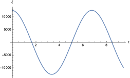
Figure 3: Time evolution of $\xi$ for $L_{4}$ in the Newtonian case.

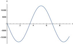
Figure 4: Time evolution of $\eta$ for $L_{4}$ in the Newtonian case.

Figure 5: Periodic orbits at linear order around the Lagrangian point $L_{4}$ in Newtonian theory.

On considering the quantum corrections evaluated in detail in Sec. II, and setting furthermore the angle $\varphi={\pi\over 4}$, while $\zeta(t=0)=2$, $\omega_{\star}=0.923$, $a_{0}=10^{-4}$, we arrive at the plots displayed in Figs. 6-8. The starting value of $\zeta$ has been taken to be $100$ km, increased gradually to reach $2500$ km.

Figure 6: Time evolution of $\xi$ for $L_{4}$ in the quantum-corrected model.

Figure 7: Time evolution of $\eta$ for $L_{4}$ in the quantum-corrected model.

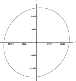
Figure 8: Periodic orbits at linear order around the Lagrangian point $L_{4}$. We have used the quantum corrected coordinates obtained at the end of Sec. II. The periodic orbit is elliptic as in the Newtonian case displayed in Fig. 5.

Our calculation is of interest because it shows that even our quantum corrected potential allows for periodic solutions in the neighborhood of uniform circular motion. The precise characterization of regions of stability and instability LeviCivita of such displaced periodic orbits is a fascinating problem for the years to come.

VI Concluding remarks and open problems

We find it appropriate to begin our concluding remarks by stressing two conceptual aspects, which are as follows. (i) In the course of an orbit of a celestial body around another celestial body, their mutual separation may change by a nonnegligible amount. Thus, it would be misleading to look for an observational test of one-loop long-distance quantum corrections to the Newtonian potential by investigating the orbits, because we do not have a formula for $V(r)$ which is equally good at all points. By contrast, the evaluation of stable equilibrium points (to first order in perturbations) provides a definite prediction, i.e., the coordinates of such a point, which can be hopefully measured with the techniques outlined in Sec. III. In other words, coordinates of Lagrangian libration points $L_{4}$ and $L_{5}$ and displaced periodic orbits around unperturbed circular motion provide a valuable test of effective field theories of quantum gravity, whereas the orbits of celestial bodies are best studied within the framework of relativistic celestial mechanics. (ii) At the risk of repeating ourselves, the technique of Refs. D94 ; D94b ; D94c ; D03 provides corrections to the Newtonian potential, and hence the unperturbed dynamics is the Newtonian celestial mechanics of the Earth-Moon-satellite system, which may provide a good example of circular restricted three-body problem. The quantum corrected potential becomes (1.2), where $k_{1}$ appears, on dimensional ground, purely classical, but includes a numerical coefficient, $\kappa_{1}$, which depends on the value taken by the coefficient $\kappa_{2}$ that multiplies $l_{P}^{2}$ in $k_{2}$:

$$\kappa_{1}=\kappa_{1}(\kappa_{2}),\;k_{2}=\kappa_{2}l_{P}^{2}.$$

Thus, we do not compute corrections to relativistic celestial mechanics (cf. Ref. Huang14 ), but, on the other hand, we need the advanced tools of relativistic celestial mechanics to test the tiny effect predicted in Eq. (2.38). We should mention at this stage the important work in Ref. Yamada12 , where the authors obtain a triangular solution to the general relativistic three-body problem for general masses, and find that the post-Newtonian configuration for three finite masses is not always equilateral. When their technique is applied to the Earth-Moon system, we find, unlike our Eq. (2.38), a correction to the $x$-coordinate of $L_{4}$ of order $2.73$ mm, and a correction to the $y$ coordinate of $L_{4}$ of order $-0.53$ mm. The former agrees with our orders of magnitude, while the latter, being less than a millimeter, is very hardly detectable.

Our original contribution is, first, the detailed calculation of the roots of the quintic equation in Sec. II (which is an original application of techniques previously developed by mathematicians), second, the derivation and solution of the nonic equation in Sec. III for quantum corrections to collinear Lagrangian points and, third, the application of the roots in Sec. II to the evaluation of displaced periodic orbits of solar sails in the Earth-Moon system, when the one-loop long distance quantum corrections to the Newtonian potentials are taken into account D03 ; BE14a ; BE14b . The use of dimensionless variables for the quintic equation (2.6), and the exploitment of exact formulas for its roots were of crucial importance to double-check the numerical predictions of Refs. BE14a ; BE14b . Interestingly, we have found that a refined analysis like ours confirms the orders of magnitude obtained in Ref. BE14b , whereas the sign of $|y_{Q}|-|y_{C}|$ gets reversed with respect to Ref. BE14b , and its expected theoretical value turns out to be smaller by $20$ per cent. Furthermore, displaced periodic orbits have been evaluated in Sec. IV with the quantum corrected coordinates displayed in Eq. (2.36), when the condition for the existence of displaced orbits is affected by terms resulting from a solar sail model. We have found that, even when the quantum corrected potential (1.2) is adopted, the displaced periodic orbits are of elliptical shape (see Fig. 8) as in the Newtonian theory. The solar-sail model is an interesting possibility considered over the last few dacades, but is not necessarily better than alternative models of planetoid. For example, the large structure and optical nature of solar sails can create a considerable challenge. If the structure and mass distribution of the sail is complicated, one has to resort to suitable approximations. Furthermore, the characterization of regions of stability or instability LeviCivita of displaced periodic orbits of solar sails is a theoretical problem whose solution might have far reaching consequences for designing space missions.

Last, but not least, the laser ranging techniques outlined in Sec. IV appear as a promising tool for testing the predictions at the end of Sec. II. The years to come will hopefully tell us whether a laser ranging test mass can be designed, upon consideration of the four key performance indicators listed at the end of Sec. IV. At that stage, the task will remain to actually send a satellite at $L_{4}$ and keep it there despite the perturbations caused by the Sun Tapley , which has never been accomplished to the best of our knowledge. The resulting low-energy test of quantum gravity in the solar system would reward the considerable effort necessary to achieve this.

Appendix A Bring-Jerrard form of quintic equations

Let us start from the general quintic equation

$$X^{5}+a_{4}X^{4}+a_{3}X^{3}+a_{2}X^{2}+a_{1}X+a_{0}=0.$$ (115)

Denote the roots of Eq. (A1) by $X_{i},i=1,...,5$, and let

$$S_{n}=S_{n}(X_{k})\equiv\sum_{k=1}^{5}(X_{k})^{n}$$ (116)

be the sum of the $n$th powers of such roots. By virtue of the Newton power-sum formula, a general representation of $S_{n}$ is

$$S_{n}=-na_{5-n}-\sum_{j=1}^{n-1}S_{n-j}a_{5-j},$$ (117)

with the understanding that $a_{j}=0$ for $j<0$. For the lowest values of $n$, Eq. (A3) yields $S_{1}(X_{k})=-a_{4},\;S_{2}(X_{k})=(a_{4})^{2}-2a_{3},\;S_{3}(X_{k})=-(a_{4})^{3}+3a_{3}a_{4}-3a_{2}$,

$$S_{4}(X_{k})=(a_{4})^{4}-4a_{3}(a_{4})^{2}+4a_{2}a_{4}+2(a_{3})^{2}-4a_{1},$$ (118)

$$S_{5}(X_{k})=-(a_{4})^{5}+5\Bigr{[}a_{3}(a_{4})^{3}-a_{2}(a_{4})^{2}-(a_{3})^{2}a_{4}+a_{1}a_{4}-a_{0}+a_{2}a_{3}\Bigr{]}.$$ (119)

A systematic way to proceed involves two steps, i.e., first a quadratic Tschirnhaus transformation T

$$Y_{k}=(X_{k})^{2}+\mu X_{k}+\nu$$ (120)

between the roots $X_{k}$ of Eq. (A1) and the roots $Y_{k}$ of the principal quintic

$$X^{5}+c_{2}X^{2}+c_{1}X+c_{0}=0,$$ (121)

supplemented Adamchik by the evaluation of $S_{1}(Y_{k}),...,S_{5}(Y_{k})$ to obtain through radicals $\mu,\nu,c_{0},c_{1},c_{2}$, and eventually a quartic Tschirnhaus transformation T

$$Z_{k}=(Y_{k})^{4}+u_{1}(Y_{k})^{3}+u_{2}(Y_{k})^{2}+u_{3}Y_{k}+u_{4},$$ (122)

between the roots $Y_{k}$ of Eq. (A7) and the roots $Z_{k}$ of the Bring-Jerrard form (2.10) of the quintic. This procedure is conceptually clear although rather lengthy (see Appendix B), and the joint effect of inverting (A8) and then (A6) to find $X_{k}=X_{k}(Y_{j}(Z_{l}))$ leads to $20$ candidate roots Adamchik , which is not very helpful if one is interested in the numerical values of such roots, as indeed we are. One might instead stick to our Eq. (2.6) and then try to exploit the Birkeland theorem Birkeland1920 , according to which the roots of any quintic can be re-expressed through generalized hypergeometric functions like the ones defined in our Sec. II. However, when there are three (or more) nonvanishing coefficients as in Eq. (2.6), the Birkeland theorem leads to too many (for numerical purposes) hypergeometric functions in the general expansion of roots. Furthermore, the set of linear partial differential equations Sturmfels obeyed by the roots when viewed as functions of all coefficients does not lead easily to their explicit form.

At this stage, having appreciated the need for a trinomial, possibly Bring-Jerrard form of the quintic, and rather than feeling in despair, we point out that, since in our original quintic (2.6) two coefficients vanish, i.e. $a_{2}=a_{1}=0$, it is more convenient to use what is normally ruled out in the generic case Adamchik , i.e., a cubic Tschirnhaus transformation between the roots $X_{k}$ of Eq. (A1) and the roots $Y_{k}$ of Eq. (2.10):

$$Y_{k}=(X_{k})^{3}+\lambda_{1}(X_{k})^{2}+\lambda_{2}(X_{k})+\lambda_{3}.$$ (123)

By virtue of Eqs. (2.10) and (A2)-(A5), we find

$$S_{1}(Y_{k})=S_{2}(Y_{k})=S_{3}(Y_{k})=0,$$ (124)

$$S_{4}(Y_{k})=-4d_{1},\;S_{5}(Y_{k})=-5d_{0}.$$ (125)

On assuming the cubic relation (A9), Eqs. (A10) become a nonlinear algebraic system leading to the numerical evaluation of $\lambda_{1},\lambda_{2},\lambda_{3}$. More precisely, from $S_{1}(Y_{k})=0$ we find

$$5\lambda_{3}+\lambda_{2}S_{1}(X_{k})+\lambda_{1}S_{2}(X_{k})+S_{3}(X_{k})=0,$$ (126)

while from $S_{2}(Y_{k})=0$ we obtain

$$5(\lambda_{3})^{2}+2\lambda_{2}\lambda_{3}S_{1}(X_{k})+[(\lambda_{2})^{2}+2\lambda_{1}\lambda_{3}]S_{2}(X_{k})+2(\lambda_{1}\lambda_{2}+\lambda_{3})S_{3}(X_{k})$$ (127)

$$+ [(\lambda_{1})^{2}+2\lambda_{2}]S_{4}(X_{k})+2\lambda_{1}S_{5}(X_{k})+S_{6}(X_{k})=0.$$

Last, from the vanishing of $S_{3}(Y_{k})$ we get

$$5(\lambda_{3})^{3}+3\lambda_{2}(\lambda_{3})^{2}S_{1}(X_{k})+3(\lambda_{2})^{2}\lambda_{3}S_{2}(X_{k})+(\lambda_{2})^{3}S_{3}(X_{k})$$ (128)

$$+ 3(\lambda_{1})^{2}\lambda_{3}S_{4}(X_{k})+[3(\lambda_{1})^{2}\lambda_{2}+6\lambda_{1}\lambda_{3}]S_{5}(X_{k})+[(\lambda_{1})^{3}+3\lambda_{3}+6\lambda_{1}\lambda_{2}]S_{6}(X_{k})$$

$$+ 3[(\lambda_{1})^{2}+\lambda_{2}]S_{7}(X_{k})+3\lambda_{1}S_{8}(X_{k})+S_{9}(X_{k})=0.$$

The system (A12)-(A14) cannot be solved by radicals because, if one expresses for example $\lambda_{1}$ as a linear function of $\lambda_{2}$ and $\lambda_{3}$ from Eq. (A12), and one solves the resulting quadratic equation for $\lambda_{2}=\lambda_{2}(\lambda_{3})$ or $\lambda_{3}=\lambda_{3}(\lambda_{2})$ from Eq. (A13), one discovers that Eq. (A14) is not a polynomial in $\lambda_{3}$ (respectively, $\lambda_{2}$). Nevertheless, for numerical purposes, the system (A12)-(A14) can be solved and has been solved from us in the Earth-Moon system. Last, from Eq. (A11) we find the coefficients $d_{1}$ and $d_{0}$ in the Bring-Jerrard form of the quintic, according to the formulas

$$d_{1}=-{1\over 4}S_{4}(Y_{k})=\sum_{i=0}^{12}b_{1i}S_{i}(X_{k}),$$ (129)

$$d_{0}=-{1\over 5}S_{5}(Y_{k})=\sum_{i=0}^{15}b_{0i}S_{i}(X_{k}),$$ (130)

We have evaluated all $b_{1i}$ and $b_{0i}$ coefficients by applying patiently the Tschirnhaus transformation (A9) and the definition (A2). We find therefore six triplets of possible values for $\lambda_{1},\lambda_{2},\lambda_{3}$ (see Tables I and II), which lead always to the same values of $d_{1}$ and $d_{0}$ (this is a crucial consistency check), i.e.

$$d_{1}(w)=2.78\cdot 10^{-176}+{\rm i}6.91\cdot 10^{-186},\;d_{1}(u)=2.78\cdot 10^{-176}-{\rm i}8.51\cdot 10^{-188},$$ (131)

$$d_{0}(w)=1.66\cdot 10^{-220}-{\rm i}5.17\cdot 10^{-230},\;d_{0}(u)=-1.66\cdot 10^{-220}+{\rm i}6.36\cdot 10^{-232},$$ (132)

where $w$ and $u$ are the variables defined in Eqs. (2.5) and (2.32), respectively. Eventually, the roots $X_{k}$ of our quintic (2.6) have been obtained by solving Eq. (A9) for $X_{k}=X_{k}(Y_{k})$, with the help of the solution algorithm for the cubic equation. This means that we first re-express (A9) in the form

$$h(X_{k})\equiv(X_{k})^{3}+\kappa_{2}(X_{k})^{2}+\kappa_{1}X_{k}+\kappa_{0}=0,$$ (133)

where $\kappa_{2}\equiv\lambda_{1},\kappa_{1}\equiv\lambda_{2},\kappa_{0}\equiv\lambda_{3}-Y_{k}$. We then define the new variable

$$V_{k}\equiv X_{k}+{\kappa_{2}\over 3}=X_{k}+{\lambda_{1}\over 3},$$ (134)

in terms of which Eq. (A19) is mapped into its canonical form

$$(V_{k})^{3}+pV_{k}+q=0,\;p\equiv h^{\prime}\left(-{\kappa_{2}\over 3}\right),\;q\equiv h\left(-{\kappa_{2}\over 3}\right).$$ (135)

As shown in Ref. Birkeland1924 , if the discriminant

$$\delta\equiv-{27\over 4}{q^{2}\over p^{3}}$$ (136)

is such that $|\delta|<1$, or if $\delta=1$, the three roots of Eq. (A21) can be expressed through the Gauss hypergeometric function in the form

$$(V_{k})_{i}=\sqrt{-p}\left[(-1)^{3i}F\left(-{1\over 6},{1\over 6},{1\over 2};\delta\right)+{1\over 3}\sqrt{\delta\over 3}F\left({1\over 3},{2\over 3},{3\over 2};\delta\right)\right](i=1,2),$$ (137)

$$(V_{k})_{3}=-{2\over 3}\sqrt{-{p\delta\over 3}}\;F\left({1\over 3},{2\over 3},{3\over 2};\delta\right).$$ (138)

As is clear from (A20), (A23), (A24), our method yields eventually $15$ candidate roots, and by insertion into the original quintic (2.6) we have found the $5$ effective roots at the end of Sec. II.

Table 1: The six triplets of values of $\lambda_{3}$, $\lambda_{2}$ and $\lambda_{1}$ for the $1/r$-equation (2.1).

$n$th triplet	$\lambda_{3}$	$\lambda_{2}$	$\lambda_{1}$
n=1	$-4.98\times 10^{45}-3.10\times 10^{-55}\;\mathrm{i}$	$0.26+1.59\times 10^{-11}\;\mathrm{i}$	$4.21\times 10^{32}+3.78\times 10^{-44}\;\mathrm{i}$
n=2	$-4.98\times 10^{-45}+3.10\times 10^{-55}\;\mathrm{i}$	$0.26-1.59\times 10^{-11}\;\mathrm{i}$	$4.21\times 10^{32}-3.78\times 10^{-44}\;\mathrm{i}$
n=3	$2.49\times 10^{-45}+4.32\times 10^{-45}\;\mathrm{i}$	$0.26+2.57\times 10^{-11}\;\mathrm{i}$	$4.21\times 10^{32}+6.11\times 10^{-44}\;\mathrm{i}$
n=4	$2.49\times 10^{-45}-4.32\times 10^{-45}\;\mathrm{i}$	$0.26-2.57\times 10^{-11}\;\mathrm{i}$	$4.21\times 10^{32}-6.11\times 10^{-44}\;\mathrm{i}$
n=5	$2.49\times 10^{-45}+4.32\times 10^{-45}\;\mathrm{i}$	$0.26+9.82\times 10^{-12}\;\mathrm{i}$	$4.21\times 10^{32}+2.34\times 10^{-44}\;\mathrm{i}$
n=6	$2.49\times 10^{-45}-4.32\times 10^{-45}\;\mathrm{i}$	$0.26-9.82\times 10^{-12}\;\mathrm{i}$	$4.21\times 10^{32}-2.34\times 10^{-44}\;\mathrm{i}$

Table 2: The six triplets of values of $\lambda_{3}$, $\lambda_{2}$ and $\lambda_{1}$ for the $1/s$-equation (2.2).

$n$th triplet	$\lambda_{3}$	$\lambda_{2}$	$\lambda_{1}$
n=1	$-4.98\times 10^{-45}-3.82\times 10^{-57}\;\mathrm{i}$	$0.26+1.96\times 10^{-13}\;\mathrm{i}$	$5.17\times 10^{30}+3.78\times 10^{-44}\;\mathrm{i}$
n=2	$-4.98\times 10^{-45}+3.82\times 10^{-57}\;\mathrm{i}$	$0.26-1.96\times 10{-13}\;\mathrm{i}$	$5.17\times 10^{30}-3.78\times 10^{-44}\;\mathrm{i}$
n=3	$2.49\times 10^{-45}+4.32\times 10^{-45}\;\mathrm{i}$	$0.26+3.16\times 10^{-13}\;\mathrm{i}$	$5.17\times 10^{30}+6.11\times 10^{-44}\;\mathrm{i}$
n=4	$2.49\times 10^{-45}-4.32\times 10^{-45}\;\mathrm{i}$	$0.26-3.16\times 10^{-13}\;\mathrm{i}$	$5.17\times 10^{30}-6.11\times 10^{-44}\;\mathrm{i}$
n=5	$2.49\times 10^{-45}+4.32\times 10^{-45}\;\mathrm{i}$	$0.26+1.21\times 10^{-13}\;\mathrm{i}$	$5.17\times 10^{30}+2.34\times 10^{-44}\;\mathrm{i}$
n=6	$2.49\times 10^{-45}-4.32\times 10^{-45}\;\mathrm{i}$	$0.26-1.21\times 10^{-13}\;\mathrm{i}$	$5.17\times 10^{30}-2.34\times 10^{-44}\;\mathrm{i}$

Yet another valuable solution algorithm is available, i.e. the method in Ref. King which expresses the roots of the quintic (A1) through two infinite series, i.e., the Jacobi nome and the theta series, for which fast convergence is obtained, but the need to evaluate the roots with a large number of decimal digits makes it problematic, as far as we can see, to deal with such series. Further valuable work on the quintic can be found in Ref. Drociuk .

Appendix B Alternative route to the quintic

We here find it useful to give details about the main alternative to the procedure used in Appendix A. For that purpose, as we said, one assumes that the roots $X_{k}$ of Eq. (A1) are related to the roots $Y_{k}$ of the principal quintic (A7) by the quadratic transformation (A6). The power sums for the principal quintic form are indeed

$$S_{1}(Y_{k})=S_{2}(Y_{k})=0,\;S_{3}(Y_{k})=-3c_{2},\;S_{4}(Y_{k})=-4c_{1},\;S_{5}(Y_{k})=-5c_{0}.$$ (139)

On the other hand, we can evaluate $S_{1}(Y_{k})$ and $S_{2}(Y_{k})$ by using the quadratic transformation (A6) and exploiting the identities

$$S_{1}(Y_{k})=S_{2}(X_{k})+\mu S_{1}(X_{k})+5\nu,$$ (140)

$$S_{2}(Y_{k})=S_{4}(X_{k})+2\mu S_{3}(X_{k})+(\mu^{2}+2\nu)S_{2}(X_{k})+2\mu\nu S_{1}(X_{k})+5\nu^{2},$$ (141)

obtaining therefore the following equations for $\mu$ and $\nu$:

$$\mu a_{4}-5\nu+2a_{3}-(a_{4})^{2}=0,$$ (142)

$$\mu^{2}a_{3}-10\nu^{2}+\mu(3a_{2}-a_{3}a_{4})+2a_{1}-2a_{2}a_{4}+(a_{3})^{2}=0,$$ (143)

where, in the course of arriving at Eq. (B5), we have re-expressed repeatedly $(a_{4})^{2}$ from Eq. (B4). This system is quadratic with respect to $\mu$ and $\nu$, and hence leads to two sets of coefficients. For the case studied in Eq. (2.6), they reduce to (here $a_{3}=\rho_{3},a_{4}=\rho_{4}$)

$$\mu_{\pm}={a_{4}[13a_{3}-4(a_{4})^{2}]\pm\sqrt{60(a_{3})^{3}-15(a_{3}a_{4})^{2}}\over 2[5a_{3}-2(a_{4})^{2}]},$$ (144)

$$\nu_{\pm}={\mu_{\pm}\over 5}a_{4}+{2\over 5}a_{3}-{1\over 5}(a_{4})^{2}.$$ (145)

There is complete freedom to choose either of these. After finding $\mu$ and $\nu$ in such a way, one can use the Eqs. (B1) to obtain $c_{0},c_{1},c_{2}$. One finds explicitly, in general,

$$c_{0} = -\nu^{5}-\mu\nu^{4}S_{1}(X_{k})-(2\mu^{2}\nu^{3}+\nu^{4})S_{2}(X_{k})-\left(2\mu^{3}\nu^{2}+4\mu\nu^{3}\right)S_{3}(X_{k})$$ (146)

$$- \left(\mu^{4}\nu+6\mu^{2}\nu^{2}+2\nu^{3}\right)S_{4}(X_{k})-\left({\mu^{5}\over 5}+4\mu^{3}\nu+6\mu\nu^{2}\right)S_{5}(X_{k})$$

$$- (\mu^{4}+6\mu^{2}\nu+2\nu^{2})S_{6}(X_{k})-(2\mu^{3}+4\mu\nu)S_{7}(X_{k})-(2\mu^{2}+\nu)S_{8}(X_{k})$$

$$- \mu S_{9}(X_{k})-{1\over 5}S_{10}(X_{k}),$$

$$c_{1} = -{5\over 4}\nu^{4}-\mu\nu^{3}S_{1}(X_{k})-\left({3\over 2}\mu^{2}\nu^{2}+\nu^{3}\right)S_{2}(X_{k})$$ (147)

$$- (\mu^{3}\nu+3\mu\nu^{2})S_{3}(X_{k})-\left({\mu^{2}\over 4}+3\mu^{2}\nu+{3\over 2}\nu^{2}\right)S_{4}(X_{k})-(\mu^{3}+3\mu\nu)S_{5}(X_{k})$$

$$- \left({3\over 2}\mu^{2}+\nu\right)S_{6}(X_{k})-\mu S_{7}(X_{k})-{1\over 4}S_{8}(X_{k}),$$

$$c_{2} = -{5\over 3}\nu^{3}-\mu\nu^{2}S_{1}(X_{k})-(\mu^{2}\nu+\nu^{2})S_{2}(X_{k})-{\mu\over 3}(\mu^{2}+6\nu)S_{3}(X_{k})$$ (148)

$$- (\mu^{2}+\nu)S_{4}(X_{k})-\mu S_{5}(X_{k})-{1\over 3}S_{6}(X_{k}).$$

The removal from a general quintic of the three terms in $X^{4},X^{3}$ and $X^{2}$ brings it to the Bring-Jerrard form (2.10), here re-written for convenience as

$$X^{5}+d_{1}X+d_{0}=0.$$ (149)

By virtue of the Newton formulas (A3), the power sums for the quintic (B11) are

$$S_{1}(Z_{k})=S_{2}(Z_{k})=S_{3}(Z_{k})=0,\;S_{4}(Z_{k})=-4d_{1},\;S_{5}(Z_{k})=-5d_{0}.$$ (150)

Assuming now, following Bring Bring , that the roots $Z_{k}$ of Eq. (B11) are related by the quartic transformation (A8) to the roots $Y_{k}$ of the principal quintic (A7), we can substitute Eq. (A8) into Eq. (B12). This leads to a system of five equations with six unknown variables. More precisely, from the equation

$$S_{1}(Z_{k})=5u_{4}-4c_{1}-3u_{1}c_{2}=0,$$ (151)

one finds

$$u_{4}={4\over 5}c_{1}+{3\over 5}c_{2}u_{1}.$$ (152)

The second equation Adamchik

$$S_{2}(Z_{k}) = -10u_{1}u_{2}c_{0}-4(u_{2})^{2}c_{1}+{4\over 5}(c_{1})^{2}+8c_{0}c_{2}+{46\over 5}u_{1}c_{1}c_{2}$$ (153)

$$+ \left[{6\over 5}(u_{1})^{2}+6u_{2}\right](c_{2})^{2}-2u_{3}(5c_{0}+4u_{1}c_{1}+3u_{2}c_{2})=0,$$

obtained from the identities

$$S_{2}(Z_{k}) = S_{8}(Y_{k})+2u_{1}S_{7}(Y_{k})+[(u_{1})^{2}+2u_{2}]S_{6}(Y_{k})+2(u_{1}u_{2}+u_{3})S_{5}(Y_{k})$$ (154)

$$+ [(u_{2})^{2}+2u_{4}+2u_{1}u_{3}]S_{4}(Y_{k})+2(u_{2}u_{3}+u_{1}u_{4})S_{3}(Y_{k})+5(u_{4})^{2},$$

$$S_{6}(Y_{k})=3(c_{2})^{2},\;S_{7}(Y_{k})=7c_{1}c_{2},\;S_{8}(Y_{k})=8c_{0}c_{2}+4(c_{1})^{2},$$ (155)

relates $u_{2}$ and $u_{3}$. The clever idea of the Bring-Jerrard method lies in choosing $u_{2}$ in such a way that the coefficient of $u_{3}$ in Eq. (B15) vanishes. By inspection one finds immediately

$$u_{2}=-{5\over 3}{c_{0}\over c_{2}}-{4\over 3}{c_{1}\over c_{2}}u_{1}.$$ (156)

Thus, Eq. (B15) now depends only on $u_{1}$ and is a quadratic, i.e. Adamchik

$$\Bigr{[}27(c_{2})^{4}-160(c_{1})^{3}+300c_{0}c_{1}c_{2}\Bigr{]}(u_{1})^{2}+\Bigr{[}27c_{1}(c_{2})^{3}-400c_{0}(c_{1})^{2}+375(c_{0})^{2}c_{2}\Bigr{]}u_{1}$$ (157)

$$+ 18(c_{1}c_{2})^{2}-45c_{0}(c_{2})^{3}-250(c_{0})^{2}c_{1}=0.$$

Last, by setting the sum of the cubes of (A8) to zero by virtue of (B12), a cubic equation for $u_{3}$ is obtained, by virtue of the identity

$$S_{3}(Z_{k})=5(u_{4})^{3}+\sum_{l=2}^{12}b_{l}S_{l}(Y_{k}),$$ (158)

where (recall that we already know $S_{1}(Y_{k})...S_{8}(Y_{k})$)

$$b_{2}=3u_{2}(u_{4})^{2},$$ (159)

$$b_{3}=(u_{3})^{3}+3u_{1}(u_{4})^{2}+6u_{2}u_{3}u_{4},$$ (160)

$$b_{4}=3(u_{2})^{2}u_{4}+3(u_{4})^{2}+3u_{2}(u_{3})^{2}+6u_{1}u_{3}u_{4},$$ (161)

$$b_{5}=3(u_{2})^{2}u_{3}+3u_{1}(u_{3})^{2}+6u_{4}(u_{3}+u_{1}u_{2}),$$ (162)

$$b_{6}=(u_{2})^{3}+3(u_{1})^{2}u_{4}+3(u_{3})^{2}+6u_{2}(u_{4}+u_{1}u_{3}),$$ (163)

$$b_{7}=3(u_{1})^{2}u_{3}+3(u_{2})^{2}u_{1}+6(u_{1}u_{4}+u_{2}u_{3}),$$ (164)

$$b_{8}=3u_{4}+3(u_{1})^{2}u_{2}+3(u_{2})^{2}+6u_{1}u_{3},$$ (165)

$$b_{9}=(u_{1})^{3}+3u_{3}+6u_{1}u_{2},$$ (166)

$$b_{10}=3u_{2}+3(u_{1})^{2},$$ (167)

$$b_{11}=3u_{1},$$ (168)

$$b_{12}=1,$$ (169)

$$S_{9}(Y_{k})=9c_{0}c_{1}-3(c_{2})^{3},$$ (170)

$$S_{10}(Y_{k})=5(c_{0})^{2}-10c_{1}(c_{2})^{2},$$ (171)

$$S_{11}(Y_{k})=-11c_{0}(c_{2})^{2}-11(c_{1})^{2}c_{2},$$ (172)

$$S_{12}(Y_{k})=-24c_{0}c_{1}c_{2}-4(c_{1})^{3}+3(c_{2})^{4}.$$ (173)

All intermediate quantities for reduction to the Bring-Jerrard form can be therefore found in terms of radicals. Of course, once the irreducible quintic (B11) is solved in terms of hypergeometric functions as outlined in Sec. II, one has to invert the Tschirnaus-Bring quartic transformation (A8) to obtain the solutions of the principal quintic (A7) and, eventually, of the original quintic (A1), i.e.,

$$X_{k}=X_{k}(Y_{j}(Z_{l})).$$ (174)

Thus, one obtains in general twenty candidates for five solutions, and only numerical testing can tell which ones are correct Adamchik .

References

- (1) A. Einstein, Annalen Phys. 49, 769 (1916).
- (2) Y. Choquet-Bruhat, General Relativity and the Einstein Equations (Oxford University Press, Oxford, 2009).
- (3) A. S. Wightman, Fortschr. Phys. 44, 173 (1996).
- (4) J. Polchinski, String Theory (Cambridge University Press, Cambridge, 1998).
- (5) C. Rovelli, Quantum Gravity (Cambridge University Press, Cambridge, 2004).
- (6) R. Penrose and M. A. H. MacCallum, Phys. Rep. 6 C, 241 (1973).
- (7) G. Esposito, An Introduction to Quantum Gravity, UNESCO Encyclopedia (UNESCO, Paris, France, 2011).
- (8) B. S. DeWitt, Phys. Rev. 162, 1239 (1967).
- (9) C. Kiefer and M. Kramer, Phys. Rev. Lett. 108, 021301 (2012).
- (10) D. Bini, G. Esposito, K. Kiefer, M. Kramer, and F. Pessina, Phys. Rev. D 87, 104008 (2013).
- (11) D. Bini and G. Esposito, Phys. Rev. D 89, 084032 (2014).
- (12) A. Yu. Kamenshchik, A. Tronconi, and G. Venturi, Phys. Lett. B 726, 518 (2013).
- (13) A. Yu. Kamenshchik, A. Tronconi, and G. Venturi, Phys. Lett. B 734, 72 (2014).
- (14) A. Ashoorioon, P. S. Bhupal Dev, and A. Mazumdar, Mod. Phys. Lett. A 29, 1450163 (2014); L. Krauss and F. Wilczek, Phys. Rev. D 89, 047501 (2014).
- (15) J. F. Donoghue, Phys. Rev. Lett. 72, 2996 (1994).
- (16) J. F. Donoghue, Phys. Rev. D 50, 3874 (1994).
- (17) J. F. Donoghue, arXiv:gr-qc/9405057.
- (18) I. J. Muzinich and S. Vokos, Phys. Rev. D 52, 3472 (1995).
- (19) H. W. Hamber and S. Liu, Phys. Lett. B 357, 51 (1995).
- (20) A. A. Akhundov, S. Bellucci, and A. Shiekh, Phys. Lett. B 395, 16 (1997).
- (21) I. B. Khriplovich and G. G. Kirilin, Sov. Phys. JETP 95, 981 (2002).
- (22) N. E. J. Bjerrum-Bohr, J. F. Donoghue, and B. R. Holstein, Phys. Rev. D 67, 084033 (2003).
- (23) E. Battista and G. Esposito, Phys. Rev. D 89, 084030 (2014).
- (24) E. Battista and G. Esposito, Phys. Rev. D 90, 084010 (2014).
- (25) H. Poincaré, Acta Mathematica 13, 1 (1890); Bull. Astronomique 8, 12 (1891).
- (26) H. Poincaré, Les Methodes Nouvelles de la Mecanique Celeste (Gauthier-Villars, Paris, 1892), reprinted as New Methods of Celestial Mechanics, edited by D. L. Goroff (American Institute of Physics, College Park, 1993).
- (27) L. A. Pars, A Treatise on Analytical Dynamics (Heinemann, London, 1965).
- (28) E. V. Pitjeva, in Relativity in Fundamental Astronomy, Proceedings IAU Symposium No. 261, Eds. S. A Klioner, P. K. Seidelman, and M. H. Soffel, 2009.
- (29) J. Simo and C. R. McInnes, in 59th International Astronomical Congress, Glasgow, Scotland, 2008.
- (30) J. Simo and C. R. McInnes, Comm. Nonlinear Sci. Numer. Simulat. 14, 4191 (2009).
- (31) J. Simo and C. R. McInnes, J. of Guidance, Control, and Dynamics 32, 1666 (2009).
- (32) J. Simo and C. R. McInnes, J. of Guidance, Control, and Dynamics 33, 259 (2010).
- (33) J. Simo and C. R. McInnes, Acta Astronautica 96, 106 (2014).
- (34) C. R. McInnes, Solar Sailing: Technology, Dynamics and Mission Applications (Springer Praxis, London, 1999).
- (35) T. Waters and C. R. McInnes, J. of Guidance, Control, and Dynamics 30, 687 (2007).
- (36) V. Szebehely, Theory of Orbits: the Restricted Problem of Three Bodies (Academic Press, New York, 1967).
- (37) A. E. Roy, Orbital Motion (Institute of Physics Publishing, Philadelphia, 2005).
- (38) F. O. Vonbun, NASA report TN-D-4468 (1968).
- (39) R. Thurman and P. Worfolk, Technical report GC95, Geometry Center, University of Minnesota (1996).
- (40) G. Gomez, J. Libre, R. Martinez, and C. Simo, Dynamics and Mission Design Near Libration Points, Vol. I, II (World Scientific, Singapore, 2001).
- (41) G. Gomez, A. Jorba, J. Masdemont, and C. Simo, Dynamics and Mission Design Near Libration Points, Vol. III, IV (World Scientific, Singapore, 2001).
- (42) R. W. Farquhar and A. A. Kamel, Cel. Mech. 7, 458 (1973).
- (43) R. W. Farquhar, NASA technical report (1971).
- (44) J. V. Breakwell and J. V. Brown, Cel. Mech. 20, 389 (1979).
- (45) D. L. Richardson, J. Guidance and Control 3, 543 (1980).
- (46) K. C. Howell, Cel. Mech. 32, 53 (1984).
- (47) K. C. Howell and B. G. Marchand, Dyn. Systems: An Int. J. 20, 149 (2005).
- (48) C. McInnes, J. of Spacecraft and Rocket 30, 782 (1993).
- (49) E. S. Bring, Quart. J. Math. 6 (1864).
- (50) G. B. Jerrard, An Essay on the Resolution of Equations (Taylor and Francis, New York, 1859).
- (51) C. Hermite, Comptes Rendus Acad. Sci. Paris 46, 508 (1858).
- (52) R. Birkeland, in International Congress of Mathematicians (1924).
- (53) B. D. Tapley and J. M. Lewallen, AIAA J. 2, 728 (1964).
- (54) Z. Altamimi, X. Collilieux, J. Legrand et al., J. Geophys. Res. 112, B09401 (2007).
- (55) M. R. Pearlman, J. J. Degnan, and J. M. Bosworth, Adv. Space Res. 30, 135 (2002).
- (56) P. L. Bender et al., Science 182, 229 (1973).
- (57) J. G. Williams, S. G. Turyshev, and D. H. Boggs, Phys. Rev. Lett. 93, 261101 (2004).
- (58) I. I. Shapiro, R. D. Reasenberg, J. F. Chandler, and R. W. Babcock, Phys. Rev. Lett. 61, 2643 (1988).
- (59) S. Dell’Agnello et al., Nucl. Instr. Methods Phys. Res. A 692, 275 (2012).
- (60) M. Martini, S. Dell’Agnello et al., Planet Space Sci. 74, 276 (2012).
- (61) R. March, G. Bellettini, R. Tauraso, and S. Dell’Agnello, Phys. Rev. D 83, 104008 (2011).
- (62) R. March, G. Bellettini, R. Tauraso, and S. Dell’Agnello, Gen. Relativ. Gravit. 43, 3099 (2011).
- (63) S. Dell’Agnello et al., J. Adv. Space Res. 47, 822 (2011).
- (64) S. Dell’Agnello et al., in ESA Proc. Int. Conf. on Space Optics (Tenerife, Spain, Oct. 2014).
- (65) D. Currie, S. Dell’Agnello, G. O. Delle Monache, B. Behr, and J. G. Williams, Nucl. Phys. B Proc. Suppl. 243, 218 (2013).
- (66) S. Dell’Agnello et al., Exp. Astron. 32, 19 (2011).
- (67) D. Vokrouhlicky, Icarus 126, 293 (1997).
- (68) G. Huang and X. Wu, Phys. Rev. D 89, 124034 (2014).
- (69) K. Yamada and H. Asada, Phys. Rev. D 86, 124029 (2012).
- (70) T. Levi Civita, Opere Matematiche, Vol. II (Zanichelli, Bologna, 1956).
- (71) E. Tschirnhaus, ACM SIGSAM Bulletin 37, N. 143, 1 (2003).
- (72) V. S. Adamchik and D. J. Jeffrey, ACM SIGSAM Bulletin 37, N. 3, 90 (2003).
- (73) R. Birkeland, Comptes Rendus Acad. Sciences Paris 171, 1370 (1920).
- (74) B. Sturmfels, Discrete Math. 210, 171 (2000).
- (75) R. B. King and E. R. Canfield, J. Math. Phys. 32, 823 (1991).
- (76) R. Drociuk, arXiv:math/0207058 [math.GM].