Emergence of electromotive force in precession-less rigid motion of deformed domain wall

Abstract

Recently it has been recognized that the electromotive force (emf) can be induced just by the spin precession where the generation of the electromotive force has been considered as a real-space topological pumping effect. It has been shown that the amount of the electromotive force is independent of the functionality of the localized moments. It was also demonstrated that the rigid domain wall (DW) motion cannot generate electromotive force in the system. Based on real-space topological pumping approach in the current study we show that the electromotive force can be induced by rigid motion of a deformed DW. We also demonstrate that the generated electromotive force strongly depends on the DW bulging. Meanwhile results show that the DW bulging leads to generation of the electromotive force both along the axis of the DW motion and normal to the direction of motion.

1 Introduction

One of the powerful techniques in condensed matter physics is based on the manifestation of Berry phase in electronic systems berry1984quantal ; xiao2010berry ; wilczek1989geometric ; bohm2003geometric . Berry curvature in momentum space $\Omega_{kk}$ give rise to the anomalous Hall effect nagaosa2010anomalous , in which the Berry phase concept behave as a link between anomalous Hall effect and topological nature of the Hall currents. This effect quantitatively has been calculated by $abinitio$ methods in Refs. turek2012ab ; weischenberg2011ab ; lowitzer2010coherent ; wang2006ab ; yao2004first . As reported in Ref. neubauer2009topological topological Hall effect is described by real space Berry curvature in which emergent real space Berry curvature acts like a real magnetic field. This effect has also been observed experimentally in several studies of this field kanazawa2011large ; neubauer2009topological ; muhlbauer2009skyrmion ; huang2012extended .

In phase space, an adiabatic evolution of a wave packet generates various interesting Berry phase effects sundaram1999wave . The evolution of the wave packet center $(r_{c},k_{c})$ in phase space is describe by a set of semi-classical equations,

$$\frac{\partial{\boldsymbol{{r}}_{c}}}{\partial t}=\frac{\partial E({\boldsymbol{{r}}_{c}},{\boldsymbol{{k}}_{c}})}{\hbar\partial{\boldsymbol{{k}}_{c}}}-\left(\overset{\scriptscriptstyle\leftrightarrow}{\boldsymbol{\Omega}}_{\boldsymbol{kr}}\cdot\frac{\partial{\boldsymbol{{r}}_{c}}}{\partial t}+\overset{\scriptscriptstyle\leftrightarrow}{\boldsymbol{\Omega}}_{\boldsymbol{kk}}\cdot\frac{\partial{\boldsymbol{{k}}_{c}}}{\partial t}\right)-{{\boldsymbol{\Omega}}_{\boldsymbol{k}t}}$$ (1)

$$\frac{\partial{\boldsymbol{{k}}_{c}}}{\partial t}=-\frac{\partial E({\boldsymbol{{r}}_{c}},{\boldsymbol{{k}}_{c}})}{\hbar\partial{\boldsymbol{{r}}_{c}}}+\left(\overset{\scriptscriptstyle\leftrightarrow}{\boldsymbol{\Omega}}_{\boldsymbol{rr}}\cdot\frac{\partial{\boldsymbol{{r}}_{c}}}{\partial t}+\overset{\scriptscriptstyle\leftrightarrow}{\boldsymbol{\Omega}}_{\boldsymbol{rk}}\cdot\frac{\partial{\boldsymbol{{k}}_{c}}}{\partial t}\right)-{{\boldsymbol{\Omega}}_{\boldsymbol{r}t}},$$ (2)

where the energy of the wave packet is $E({\boldsymbol{{r}}_{c}},\boldsymbol{k}_{c})$ and $\overset{\scriptscriptstyle\leftrightarrow}{\boldsymbol{\Omega}}$ is the Berry curvature tensor. The Berry curvature tensor in terms of for $(r,t)$ is defined by

$$\Omega_{rt}=\frac{\partial}{\partial r}A_{t}-\frac{\partial}{\partial t}A_{r}$$ (3)

where

$$A_{t}=i\left\langle u_{k}\right|\frac{\partial}{\partial t}\left|u_{k}\right\rangle$$ (4)

and

$$A_{r}=i\left\langle u_{k}\right|\frac{\partial}{\partial r}\left|u_{k}\right\rangle$$ (5)

known as Berry connections (gauge potentials), $\left|u_{k}\right\rangle$ is periodic part of the Bloch eigenstate of selected band. We have focused on space-time Berry curvature, $\Omega_{rt}$, which determines the emf of the sample. The emf in terms of Berry curvature is described in Refs. stern1992berry ; barnes2007generalization ; MacDonald where the emf along a path $l$ can be calculated by

$$emf={-\hbar}/{e}\int_{l}{dr\cdot{{\Omega}_{rt}}}.$$ (6)

It has been shown that DWs could be driven by high electric currents. This effect can be explained by spin current induced spin torque which results in DW dynamics. In the other words DW could be driven by spin-transfer process originates form the spin polarized current DW_motion ; DW_motion2 . It is interesting to know the inverse of the mentioned effect has also been predicted Berger . In the inverse effect DW motion could generate an effective electromotive force. Generation of electromotive force (emf) by moving DW in a ferromagnetic material, known as a ferro-Josephson effect, which was reported in experiments performed by Yang $etal.$ yang2009universal . The ferro-Josephson effect has been predicted by Berger in 1986 Berger , meanwhile alternative approaches reformulated this effect barnes2007generalization ; PhysRevB.76.184434 ; PhysRevB.77.014409 .

Electromotive force could be induced by Berry curvature fields in a time-dependent topologically nontrivial spin texture, for example in a moving domain wall (DW). In this case it was shown that the space-time Berry curvature measures density of the emf in the real space MacDonald . It has been demonstrated that the rigid motion of the DW without precession cannot induce electromotive force within the topological pumping approach MacDonald . It should be noted that the precession-less DW translation takes place when the DW driving magnetic field is less than the Walker breakdown field Walker . Therefore the spin precession has a central role in generation of the electromotive force. This implies that even precessing of pinned DWs could generate electromotive force along the system when the magnetic field is higher than the Walker breakdown field MacDonald .

In the current work we have obtained the influence of the DW bulging on real space topological pumping effect during the rigid DW motion. Results indicate that the rigid motion of a deformed DW could generate an effective electromotive force regardless of the amount of the magnetic filed.

If the generic Hamiltonian takes the form like $H={\textbf{h}}({\textbf{R}})\cdot{\widehat{\sigma}}$, where ${{\widehat{\sigma}}}$ is the Pauli matrices, and ${\textbf{h}}({\textbf{R}})$ depends on parameters R, then the gauge independent Berry curvature in parametric space R is defined as nakahara2003geometry .

$${{\Omega}_{{{R}_{i}}{{R}_{j}}}} = \frac{1}{2}\frac{\partial(\beta,\cos\gamma)}{\partial({{R}_{i}},{{R}_{j}})}$$ (7)

$$= \frac{1}{2}\det\left(\begin{array}[]{cc}\partial\beta/\partial R_{1}&\partial\cos\gamma/\partial R_{1}\\ \partial\beta/\partial R_{2}&\partial\cos\gamma/\partial R_{2}\end{array}\right).$$ (10)

In which the orientation of $h(\textbf{R})$ in the parametric space has been a specified by the spherical angles given by $\cos\gamma={{{h}_{z}}(\textbf{R})}/{|\vec{h}(\textbf{R})|},$ and $\beta=tan^{-1}{{{h}_{y}}(\textbf{R})}/{{{h}_{x}}(\textbf{R})}$. In the present case in which the exchange interaction of the moving and localized spins is given by the following Hamiltonian ${{H}_{ex}}=J\hat{\sigma}.\widehat{n}(\vec{r})$ one can obtain $\cos\gamma=n_{z}(\theta,\phi)$ and also $\beta=tan^{-1}\left(n_{y}(\theta,\phi)/n_{x}(\theta,\phi)\right)$.
In which the unit vector $\widehat{n}(\vec{r})=\sin\theta\cos\phi\widehat{x}+\sin\theta\sin\phi\widehat{y}+\cos\theta\widehat{z}$ describes the direction of the localized spins.

2 Electromotive force due to the rigid domain wall motion

The localized spin texture of the DW configuration could be described by the following Hamiltonian

$$\mathcal{H}_{Loc} = -J_{loc}\sum_{<i,j>}\vec{n}(r_{i})\cdot\vec{n}(r_{j})-\sum_{i}\gamma_{z}\vec{n}_{m}\cdot\vec{n}(r_{i})$$ (11)

$$-\sum_{i}(K_{\parallel}\vec{n}(r_{i})\cdot\hat{e}-K_{\perp}\vec{n}(r_{i})\cdot\hat{e}^{\prime})+\mathcal{V}_{pin}$$

In which the first term describes the Heisenberg Hamiltonian of the first neighbor spins where $J_{loc}$ denotes the exchange coupling constant between the localized spins $e$ denotes the easy axis while $e^{\prime}$ being the direction of the hard axis. $K_{\parallel}$, $K_{\perp}$ stand for anisotropic constants for easy and hard axis respectively. $n(r_{i})$ describes the direction of the localized spins as mentioned before. $\gamma_{z}$ is the Zeeman splitting, $\mathcal{V}_{pin}$ stands for pinning potential and $\vec{n}_{m}$ denotes the unit vector describing the direction of the external magnetic field. The competition between the exchange and anisotropic couplings determines the DW width which is given by $d\sim\sqrt{K_{\parallel}/J_{loc}}$.

Meanwhile the dynamics of the local spins have been determined with the Landau and Lifshitz equation which could be expressed as

$$\frac{d\vec{n}(r_{i},t)}{dt}=\gamma\vec{n}(r_{i},t)\times\vec{n}_{m}+\alpha\vec{n}(r_{i},t)\times\frac{d\vec{n}(r_{i},t)}{dt},$$ (12)

where $\alpha$ is the damping constant.

DW motion can be considered as a successive spin switching of the local precessing moments as a result of the damping procedure. When the magnetic field is higher than depinning field spin falls along the direction of effective field during the damping process. This was known as spin switching process.

DW motion itself could take place in different regimes. When the magnetic field is less than the Walker breakdown field Walker DW moves actually in a shape preserved manner. In this case DW makes a rigid movement since the spin switching process takes place almost abruptly. Therefore rigid DW motion rests largely on how fast the spin switching takes place. On the other hand when the magnetic field is higher than Walker breakdown field, DW will precess during its translational motion. As shown by Yang and et al for a moving DW without precession i.e for rigid DW motion there is no electromotive force in the system MacDonald . This could be demonstrated for both Bloch and Néel type DWs. In the absence of the precession, when the spin switching takes place abruptly, rigid DW motion could be described by the following profiles

$$\phi = const$$

$$\theta(x,t) =\pi/2+(\pi/2)\tanh((x-v_{D}t)/d)$$ (13)

for Bloch type DWs and

$$\phi(x,t) = (\pi/2)\tanh((x-v_{D}t)/d)$$

$$\theta =const$$ (14)

for Néel type DWs.

The space and time dependence of $\beta$ and $\cos\gamma$ are just given by the spherical angles ($\theta$ and $\phi$). Therefore it can be easily shown that

$${{\Omega}_{{x}{t}}} = \frac{1}{2}\det\left(\begin{array}[]{cc}\partial\beta/\partial x&\partial\cos\gamma/\partial x\\ \partial\beta/\partial t&\partial\cos\gamma/\partial t\end{array}\right)$$ (17)

$$= \frac{1}{2}\det\left(\begin{array}[]{cc}\partial_{x}\theta&\partial_{x}\phi\\ \partial_{t}\theta&\partial_{t}\phi\end{array}\right)\det\left(\begin{array}[]{cc}{\partial_{\theta}\beta}&{\partial_{\theta}\cos\gamma}\\ {\partial_{\phi}\beta}&{\partial_{\phi}\cos\gamma}\end{array}\right)$$ (22)

$$= \Omega_{\theta\phi}\det\left(\begin{array}[]{cc}\partial\theta/\partial x&\partial\phi/\partial x\\ \partial\theta/\partial t&\partial\phi/\partial t\end{array}\right).$$ (25)

Using the Eq. 25 it can be inferred that electromotive force generated by DW motion identically vanishes for rigid translation of the DW in both of the Néel and Bloch-type configurations. This can be easily obtained if we consider that for either of the profiles given for the rigid motion of the DW we have

$$\det\left(\begin{array}[]{cc}\partial\theta/\partial x&\partial\phi/\partial x\\ \partial\theta/\partial t&\partial\phi/\partial t\end{array}\right) = \frac{\partial(\theta,\phi)}{\partial({{x,\ t}})}$$

$$= 0$$

and therefore ${{\Omega}_{{x}{t}}}=0$.

3 Electromotive force generated by the rigid motion of a deformed domain wall

If we consider the bulging effect in the DW it could be demonstrated that the rigid motion of the DW generates an effective electromotive force inside the system. DW bulging could be characterizes by a position dependent rotation axis $\hat{n}_{D}(\vec{r})$ and the boundary curve of the DW, where we have assumed that the DW rotation axis should be directed vertically to the DW boundary surface. This means that when the DW boundary has been specified by a surface described by $F(r_{0})=c$ then DW rotation axis is given by $\hat{n}_{D}(\vec{r})=\nabla F/|\nabla F|$ at each point of the boundary curve.

In the current case we have assumed a deformed Bloch type DW. If the direction of the local magnetization is upward at the left boundary of the DW then local direction of the magnetization could be obtained by the spin rotation operator as follows

$$\sigma\cdot\vec{n} = R^{{\dagger}}_{(\theta)}\sigma_{z}R_{(\theta)}$$ (29)

$$= \cos^{2}(\theta(X_{D})/2)\sigma_{z}$$

$$+\sin^{2}(\theta(X_{D})/2)\cos^{2}(\theta(X_{D})/2)[\sigma\cdot\vec{n}_{D},\sigma_{z}]$$

$$+\sin^{2}(\theta(X_{D})/2)(\sigma\cdot\vec{n}_{D})\sigma_{z}(\sigma\cdot\vec{n}),$$

in which

$$R_{\theta(X_{D})} = \exp(-i\sigma\cdot\vec{n}_{D}(\vec{r})\theta(X_{D}))$$

$$= 1\cos(\theta(X_{D})/2)-i\sigma\cdot\vec{n}_{D}(\vec{r})\sin(\theta(X_{D})/2),$$

$R_{\theta}$ is the spin rotation operator and $X_{D}(r,t)=\hat{n}_{D}(r)\cdot\vec{r}(t)$ is the projection of position vector along the direction of the DW rotation axis. Accordingly we can obtain

$$\sigma\cdot\vec{n} = (\cos(\theta(X_{D}))+2n^{2}_{Dz}\sin^{2}(\theta(X_{D})/2))\sigma_{z}$$

$$+(2n_{Dx}n_{Dz}\sin^{2}(\theta(X_{D})/2)-n_{Dy}\sin(\theta(X_{D})))\sigma_{x}$$

$$+(2n_{Dy}n_{Dz}\sin^{2}(\theta(X_{D})/2)+n_{Dx}\sin(\theta(X_{D})))\sigma_{y}.$$

Therefore the unit vector of the local magnetization could be extracted as follows

$$\vec{n}(\vec{r}) =$$ (36)

$$\left(\begin{array}[]{c}\cos(\theta(X_{D})+2n^{2}_{Dz}\sin^{2}(\theta(X_{D})/2))\\ 2n_{Dx}n_{Dz}\sin^{2}(\theta(X_{D})/2)-n_{Dy}\sin(\theta(X_{D}))\\ 2n_{Dy}n_{Dz}\sin^{2}(\theta(X_{D})/2)+n_{Dx}\sin(\theta(X_{D}))\end{array}\right).$$

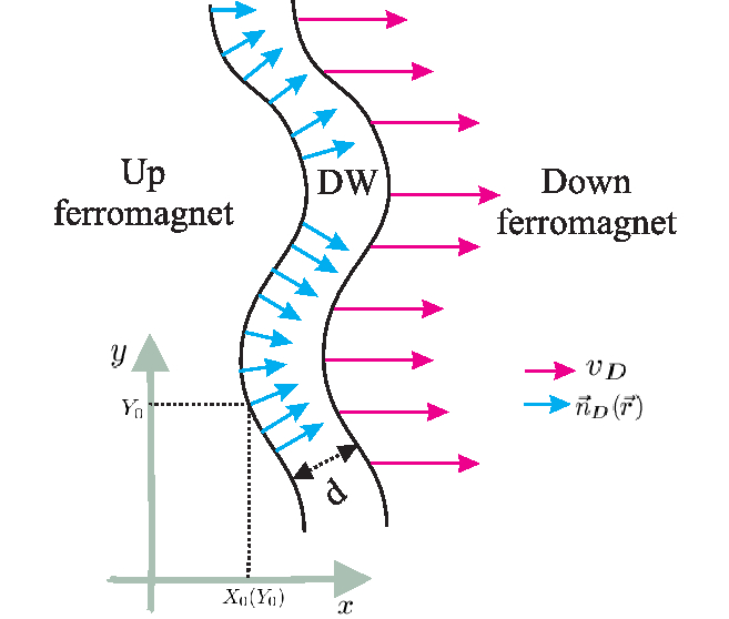
Figure 1: A typical form of the deformed DW in the real space. DW has been placed between two oppositely directed magnetic domains. A Bloch-type DW has been considered in which the DW rotation axis located in the plane of the system. The bulging of the DW can be formulated if we consider that the DW rotation axis is always vertically oriented to the DW boundaries. $n_{D}$ denotes the DW rotation axis while $v_{D}$ indicates the speed of the DW and $d$ is the DW width.

If we restrict ourself to the case of the two-dimensional DWs i.e. when ($n_{Dz}=0$) we obtain the simplest case of two dimensional bulging as follows

$$\vec{n}(\vec{r}) = -n_{Dy}\sin(\theta(X_{D}))\hat{x}$$ (37)

$$+n_{Dx}\sin(\theta(X_{D}))\hat{y}+\cos(\theta(X_{D}))\hat{z}.$$

DW width has been assumed to be locally constant during the DW rigid motion. The DW motion has been considered as a successive switching of the local spins that as mentioned before. In the case of the rigid DW motion it was assumed that the spin switching time is very short and a localized spin switches abruptly without precession. Meanwhile it was assumed that the DW rigidly moves along the $x$ axis. Since in this case we can write

$$\phi(y)=tan^{-1}(-n_{Dy}(y)/n_{Dx}(y))=-\phi_{D}$$ (38)

and

$$X_{D}(r,t) = \vec{n}_{D}\cdot\vec{r}$$

$$= n_{Dx}(x-X_{0}(Y_{0})-v_{D}t)+n_{Dy}(y-Y_{0})$$

where $X_{0}(Y_{0})$ is the left boundary of the DW at the initial time. This curved boundary preserves its shape during the DW motion which sweeps and removes the downward ferromagnetic region (right region in Fig. 1) during the motion of the DW.

The space time Berry curvature is given by

$$\Omega_{yt} = \Omega_{\theta\phi}(\partial_{y}\phi)(\partial_{t}\theta(X_{D}))$$

$$= \Omega_{\theta\phi}n_{Dx}v_{D}\partial_{X_{D}}\theta(X_{D}))(n_{Dx}\partial_{y}n_{Dy}-n_{Dy}\partial_{y}n_{Dx}).$$

Since we can write $n^{2}_{Dx}+n^{2}_{Dy}=1$, therefore

$$n_{Dx}(n_{Dx}\partial_{y}n_{Dy}-n_{Dy}\partial_{y}n_{Dx})=\partial_{y}n_{Dy}$$ (41)

Meanwhile in the absence of the Rashba interaction we have $\beta=\phi$ and $\cos\gamma=\cos\theta$ and therefore $\Omega_{\theta\phi}=1/2\sin(\theta)$. Accordingly

$$\Omega_{yt}=\frac{\pi}{4d}\sin(\theta(X_{D}))v_{D}\cosh^{-2}(X_{D}/d)\partial_{y}n_{Dy}$$ (42)

and similarly we can obtain

$$\Omega_{xt}=\frac{\pi}{4d}\sin(\theta(X_{D}))v_{D}\cosh^{-2}(X_{D}/d)\partial_{x}n_{Dy}.$$ (43)

Unlike the straight DWs in which the electromotive force could only generated as a result of the precession, regardless of the DW motion, in the current case for deformed DWs we have shown that the electromotive force could be generated along the direction of motion and even normal to this direction.

It should be considered that the averaged electromotive force along the direction of the DW motion could vanish identically when the DW curve has mirror symmetry and the direction of the DW speed is parallel to the plane of mirror symmetry. Meanwhile, even in this case the normal electromotive force still survives and the rigid DW motion could generate an electromotive force normal to the direction of motion i.e. perpendicular to the mirror symmetry plane. Therefore the electromotive force induced by the rigid motion of the domain wall can identically vanish when the domain wall has two vertical mirror symmetry planes. However in this case the domain wall should be formed as a closed symmetric curve i.e. one of the magnetic domains should be surrounded by its opposite counterpart.

Without loss of generality we can assume that the domain wall motion is along the x direction. If we assume that the $xz$ plane is the mirror plane of the DW therefore $X_{0}(-Y_{0})=X_{0}(Y_{0})$, $n_{Dx}(x,-y)=n_{Dx}(x,y)$ and $n_{Dy}(x,-y)=-n_{Dy}(x,y)$. Therefore $X_{D}$ remains unchanged under the coordinate change: $y\rightarrow-y$ and $Y_{0}\rightarrow-Y_{0}$. In this case since $\Omega_{xt}$ is an odd function of $y$ the spatial average of the electromotive force along the direction of the DW motion, $(-\hbar/eL)\int_{S}dxdy\Omega_{xt}$, vanishes identically. Where the integration has been performed over the DW area which has been specified by $S$ and $L$ is the length of the DW. Meanwhile in the normal direction $\Omega_{yt}$ is an even function and the averaged electromotive force, $(-\hbar/eL)\int_{S}dxdy\Omega_{yt}$, cannot vanish simultaneously. Finally we can conclude that electromotive force induced by the rigid DW motion cannot go all the way to zero for any arbitrary open curved DWs.

It should be noted that in the previous studies in this filed Volovik ; PhysRevLett.102.086601 ; PhysRevLett.107.236602 spin-motive force was shown to be proportional to $|\partial\textbf{m}/\partial t\times\partial\textbf{m}/\partial x|$. Since in the precession-less limit $\partial\textbf{m}/\partial t$ identically vanishes, this means that the zeroth order spin-motive force is zero for rigid motion of the DW. Meanwhile if we consider the perturbative induced effects in the effective field of the system, perturbative terms of $\partial\textbf{m}/\partial t$ could be non-zero and accountable. Spatially non-homogeneous magnetization results in effective magnetic field on conduction electrons given by $\textbf{B}_{i}\sim\epsilon^{ijk}(\partial_{j}\textbf{m}\times\partial_{k}\textbf{m})\cdot\textbf{m}$. Since the spin torque on the local magnetization is the opposite of the torque exerted on the conduction electrons. Therefore local magnetization even in the precession-less limit has time evolution PhysRevLett.102.086601 .

4 Conclusion

In the current study we have developed the Berry curvature based theory of the DW electromotive force for the deformed DWs. In the previous studies it has been demonstrated that for straight DWs rigid motion of the DW could not contribute in the ferro-Josephson effect MacDonald . In the other words this type of domain wall dynamics which takes place below the Walker field could not generate electromotive force and the spin precession plays the central role in the electromotive force generation MacDonald . However in the current study we have demonstrated that this is not the case for the deformed DWs. It has been shown that the DW bulging results in effective electromotive force in the case of rigid the motion of the domain wall. In addition we have shown that the generated electromotive force could be either along the DW motion axis or in the transverse direction.

References

- (1) M.V. Berry, in Proceedings of the Royal Society of London A: Mathematical, Physical and Engineering Sciences, vol. 392 (1984), vol. 392, pp. 45–57
- (2) D. Xiao, M.C. Chang, Q. Niu, Rev. Mod. Phys. 82(3), 1959 (2010)
- (3) F. Wilczek, A. Shapere, Geometric phases in physics, vol. 5 (World Scientific Singapore, 1989)
- (4) A. Böhm, H. Koizumi, Q. Niu, J. Zwanziger, A. Mostafazadeh, The geometric phase in quantum systems (Springer, 2003)
- (5) N. Nagaosa, J. Sinova, S. Onoda, A. MacDonald, N. Ong, Rev. Mod. Phys. 82(2), 1539 (2010)
- (6) I. Turek, J. Kudrnovskỳ, V. Drchal, Phys. Rev. B 86(1), 014405 (2012)
- (7) J. Weischenberg, F. Freimuth, J. Sinova, S. Blügel, Y. Mokrousov, Phys. Rev. Lett. 107(10), 106601 (2011)
- (8) S. Lowitzer, D. Koedderitzsch, H. Ebert, Phys. Rev. Lett. 105(26), 266604 (2010)
- (9) X. Wang, J.R. Yates, I. Souza, D. Vanderbilt, Phys. Rev. B 74(19), 195118 (2006)
- (10) Y. Yao, L. Kleinman, A. MacDonald, J. Sinova, T. Jungwirth, D.s. Wang, E. Wang, Q. Niu, Phys. Rev. Lett. 92(3), 037204 (2004)
- (11) A. Neubauer, C. Pfleiderer, B. Binz, A. Rosch, R. Ritz, P. Niklowitz, P. Böni, Phys. Rev. Lett. 102(18), 186602 (2009)
- (12) N. Kanazawa, Y. Onose, T. Arima, D. Okuyama, K. Ohoyama, S. Wakimoto, K. Kakurai, S. Ishiwata, Y. Tokura, Phys. Rev. Lett. 106(15), 156603 (2011)
- (13) S. Mühlbauer, B. Binz, F. Jonietz, C. Pfleiderer, A. Rosch, A. Neubauer, R. Georgii, P. Böni, Science 323(5916), 915 (2009)
- (14) S. Huang, C. Chien, Phys. Rev. Lett. 108(26), 267201 (2012)
- (15) G. Sundaram, Q. Niu, Physical Review B 59(23), 14915 (1999)
- (16) A. Stern, Phys. Rev. Lett. 68(7), 1022 (1992)
- (17) S. Barnes, S. Maekawa, Phys. Rev. Lett. 98(24), 246601 (2007)
- (18) S.A. Yang, G.S.D. Beach, C. Knutson, D. Xiao, Z. Zhang, M. Tsoi, Q. Niu, A.H. MacDonald, J.L. Erskine, Phys. Rev. B 82, 054410 (2010)
- (19) Y. A, O. T, N. S, M. K, M. K, S. T, Phys. Rev. Lett. 92, 077205 (2004)
- (20) T. Gen, K. Hiroshi, Phys. Rev. Lett. 92, 086601 (2004)
- (21) L. Berger, Phys. Rev. B 33, 1572 (1986)
- (22) S.A. Yang, G.S. Beach, C. Knutson, D. Xiao, Q. Niu, M. Tsoi, J.L. Erskine, Phys. Rev. Lett. 102(6), 067201 (2009)
- (23) W.M. Saslow, Phys. Rev. B 76, 184434 (2007)
- (24) R.A. Duine, Phys. Rev. B 77, 014409 (2008)
- (25) N.L. Schryer, L.R. Walker, J. Appl. Phys. 45, 5406 (1974)
- (26) M. Nakahara, Geometry, topology and physics (CRC Press, 2003)
- (27) G.E. Volovik, Journal of Physics C: Solid State Physics 20(7), L83
- (28) S. Zhang, S.S.L. Zhang, Phys. Rev. Lett. 102, 086601 (2009)
- (29) Y. Yamane, K. Sasage, T. An, K. Harii, J. Ohe, J. Ieda, S.E. Barnes, E. Saitoh, S. Maekawa, Phys. Rev. Lett. 107, 236602 (2011)