Abstract

In many situations, in all branches of physics, one encounters power-like behavior of some variables which are best described by a Tsallis distribution characterized by a nonextensivity parameter $q$ and scale parameter $T$. However, there exist experimental results which can be described only by a Tsallis distributions which are additionally decorated by some log-periodic oscillating factor. We argue that such a factor can originate from allowing for a complex nonextensivity parameter $q$. The possible information conveyed by such an approach (like the occurrence of complex heat capacity, the notion of complex probability or complex multiplicative noise) will also be discussed.

10.3390/—— xx Received: xx / Accepted: xx / Published: xx Tsallis Distribution Decorated With Log-Periodic Oscillation Grzegorz Wilk^1,*, Zbigniew Włodarczyk² wilk@fuw.edu.pl, +48-22-621 60 85

1 Introduction

In many situations, in all branches of physics, one encounters behavior of some variables $X$ which become pure power distributions for large values of $X$ and exponential for $X\rightarrow 0$. Because of this they are known as power-like distributions and in many cases they are identified with a Tsallis distribution Tsallis ,

$$F(X)=A~{}\left[1-\left(1-q\right)\frac{X}{T}\right]^{1/(1-q)},$$ (1)

characterized by a scale parameter $T$ and parameter $q$ known as nonextensivity parameter ($A$ is normalization). Obviously, for $X\rightarrow 0$ distribution (1) becomes the usual Boltzmann-Gibbs exponential formula with temperature $T$, but it becomes pure exponential (i.e., BG) also for $q\rightarrow 1$. For $q\neq 1$ and large values of $X$ it becomes pure power distribution not sensitive to scale parameter $T$.

To fully recognize the nontrivial character of distribution (1), one must realize that, usually, in different parts of phase space of the variable $X$, one encounters (or, rather, one expects) a dominance of different (if not completely disparate) dynamical factors. This is best seen in the processes of multiparticle production at high energies (the best known to us). They will serve here to exemplify our further consideration concerning some specific log-periodic oscillations, apparently visible in such processes, which must be therefore somehow hidden in the original distribution (1).

Before proceeding further, we shall briefly summarize the present status of application of Tsallis distributions in this context, concentrating only on multiparticle production processes. They comprise of many different mechanisms in different parts of phase space. Limiting ourselves only to particle production in the central rapidity region and to distribution of their transverse momenta $p_{T}$, it is customary to divide this production into independent soft and hard processes populating different parts of the transverse momentum space separated by a momentum scale $p_{0}$. As a rule of thumb, the spectra of the soft processes in the low-$p_{T}$ region are (almost) exponential, $F(p_{T})$$\sim$$\exp(-p_{T}/T)$, and are usually associated with the thermodynamical description of the hadronizing system. The $p_{T}$ spectra of the hard process in the high-$p_{T}$ region are regarded as essentially power-like, $F(p_{T})$$\sim$$p_{T}^{-n}$, and are usually associated with the hard scattering process (for relevant literature concerning both parts see ISMD2014 ). However, it was very soon recognized that both descriptions could be replaced by a simple interpolating formula Michael ,

$$F(p_{T})=A\left(1+\frac{p_{T}}{p_{0}}\right)^{-n},$$ (2)

that becomes power-like for high $p_{T}$ and exponential-like for low $p_{T}$. The reasoning was that for high $p_{T}$, where we are usually neglecting the constant term, the scale parameter $p_{0}$ becomes irrelevant, whereas for low $p_{T}$ it becomes, together with the power index $n$, an effective temperature $T=p_{0}/n$. The same formula re-emerged later to become known as the QCD-based Hagedorn formula H . It was used for the first time in UA1 and became one of the standard phenomenological formulas for $p_{T}$ data analysis PHENIX ; STAR ; CMS ; ATLAS ; ALICE . In the mean time it was realized that both formulas are, in fact, identical once

$$n=\frac{1}{q-1}\quad{\rm and}\quad p_{0}=nT,$$ (3)

and therefore they can be used interchangeably

This distribution is usually used in a thermodynamical content in which the scale parameter $T$ is identified with the usual temperature (although such identification cannot be solid RGC ) and with a real power index $n=1/(q-1)$ (or real nonextensivity parameter $q$). Actually, a Tsallis distribution can be regarded as a generalization to real power $n$ (or $q$) of such well known distributions as the Snedecor distribution (with $n=(\nu+2)/2$ and integer $\nu$, which for $\nu\rightarrow\infty$ it becomes exponential distribution).

In LPOWW we investigate the case when $q$ is a complex number. We shall review our results in this field in the next section adding examples where log-periodic oscillations occur at different energies and for different collision systems. In Section 3 we discuss the possible consequences of complex nonextensivity parameter including some new recent developments in this field (as complex probability and complex multiplicative noise). The final section contains our conclusions and summary.

2 Log-periodic oscillations in Tsallis distribution - complex power index

Recently, the experiments CMS ; ATLAS ; ALICE at the Large Hadron Collider (LHC) at CERN provided new data in a very large domain of transverse momenta, $p_{T}$, phase space. They turned out to be extremely interesting because of the following:

• They allow us to test the standard Tsallis formula, Eq. (1), over $\sim 14$ orders of magnitude. As can be seen in Fig. 1a, the observed $p_{T}$ distributions of secondaries produced in proton-proton collisions in these experiments can be very well reproduced (cf. also CYW .

• And, what is of special importance to us, they disclose some features which suggest a departures from the single form of Eq. (1), cf.Figs. 1 b-c.. Apparently they could not be seen in previous experiments because they seem to be connected with rather large values of transverse momenta, not available earlier..

However, whereas fits to Eq. (1) look pretty good, closer inspection shows that the ratio of data/fit is not flat. It shows some kind of visible oscillations, cf. Fig. 1b. These are the oscillations we have mentioned before.

It turns out that these oscillations cannot be compensated, or erased, by any reasonable change of fitting parameters. Moreover, they are visible by all three experiments CMS, ATLAS, ALICE. The only condition for such an effect to be visible is that the experiment covers a sufficiently large domain of transverse momenta $p_{T}$, cf. Fig. 1b. It is also seen at all energies covered by these experiments, cf. Fig. 1c. And, finally, as Fig. 1d shows, this effect is also visible (and is even more pronounced) in nuclear collisions. When taken seriously, it turns out that to account for these oscillations one has to "decorate" distribution $f\left(p_{T}\right)$ from Eq. (1) (i.e., one has to multiply it) with some log-periodic oscillating factor. It is is usually taken in the form Scaling :

$$R(E)=a+b\cos\left[c\ln(E+d)+f\right].$$ (4)

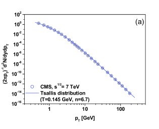
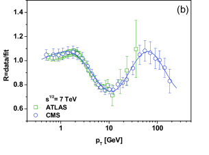
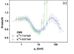
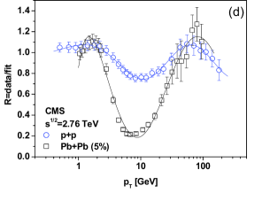
Figure 1: (Color online) Examples of log-periodic oscillations. $(a)$ $dN/dp_{T}$ for highest energy $7$ TeV, the Tsallis behavior is evident. Only CMS data are shown CMS , others behave essentially in an identical manner. $(b)$ Log-periodic oscillations showing up in different experimental data like CMS CMS or ATLAS ATLAS taken at $7$ TeV. $(c)$ Results from CMS CMS for different energies. $(d)$ Results for different systems ($p+p$ collisions compared with $Pb+Pb$ taken for $5$ % centrality CMSPb . Results from ALICE ALICEPb are very similar. Fits for $p+p$ collision at $7,~{}2.76$ and $0.9$ TeV are performed with $q=1.139+i\cdot 0.0385,~{}~{}1.134+i\cdot 0.0269$ and $1.117+i\cdot 0.0307$, respectively. Fit for central $Pb+Pb$ collisions at $2.76$ TeV is done with $q=1.135+i\cdot 0.0321$. See text for more details.

Before proceeding any further let us remember that such log-periodic oscillations are widely know in all situations in which one encounters power distributions. In fact, such behavior has been found in earthquakes EQ , escape probabilities in chaotic maps close to crisis CHM , biased diffusion of tracers on random systems BD , kinetic and dynamic processes on random quenched and fractal media RQFM , when considering the specific heat associated with self-similar VMdST or fractal spectra TdSMVM , diffusion-limited-aggregate clusters DLM , growth models GM , or stock markets near financial crashes FM , to name only a few examples. However, in all these cases the basic distributions were scale free power law, without any scale parameter (here $T$) and without a constant term governing their $X<nT$ behavior.

In the context of nonextensive statistical mechanics log-periodic oscillations have first been observed and discussed while analyzing the convergence dynamics of $z$-logistic maps UT . In this paper we shall propose another way of introducing such oscillations to Tsallis distributions. It will be based on allowing the power index $n$ (or nonextensivity parameter $q$) in a Tsallis distribution to become complex. For completeness of the presentation we start from the simple pure power law distribution,

$$O\left(x\right)=C\cdot x^{-m}.$$ (5)

This function is scale invariant, i.e.,

$$O\left(\lambda x\right)=\mu O\left(x\right),$$ (6)

with $m=-\ln{\mu}/\ln{\lambda}$. However, because $1=\exp{\left(\imath 2\pi k\right)}$, one can as well write that

$$\mu\lambda^{m}=1=\exp{\left(\imath 2\pi k\right)},\quad k=0,1,\dots.$$ (7)

It means therefore that, in general, the index $m$ can become complex,

$$m=-\frac{\ln\mu}{\ln\lambda}+\imath\frac{2\pi k}{\ln\lambda}.$$ (8)

As will be obvious from further, general considerations, such a form of the power index results in $R$ as given by Eq. (4) when one only keeps $k=0,1$ terms (which is the usual assumption customary applied in all applications Scaling ; EQ ; CHM ; BD ; RQFM ).

However, Tsallis distribution is only a power-like, not a power distribution. Therefore, to explain the origin of such a dressing factor in this case one has to find a right variable in which the real scaling holds. We start from the observation that, whereas the Boltzmann-Gibbs (BG) distribution,

$$f(E)=\frac{1}{T}\exp\left(-\frac{E}{T}\right),$$ (9)

comes from the simple equation,

$$\frac{df(E)}{dE}=-\frac{1}{T}f(E),$$ (10)

with the scale parameter $T$ being constant, the same equation, but with variable scale parameter in the form

$$T=T(E)=T_{0}+\frac{E}{n},$$ (11)

(known as preferential attachment in networks NETWORKS ; qWW1 ),

$$\frac{df(E)}{dE}=-\frac{1}{T(E)}f(E)=-\frac{1}{T_{0}+E/n}f(E),$$ (12)

results in the Tsallis distribution

$$f(E)=\frac{n-1}{nT_{0}}\left(1+\frac{E}{nT_{0}}\right)^{-n}.$$ (13)

We shall write now Eq. (12) in finite difference form,

$$f(E+\delta E)=\frac{-n\delta E+nT+E}{nT+E}f(E).$$ (14)

In practical sense this means a first-order Taylor expansion for small $\delta E<<E$ (from Eq. (14) on, we use $T$ instead of $T_{0}$). We shall now consider a situation in which $\delta E$ always remains finite (albeit, depending on the value of the new scale parameter $\alpha$, it can be very small) and equal to

$$\delta E=\alpha nT(E)=\alpha(nT+E).$$ (15)

Because one expects that changes $\delta E$ are of the order of the temperature $T$, the scale parameter must be limited by $1/n$, i.e., $\alpha<1/n$. In this case, substituting (15) into (14), we have,

$$f[E+\alpha(nT+E)]=(1-\alpha n)f(E).$$ (16)

Expressing Eq. (16) in a new variable $x$,

$$x=1+\frac{E}{nT},$$ (17)

we recognize that the argument of the function on the left-hand side of equality (16) is

$$E+\alpha(nT+E)=(1+\alpha)xnT-nT,$$

while the argument of the function on its right-hand side is

$$E=xnT-nT.$$

Notice that, in comparison with the right-hand side, the variable $x$ on the left-hand side is multiplied by the additional factor $(1+\alpha)$. This means that, formally, Eq.(16), when expressed in $x$, corresponds to the following scale invariant relation:

$$g[(1+\alpha)x]=(1-\alpha n)g(x).$$ (18)

This means than that, following the discussion after Eq. (6), its general solution is a power law,

$$g(x)=x^{-m_{k}},$$ (19)

with exponent $m_{k}$ depending on $\alpha$ and acquiring an imaginary part,

$$m_{k}=-\frac{\ln(1-\alpha n)}{\ln(1+\alpha)}+ik\frac{2\pi}{\ln(1+\alpha)}.$$ (20)

The special case of $k=0$, i.e., the usual real power law solution with $m_{0}$ corresponding to fully continuous scale invariance, recovers in the limit $\alpha\rightarrow 0$ the power $n$ in the usual Tsallis distribution. In general one has

$$g(x)=\sum_{k=0}w_{k}\cdot{\rm Re}\left(x^{-m_{k}}\right)=x^{-{\rm Re}\left(m_{k}\right)}\sum_{k=0}w_{k}\cdot\cos\left[{\rm Im}\left(m_{k}\right)\ln(x)\right].$$ (21)

One therefore obtains a Tsallis distribution decorated by a weighted sum of log-oscillating factors (where $x$ is given by Eq. (17)). Because usually in practice we do not a priori know the details of the dynamics of processes under consideration (i.e., we do not known the weights $w_{k}$), for fitting purposes one usually uses only $k=0$ and $k=1$. In this case one has, approximately,

$$g(E)\simeq\left(1+\frac{E}{nT}\right)^{-m_{0}}\left\{w_{0}+w_{1}\cos\left[\frac{2\pi}{\ln(1+\alpha)}\ln\left(1+\frac{E}{nT}\right)\right]\right\}$$ (22)

and reproduces the general form of a dressing factor given by Eq. (4) and often used in the literature Scaling . In this approximation the parameters $a$, $b$, $c$, $d$ and $f$ from Eq. (4) get the following meaning:

$$\frac{a}{b}=\frac{w_{0}}{w_{1}},\qquad c=\frac{2\pi}{\ln(1+\alpha)},\qquad d=nT,\qquad f=-\frac{2\pi}{\ln(1+\alpha)}\ln(nT).$$ (23)

In fact this is not the most general result for in our derivation, Eqs.(15)-(18)), we have so far only accounted for a single step evolution. In real situation one should expect to have a whole hierarchy of evolutions. In such a case consecutive steps of evolution are connected by:

$$E_{i}=E_{i-1}+\alpha_{i-1}\left(nT+E_{i-1}\right),$$ (24)

each with its own scale parameter $\alpha_{i}$. In the simplest situation, neglecting any fluctuations of consecutive scaling parameters, i.e., assuming that all $\alpha_{i}=\alpha$, one has that after $\kappa$ steps

$$nT+E_{\kappa}=(1+\alpha)^{\kappa}\left(nT+E_{0}\right).$$ (25)

This means that, in general, Eq. (18) should be replaced by a new scale invariant equation:

$$g\left[(1+\alpha)^{\kappa}x\right]=(1-\alpha n)^{\kappa}g(x).$$ (26)

Whereas this equation does not change the slope parameter $m_{0}$, it significantly influences the frequency of oscillations which are now $\kappa$ times smaller,

$$c=\frac{2\pi}{\kappa\ln(1+\alpha)}$$ (27)

(in Eq.(26) $\lambda=(1+\alpha)^{\kappa}$ and $\mu=(1-\alpha n)^{\kappa}$; the slope parameter $m_{0}=-\ln\mu/\ln\lambda$ is independent of $\kappa$, whereas the frequency of oscillations, $2\pi/\ln\lambda$, decreases with $\kappa$ as $1/\kappa$). For more complex behavior of intermediate scale parameters $\alpha_{i}$ one gets more complicated expressions (we shall not discuss this here).

3 Other consequences of complex nonextensivity parameter

There are other consequences of allowing the parameter $m$ to be complex. In what follows we shall discuss shortly three examples: complex heat capacity , complex probability and complex multiplicative noise.

3.1 Complex heat capacity

The complex power exponent in the Tsallis distribution, $m=m^{\prime}+i\cdot m^{\prime\prime}$, means that

$$q-1=\frac{1}{m}=\frac{m}{|m|^{2}}^{\prime}+i\frac{m^{\prime\prime}}{|m|^{2}}.$$ (28)

As shown in BiroC (cf. also Cq ; qWW1 ; qWW ), the nonextensivity parameter $q$ can be treated as a measure of the thermal bath heat capacity $C$ with

$$C=\frac{1}{q-1}=m^{\prime}+im^{\prime\prime}.$$ (29)

The complex nonextensive parameter $q$ must therefore have some profound consequences because now the corresponding heat capacity becomes complex as well. As a matter of fact, such complex (frequency dependent) heat capacities (or generalized calorimetric susceptibilities) are known in the literature HC and are usually written in the form

$$C=C_{\infty}+\frac{C_{0}-C_{\infty}}{1+(\omega\tau)^{2}}(1-i\omega\tau).$$ (30)

Here $C_{\infty}$ is the heat capacity related to the infinitely fast degrees of freedom of the system as compared to the frequency $\omega$, and $C_{0}$ is the total contribution at equilibrium (the frequency is set to zero) of the degrees of freedom, fast and slow, of the sample. The time constant $\tau$ is the kinetic relaxation time constant of a certain internal degree of freedom.

These complex heat capacities are known as dynamic heat capacities and are intensively explored from both experimental and theoretical perspectives. It is expected that dynamic calorimetry can provide an insight into the energy landscape dynamics, cf., for example, G2007 ; GR2007 ; ND ; S . Usually one associates the imaginary part of linear susceptibility with the absorption of energy by the sample from the applied field.

In the case of temperature fluctuations $\delta T(t)$ the deviation of the energy from its equilibrium value $\delta U(t)$ is, for a certain linear operator $\hat{C}(t)$, some linear function of the corresponding variation of the temperature,

$$\delta U(t)=\hat{C}\delta T(t).$$ (31)

If the temperature of the reservoir changes infinitely slowly in time, then the system can keep up with any changes in the reservoir and its susceptibility is just the specific heat of the system $C_{V}$. However, in general, the behavior of the system is described by a generalized susceptibility $C_{V}(\omega)$, which can be called the complex and $\omega$-dependent heat capacity of the system. The change in the energy of a system in the field of the thermal force can be represented by

$$\delta U(t)=\int L\left(t^{\prime}\right)\delta T\left(t-t^{\prime}\right)dt^{\prime},$$ (32)

where $L\left(t^{\prime}\right)$ is the response function of the system describing its relaxation properties given by $\Phi(t)=\int_{t}^{\infty}L\left(t^{\prime}\right)dt^{\prime}$. Taking the Fourier transform one gets

$$\delta U(\omega)=C_{V}(\omega)\delta T(\omega),$$ (33)

where

$$C_{V}(\omega)=\int L\left(t^{\prime}\right)e^{i\omega t^{\prime}}dt^{\prime}$$ (34)

is the generalized susceptibility of the system and is called the complex heat capacity. In practice, the frequency dependent heat capacity is a linear susceptibility describing the response of the system to the small thermal perturbation (occurring on the time scale $1/\omega$) that takes the system slightly away from the equilibrium .

A complex $C_{V}(\omega)$ means that $\delta U$ and $\delta T$ are shifted in phase and that the entropy production in the system differs from zero S . The corresponding fluctuation-dissipation theorem for the frequency dependent heat capacity was established in ND . According to this result, the frequency-dependent heat capacity may be expressed within the linear response approximation as a linear susceptibility describing the response of the system to arbitrarily small temperature perturbations away from equilibrium,

$$C_{V}(\omega)=\frac{\langle U^{2}\rangle_{0}}{\langle T\rangle^{2}}\,-\,i\frac{\omega}{\langle T\rangle^{2}}\int_{0}^{\infty}dte^{-i\omega t}\langle U(0)U(t)\rangle$$ (35)

(the $\omega$ denotes frequency with which temperature field is varying with time).

The above results for heat capacity can now be used to a new phenomenological interpretation of the complex $q$ parameter discussed before. Namely, one can argue that

$$q-1=\frac{Var(T)}{\langle T\rangle^{2}}-i\,\frac{S(T)}{\langle T\rangle^{2}},$$ (36)

were

$$S(T)=\omega\int Cov[T(0),T(t)]e^{-i\omega t}\,dt$$ (37)

is the spectral density of temperature fluctuations (i.e., the Fourier transform of the covariance function averaging over the nonequilibrium density matrix).

We would like to stress at this point that, in a sense, Eq. (36) can be regarded as a generalization of our old proposition for interpreting $q$ as a measure of nonstatistical intrinsic fluctuations in the system WWB ; SSB (which corresponds to the real part of (36)) by adding the effect of spectral density of such fluctuations (via the imaginary part of (36)). Notice that (36) follows from (29) and the relation $U=C_{V}T$, allowing to write (35) in the form of (36).

3.2 Complex probability

From the point of view of superstatistics SuperS ; WWB , in our particular case complex parameter $q$ corresponds to a complex probability distribution. Namely, one uses the property that gamma-like fluctuation of the scale parameter $T$ in an exponential BG distribution (9) results in the $q$-exponential Tsallis distribution (1) with $q>1$. The parameter $q$ is given here by the strength of these fluctuations, $q=1+Var(X)/<X>^{2}$. From the thermal perspective, it corresponds to situation in which the heath bath is not homogeneous but has different temperatures in different parts, which are fluctuating around some mean temperature $T_{0}$. It must be therefore described by two parameters: a mean temperature $T_{0}$ and the mean strength of fluctuations given by $q$.

We now perform the same procedure, but using two gamma distributions, one with a real power index, $m_{0}-1$, and one with a complex power index, $m_{0}+im_{1}-1$,

$$g(1/T) = w_{0}\frac{1}{\Gamma\left(m_{0}\right)}nT_{0}\left(n\frac{T_{0}}{T}\right)^{m_{0}-1}\exp\left(-n\frac{T_{o}}{T}\right)+$$ (38)

$$+w_{1}\frac{1}{\Gamma\left(m_{0}+im_{1}\right)}nT_{0}\left(n\frac{T_{0}}{T}\right)^{m_{0}+im_{1}-1}\exp\left(-n\frac{T_{0}}{T}\right).$$

As the result one gets a complex distribution (complex pdf):

$$h_{q}(E)=\int_{0}^{\infty}\,f(E)g(1/T)d(1/T)=Cw_{0}\left(1+\frac{E}{nT_{0}}\right)^{-m_{0}}+Cw_{1}\left(1+\frac{E}{nT_{0}}\right)^{-m_{0}-im_{1}},$$ (39)

the real part of which is pdf in form of a Tsallis distribution decorated with log-periodic oscillations of the type of Eq. (22),

$$Re\left[h_{q}(E)\right]=C\left(1+\frac{E}{nT_{0}}\right)^{-m_{0}}\cdot\left\{w_{0}+w_{1}\cos\left[m_{1}\ln\left(1+\frac{E}{nT_{0}}\right)\right]\right\}.$$ (40)

The complex pdf has a number of interesting properties HB ; MZ . It plays an important role in the interference among resonance states during scattering experiments. It is associated with the phase of the resonance channel probability amplitudes (in non-Hermitian quantum mechanics). In wireless communication systems it is generated by a superposition of finite random variables and usually involves the movement, scattering, diffusion or diffraction. The imaginary part is proportional to the degree of the correlation. The imaginary part is then a function of a correlation coefficient or other parameters that state the degree of the relationship of each individual random variable of the superposition of the random variable having a complex pdf. The real and imaginary part have diverse properties, i.e. one for real valued pdf and the other for elementary correlation, respectively.

It is interesting to note that entropy

$$H=-\left|\int\int(a\ln a+i\cdot b\ln b)dx_{1}dx_{2}\right|=$$ (41)

corresponding to complex joint probability,

$$f\left(x_{1},x_{2}\right)=a\left(x_{1},x_{2}\right)+i\cdot b\left(x_{1},x_{2}\right),$$ (42)

consists of two components:

$$\!\!H_{1}=-\int\!\!\int a\ln a\,dx_{1}dx_{2},\quad H_{2}=-\int\!\!\int b\ln b\,dx_{1}dx_{2};\quad H=\left|H_{1}+iH_{2}\right|\sqrt{H_{1}^{2}+H_{2}^{2}}\geq H_{1}.$$ (43)

The imaginary part of entropy is proportional to the degree of incompatibility of the correlated stochastic processes. The incompatibility increases the entropy of correlated stochastic processes.

3.3 Complex multiplicative noise

It is known that multiplicative noise leads to a Tsallis distribution SSB . It is then natural to expect that multiplicative complex noise should result in complex $q$ and in log-periodic oscillations in Tsallis distributions. It can be defined by a Langevin equation

$$\frac{dp}{dt}+\gamma(t)p=\xi(t),\quad{\rm where}\quad\gamma(t)=\gamma_{0}(t)+i\gamma_{1}.$$ (44)

The resulting distribution SSB is now

$$f(p)=\left(1+\frac{q-1}{T}p^{2}\right)^{\frac{q}{q-1}}\quad{\rm where}\quad T=\frac{2Var(\xi)}{\langle\gamma\rangle},\quad q=1+\frac{2Var(\gamma)}{\langle\gamma\rangle}.$$ (45)

The parameter $q$ is now complex because $\langle\gamma\rangle$ is complex. Even more importantly, $(q-1)/T=Var(\gamma)/Var(\xi)$ is real (it tends to zero for $q\rightarrow 1$). This is because the complex term $\gamma_{1}$ added to the noise is constant. Notice that we could just as well replace in Eq. (45) $(q-1)\left(p^{2}/T\right)$ by $\left(p^{2}/p_{0}^{2}\right)$ where $p_{0}^{2}=Var(\xi)/Var(\gamma)$. The examples and discussion of the systems characterized by the appearance of "imaginary" multiplicative noise terms in an effective Langevin-type description can be found in CLang .

4 Summary and conclusions

In may places in physics, and especially in the realm of high energy multiparticle production processes we are particularly interested in, it became a standard procedure to fit the data on transverse momentum distributions by means of the quasi-power Tsallis formula. The usual interpretation in such cases is that the scale parameter $T$ is a kind of "temperature" whereas additional nonextensivity parameter $q$ is describes intrinsic, nonstatistical fluctuations existing in the system BCM ; Beck ; RWW ; qWW1 ; qWW ; Wibig ; Biro ; BiroC ; JCleymans ; ADeppman ; Others ; WalRaf ; qCR ; SuperS ; WWB ; SSB ; RodosWW . However, with increasing range of transverse momenta measured in recent experiments CMS ; ATLAS ; ALICE two things happened:

• That they still can be fitted by the same formula (which came as surprise because fits now cover $\sim 14$ orders of magnitude of the measured cross sections CYW ; ISMD2014 ).

• That new data revealed weak but persistent oscillation of log-periodic character (discussed already shortly in LPOWW ).

If taken seriously, such log-periodic structures in the data indicate that the system and/or the underlying physical mechanisms have characteristic scale invariant behavior. This is interesting as it provides important constraints on the underlying physics. The presence of log-periodic features signals the existence of important physical structures hidden in the fully scale invariant description. It is important to recognize that Eq. (12) represents an averaging over highly ’non-smooth’ processes and, in its present form, suggests rather smooth behavior. In reality, there is a discrete time evolution for the number of steps. To account for this fact, one replaces a differential Eq. (10) by a difference quotient and expresses $dt$ as a discrete step approximation given by Eq. (15) with parameter $\alpha$ being a characteristic scale ratio. It can also be shown that discrete scale invariance and its associated complex exponents can appear spontaneously, without a pre-existing hierarchical structure. Finally, a complex nonextensivity parameter promises new perspectives in future phenomenological applications being connected to complex heat capacity, to notion of complex probability or to complex multiplicative noise, to mention only a few examples discussed shortly in our paper.

- (1) Tsallis, C. Possible generalization of Boltzman-Gibbs statistics. J. Statist. Phys. 1998 52 479-487. Tsallis, C. Nonadditive entropy: The concept and its use. Eur. Phys. J. A 2009 40 257-266. Tsallis, C. Introduction to Nonextensive Statistical Mechanics (Springer, 2009). For an updated bibliography on this subject, see http://tsallis.cat.cbpf.br/biblio. htm.
- (2) Wong, C.-Y.; Wilk, G.; Cirto, L.J.L.; Tsallis, C. Possible Implication of a Single Nonextensive Distribution for Hadron Production in High-Energy pp Collisions. arXiv:1412.0474[hep-ph]; presented at the XLIV International Symposium on Multiparticle Dynamics; 8 - 12 September 2014 - Bologna, ITALY; to be published in EPJ Web of Conferences 2015.
- (3) Michael, G.; Vanryckeghem, L. Consequences of momentum conservation for particle production at large transverse momentum. J. Phys. G 1977 3 L151-L156. Michael, C. Large transverse momentum and large mass production in hadronic interactions. Prog. Part. Nucl. Phys. 1979 2 1-39.
- (4) Hagedorn, R. Multiplicities, distributions and the expected hadron quark-gluon phase transition. Riv. Nuovo Cimento 1983 6 1-50.
- (5) Arnison, G.; et al (UA1 Collab.). Transverse momentum spectra for charged particles at the CERN proton-antiproton collider. Phys. Lett. B 1982 118 167-172.
- (6) Adare, A.; et al. (PHENIX Collaboration). Measurement of neutral mesons in p+p collisions at GeV and scaling properties of hadron production. Phys. Rev. D 2011 83 052004. Adare, A.; et al. (PHENIX Collaboration). Identified charged hadron production in p+p collisions at and 62.4 GeV. Phys. Rev. C 2011 83 064903.
- (7) Adams, J.; et al. (STAR Collaboration). Multiplicity dependence of Multiplicity dependence of inclusive spectra from p-p collisions at GeV. Phys. Rev. D 2006 74 032006.
- (8) Khachatryan, V.; et al. (CMS Collaboration). Transverse-momentum and pseudorapidity distributions of charged hadrons in pp collisions at and TeV. JHEP 2010 02 041. Khachatryan, V.; et al. (CMS Collaboration). Charged particle transverse momentum spectra in pp collisions at and TeV. JHEP 2011 08 086; Khachatryan, V.; et al. (CMS Collaboration).Transverse-Momentum and Pseudorapidity Distributions of Charged Hadrons in pp Collisions at TeV. Phys. Rev. Lett. 2010 105 022002.
- (9) Aad, G.; (ATLAS Collaboration). Charged-particle multiplicities in pp interactions measured with the ATLAS detector at the LHC. New J. Phys. 2011 13 053033.
- (10) Aamodt, K.; et al. (ALICE Collaboration). Transverse momentum spectra of charged particles in proton-proton collisions at GeV with ALICE at the LHC. Phys. Lett. B 2011 693 53-68. Aamodt, K.; et al. (ALICE Collaboration). Strange particle production in proton-proton collisions at with ALICE at the LHC. Eur. Phys. J. C 2011 71 1594.
- (11) Bediaga, I.; Curado, E. M. F.; de Miranda, J. M. A nonextensive thermodynamical equilibrium approach in hadrons. Physica A 2000 286 156-163.
- (12) Beck, C. Non-extensive statistical mechanics and particle spectra in elementary interactions. Physica A 2000 286 164-180.
- (13) Wilk, G.; Włodarczyk, Z. Power laws in elementary and heavy-ion collisions. Eur. Phys. J. A 2009 40 299-312. Rybczyński, M.; Włodarczyk, Z. Tsallis statistics approach to the transverse momentum distributions in p-p collisions. Eur. Phys. J. C 2014 74 2785.
- (14) Wilk, G.; Włodarczyk, Z. Consequences of temperature fluctuations in observables measured in high-energy collisions. Eur. Phys. J. A 2012 48 161.
- (15) Wilk, G.; Włodarczyk, Z. The imprints of superstatistics in multiparticle production processes. Cent. Eur. J. Phys. 2012 10 568-575.
- (16) Wibig, T. The non-extensivity parameter of a thermodynamical model of hadronic interactions at LHC energies. J. Phys. G 2010 37 115009. Wibig, T. Constrains for non-standard statistical models of particle creations by identified hadron multiplicity results at LHC energies. Eur. Phys. J. C 2014 74 2966.
- (17) Ürmösy, K.; Barnaföldi, G.G.; Biró, T.S. Generalised Tsallis statistics in electron-positron collisions. Phys. Lett. B 2011 701 111-116. Ürmösy, K.; Barnaföldi, G.G.; Biró, T.S. Microcanonical jet-fragmentation in proton-proton collisions at LHC energy. Phys. Lett. B 2012 718 125-129. Biró, T.S.; Barnaföldi, G.G.; Van, P. New entropy formula with fluctuating reservoir. Physica A 2015 417 215-220.
- (18) Biró, T.S.; Barnaföldi, G.G.; Van, P. Quark-gluon plasma connected to finite heat bath. Eur. Phys. J. C 2013 49 110.
- (19) Cleymans, J.; Worku, D. The Tsallis distribution in proton-proton collisions at = 0.9 TeV at the LHC. J. Phys. G 2012 39 025006. Cleymans, J.; Worku, D. Relativistic thermodynamics: Transverse momentum distributions in high-energy physics. Eur. Phys. J. A 2012 48 160. Azmi, M.D.; Cleymans, J. Transverse momentum distributions in proton-proton collisions at LHC energies and Tsallis thermodynamics. J. Phys. G 2014 41 065001
- (20) Deppman, A. Properties of hadronic systems according to the nonextensive self-consistent thermodynamics. J. Phys. G 201441 055108. Sena, I; Deppman, A. Systematic analysis of -distributions in collisions. Eur. Phys. J. A 2013 49 17. Marques, L.; Andrade-II, E.; Deppman, A. Nonextensivity of hadronic systems. Phys. Rev. D 2013 87 114022.
- (21) Khandai, P.K.; Sett, P.; Shukla, P.; Singh, V. Hadron spectra in p+p collisions at RHIC and LHC energies. Int. J. Mod. Phys. A 2013 28 1350066. Khandai, P.K.; Sett, P.; Shukla, P.; Singh, V. System size dependence of hadron spectra in p + p and Au+Au collisions at GeV. J. Phys. G 2014 41 025105. Li, Bao-Chun; Wang, Ya-Zhou; Liu, Fu-Hu. Formulation of transverse mass distributions in Au-Au collisions at GeV/nucleon. Phys. Lett. B 2013 725 352356.
- (22) Walton, D. B.; Rafelski, J. Equilibrium distribution of heavy quarks in Fokker-Planck dynamics. Phys. Rev. Lett. 2000 84 31-34.
- (23) Wong, C.Y.; Wilk, G. Tsallis Fits to Spectra for pp Collisions at the LHC. Acta Phys. Pol. B 2012 43 2047-2054. Wong, C.Y.; Wilk, G. Tsallis fits to spectra and multiple hard scattering in pp collisions at the LHC. Phys. Rev. D 2013 87 114007. Wong, C.Y.; Wilk, G. Relativistic Hard-Scattering and Tsallis Fits to Spectra in pp Collisions at the LHC, arXiv:1309.7330[hep-ph], to be published in The Open Nuclear and Particle Physics Journal 2015.
- (24) Beck, C. Generalized statistical mechanics of cosmic rays. Physica A 2004 331 173-181. Tsallis, C; Anjos, J. C; Borges, E.P. Fluxes of cosmic rays: A Delicately balanced anomalous thermal equilibrium. Phys. Lett. A 2003 310 372-376. Wilk, G; Włodarczyk, Z. Nonextensive thermal sources of cosmic rays. Cent. Eur. J. Phys. 2010 8 726-738.
- (25) Tsallis, C. Non-extensive thermostatistics: brief review and comments. Physica A 1995 221 277-290; Rios, L. A.; Galvão, R. M. O.; Cirto, L. Comment on "Debye shielding in a nonextensive plasma". Phys. Plasmas 2012 19 034701. Andrade, J. S.; da Silva, G. F. T.; Moreira, A. A.; Nobre, F. D.; Curado, E. M. F. Thermostatistics of Overdamped Motion of Interacting Particles. Phys. Rev. Lett. 2010 105 260601. Andrade, R. F. S.; Souza, A.M.C.; Curado, E.M.F.; Nobre, F.D. A thermodynamical formalism describing mechanical interactions. Europhys. Lett. 2014 108 20001. Curado, E. M.; Souza, A. M. Nobre, F. D.; Andrade, R. F. Carnot cycle for interacting particles in the absence of thermal noise. Phys. Rev. E 2014 89 022117.
- (26) Wilk, G.; Włodarczyk, Z. Tsallis distribution with complex nonextensivity parameter q. Physica A 2014 413, 53-58. Wilk, G.; Włodarczyk, Z. Log-periodic oscillations of transverse momentum distributions. ArXiv:1403.3508[hep-ph]. Rybczyński, M.; Wilk, G.; Włodarczyk, Z. System size dependence of the log-periodic oscillations of transverse momentum spectra. ArXiv:1411.5148[hep-ph]; presented at the XLIV International Symposium on Multiparticle Dynamics; 8 - 12 September 2014 - Bologna, ITALY; to be published in EPJ Web of Conferences 2015.
- (27) Chatrchyan, S.; et al. (CMS Collaboration). Study of high- charged particle suppression in PbPb compared to pp collisions at TeV. Eur. Phys. J. C 2012 72 1945.
- (28) Abelev, B.; et al. (ALICE Collaboration). Centrality dependence of charged particle production at large transverse momentum in Pb-Pb collisions at TeV. Phys. Lett. B 2012 720 52-62.
- (29) Sornette, D; Discrete-scale invariance and complex dimensions. Phys. Rep. 1998 297 239-270.
- (30) Huang, Y.; Saleur, H.; Sammis, C.; Sornette, D. Precursors, aftershocks, criticality and self-organized criticality. Europhys. Lett. 1998 41 43-48; Saleur, H.; Sammis, C. G.; Sornette, D. Discrete scale invariance, complex fractal dimensions, and log-periodic fluctuations in seismicity. J. Geogphys. Res. 1996 101 17661-17677.
- (31) Krawiecki, A.; Kacperski, K.; Matyjaskiewicz, S.; Holyst, J.A. Log-periodic oscillations and noise-free stochastic multiresonance due to self-similarity of fractals. Chaos, Solitons, Fractals 2003 18 89-96.
- (32) Bernasconi, J.; Schneider, W. R. Diffusion in random one-dimensional systems. J. Stat. Phys. 1983 30 (1983) 355-362; Stauffer, D.; Sornette , D. Log-periodic oscillations for biased diffusion on random lattice. Physica A 1998 252 271-277; Stauffer, D. New simulations on old biased diffusion. Physica A 1999 266 35-41.
- (33) Kutnjak-Urbanc, B.; Zapperi, S.; Milosevic, S.; Stanley, H. E. Sandpile model on the Sierpinski gasket fractal Phys. Rev. E 1996 54 272-277; Andrade, R. F. S. Detailed characterization of log-periodic oscillations for an aperiodic Ising model. Phys. Rev. E 2000 61 7196-7199; Bab, M.A.; Fabricius, G.; Albano, E.V. Critical behavior of an Ising system on the Sierpinski carpet: A short-time dynamics study. Phys. Rev. E 2005 71 36139; Saleur, H.; Sornette, D. Complex exponents and log-periodic corrections in frustrated systems. J. Phys. I 1996 6 327-356.
- (34) Vallejos, R.O.; Mendes, R. S.; da Silva, L. R.; Tsallis, C. Connection between energy spectrum, self-similarity, and specific heat log-periodicity. Phys. Rev. E 1998 58 1346-1351.
- (35) Tsallis, C.; da Silva, L.R.; Mendes, R. S.; Vallejos, R. O.; Mariz, A. M. Specific heat anomalies associated with Cantor-set energy spectra. Phys. Rev. E 1997 56 R4922-R4925.
- (36) Sornette, D.; Johansen, A.; Arneodo, A.; Muzy, J.-F. Saleur, H. Complex Fractal Dimensions Describe the Hierarchical Structure of Diffusion-Limited-Aggregate Clusters. Phys. Rev. Lett. 1996 76 251-254.
- (37) Huang, Y.; Ouillon, G.; Saleur, H.; Sornette, D. Spontaneous generation of discrete scale invariance in growth models. Phys. Rev. E 1997 55 6433-6477.
- (38) Sornette, D.; Johansen, A.; Bouchaud ,J. -P. Stock Market Crashes, Precursors and Replicas. J. Phys. I 1996 6 167-188; Vanderwalle, N.; Boveroux, Ph.; Minguet, A.; Ausloos, M. The crash of October 1987 seen as a phase transition: amplitude and universality. Physica A 1998 255 201-210; Vanderwalle, N.; Ausloos, M. How the financial crash of October 1997 could have been predicted. Eur. J. Phys. B 1998 4 139-141; Wosnitza, J. H.; Leker, J. Can log-periodic power law structures arise from random fluctuations? Physica A 2014 401 228-250.
- (39) de Moura, F. A. B. F.; Tirnakli, U.; Lyra, M. L. Convergence to the critical attractor of dissipative maps: Log-periodic oscillations, fractality, and nonextensivity. Phys. Rev. E 2000 62 6361-6365.
- (40) Wilk, G.; Włodarczyk, Z. Nonextensive information entropy for stochastic networks. Acta Phys. Polon. B 2004 35 871-879. Wilk, G.; Włodarczyk, Z. Information theory point of view on stochastic networks. Acta Phys. Polon. B 2005 36 2513-2521.
- (41) Campisi, M. On the limiting cases of nonextensive thermostatistics. Phys. Lett. A 2007 366 335-338. Plastino, A. R.; Plastino, A. From Gibbs microcanonical ensemble to Tsallis generalized canonical distribution. Phys. Lett. A 1994 193 140-143. Almeida, M. P. Generalized entropies from first principles. Physica A 2001 300 424-432.
- (42) Beck, C.; Cohen, E.G.D. Superstatistics. Physica A 2003 322 267-275. Sattin, F. Bayesian approach to superstatistics. Eur. Phys. J. B 2006 49 219-224.
- (43) Wilk, G.; Włodarczyk, Z. Interpretation of the nonextensivity parameter q in some applications of Tsallis statistics and L vy distributions. Phys. Rev. Lett. 2000 84 2770-2773. Wilk, G.; Włodarczyk, Z. The imprints of nonextensive statistical mechanics in high energy collisions. Chaos, Solitons, Fractals 2002 13 581-934. Beck, C. Dynamical Foundations of Nonextensive Statistical Mechanics. Phys. Rev. Lett. 2001 87 180601.
- (44) Biró, T. S.; Jakovác, A. Power-Law Tails from Multiplicative Noise. Phys. Rev. Lett. 2005 94 132302.
- (45) Schawe, J. E. K. A comparison of different evaluation methods in modulated temperature DSC. Thermochim. Acta 1995 260 1-16; Garden, J. L. Simple derivation of the frequency dependent complex heat capacity. Thermochimica Acta 2007 460 85-87.
- (46) Garden, J. L. Macroscopic non-equilibrium thermodynamics in dynamic calorimetry. Thermochim. Acta 2007 452 85-105.
- (47) Garden, J. L.; Richard, J. Entropy production in ac-calorimetry. Thermochim. Acta 2007 461 57-66.
- (48) Nielsen, J. K.; Dyre, C. Fluctuation-dissipation theorem for frequency-dependent specific heat. Phys. Rev. B 1996 54 15754-15761.
- (49) Salistra, G. I. A linear system in the field of thermal forces. Sov. Phys. JETP 1968 26 173-178.
- (50) Barkay, H.; Moiseyev, N. Complex density probability in non-Hermitian quantum mechanics: Interpretation and a formula for resonant tunneling probability amplitude. Phys. Rev. A 2001 64 044702. Abdi, A. ; Hashemi, H.; Nader-Esfahani, S. On the pdf of the sum of random vectors. IEEE Trans. Commun. 2000 48 7-12. P. Beckmann, P.; Spizzichino, A. The Scattering of Electromagnetic Waves From Rough Surfaces (Pergamon Press Ltd., 1963).
- (51) Zak, M. Incompatible stochastic processes and complex probabilities. Phys. Lett. A 1998 238 1-7.
- (52) Howard, M.J.; Täuber, U.G. "Real" versus "imaginary" noise in diffusion-limited reactions. J. Phys. A 1997 30 7721-7731.
- (53) Wilk, G.; Włodarczyk, A. On possible origins of power-law distributions. AIP Conference Proceedings 2013 1558 893-896.