Quantum tomography and nonlocality

Abstract

We present a tomographic approach to the study of quantum nonlocality in multipartite systems. Bell inequalities for tomograms belonging to a generic tomographic scheme are derived by exploiting tools from convex geometry. Then, possible violations of these inequalities are discussed in specific tomographic realizations providing some explicit examples.

I Introduction

The Bell inequalities ph-1-195 demonstrate paradigmatic difference of quantum and classical worlds. They were originally written for dichotomic (spin$-\frac{1}{2}$) variables BO . Spin$-\frac{1}{2}$ operators realize the Lie algebra of the $\mathrm{SU}(2)$ group. For several spin particles their spin operators form Lie algebra of the tensor product of the Lie algebras. Due to algebraic equivalence of the operators satisfying commutation relations of the Lie algebra constructed from particle spin operators and constructed from creation and annihilation operators of a field, one can obtain Bell inequalities also for the case of continuous variables besides discrete ones CV . Beyond the specific operators involved in the Bell inequalities, their possible violations obviously depend on the state under consideration.

For a (multipartite) classical system with fluctuations, the system state is described by means of a joint probability distribution function of random variables corresponding to the subsystems. In contrast, for a (multipartite) quantum system the state is described by the density matrix. In view of this difference the calculations of the system’s statistical properties (including correlations) are accomplished differently in classical and quantum domains.

Recently, a probability representation of quantum mechanics has been suggested FOUND . This representation, equivalent to all other well known formulations of quantum mechanics (see, e.g. STYER ), goes back to quantum tomography, a technique used for quantum state reconstruction REVIEW . The approach makes use of a set of fair probabilities, tomograms, to “replace” the notion of quantum state. It has also been understood JRLR that for classical statistical mechanics the states with fluctuations can be described as well by tomograms related to standard probability distributions in classical phase-space. A comparison of classical and quantum tomograms can be found in Ref.JRLR ; PHYSD .

Thus, in the probability representation, tomograms turned out to be a unique tool to describe both classical and quantum states. As a consequence they represent a natural bed where to place inequalities marking the boarder-line between quantum and classical worlds. Tomograms can be either continuous or discrete variable functions depending on the tomographic scheme (realization). In both cases they might be directly used to test nonlocality. This possibility was described for symplectic tomography SYMTOM in bipartite system job-5-S333 and spin tomography SPINTOM still in bipartite system ninni .

Here we shall derive Bell inequalities for multipartite systems in terms of tomograms belonging to a generic tomographic scheme. Then, we shall discuss the possibility to violate such inequalities depending on the tomographic realization.

The layout of the paper is the following. In Section II we formalize quantum tomography in a multipartite setting. Then, in Section III we derive the Bell inequalities in terms of tomograms. In Section IV we provide some evidences of violations of such inequalities for spin$-\frac{1}{2}$ systems as well as for field modes and finally draw the conclusions in Section V.

II Quantum tomography

Here we briefly review the general quantum tomography approach for a single system, by detailing three relevant cases (optical OPTTOM , spin SPINTOM and photon-number tomography PNT ) and then extend the formalism to multipartite systems.

The basic ingredients of any tomographic scheme are a Hilbert space $\mathcal{H}$ associated with space of the system under consideration and a pair of measurable sets $(X,\Lambda)$ with measures $\mu(x)$ and $\nu(\lambda)$ correspondingly. More precisely, the set of system states is the set $\mathcal{S}(\mathcal{H})$ of Hermitian non-negative trace-class operators on $\mathcal{H}$ with trace $1$. Usually the set $X$ is the spectrum of an observable of the system and the set $\Lambda$ plays the role of transformations.

We use the notation $\mathcal{P}(X)$ for the set of probability distributions on $X$, i.e. the set of nonnegative measurable functions $p:X\to\mathbb{R}$ normalized to one in the following sense $\int p(x)\,d\mu(x)=1$.

Both sets $\mathcal{S}(\mathcal{H})$ and $\mathcal{P}(X)$ are closed with respect to the convex combinations: if $\hat{\varrho},\hat{\sigma}\in\mathcal{S}(\mathcal{H})$ (resp. $p(x),q(x)\in\mathcal{P}(X)$) and $a\in[0,1]$ then

$$a\hat{\varrho}+(1-a)\hat{\sigma}\in\mathcal{S}(\mathcal{H})\quad({\rm resp.}\;ap(x)+(1-a)q(x)\in\mathcal{P}(X)).$$

Definition 1

A map $\mathcal{T}:\mathcal{S}(\mathcal{H})\to\mathbb{R}^{X\times\Lambda}$ is called tomographic map if the following three conditions are satisfied:

1. for any $\hat{\varrho}\in\mathcal{S}(\mathcal{H})$ the image $\mathcal{T}(\hat{\varrho}):X\times\Lambda\to\mathbb{R}$ restricted on the set $X\times\{\lambda\}$ is a probability density on $X$

   $$\mathcal{T}_{\lambda}(\hat{\varrho})\in\mathcal{P}(X)\quad\forall\lambda\in\Lambda,\quad{\rm where}\quad\mathcal{T}_{\lambda}(\hat{\varrho})=\mathcal{T}(\hat{\varrho})|_{X\times\{\lambda\}}:X\to\mathbb{R}.$$

2. the map $\mathcal{T}$ preserves convex combinations

   $$\mathcal{T}(a\hat{\varrho}+(1-a)\hat{\sigma})=a\mathcal{T}(\hat{\varrho})+(1-a)\mathcal{T}(\hat{\sigma}),\quad\forall\hat{\varrho},\hat{\sigma}\in\mathcal{S}(\mathcal{H}),a\in[0,1].$$

3. the map $\mathcal{T}$ is one-to-one

   $$\mathcal{T}(\hat{\varrho})=\mathcal{T}(\hat{\sigma})\Leftrightarrow\hat{\varrho}=\hat{\sigma}.$$

These conditions have simple meaning: (i) means that the tomogram $\mathcal{T}(\hat{\varrho})$ of any state $\hat{\varrho}$ is a probability distribution on $X$ parameterized by the points of $\Lambda$, (ii) is the linearity condition, and (iii) requires that the tomogram of each state be unique, or, in other words, that any state can be unambiguous reconstructed from its tomogram.

In the present work we deal with tomographic maps of the following form

$$\mathcal{T}(\hat{\varrho})(x,\lambda)\equiv p_{\hat{\varrho}}(x,\lambda)=\mathrm{Tr}\Bigl{(}\hat{\varrho}\hat{U}(x,\lambda)\Bigr{)},$$ (1)

where $\hat{U}(x,\lambda)$ is a family of operators on $\mathcal{H}$ parameterized by points $(x,\lambda)$ of the set $X\times\Lambda$. In the examples considered below the state $\hat{\varrho}$ can be reconstructed from its tomogram $p_{\hat{\varrho}}(x,\lambda)$ according to the formula

$$\hat{\varrho}=\int\int_{X\times\Lambda}p(x,\lambda)\hat{\cal D}(x,\lambda)\,d\mu(x)\,d\nu(\lambda),$$ (2)

for the appropriate $(x,\lambda)$-parameterized family of operators $\hat{\cal D}(x,\lambda)$ on $\mathcal{H}$.

The set $X$ is the spectrum of an observable $\hat{O}$ and the set $\Lambda$ is a group equipped with a representation (in general projective) $\pi:\Lambda\to\mathcal{H}$ in $\mathcal{H}$. The operators $\hat{U}(x,\lambda)$ have the following form

$$\hat{U}(x,\lambda)=\pi(\lambda)|x\rangle\langle x|\pi^{\dagger}(\lambda),$$ (3)

where $|x\rangle$ is an eigenstate of the observable $\hat{O}$. For a group theoretical approach to quantum tomography see jmp-41-7940 . See also Ibort for a relation to grupoids.

II.1 Spin tomography

Let us consider a system with spin $j$. In this case we have: $\mathcal{H}=\mathbb{C}^{2j+1}$, $X=\{-j,-j+1,\ldots,j-1,j\}$ and $\Lambda={\rm SO}(3,\mathbb{R})$. We denote the elements of the sets $X$ and $\Lambda$ as $s$ and $\Omega$ respectively. The measure on $X$ is equal to one on each element, so the corresponding integral is simply the finite sum over $2j+1$ terms. The measure on ${\rm SO}(3,\mathbb{R})$ is Haar’s one. For the group ${\rm SO}(3,\mathbb{R})$, parameterized with Euler angles $\Omega\equiv(\varphi,\psi,\theta)$ the measure $\nu(\Omega)$ reads $\nu(\Omega)\equiv\nu(\varphi,\psi,\theta)=\sin\psi\,d\varphi\,d\psi\,d\theta$ and the operator $\hat{U}$ of (3) takes the form

$$\hat{U}(s,\Omega)=\hat{K}(\Omega)|j,s\rangle\langle j,s|\hat{K}^{\dagger}(\Omega).$$ (4)

Here the vectors $|j,s\rangle$, $s=-j,-j+1,\ldots,j-1,j$ are the basis of the space $\mathbb{C}^{2j+1}$ (eigenvectors of the spin projection $\hat{s}_{z}$) and the operators $\hat{K}(\Omega)$ are the operators of the irreducible representation of ${\rm SO}(3,\mathbb{R})$ in $\mathbb{C}^{2j+1}$. Their matrix elements are given by

$$\langle j,s|\hat{K}(\Omega)|j,s^{\prime}\rangle = e^{i(s\theta+s^{\prime}\varphi)}\sqrt{\frac{(j+s^{\prime})!(j-s^{\prime})!}{(j+s)!(j-s)!}}$$ (5)

$$\times \cos^{s+s^{\prime}}(\psi/2)\sin^{s^{\prime}-s}(\psi/2)P^{(s^{\prime}-s,s^{\prime}+s)}_{j-s^{\prime}}(\cos\psi),$$

with $P^{(\alpha,\beta)}_{n}(x)$ the Jacobi polynomials.

Then the tomogram $p(s,\Omega)\equiv p(s,\varphi,\psi,\theta)$ of (1) is

$$p(s,\Omega)=\langle j,s|\hat{K}(\Omega)\hat{\varrho}\hat{K}^{\dagger}(\Omega)|j,s\rangle.$$ (6)

Due to the property $\langle j,s|\hat{K}(\Omega)|j,s^{\prime}\rangle=(-1)^{s^{\prime}-s}\langle j,-s|\hat{K}(\Omega)|j,-s^{\prime}\rangle$, the tomogram does not depend on the angle $\theta$, i.e. $p(s,\varphi,\psi,\theta)\equiv p(s,\varphi,\psi)$.

Finally, the operator $\hat{\cal D}$ of (2) results

$$\hat{\cal D}(s,\Omega)=\sum^{j}_{n,m=-j}\langle j,n|\hat{\cal D}(s,\Omega)|j,m\rangle|j,n\rangle\langle j,m|,$$

where the matrix elements $\langle j,n|\hat{\cal D}(s,\Omega)|j,m\rangle$ are given by the following expression

$$\langle j,n|\hat{\cal D}(s,\Omega)|j,m\rangle = \frac{(-1)^{s+m}}{8\pi^{2}}\sum^{2j}_{j_{3}=0}(2j_{3}+1)^{2}$$ (11)

$$\times \sum^{j_{3}}_{k=-j_{3}}\langle j,k|\hat{K}(\Omega)|j,0\rangle\left(\begin{array}[]{ccc}j&j&j_{3}\\ n&-m&k\end{array}\right)\left(\begin{array}[]{ccc}j&j&j_{3}\\ s&-s&k\end{array}\right),$$

in terms of Wigner $3j$-symbols.

II.2 Optical tomography

Here we have : $\mathcal{H}=L_{2}(\mathbb{R})$, $X=\mathbb{R}$ and $\Lambda=\{e^{i\theta}|\theta\in[0,2\pi]\}$. The measures on $X$ and $\Lambda$ are Lebegue’s ones. The operator corresponding to Eq.(3) reads

$$\hat{U}(X,\theta)=\hat{R}(\theta)|X\rangle\langle X|\hat{R}^{\dagger}(\theta),$$ (12)

where $\hat{R}(\theta)$ is the rotation operator

$$\hat{R}(\theta)=\exp\left(i\frac{\theta}{2}(\hat{x}^{2}+\hat{p}^{2})\right),$$

acting on and the canonical position $\hat{x}$ and momentum $\hat{p}$ operators as

$$\hat{R}(\theta)\left(\begin{array}[]{c}\hat{x}\\ \hat{p}\end{array}\right)\hat{R}^{\dagger}(\theta)=\left(\begin{array}[]{cc}\cos\theta&-\sin\theta\\ \sin\theta&\cos\theta\end{array}\right)\left(\begin{array}[]{c}\hat{x}\\ \hat{p}\end{array}\right).$$

In other words, $\hat{U}(X,\theta)$ of (12) is the projector on the rotated eigenvector $|X\rangle$ of the position operator $\hat{x}$. The tomogram $p(X,\theta)$ of (1) is the diagonal matrix element

$$p(X,\theta)=\langle X|\hat{R}(\theta)\hat{\varrho}\hat{R}^{\dagger}(\theta)|X\rangle.$$ (13)

Furthermore, the operator $\hat{\cal D}$ of (2) results

$$\hat{\cal D}(X,\theta)=\frac{1}{4\pi}\int|r|\exp\Bigl{(}-ir(X-\cos\theta\hat{x}-\sin\theta\hat{p})\Bigr{)}\,dr.$$

II.3 Photon-Number tomography

Here we have: $\mathcal{H}=L_{2}(\mathbb{R})$, $X=\mathbb{Z}_{+}=\{0,1,\ldots\}$ and $\Lambda=\mathbb{C}$. We denote the elements of the sets $X$ and $\mathbb{C}$ as $n$ and $\alpha$ respectively. The measure on $X$ is equal to one on each element and the measure on $\mathbb{C}$ is $(1/\pi)d^{2}\alpha$, where $d^{2}\alpha=d\mathrm{Re}\alpha\,d\mathrm{Im}\alpha$ is the Lebegue’s measure on the real plane. Here, the operator $\hat{U}$ is the projector onto the displaced Fock state

$$\hat{U}(n,\alpha)=\hat{D}(\alpha)|n\rangle\langle n|\hat{D}^{\dagger}(\alpha),$$ (14)

with

$$D(\alpha)\equiv\exp\left[\frac{\alpha-\alpha^{*}}{\sqrt{2}}\hat{x}-i\frac{\alpha+\alpha^{*}}{\sqrt{2}}\hat{p}\right].$$

From (1) the tomogram $p(n,\alpha)$ reads

$$p(n,\alpha)=\langle n|\hat{D}(\alpha)\hat{\varrho}\hat{D}^{\dagger}(\alpha)|n\rangle.$$ (15)

Furthermore, the operator $\hat{\cal D}$ of (2) becomes in this case

$$\hat{\cal D}(n,\alpha)=4(-1)^{n}\sum^{+\infty}_{m=0}(-1)^{m}\hat{D}(\alpha)|m\rangle\langle m|\hat{D}^{\dagger}(\alpha).$$

II.4 Tomography for multi-partite systems

The generalization for multi-partite systems is straightforward.

Definition 2

Consider a $n$-partite system with the state space $\mathcal{H}^{\otimes n}$ and $n$ tomographic schemes, one for each part with sets $(X_{k},\Lambda_{k})$ and operators $\hat{U}_{k}(x_{k},\lambda_{k})$ and $\hat{\cal D}_{k}(x_{k},\lambda_{k})$, $k=1,\ldots,n$. The tomographic scheme for the whole system is then constructed as the direct product of these schemes, by using

$$X\equiv\prod^{n}_{k=1}X_{k},\quad\Lambda\equiv\prod^{n}_{k=1}\Lambda_{k},$$

$$\hat{U}({\boldsymbol{x}},\lambda)\equiv\bigotimes^{n}_{k=1}\hat{U}_{k}(x_{k},\lambda_{k}),\quad\hat{\cal D}({\boldsymbol{x}},\lambda)\equiv\bigotimes^{n}_{k=1}\hat{D}_{k}(x_{k},\lambda_{k}),$$ (16)

where ${\boldsymbol{x}}\equiv(x_{1},\ldots,x_{n})$, ${\boldsymbol{\lambda}}\equiv(\lambda_{1},\ldots,\lambda_{n})$ and the measures $\mu(\boldsymbol{x})$, $\nu(\boldsymbol{\lambda})$ on $X$, $\Lambda$ are direct products of $\mu_{1}(x_{1}),\ldots,\mu_{n}(x_{n})$ and $\nu_{1}(\lambda_{1}),\ldots,\nu_{n}(\lambda_{n})$ respectively. The tomogram $p(\boldsymbol{x},\boldsymbol{\lambda})$ of a state $\hat{\varrho}$ (generalizing (1)) is

$$p(\boldsymbol{x},\boldsymbol{\lambda})=\mathrm{Tr}\Bigl{(}\hat{\varrho}\hat{U}(\boldsymbol{x},\boldsymbol{\lambda})\Bigr{)}.$$ (17)

For any $\boldsymbol{\lambda}\in\Lambda$ it is a probability distribution on $X$, thus $\int_{X}p(\boldsymbol{x},\boldsymbol{\lambda})\,d\mu(\boldsymbol{x})=1$.

Remark. From the definition (16) of the operator $\hat{U}(\boldsymbol{x},\boldsymbol{\lambda})$ it immediately follows that the tomogram $p(\boldsymbol{x},\boldsymbol{\lambda})$ of a factorized state

$$\hat{\varrho}=\hat{\varrho}_{1}\otimes\ldots\otimes\hat{\varrho}_{n}$$ (18)

is also factorized, i.e.

$$p(\boldsymbol{x},\boldsymbol{\lambda})=p_{1}(x_{1},\lambda_{1})\ldots p_{n}(x_{n},\lambda_{n}),$$ (19)

where $p_{k}(x_{k},\lambda_{k})$ is the tomogram of the state $\hat{\varrho}_{k}$. More generally, the tomogram of a separable state

$$\hat{\varrho}=\sum^{+\infty}_{i=0}a_{i}\hat{\varrho}^{(i)}_{1}\otimes\ldots\hat{\varrho}^{(i)}_{n},\quad\quad a_{i}\geqslant 0,\quad\sum^{+\infty}_{i=0}a_{i}=1$$ (20)

is also separable in the following sense

$$p(\boldsymbol{x},\boldsymbol{\lambda})=\sum^{+\infty}_{i=0}a_{i}p^{(i)}_{1}(x_{1},\lambda_{1})\ldots p^{(i)}_{n}(x_{n},\lambda_{n}),$$ (21)

where $p^{(i)}_{k}(x_{k},\lambda_{k})$ is the tomogram of the state $\hat{\varrho}^{(i)}_{k}$.

III Bell inequalities for tomograms

Let us consider a $n$-partite system in tomographic representation, whith each subsystem supplied by a tomographic map ${\cal T}_{k}$, $k=1,\ldots,n$. The tomogram $p(\boldsymbol{x},\boldsymbol{\lambda})$ of a state $\hat{\varrho}$ is a function of $2n$ arguments and with respect to one half of them it is a probability distribution. We will show that in general it cannot be considered as a classical joint probability.

Definition 3

For any $k=1,\ldots,n$ let $Y_{k}$ and $Z_{k}$ be two measurable sets such that

$$X_{k}=Y_{k}\bigcup Z_{k},\quad Y_{k}\bigcap Z_{k}=\emptyset,$$

and for any $\lambda_{k}\in\Lambda_{k}$ let $A_{k}(\lambda_{k})$ be a dichotomic random variable on $X=\prod_{k}X_{k}$ such that

$$\mathbf{P}(A_{k}(\lambda_{k})=1) =\int_{Y_{k}}\mathrm{Tr}\Bigl{(}\hat{\varrho}\hat{U}_{k}(x_{k},\lambda_{k})\Bigr{)}\,d\mu_{k}(x_{k}),$$

$$\mathbf{P}(A_{k}(\lambda_{k})=-1) =\int_{Z_{k}}\mathrm{Tr}\Bigl{(}\hat{\varrho}\hat{U}_{k}(x_{k},\lambda_{k})\Bigr{)}\,d\mu_{k}(x_{k}).$$ (22)

Symbolically the variables $A_{k}(\lambda_{k})$ can be written as

$$A_{k}(\lambda_{k})=\left\{\begin{array}[]{cc}1&{\rm if}\ x_{k}\in Y_{k},\\ -1&{\rm if}\ x_{k}\in Z_{k}\end{array}\right.$$ (23)

in the coordinate system deformed by the operator $\hat{U}_{k}(x_{k},\lambda_{k})$. The joint probability distribution of the random variables $A_{1}(\lambda_{1}),\ldots,A_{n}(\lambda_{n})$, namely

$$p_{\varepsilon_{1},\ldots,\varepsilon_{n}}(\lambda_{1},\ldots,\lambda_{n})=\mathbf{P}(A_{1}(\lambda_{1})=\varepsilon_{1},\ldots,A_{n}(\lambda_{n})=\varepsilon_{n}),$$

where $\varepsilon_{k}=\pm 1$, is given by

$$p_{\varepsilon_{1},\ldots,\varepsilon_{n}}(\lambda_{1},\ldots,\lambda_{n})=\int_{W_{1}}\ldots\int_{W_{n}}p(\boldsymbol{x},\boldsymbol{\lambda})\,d\boldsymbol{x},$$ (24)

with

$$W_{k}=\left\{\begin{array}[]{cc}Y_{k}&{\rm if}\ \varepsilon_{k}=1,\\ Z_{k}&{\rm if}\ \varepsilon_{k}=-1.\end{array}\right.$$

The correlation function of $A_{1}(\lambda_{1}),\ldots,A_{n}(\lambda_{n})$ results

$$E(\lambda_{1},\ldots,\lambda_{n}) \equiv \bigl{\langle}A_{1}(\lambda_{1})\ldots A_{n}(\lambda_{n})\bigr{\rangle}$$ (25)

$$= \sum_{\varepsilon_{1},\ldots,\varepsilon_{n}=\pm 1}p_{\varepsilon_{1},\ldots,\varepsilon_{n}}(\lambda_{1},\ldots,\lambda_{n})\varepsilon_{1}\ldots\varepsilon_{n}.$$

Definition 4

Let us fix two parameters $\lambda^{(1)}_{k}$ and $\lambda^{(2)}_{k}$ for $k=1,\ldots,n$ and denote

$$E(j_{1},\ldots,j_{n})\equiv E(\lambda^{(j_{1})}_{1},\ldots,\lambda^{(j_{n})}_{n}),\quad j_{k}=1,2.$$ (26)

Since each index $j_{k}$ can take $2$ values independently on all the other indices, there are $2^{n}$ correlation functions (26). Then we define by

$$\boldsymbol{e}\equiv\Bigl{(}E(j_{1},\ldots,j_{n})\Bigr{)}\in\mathbb{R}^{2^{n}}.$$ (27)

the vector of these correlation functions with some order of multi-indices $(j_{1},\ldots,j_{n})$.

It is convenient to enumerate the functions $E(j_{1},\ldots,j_{n})$. For this purpose we use the binary base with “digits” $1$ and $2$ instead of $0$ and $1$. This means that we use the following one-to-one correspondence

$$\{1,\ldots,2^{n}\}\ni j\leftrightarrow(j_{1},\ldots,j_{n}),\quad j_{k}=1,2,$$

where $j$ and $(j_{1},\ldots,j_{n})$ are related to each other according to

$$j=(j_{1}-1)2^{n-1}+\ldots+(j_{n}-1)2+j_{n}.$$ (28)

By virtue of such an ordering, the vector $\boldsymbol{e}$ (27) can be written as

$$\boldsymbol{e}=\Bigl{(}E(1),\ldots,E(2^{n})\Bigr{)}=\Bigl{(}E(1,\ldots,1),\ldots,E(2,\ldots,2)\Bigr{)}\in\mathbb{R}^{2^{n}}.$$ (29)

What region $\Omega_{n}\subset\mathbb{R}^{2^{n}}$ fills the vector $\boldsymbol{e}$ of (29)? Due to the fact that each observable has only two outcomes $\pm 1$ it follows that each correlation function (26) is bounded by one by absolute value and, so, the set $\Omega_{n}$ is a subset of $2^{n}$-dimensional cube ${[-1,1]}^{2^{n}}$.

Suppose that it is possible to model the result of the measurement by a random variable, $A_{k}(j_{k})$, which can take two values $\pm 1$. We assume that these random variables can be arbitrary correlated.

Definition 5

Let us define by

$$p(i_{1}(1), \ldots,i_{n}(2))\equiv\mathbf{P}\Bigl{(}A_{1}(1)=i_{1}(1),\ldots,A_{n}(2)=i_{n}(2)\Bigr{)},$$ (30)

the joint probability distribution for random variables $A_{k}(j_{k})$, with $i_{k}(j_{k})=\pm 1$. Since each index $i_{k}(j_{k})$ can take independently $2$ values we have $2^{2n}$ numbers (30) which completely describe statistical characteristics of the random variables under consideration. We enumerate them with a single number $i=1,\ldots,2^{2n}$ using the same rule as for the correlation functions $E(j)$, namely

$$\{1,\ldots,2^{2n}\}\ni i\leftrightarrow(i_{1}(1),\ldots,i_{n}(2)),$$

where $i$ and $(i_{1}(1),\ldots,i_{n}(2))$ are related to each other according to

$$i=(i_{1}(1)-1)2^{2n-1}+(i_{n}(1)-1)2+i_{n}(2).$$ (31)

Enumerated in such a way the probabilities (30) form a $2^{2n}$-dimensional vector

$$\boldsymbol{p}\equiv(p_{1},\ldots,p_{2^{2n}})\in\mathbb{R}^{2^{2n}}.$$ (32)

The point (32) lies in the standard simplex

$$S_{2^{2n}-1}=\left\{(p_{1},\ldots,p_{2^{2n}})\biggm{|}\sum^{2^{2n}}_{i=1}p_{i}=1,p_{i}\geqslant 0\right\}\subset\mathbb{R}^{2^{2n}}.$$ (33)

What region $\Omega_{n}\subset\mathbb{R}^{2^{n}}$ fills the vector $\boldsymbol{e}$ (29) when the point $\boldsymbol{p}$ (32) runs over the simplex $S_{2^{2n}-1}$ (33)? To answer this question we are going to explicitly relate $\boldsymbol{e}$ and $\boldsymbol{p}$ assuming the former expressed like classical joint probabilities. Then, the correlation function $E(j)$ is intended as a simple linear combination of $p_{i}$ with proper coefficients. Looking at (25) we consider such coefficients, $\mathcal{E}(j,i)$, given by the product

$$\mathcal{E}(j,i)=i_{1}(j_{1})\ldots i_{n}(j_{n}),$$ (34)

where $j_{k}$ and $i_{k}(j_{k})$ are “digits” of the numbers $j$ and $i$ in the binary representations (28) and (31). The numbers $\mathcal{E}(j,i)$, $j=1,\ldots,2^{n}$, $i=1,\ldots,2^{2n}$ form a $2^{n}\times 2^{2n}$ matrix $\mathcal{E}_{n}$ and the relation between $\boldsymbol{e}$ and $\boldsymbol{p}$ can then be written as

$$\boldsymbol{e}=\mathcal{E}_{n}\boldsymbol{p}.$$ (35)

We see that the region $\Omega_{n}$ is the image of the standard simplex $S_{2^{2n}-1}$

$$\Omega_{n}=\mathcal{E}_{n}(S_{2^{2n}-1}),$$ (36)

where we do not distinguish the linear map $\mathcal{E}_{n}:\mathbb{R}^{2^{2n}}\to\mathbb{R}^{2^{n}}$ and its matrix $\mathcal{E}_{n}$ in the standard bases of $\mathbb{R}^{2^{2n}}$ and $\mathbb{R}^{2^{n}}$.

Thus, we have reduced the problem of finding Bell inequalities to find the set $\Omega_{n}$. It means that the problem of finding Bell inequalities boils down to a standard problem of convex geometry, referred to as convex hull problem: given points $\boldsymbol{c}_{i}$ find their convex hull, or facets of maximal dimension of the corresponding polytope (for notions of convex geometry see, e.g. Gruber07 ).

Now we will get the Bell inequalities explicitly. Note that permutations of the columns of the matrix $\mathcal{E}_{n}$ do not change their convex hull and that they correspond to permutations of the components of the vector $\boldsymbol{p}$ or different orderings of the probabilities (32), so one can safely permute columns of $\mathcal{E}_{n}$ without altering (35).

Theorem 1

The set $\Omega_{n}$ is specified by the (Bell) inequalities for the vector of the correlation functions

$$(\boldsymbol{e},H_{2^{n}}\boldsymbol{c})\leqslant 2^{n},\quad\forall\boldsymbol{c}=(\pm 1,\ldots,\pm 1).$$ (37)

The matrix $H_{2^{n}}$ is the Hadamard matrix recurrently defined as

$$H_{2^{n}}=\underbrace{H_{2}\otimes\ldots\otimes H_{2}}_{n}\,,\quad H_{2}=\left(\begin{array}[]{cc}1&1\\ 1&-1\end{array}\right).$$

Proof. The key fact in deriving the Bell inequality (37) is that the matrix $\mathcal{E}_{n}$ can be written in the following block form

$$\mathcal{E}_{n}=\Big{(}\underbrace{\begin{array}[]{ccccc}H_{2^{n}}&-H_{2^{n}}&\ldots&H_{2^{n}}&-H_{2^{n}}\end{array}}_{2^{n}}\Big{)}$$ (39)

after appropriate arrangement of its columns. One can rewrite the r.h.s. of (39) as the product of two matrices

$$\mathcal{E}_{n}=H_{2^{n}}\left(\begin{array}[]{ccccc}E_{2^{n}}&-E_{2^{n}}&\ldots&E_{2^{n}}&-E_{2^{n}}\end{array}\right)=H_{2^{n}}A_{n},$$

which means that the linear map $\mathcal{E}_{n}:\mathbb{R}^{2^{2n}}\to\mathbb{R}^{2^{n}}$ can be decomposed into two maps

$$\mathcal{E}_{n}=H_{2^{n}}\circ A_{n},\quad A_{n}:\mathbb{R}^{2^{2n}}\to\mathbb{R}^{2^{n}},\quad H_{2^{n}}:\mathbb{R}^{2^{n}}\to\mathbb{R}^{2^{n}}.$$

According to this decomposition (35) reads

$$\boldsymbol{e}=H_{2^{n}}\boldsymbol{q},$$ (40)

where the vector $\boldsymbol{q}=A_{n}\boldsymbol{p}\in\mathbb{R}^{2^{n}}$ is explicitly given by the following expression

$$\boldsymbol{q}=\left(\begin{array}[]{c}p_{1}-p_{2^{n}+1}+\ldots-p_{(2^{n}-1)2^{n}+1}\\ \vdots\\ p_{2^{n}}-p_{2\cdot 2^{n}}+\ldots-p_{2^{2n}}\end{array}\right).$$ (41)

Define the following convex polytope $\mathcal{O}_{N}\subset\mathbb{R}^{N}$

$$\mathcal{O}_{N}=\{\boldsymbol{x}\in\mathbb{R}^{N}|(\boldsymbol{x},\boldsymbol{c})\leqslant 1,\ \forall\boldsymbol{c}=(\pm 1,\ldots,\pm 1)\}.$$ (42)

As one can easily see the image of the standard simplex $S_{2^{2n}-1}$ is exactly the polytope $\mathcal{O}_{2^{n}}$, that is $A_{n}(S_{2^{2n}-1})=\mathcal{O}_{2^{n}}$. From this fact we have

$$\Omega_{n}=H_{2^{n}}(\mathcal{O}_{2^{n}}).$$ (43)

Now the Bell inequalities can be straightforwardly obtained from this relation. Just notice that a non-degenerate linear map $f:\mathbb{R}^{N}\to\mathbb{R}^{N}$ with the matrix $F$ maps a half-space $\mathfrak{h}=\{\boldsymbol{x}\in\mathbb{R}^{N}|(\boldsymbol{x},\boldsymbol{a})\leqslant b\}$ to the half-space $f(\mathfrak{h})=\{\boldsymbol{y}\in\mathbb{R}^{N}|(\boldsymbol{y},(F^{T})^{-1}\boldsymbol{a})\leqslant b\}$. Taking into account the following representation of the polytope (43)

$$\mathcal{O}_{2^{n}}=\bigcap_{\boldsymbol{c}=(\pm 1,\ldots,\pm 1)}\{\boldsymbol{q}|(\boldsymbol{q},\boldsymbol{c})\leqslant 1\},$$ (44)

the symmetry of the Hadamard matrix $H_{2^{n}}$ and the formula for its inverse $H^{-1}_{2^{n}}=\frac{1}{2^{n}}H_{2^{n}}$, we get the explicit form of the set $\Omega_{n}$, i.e.

$$\Omega_{n}=\bigcap_{\boldsymbol{c}=(\pm 1,\ldots,\pm 1)}\{\boldsymbol{e}|(\boldsymbol{e},H_{2^{n}}\boldsymbol{c})\leqslant 2^{n}\}.$$ (45)

Hence, the Bell inequalities (37).   

Remark. Explicitly (37) can be written as

$$\left|\sum^{2}_{j_{1},\ldots,j_{n}=1}a_{j_{1},\ldots,j_{n}}E(j_{1},\ldots,j_{n})\right|\leqslant 2^{n},$$ (46)

where the coefficients $a_{j_{1},\ldots,j_{n}}$ are connected with the vector $\boldsymbol{c}$ by the following relation

$$a_{j_{1},\ldots,j_{n}}=\sum_{\varepsilon_{1},\ldots,\varepsilon_{n}=\pm 1}c(\varepsilon_{1},\ldots,\varepsilon_{n})\varepsilon^{j_{1}-1}_{1}\ldots\varepsilon^{j_{n}-1}_{n}.$$ (47)

The number $c(\varepsilon_{1},\ldots,\varepsilon_{n})$ here is the $i$-th component of the vector $\boldsymbol{c}$, where the binary representation of $i$ is $i=(\varepsilon_{1}\ldots\varepsilon_{n})_{2}$ with digits $+1$ and $-1$ instead of $0$ and $1$.

One can easily see that there are $2^{n+1}$ inequalities of the form $\pm E(j_{1},\ldots,j_{n})\leqslant 1$. They correspond to the functions $c(\varepsilon_{1},\ldots,\varepsilon_{n})$ that are columns of either $H_{2^{n}}$ or $-H_{2^{n}}$ and they are referred to as trivial inequalities.

Finally, notice that the well known CHSH inequality CHSH is a particular instance of (46) corresponding to $n=2$ and

$$c(-1,-1)=-1,\quad c(-1,+1)=c(+1,-1)=c(+1,+1)=+1.$$

Theorem 2

Any separable state satisfies (37) with correlation functions (26).

Proof. Let us start with a factorized state (18) whose tomogram (19) is also factorized. Due to this the random variables $A_{1}(\lambda_{1}),\ldots,A_{n}(\lambda_{n})$ are independent and the correlation function $E(\lambda_{1},\ldots,\lambda_{n})$ reads

$$E(\lambda_{1},\ldots,\lambda_{n})=q_{1}(\lambda_{1})\ldots q_{n}(\lambda_{n})$$ (48)

with

$$q_{k}(\lambda_{k})=p^{(k)}_{1}(\lambda_{k})-p^{(k)}_{-1}(\lambda_{k}),$$

where

$$p^{(k)}_{\varepsilon_{k}}(\lambda_{k})=\mathbf{P}(A_{k}(\lambda_{k})=\varepsilon_{k}),\quad\varepsilon_{k}=\pm 1.$$

Due to the fact that

$$p^{(k)}_{1}(\lambda_{k})+p^{(k)}_{-1}(\lambda_{k})=1,\quad\forall k=1,\ldots,n\quad\forall\lambda_{k}\in\Lambda_{k},$$

it is clear that $-1\leqslant q_{k}(\lambda_{k})\leqslant 1$. The left hand side of the inequality (37) is a linear function of any $q_{k}(\lambda^{(j_{k})}_{k})$ where all the $q_{1}(\lambda^{(j_{1})}_{1}),\ldots,q_{n}(\lambda^{(j_{n})}_{n})$, $j_{k}=1,2$ are considered as independent variables. A linear function defined on the convex set $[-1,1]$ takes its maximum on a boundary point, $\pm 1$ in this case, and so, the left hand side of (37) is maximal if $q_{k}(\lambda^{(j_{1})}_{k})=\pm 1$, $j_{k}=1,2$, $k=1,\ldots,n$. In such a case the vector $\boldsymbol{e}$ of correlation functions is a column of either $H_{2^{n}}$ or $-H_{2^{n}}$. Just note that due to (48) the vector $\boldsymbol{e}$ reads

$$\boldsymbol{e}=\left(\begin{array}[]{c}q_{1}(1)\\ q_{1}(2)\end{array}\right)\otimes\ldots\otimes\left(\begin{array}[]{c}q_{n}(1)\\ q_{n}(2)\end{array}\right),$$

where $q_{k}(j_{k})=q_{k}(\lambda^{(j_{k})}_{k})$. That is to say, $\boldsymbol{e}=\boldsymbol{c}_{i}$ is the $i$-th column of $H_{2^{n}}$ or $-H_{2^{n}}$, then

$$(\boldsymbol{e},H_{2^{n}}\boldsymbol{c}) =\pm(\boldsymbol{c}_{i},H_{2^{n}}\boldsymbol{c})=\pm(H_{2^{n}}\boldsymbol{c}_{i},\boldsymbol{c})=\pm(2^{n}\boldsymbol{e}_{i},\boldsymbol{c})=\pm 2^{n}\leqslant 2^{n}.$$ (49)

Here we used the orthogonality of the columns of $H_{2^{n}}$: $H_{2^{n}}\boldsymbol{c}_{i}=2^{n}\boldsymbol{e}_{i}$, where all the coordinates of $\boldsymbol{e}_{i}$ are zero except the $i$-th which is one. Hence, we have proved that all factorized states satisfy (37).

Let us now consider a general separable state (20). Since the correlation function $E(\lambda_{1},\ldots,\lambda_{n})$ is a linear function of the state, the vector $\boldsymbol{e}$ is a linear combination of the vectors $\boldsymbol{e}^{(i)}$ corresponding to the states $\hat{\varrho}^{(i)}=\hat{\varrho}^{(i)}_{1}\otimes\ldots\otimes\hat{\varrho}^{(i)}_{n}$, i.e.

$$\boldsymbol{e}=\sum^{+\infty}_{n=0}a_{i}\boldsymbol{e}^{(i)}.$$

As we have already shown each vector $\boldsymbol{e}^{(i)}$ satisfies all the Bell inequalities (37) or lies in the convex set $\Omega_{n}$. Once all the vectors $\boldsymbol{e}^{(i)}$ are in $\Omega_{n}$ so is their convex combination $\boldsymbol{e}$. This means that any separable state satisfies all the inequalities (37).   

IV Quantum violations

The Bell inequalities are of interest not because they are always valid but because they can be violated. One can ask if there was a mistake in the proof of theorem 1. The problem relies on the underlying hypothesis of locality when relating $\boldsymbol{e}$ with $\boldsymbol{p}$ in (35). In doing so we have implicitly assumed (25) as a classical joint probability, which is not generally true at quantum level.

We follow Mermin prl-65-1838 to derive the only Bell inequality whose maximal quantum violation is the largest among all others.

For an odd number $n$ of systems let us consider the following random variable

$$M_{n}=\mathrm{Im}\left[\prod^{n}_{k=1}(A_{k}(1)+iA_{k}(2))\right].$$ (50)

Since each $A_{k}$ can take only values $\pm 1$, each term in this product is equal to $\sqrt{2}$ by absolute value. Furthermore, since $n$ is odd the whole product has the phase that is an integer multiplier of $\pi/4$. As a consequence we have

$$|\langle M_{n}\rangle|\leqslant 2^{(n-1)/2}.$$ (51)

Explicitly this inequality reads

$$\left|\sum_{(j_{1},\ldots,j_{n})\in J}(-1)^{\delta(j_{1},\ldots,j_{n})}E(j_{1},\ldots,j_{n})\right|\leqslant 2^{(n-1)/2},$$ (52)

where the sum here runs over the set of multi-indices $(j_{1},\ldots,j_{n})$ which contain an odd number of $2$

$$J=\Bigl{\{}(j_{1},\ldots,j_{n})\Bigm{|}|\{k|j_{k}=2\}|=2l+1\Bigr{\}}$$

and

$$\delta(j_{1},\ldots,j_{n})=l,\quad|\{k|j_{k}=2\}|=2l+1.$$

Multiplied by $2^{(n+1)/2}$ the inequality (52) takes the form (46) and it is easy to show that it is a Bell inequality, i.e. there is a vector $\boldsymbol{c}$ that gives the coefficients of (52) (multiplied by $2^{(n+1)/2}$) according to (47).

We now consider an even number $n$. Let us denote the expression (50) as $M_{n}(1,2)$ and the similar expression with the variables $A_{k}(1)$ and $A_{k}(2)$ swapped as $M_{n}(2,1)$. Consider the following combination

$$\widetilde{M}_{n}=M_{n-1}(1,2)(A_{n}(1)+A_{n}(2))+M_{n-1}(2,1)(A_{n}(1)-A_{n}(2)).$$ (53)

Since $M_{n-1}(1,2)$ is equal to $\pm 2^{n/2-1}$ and $A_{n}(j)=\pm 1$, we will have

$$|\langle\widetilde{M}_{n}\rangle|\leqslant 2^{n/2}.$$ (54)

Using the explicit form (52) for the odd number $n-1$ one can write (54) as

$$\left|\sum^{2}_{j_{1},\ldots,j_{n}=1}(-1)^{\tilde{\delta}(j_{1},\ldots,j_{n})}E(j_{1},\ldots,j_{n})\right|\leqslant 2^{n/2},$$ (55)

where

$$\tilde{\delta}(j_{1},\ldots,j_{n})=\left\{\begin{array}[]{cc}1&{\rm if}\;j_{n}=2\;{\rm and}\;|\{k|j_{k}=2\}|\ {\rm is\;nonzero\;and\;even}\\ 0&{\rm otherwise}\end{array}\right..$$

One can see that it is a Bell inequality and multiplied by $2^{n/2}$ it takes the form (46). Furthermore, for $n=2$ Eq.(55) exactly reduces to the CHSH inequality CHSH .

Let us now see how the inequalities (52) or (55) can be violated in different tomographic realizations starting from the following entangled state

$$|\Psi\rangle =\frac{1}{\sqrt{2}}\Bigl{(}|{\bf 0}\rangle+|{\bf 1}\rangle\Bigr{)},$$ (57)

where ${\bf 0}=(0,\ldots,0)$ and ${\bf 1}=(1,\ldots,1)$. Below, for the sake of simplicity, the focus will mainly be to $n=2,3$.

IV.1 Spin tomography

Using the notation $|0\rangle\equiv|{\mbox{$-\frac{1}{2}$}}\rangle$, $|1\rangle\equiv|{\mbox{$+\frac{1}{2}$}}\rangle$ for the spin projection along $z$, the state (57) becomes

$$|\Psi\rangle=\frac{1}{\sqrt{2}}\left(|{\mbox{$-\frac{1}{2}$}},\ldots,{\mbox{$-\frac{1}{2}$}}\rangle+|{\mbox{$+\frac{1}{2}$}},\ldots,{\mbox{$+\frac{1}{2}$}}\rangle\right),$$

whose tomogram, referring to Eq.(11), reads as

$$p(s_{1},\ldots,s_{n},\Omega_{1},\ldots,\Omega_{n})=\frac{1}{2}\left|\prod^{n}_{j=1}\langle s_{j}|\hat{K}(\Omega_{j})|{\mbox{$-\frac{1}{2}$}}\rangle+\prod^{n}_{j=1}\langle s_{j}|\hat{K}(\Omega_{j})|{\mbox{$+\frac{1}{2}$}}\rangle\right|^{2}.$$

For $n=2$ we immediately get

$$p({\mbox{$+\frac{1}{2}$}},{\mbox{$+\frac{1}{2}$}},\Omega_{1},\Omega_{2}) = p({\mbox{$-\frac{1}{2}$}},{\mbox{$-\frac{1}{2}$}},\Omega_{1},\Omega_{2})$$

$$= \frac{1}{4}(1+\cos\psi_{1}\cos\psi_{2}+\sin\psi_{1}\sin\psi_{2}\cos(\varphi_{1}+\varphi_{2})),$$

$$p({\mbox{$+\frac{1}{2}$}},{\mbox{$-\frac{1}{2}$}},\Omega_{1},\Omega_{2}) = p({\mbox{$-\frac{1}{2}$}},{\mbox{$+\frac{1}{2}$}},\Omega_{1},\Omega_{2})$$

$$= \frac{1}{4}(1-\cos\psi_{1}\cos\psi_{2}-\sin\psi_{1}\sin\psi_{2}\cos(\varphi_{1}+\varphi_{2})),$$

and the correlation function (25) becomes

$$E(\Omega_{1},\Omega_{2})=\cos\psi_{1}\cos\psi_{2}+\sin\psi_{1}\sin\psi_{2}\cos(\varphi_{1}+\varphi_{2}).$$ (59)

The Bell inequality (55) reads in this case

$$\Bigl{|}E(\Omega^{(1)}_{1},\Omega^{(1)}_{2}) +E(\Omega^{(1)}_{1},\Omega^{(2)}_{2})+E(\Omega^{(2)}_{1},\Omega^{(1)}_{2})-E(\Omega^{(2)}_{1},\Omega^{(2)}_{2})\Bigr{|}\leqslant 2,$$ (60)

for all $\Omega^{(j)}_{k}=(\varphi^{(j)}_{k},\psi^{(j)}_{k},\theta^{(j)}_{k})$, $j,k=1,2$. The maximum of the l.h.s. of (60) with (59) is $2\sqrt{2}$ and is attained by taking e.g. (the angles $\theta$ do not matter here)

$$\Omega^{(1)}_{1} =(\varphi_{1},-\pi/8,0), \quad\Omega^{(1)}_{2}=(-\varphi_{1},\pi/8,0),$$

$$\Omega^{(2)}_{1} =(\varphi_{1},3\pi/8,0), \quad\Omega^{(2)}_{2}=(-\varphi_{1},-3\pi/8,0).$$

In the case of $n=3$, from (IV.1), we have (not to overload the notation we omit the $\Omega$’s)

$$p({\mbox{$+\frac{1}{2}$}},{\mbox{$+\frac{1}{2}$}},{\mbox{$+\frac{1}{2}$}}) =\frac{1}{8}[1+\cos\psi_{1}\cos\psi_{2}+\cos\psi_{1}\cos\psi_{3}+\cos\psi_{2}\cos\psi_{3}$$

$$-\sin\psi_{1}\sin\psi_{2}\sin\psi_{3}\cos(\varphi_{1}+\varphi_{2}+\varphi_{3})],$$

$$p({\mbox{$+\frac{1}{2}$}},{\mbox{$+\frac{1}{2}$}},{\mbox{$-\frac{1}{2}$}}) =\frac{1}{8}[1+\cos\psi_{1}\cos\psi_{2}-\cos\psi_{1}\cos\psi_{3}-\cos\psi_{2}\cos\psi_{3}$$

$$+\sin\psi_{1}\sin\psi_{2}\sin\psi_{3}\cos(\varphi_{1}+\varphi_{2}+\varphi_{3})],$$

$$p({\mbox{$+\frac{1}{2}$}},{\mbox{$-\frac{1}{2}$}},{\mbox{$+\frac{1}{2}$}}) =\frac{1}{8}[1-\cos\psi_{1}\cos\psi_{2}+\cos\psi_{1}\cos\psi_{3}-\cos\psi_{2}\cos\psi_{3}$$

$$+\sin\psi_{1}\sin\psi_{2}\sin\psi_{3}\cos(\varphi_{1}+\varphi_{2}+\varphi_{3})],$$

$$p({\mbox{$+\frac{1}{2}$}},{\mbox{$-\frac{1}{2}$}},{\mbox{$-\frac{1}{2}$}}) =\frac{1}{8}[1-\cos\psi_{1}\cos\psi_{2}-\cos\psi_{1}\cos\psi_{3}+\cos\psi_{2}\cos\psi_{3}$$

$$-\sin\psi_{1}\sin\psi_{2}\sin\psi_{3}\cos(\varphi_{1}+\varphi_{2}+\varphi_{3})],$$

$$p({\mbox{$-\frac{1}{2}$}},{\mbox{$+\frac{1}{2}$}},{\mbox{$+\frac{1}{2}$}}) =\frac{1}{8}[1-\cos\psi_{1}\cos\psi_{2}-\cos\psi_{1}\cos\psi_{3}+\cos\psi_{2}\cos\psi_{3}$$

$$+\sin\psi_{1}\sin\psi_{2}\sin\psi_{3}\cos(\varphi_{1}+\varphi_{2}+\varphi_{3})],$$

$$p({\mbox{$-\frac{1}{2}$}},{\mbox{$+\frac{1}{2}$}},{\mbox{$-\frac{1}{2}$}}) =\frac{1}{8}[1-\cos\psi_{1}\cos\psi_{2}+\cos\psi_{1}\cos\psi_{3}-\cos\psi_{2}\cos\psi_{3}$$

$$-\sin\psi_{1}\sin\psi_{2}\sin\psi_{3}\cos(\varphi_{1}+\varphi_{2}+\varphi_{3})],$$

$$p({\mbox{$-\frac{1}{2}$}},{\mbox{$-\frac{1}{2}$}},{\mbox{$+\frac{1}{2}$}}) =\frac{1}{8}[1+\cos\psi_{1}\cos\psi_{2}-\cos\psi_{1}\cos\psi_{3}-\cos\psi_{2}\cos\psi_{3}$$

$$-\sin\psi_{1}\sin\psi_{2}\sin\psi_{3}\cos(\varphi_{1}+\varphi_{2}+\varphi_{3})],$$

$$p({\mbox{$-\frac{1}{2}$}},{\mbox{$-\frac{1}{2}$}},{\mbox{$-\frac{1}{2}$}}) =\frac{1}{8}[1+\cos\psi_{1}\cos\psi_{2}+\cos\psi_{1}\cos\psi_{3}+\cos\psi_{2}\cos\psi_{3}$$

$$+\sin\psi_{1}\sin\psi_{2}\sin\psi_{3}\cos(\varphi_{1}+\varphi_{2}+\varphi_{3})].$$

Thanks to these tomograms the correlation function (25) results

$$E(\Omega_{1},\Omega_{2},\Omega_{3})=-\sin\psi_{1}\sin\psi_{2}\sin\psi_{3}\cos(\varphi_{1}+\varphi_{2}+\varphi_{3}).$$ (61)

Finally, the Bell inequality (52) in this case reads

$$\left|E(\Omega^{(2)}_{1},\Omega^{(1)}_{2},\Omega^{(1)}_{3})+E(\Omega^{(1)}_{1},\Omega^{(2)}_{2},\Omega^{(1)}_{3})+E(\Omega^{(1)}_{1},\Omega^{(1)}_{2},\Omega^{(2)}_{3})-E(\Omega^{(2)}_{1},\Omega^{(2)}_{2},\Omega^{(2)}_{3})\right|\leq 2.$$ (62)

Using (61) the maximum violation occurs when the l.h.s equals 4. This value can be attained by taking e.g. (again the angles $\theta$ do not matter here)

$$\psi^{(1)}_{1}=\psi^{(1)}_{2}=\psi^{(1)}_{3}=\pi/2,\qquad\varphi^{(1)}_{1}=\varphi^{(1)}_{2}=\varphi^{(1)}_{3}=5\pi/6,$$

$$\psi^{(2)}_{1}=\psi^{(2)}_{2}=\psi^{(2)}_{3}=\pi/2,\qquad\varphi^{(2)}_{1}=\varphi^{(2)}_{2}=\varphi^{(2)}_{3}=\pi/3.$$

IV.2 Optical tomography

The tomogram of the state (57) accordingly to (13) is given by

$$p(\boldsymbol{X},\boldsymbol{\theta})=\frac{1}{2\sqrt{\pi^{n}}}\left[1+2^{n}\prod_{i=1}^{n}(X_{i}^{2})+2^{(n+2)/2}\prod_{i=1}^{n}(X_{i})\cos(\theta_{1}+\ldots+\theta_{n})\right]\exp\left[-\sum_{i=1}^{n}X_{i}^{2}\right],$$ (63)

where $\boldsymbol{X}=(X_{1},\ldots,X_{n})$ and $\boldsymbol{\theta}=(\theta_{1},\ldots,\theta_{n})$.

We take the sets $Y_{k}$ and $Z_{k}$ of Definition 3 to be

$$\quad Y_{k}=[x,+\infty),Z_{k}=(-\infty,x).$$

For such sets and tomogram (63), the correlation function (25) results

$$E(\boldsymbol{\theta}) =2^{n-1}\left[{\sf a}_{0}^{n}(x)+{\sf a}_{1}^{n}(x)\right]+2^{n}{\sf b}_{0}^{n}(x)\cos(\theta_{1}+\ldots+\theta_{n}),$$ (64)

where

$${\sf a}_{0}(x)=-\frac{1}{2}\mathrm{erf}(x),\;\;\;{\sf a}_{1}(x)=-\frac{1}{2}\mathrm{erf}(x)+\frac{1}{\sqrt{\pi}}xe^{-x^{2}},\;\;\;{\sf b}_{0}(x)=\frac{1}{\sqrt{2\pi}}e^{-x^{2}}.$$

We have now to insert (64) into (52) or (55) to get an explicit version fo the Bell inequality. In doing so we use a Lemma, reported in A, showing that the maximal value of

$$\sum\limits^{2}_{j_{1},\ldots,j_{n}=1}a_{j_{1},\ldots,j_{n}}\cos(\theta^{(j_{1})}_{1}+\ldots+\theta^{(j_{n})}_{n})$$

does not exceed $2^{n+(n-1)/2}$ and this value is attained with coefficients of (52) or (55). It then follows that the maximal value $f_{n}(x)$ of the l.h.s. of (52) and of (55) is

$$f_{n}(x)=\left\{\begin{array}[]{ccc}2^{n}|{\sf a}^{n}_{0}(x)+{\sf a}^{n}_{1}(x)|+2^{n+(n+1)/2}|{\sf b}^{n}_{0}(x)|,&&n\;{\rm odd}\\ 2^{n}|{\sf a}^{n}_{0}(x)+{\sf a}^{n}_{1}(x)|+2^{n+n/2}\quad\;\;|{\sf b}^{n}_{0}(x)|,&&n\;{\rm even}\end{array}\right..$$ (65)

Figure 1 illustrates the function $f_{n}(x)$ for $n=2,3$. A tiny violation of Bell inequality only occurs for $n=3$.

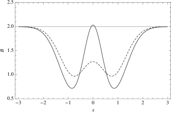
Figure 1: Function $f_{n}$ of Eq. (65) versus $x$ for $n=2$ (dashed line) and $n=3$ (solid line).

IV.3 Photon-Number tomography

Considering the state (57) its number tomogram (15) can be computed as

$$p(m_{1},\ldots m_{n},\alpha_{1},\ldots\alpha_{n}) =\prod_{i=1}^{n}\frac{|\alpha_{i}|^{2m_{i}-2}}{m_{i}!}e^{-|\alpha_{i}|^{2}}\left|\prod_{i=1}^{n}\alpha_{i}+\prod_{i=1}^{n}(m_{i}-|\alpha_{i}|^{2})\right|^{2}.$$ (66)

We further choose the sets of Definition 3 as $Z_{1}=\ldots=Z_{n}=\{0\}$, $Y_{1}=\ldots=Y_{n}=\{1,2,3,\ldots\}$.

The corresponding correlation function (25) for $n=2$ is

$$E(\alpha_{1},\alpha_{2})=e^{-|\alpha_{1}|^{2}-|\alpha_{2}|^{2}} \left[2+4\Re(\alpha_{1}\alpha_{2})+2|\alpha_{1}|^{2}|\alpha_{2}|^{2}\right.$$ (67)

$$\left.-\left(1+|\alpha_{2}|^{2}\right)e^{|\alpha_{1}|^{2}}-\left(1+|\alpha_{1}|^{2}\right)e^{|\alpha_{2}|^{2}}+e^{|\alpha_{1}|^{2}+|\alpha_{2}|^{2}}\right].$$

Furthermore, the Bell inequality for the number tomogram with $n=2$ is from (55)

$$\Bigl{|}E(\alpha^{(1)}_{1}, \alpha^{(1)}_{2})+E(\alpha^{(1)}_{1},\alpha^{(2)}_{2})+E(\alpha^{(2)}_{1},\alpha^{(1)}_{2})-E(\alpha^{(2)}_{1},\alpha^{(2)}_{2})\Bigr{|}\leqslant 2,$$ (68)

for all $\alpha^{(j)}_{1},\alpha^{(j)}_{2}\in\mathbb{C}$, $j=1,2$. Figure 2 illustrates that this inequality can be violated using (67).

Analogously, from (66) it follows that the correlation function (25) for $n=3$ is

$$E(\alpha_{1},\alpha_{2},\alpha_{3})=e^{-|\alpha_{1}|^{2}-|\alpha_{2}|^{2}-|\alpha_{3}|^{2}} \left[-4+8\Re(\alpha_{1}\alpha_{2}\alpha_{3})-4|\alpha_{1}|^{2}|\alpha_{2}|^{2}|\alpha_{3}|^{2}\right.$$ (69)

$$\left.+2\left(e^{|\alpha_{1}|^{2}}+e^{|\alpha_{2}|^{2}}+e^{|\alpha_{3}|^{2}}\right)+2|\alpha_{2}|^{2}|\alpha_{3}|^{2}e^{|\alpha_{1}|^{2}}\right.$$

$$\left.+2|\alpha_{1}|^{2}|\alpha_{2}|^{2}e^{|\alpha_{3}|^{2}}+2|\alpha_{1}|^{2}|\alpha_{3}|^{2}e^{|\alpha_{2}|^{2}}\right.$$

$$\left.-\left(1+|\alpha_{1}|^{2}\right)e^{|\alpha_{2}|^{2}+|\alpha_{3}|^{2}}-\left(1+|\alpha_{2}|^{2}\right)e^{|\alpha_{1}|^{2}+|\alpha_{3}|^{2}}\right.$$

$$\left.-\left(1+|\alpha_{3}|^{2}\right)e^{|\alpha_{1}|^{2}+|\alpha_{2}|^{2}}+e^{|\alpha_{1}|^{2}+|\alpha_{2}|^{2}+|\alpha_{3}|^{2}}\right].$$

This time the Bell inequality for the number tomogram reads from (52)

$$\Bigl{|}E(\alpha^{(1)}_{1},\alpha^{(1)}_{2},\alpha^{(2)}_{3})+E(\alpha^{(1)}_{1},\alpha^{(2)}_{2},\alpha^{(1)}_{2})+E(\alpha^{(2)}_{1},\alpha^{(1)}_{2},\alpha^{(1)}_{2})-E(\alpha^{(2)}_{1},\alpha^{(2)}_{2},\alpha^{(2)}_{2})\Bigr{|}\leqslant 2.$$ (70)

This inequality, by numerical checking, results never violated with (69) and an example of the behavior of the l.h.s. is shown in figure 2.

By also choosing $Z_{1}=\ldots=Z_{n}=\{0,\ldots,m\}$, $Y_{1}=\ldots=Y_{n}=\{m+1,m+2,\ldots\}$, with $m>0$, neither (68) nor (70) will result (by numerical checking) ever violated by using (67) and (69) respectively.

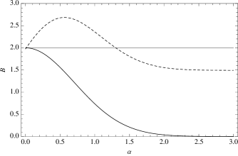
Figure 2: The left hand side of (68) as a function of $\alpha^{(2)}_{2}$ (dashed line); the other parameters are given by $\alpha^{(1)}_{1}=0.165$, $\alpha^{(1)}_{2}=-0.165$, $\alpha^{(2)}_{1}=-0.559$. The left hand side of (70) as a function of $\alpha^{(2)}_{2}$ (dashed line); the other parameters are given by $\alpha^{(1)}_{1}=\alpha^{(1)}_{2}=0$, $\alpha^{(1)}_{3}=5.936$, $\alpha^{(2)}_{1}4.767$, $\alpha^{(2)}_{3}=4$.

V Concluding remarks

As we have seen from the previous examples the use of finite (namely $2^{n}$) number of tomograms within a tomographic realization may lead to the evidence of nonlocality. Actually, it results that finite dimensional systems by means of spin tomograms allow for the best evidence of nonlocality. In contrast, violations of Bell inequalities seem much harder to uncover in infinite dimensional systems where ${\cal H}=L_{2}(\mathbb{R})$. Given that we have considered in both cases the same (entangled) state (57), this difference, according to Ref. SAM , must be ascribed to the diversity of observables employed (from which the tomograms stem). However, we argue that also the way the spectrum of an observable is binned could play a role. As matter of fact the choices made in Sections IV.2 and IV.3 for $Y_{k}$ and $Z_{k}$ do not exhaust all possibilities of these measurable sets. Unfortunately looking at Bell inequalities violations using optical tomograms (resp. photon number tomograms) by scanning the possible sets $Y_{k}$ and $Z_{k}$ appears a daunting task.

All in all the advantage of the tomographic approach is to allow to to find the large violations of Bell inequalities typical of spin systems also in infinite dimensional systems. In fact, introducing in $L_{2}(\mathbb{R})^{\otimes n}$ the following local pseudo-spin operators MISTA

$$\hat{S}^{(k)}_{x} = \sum\limits^{+\infty}_{n_{k}=0}\Bigl{(}|2n_{k}\rangle\langle 2n_{k}+1|+|2n_{k}+1\rangle\langle 2n_{k}|\Bigr{)},$$

$$\ \hat{S}^{(k)}_{y} = -i\sum\limits^{+\infty}_{n_{k}=0}\Bigl{(}|2n_{k}\rangle\langle 2n_{k}+1|-|2n_{k}+1\rangle\langle 2n_{k}|\Bigr{)},$$

$$\ \hat{S}^{(k)}_{z} = \sum\limits^{+\infty}_{n_{k}=0}(-1)^{n_{k}}|n_{k}\rangle\langle n_{k}|,$$

where $|n_{k}\rangle$ are Fock states of the $k$th subsystem, we can derive the tomograms of the spin tomography realized with the above operators from those of any other tomographic scheme (see e.g. QSO97 ). The price one ought to pay in such a case is the completeness of the set of starting tomograms, (i.e. a number of tomograms much greater than $2^{n}$).

Appendix A

Lemma 1

For any coefficients $a_{\boldsymbol{j}}=a_{j_{1},\ldots,j_{n}}$ ($\boldsymbol{j}=(j_{1},\ldots,j_{n})$) of (47) and for any angles $\theta^{(1)}_{k}$, $\theta^{(2)}_{k}$ ($k=1,\ldots,n$) we have

$$\frac{1}{2^{n}}\left|\sum^{2}_{\boldsymbol{j}=1}a_{\boldsymbol{j}}\cos\left(\theta^{(j_{1})}_{1}+\ldots+\theta^{(j_{n})}_{n}\right)\right|\leqslant 2^{(n-1)/2}.$$ (71)

The equality is attained with coefficients from (52), (55).

Proof. To estimate the l.h.s. of (71) note that

$$\left|\sum^{2}_{\boldsymbol{j}=1}a_{\boldsymbol{j}}\cos\left(\theta^{(j_{1})}_{1}+\ldots+\theta^{(j_{n})}_{n}\right)\right|\leqslant\left|\sum^{2}_{\boldsymbol{j}=1}a_{\boldsymbol{j}}e^{i\left(\theta^{(j_{1})}_{1}+\ldots+\theta^{(j_{n})}_{n}\right)}\right|,$$ (72)

so we need to estimate the last sum. To this end we use (47) obtaining

$$\left|\sum^{2}_{\boldsymbol{j}=1}a_{\boldsymbol{j}}e^{i\left(\theta^{(j_{1})}_{1}+\ldots+\theta^{(j_{n})}_{n}\right)}\right|=\sum_{\varepsilon_{1},\ldots,\varepsilon_{n}=\pm 1}c(\varepsilon_{1},\ldots,\varepsilon_{n})\prod^{n}_{k=1}\Bigl{(}e^{i\theta^{(1)}_{k}}+\varepsilon_{k}e^{i\theta^{(2)}_{k}}\Bigr{)}.$$ (73)

Next we define

$$\theta_{k}=\frac{\theta^{(1)}_{k}-\theta^{(2)}_{k}}{2},\quad\varphi_{k}=\frac{\theta^{(1)}_{k}+\theta^{(2)}_{k}}{2}.$$ (74)

so that the r.h.s. of (73) simplifies to

$$2^{n}e^{i(\varphi_{1}+\ldots+\varphi_{n})}\sum_{\varepsilon_{1},\ldots,\varepsilon_{n}=\pm 1}c(\varepsilon_{1},\ldots,\varepsilon_{n})\prod^{n}_{k=1}a_{k}(\varepsilon_{k}),$$

where $a_{k}(+1)=\cos\theta_{k}$ and $a_{k}(-1)=i\sin\theta_{k}$. Taking into account that we use absolute value in (72) and divide by $2^{n}$ in (71) we have to prove the following inequality

$$\left|\sum_{\varepsilon_{1},\ldots,\varepsilon_{n}=\pm 1}c(\varepsilon_{1},\ldots,\varepsilon_{n})\prod^{n}_{k=1}a_{k}(\varepsilon_{k})\right|\leqslant 2^{(n-1)/2},$$ (75)

for any $\pm 1$-valued function $c(\varepsilon_{1},\ldots,\varepsilon_{n})$. We employ the induction method. For $n=1$ we simply have

$$\Bigl{|}c(+1)\cos\theta_{1}+c(-1)i\sin\theta_{1}\Bigr{|}=1=2^{(1-1)/2}.$$

Then, we can write the sum in (75) as

$$\sum_{\varepsilon_{1},\ldots,\varepsilon_{n}=\pm 1}c(\varepsilon_{1},\ldots,\varepsilon_{n})\prod^{n}_{k=1}a_{k}(\varepsilon_{k}) \equiv A_{n-1}\cos\theta_{n}+iB_{n-1}\sin\theta_{n},$$

$$= \sum\limits_{\varepsilon_{1},\ldots,\varepsilon_{n-1}=\pm 1}c(\varepsilon_{1},\ldots,\varepsilon_{n-1},+1)\prod^{n-1}_{k=1}a_{k}(\varepsilon_{k})\cos\theta_{n}$$

$$+i\sum\limits_{\varepsilon_{1},\ldots,\varepsilon_{n-1}=\pm 1}c(\varepsilon_{1},\ldots,\varepsilon_{n-1},-1)\prod^{n-1}_{k=1}a_{k}(\varepsilon_{k})\sin\theta_{n}$$

where, according to the induction assumption, we have

$$|A_{n-1}|,\;|B_{n-1}|\leqslant 2^{(n-2)/2}.$$ (76)

The sum in (75) can be estimated in the following way

$$\left|\sum_{\varepsilon_{1},\ldots,\varepsilon_{n}=\pm 1}c(\varepsilon_{1},\ldots,\varepsilon_{n})\prod^{n}_{k=1}a_{k}(\varepsilon_{k})\right| = \Bigl{|}A_{n-1}\cos\theta_{n}+iB_{n-1}\sin\theta_{n}\Bigr{|}$$

$$\leqslant \sqrt{|A_{n-1}|^{2}+|B_{n-1}|^{2}}\leqslant 2^{(n-1)/2}.$$

Now we show that with the coefficients of (52) or (55) the maximal value $2^{(n-1)/2}$ is attained. Due to (72) we need to estimate the sum

$$S_{n}=\frac{1}{2^{n+(n-1)/2}}\sum^{2}_{j_{1},\ldots,j_{n}=1}a_{j_{1},\ldots,j_{n}}e^{i\left(\theta^{(j_{1})}_{1}+\ldots+\theta^{(j_{n})}_{n}\right)}$$ (77)

and show that it can be equal to one by absolute value. First, let us consider the case of an odd $n$. From (55) we have

$$a_{j_{1},\ldots,j_{n}}=2^{(n+1)/2}(-1)^{\delta(j_{1},\ldots,j_{n})},\quad\quad(j_{1},\ldots,j_{n})\in J.$$

Furthermore, from (50) it is

$$S_{n}=\frac{1}{2^{n}i}\left[\prod^{n}_{k=1}\left(e^{i\theta^{(1)}}_{k}+ie^{i\theta^{(2)}}_{k}\right)-\prod^{n}_{k=1}\left(e^{i\theta^{(1)}}_{k}-ie^{i\theta^{(2)}}_{k}\right)\right].$$

Taking into account that each term in these products can be written as

$$e^{i\theta^{(1)}}_{k}\pm e^{i\tilde{\theta}^{(2)}}_{k},\quad\tilde{\theta}^{(2)}_{k}=\theta^{(2)}_{k}+\pi/2,$$

and using the relations (74), $S_{n}$ can be simplified to

$$S_{n}=\frac{1}{i}\left(\prod^{n}_{k=1}\cos\theta^{\prime}_{k}\pm i\prod^{n}_{k=1}\sin\theta^{\prime}_{k}\right)\,e^{i(\varphi^{\prime}_{1}+\ldots+\varphi^{\prime}_{n})},$$

where $\theta^{\prime}_{k}=\theta_{k}-\pi/4$, $\varphi^{\prime}_{k}=\varphi_{k}+\pi/4$. It is clear that the imaginary part of the sum $S_{n}$ takes its maximal absolute value $1$ when, for example, $\theta_{k}=\varphi_{k}=0$ for $k=1,\ldots,n$.

Now we consider the case of an even $n$. The coefficients $a_{j_{1},\ldots,j_{n}}$ in this case come from (52)

$$a_{j_{1},\ldots,j_{n}}=2^{n/2}(-1)^{\tilde{\delta}(j_{1},\ldots,j_{n})},$$

and the sum $S_{n}$ (77) becomes

$$S_{n} =\frac{1}{i2^{n}\sqrt{2}}(e^{i\theta^{(1)}}_{n}+e^{i\theta^{(2)}}_{n})\left[\prod^{n-1}_{k=1}\left(e^{i\theta^{(1)}}_{k}+e^{i\tilde{\theta}^{(2)}}_{k}\right)-\prod^{n-1}_{k=1}\left(e^{i\theta^{(1)}}_{k}-e^{i\tilde{\theta}^{(2)}}_{k}\right)\right]$$

$$+\frac{1}{i2^{n}\sqrt{2}}(e^{i\theta^{(1)}}_{n}e^{i\theta^{(2)}}_{n})\left[\prod^{n-1}_{k=1}\left(e^{i\tilde{\theta}^{(1)}}_{k}+e^{i\theta^{(2)}}_{k}\right)-\prod^{n-1}_{k=1}\left(e^{i\tilde{\theta}^{(1)}}_{k}-e^{i\theta^{(2)}}_{k}\right)\right].$$

According to (74) $S_{n}$ can be simplified to

$$S_{n} =\frac{e^{i\varphi}}{\sqrt{2}}\left[\left(i\prod^{n-1}_{k=1}\cos\theta^{\prime}_{k}\mp\prod^{n-1}_{k=1}\sin\theta^{\prime}_{k}\right)\cos\theta_{n}+\left(\prod^{n-1}_{k=1}\cos\theta^{\prime\prime}_{k}\pm i\prod^{n-1}_{k=1}\sin\theta^{\prime\prime}_{k}\right)\sin\theta_{n}\right],$$

where $\theta^{\prime}_{k}=\theta_{k}-\pi/4$, $\theta^{\prime\prime}_{k}=\theta_{k}+\pi/4$ and $\varphi=\varphi_{1}+\ldots\varphi_{n}+(n-1)\pi/4$. The imaginary part of $S_{n}$ is (when $\varphi=0$)

$$|\mathrm{Im}(S_{n})| =\frac{1}{\sqrt{2}}\left|\cos\theta_{n}\prod^{n-1}_{k=1}\cos(\theta_{k}-\pi/4)\pm\sin\theta_{n}\prod^{n-1}_{k=1}\sin(\theta_{k}+\pi/4)\right|.$$

It is clear that this expression takes its maximal value $1$ when $\theta_{k}=\pi/4$, $k=1,\ldots,n-1$, and $\theta_{n}=\pm\pi/4$. This completes the proof.   

References