Mechanics-based solution verification for porous media models
   
An e-print of the paper is available on arXiv: 1501.02581.

Authored by

M. Shabouei

Graduate Student, University of Houston.

K. B. Nakshatrala

Department of Civil & Environmental Engineering
University of Houston, Houston, Texas 77204–4003.
phone: +1-713-743-4418, e-mail: knakshatrala@uh.edu
website: http://www.cive.uh.edu/faculty/nakshatrala

Abstract.

This paper presents a new approach to verify accuracy of computational simulations. We develop mathematical theorems which can serve as robust a posteriori error estimation techniques to identify numerical pollution, check the performance of adaptive meshes, and verify numerical solutions. We demonstrate performance of this methodology on problems from flow thorough porous media. However, one can extend it to other models. We construct mathematical properties such that the solutions to Darcy and Darcy-Brinkman equations satisfy them. The mathematical properties include the total minimum mechanical power, minimum dissipation theorem, reciprocal relation, and maximum principle for the vorticity. All the developed theorems have firm mechanical bases and are independent of numerical methods. So, these can be utilized for solution verification of finite element, finite volume, finite difference, lattice Boltzmann methods and so forth. In particular, we show that, for a given set of boundary conditions, Darcy velocity has the minimum total mechanical power of all the kinematically admissible vector fields. We also show that a similar result holds for Darcy-Brinkman velocity. We then show for a conservative body force, the Darcy and Darcy-Brinkman velocities have the minimum total dissipation among their respective kinematically admissible vector fields. Using numerical examples, we show that the minimum dissipation and total mechanical power theorems can be utilized to identify pollution errors in numerical solutions. The solutions to Darcy and Darcy-Brinkman equations are shown to satisfy a reciprocal relation, which has the potential to identify errors in the numerical implementation of boundary conditions. It is also shown that the vorticity under both steady and transient Darcy-Brinkman equations satisfy maximum principles if the body force is conservative and the permeability is homogeneous and isotropic. A discussion on the nature of vorticity under steady and transient Darcy equations is also presented. Using several numerical examples, we will demonstrate the predictive capabilities of the proposed a posteriori techniques in assessing the accuracy of numerical solutions for a general class of problems, which could involve complex domains and general computational grids.

1. INTRODUCTION

1.1. Validation and verification (V&V)

Errors can arise in both physical modeling and numerical simulation. The study of errors due to physical modeling is referred to as validation, and the study of error in a numerical simulation is referred to as verification. As Blottner [Blottner, 1990] nicely puts it, validation is to solve “right governing equations” and verification is to solve “governing equation right”. Validation errors arise when a model is used out of its application range. The errors in the verification, on the other hand, can arise from three broad sources including numerical errors, round-off errors (due to the finite precision arithmetic), and programming mistakes [Oberkampf et al., 2004]. Basically, the verification is to ensure that the code produces a solution with some degree of accuracy, and the numerical solution is consistent. Verification itself is conducted into two modes: verification of code and verification of calculation [Roache, 1998; Rider et al., 2016]. Verification of code addresses the question of whether the numerical algorithms have been programmed and implemented correctly in the code. The two currently popular approaches to verify a code are the method of exact solutions (MES) and the method of manufactured solutions (MMS). More thorough discussions on MES and MMS can be found in [Knupp and Salari, 2003; Roy et al., 2004; Roache, 1998].

Verification of calculation (which is also referred to as solution verification) estimates the overall magnitude (not just the order) of the numerical errors in a calculation, and the procedure invariably involves a posteriori error estimation [Salari and Knupp, 2000]. The numerical errors in the solution verification can arise from two different sources including discretization errors and solution errors. The discretization errors refer to all the errors caused by conversion of the governing equations (PDEs and boundary conditions) into discrete algebraic equations whereas the solution errors refer to the errors in approximate solution of the discrete equations. The numerical errors may arise from insufficient mesh resolution, improper selection of time-step, and incomplete iterative convergence. For more details on verification of calculation, see [Roy et al., 2004; Salari and Knupp, 2000; Roache, 1997, 1998; Babuška and Oden, 2004; Oberkampf and Blottner, 1998; Oberkampf et al., 2004; Rider et al., 2016].

1.2. A posteriori techniques

The aim of a posteriori error estimation is to assess the accuracy of the numerical approximation in the terms of known quantities such as geometrical properties of computational grid, the input data, and the numerical solution. A posteriori error techniques monitor various forms of the error in the numerical solution such as velocity, stress, mean fluxes, and drag and lift coefficients [Becker and Rannacher, 2001]. Such error estimation differ from a priori error estimates in that the error controlling parameters depend on unknown quantities. A priori error estimation investigates the stability and convergence of a solver and can give rough information on the asymptotic behavior of errors in calculations when grid parameters are changed appropriately [Ainsworth and Oden, 1997].

Moreover, discontinuities and singularities commonly occur in fluid dynamics, solid mechanics, and structural dynamics and it is a subject of intense research and grave concern in error estimation [Oberkampf et al., 2004]. Some representative works on pollution errors due to singularities and discontinuities are [Babuška and Oh, 1987; Babuška et al., 1995, 1997; Oden et al., 1998; Roache, 1998; Botella and Peyret, 2001].

The question that still remains is how to verify the accuracy of numerical solutions, especially for realistic problems. Below are some specific challenges that a computational scientist may face in using numerical simulators:

1. How much mesh refinement is required to obtain solutions with desired degree of accuracy for a problem that does not have an analytical or reference solution?

2. Will the chosen mesh be able to resolve singularities in the solution and avoid pollution errors? That is, can we identify whether a particular type of mesh suffers from pollution errors for a problem with singularities?

3. Has the computer implementation been done properly?

4. Is the chosen numerical formulation accurate/appropriate for the chosen problem?

In the literature, one finds the usual approach of employing tools from functional analysis to obtain a priori estimates and assess stability. For example, see [Brezzi and Fortin, 1991; Babuška and Strouboulis, 2001]. On the other hand, this paper aims to address the aforementioned challenges by providing various a posteriori techniques with firm mechanics underpinning.

In the current study, we develop new methodology to verify the accuracy and convergence of numerical solutions. In addition, the presented a posteriori error estimation approach is able to identify pollution in computational domains and check whether adaptive grids can resolve the numerical pollution. The proposed criteria is independent of employed numerical method. It means, our technique is able to verify the solution of all numerical methods including finite element, finite volume, finite difference and lattice Boltzmann. Hence, we named it mechanics-based solution verification. Then, we show performance of this powerful tool on problems from flow thorough porous solid. But, it is not restricted to porous media models and it is extendable to other problems.

1.3. Popular porous media models

The simplest and yet the most popular model that describes the flow of an incompressible fluid in a rigid porous media is the Darcy model [Darcy, 1856]. The Darcy equations posed several challenges to the computational community but played a crucial role in the development of mixed and stabilized formulations in finite element method (FEM) [Masud and Hughes, 2002; Nakshatrala et al., 2006]. Brinkman [Brinkman, 1947a, b] proposed an extension to the Darcy model which is commonly referred to as the Darcy-Brinkman model. In addition to drag between the fluid and porous solid, Darcy-Brinkman model accounts for viscous term (friction between fluid layers). It is, however, not possible to obtain analytical solutions under these models, and one commonly seeks numerical solutions for realistic problems.

Since the aim of this paper is a posteriori error estimation, we assume that the code has already been verified for the Darcy and Darcy-Brinkman class of problems so that programming mistakes are not an issue. Likewise, we are not also concerned with validation. It means that the Darcy and Darcy-Brinkman models are physically adequate to model the problems. Moreover, the solution verification requires confirmation of grid convergence which is one of the most common and reliable error estimation methods [Roache, 1997]. Similar to grid convergence studies, we address only solution verification.

1.4. Organization of the paper

Section 2 presents the governing equations arising from the Darcy and Darcy-Brinkman models. In Section 3, we propose various mathematical properties that the solutions to these governing equations satisfy. We also discuss how these properties can be utilized as robust a posteriori criteria to assess the accuracy of numerical solutions. Section 4 presents several steady-state numerical results to illustrate the predictive capabilities of the proposed a posteriori criteria with respect to singularities, pollution errors, and discretization errors in the implementation of (Neumann) boundary conditions. In Section 5, we utilize synthetic reservoir data to demonstrate the usefulness of the proposed a posteriori techniques, especially for problems involving spatially heterogeneous permeability properties. Section 6 discusses a posteriori criteria for transient problems, and presents representative numerical results in support of the theoretical predictions. Finally, conclusions are drawn in Section 7.

2. DARCY AND DARCY-BRINKMAN MODELS

Let $\Omega\subset\mathbb{R}^{nd}$ be an open and bounded domain, where “$nd$” denotes the number of spatial dimensions. We shall denote the set closure of $\Omega$ by $\overline{\Omega}$. Let $\partial\Omega:=\overline{\Omega}-\Omega$ denote the boundary, which is assumed to be piecewise smooth. A spatial point in $\overline{\Omega}$ is denoted by $\mathbf{x}$. The spatial gradient and divergence operators are, respectively, denoted as $\mathrm{grad}[\cdot]$ and $\mathrm{div}[\cdot]$. Let $\mathbf{v}:~{}\Omega\rightarrow\mathbb{R}^{nd}$ denote the velocity field and $p:\Omega\rightarrow\mathbb{R}$ denote the pressure field. The symmetric part of the gradient of velocity is denoted by $\mathbf{D}(\mathbf{x})$. That is,

$$\mathbf{D}(\mathbf{x})=\frac{1}{2}\left(\mathrm{grad}[\mathbf{v}]+\mathrm{grad}[\mathbf{v}]^{\mathrm{T}}\right)$$ (2.1)

The unit outward normal to the boundary is denoted as $\widehat{\mathbf{n}}(\mathbf{x})$. The boundary is divided into two parts: $\Gamma^{v}$ and $\Gamma^{t}$. $\Gamma^{v}$ is the part of the boundary on which the velocity is prescribed, and $\Gamma^{t}$ is that part of the boundary on which the traction is prescribed. For mathematical well-posedness, we have $\Gamma^{v}\cap\Gamma^{t}=\emptyset$ and $\Gamma^{v}\cup\Gamma^{t}=\partial\Omega$.

The porous media models that will be considered in this paper are the Darcy and Darcy-Brinkman models. Both these models describe the flow of an incompressible fluid through rigid porous media. We completely neglect the motion of the porous solid. The Cauchy stress in the Darcy and Darcy-Brinkman models, respectively, take the following form:

$$\mathbf{T}(\mathbf{x})=-p(\mathbf{x})\mathbf{I}$$ (2.2a)

$$\mathbf{T}(\mathbf{x})=-p(\mathbf{x})\mathbf{I}+2\mu\mathbf{D}(\mathbf{x})$$ (2.2b)

where $\mathbf{I}$ denotes the second-order identity tensor, and $\mu$ is the dynamic coefficient of viscosity. The steady-state governing equations based on the Darcy model can be written as follows:

$$\alpha(\mathbf{x})\mathbf{v}(\mathbf{x})+\mathrm{grad}[p(\mathbf{x})]=\rho\mathbf{b}(\mathbf{x})\quad \mbox{in}\;\Omega$$ (2.3a)

$$\mathrm{div}[\mathbf{v}(\mathbf{x})]=0\quad \mbox{in}\;\Omega$$ (2.3b)

$$\mathbf{v}(\mathbf{x})\cdot\widehat{\mathbf{n}}(\mathbf{x})=v_{n}(\mathbf{x})\quad \mbox{on}\;\Gamma^{v}$$ (2.3c)

$$p(\mathbf{x})=p_{0}(\mathbf{x})\quad \mbox{on}\;\Gamma^{t}$$ (2.3d)

where $\alpha(\mathbf{x})$ is the drag coefficient, $\rho$ is the density of the fluid, $\mathbf{b}(\mathbf{x})$ is the specific body force, $v_{n}(\mathbf{x})$ is the prescribed normal component of the velocity, and $p_{0}(\mathbf{x})$ is the prescribed pressure. The steady-state governing equations based on the Darcy-Brinkman model take the following form:

$$\alpha(\mathbf{x})\mathbf{v}(\mathbf{x})+\mathrm{grad}[p(\mathbf{x})]-\mathrm{div}\left[2\mu\mathbf{D}\right]=\rho\mathbf{b}(\mathbf{x})\quad \mbox{in}\;\Omega$$ (2.4a)

$$\mathrm{div}[\mathbf{v}(\mathbf{x})]=0\quad \mbox{in}\;\Omega$$ (2.4b)

$$\mathbf{v}(\mathbf{x})=\mathbf{v}^{\mathrm{p}}(\mathbf{x})\quad \mbox{on}\;\Gamma^{v}$$ (2.4c)

$$\mathbf{T}\mathbf{\widehat{n}}(\mathbf{x})=\mathbf{t}^{\mathrm{p}}(\mathbf{x})\quad \mbox{on}\;\Gamma^{t}$$ (2.4d)

where $\mathbf{v}^{\mathrm{p}}(\mathbf{x})$ is the prescribed velocity vector, and $\mathbf{t}^{\mathrm{p}}(\mathbf{x})$ is the prescribed traction. We shall call a vector-field to be Darcy velocity if satisfies equations (2.3a)–(2.3d). We shall call a vector field to be Darcy-Brinkman velocity if it satisfies equations (2.4a)–(2.4d).

Equations (2.3a) and (2.4a) can be obtained from the balance of linear momentum under the mathematical framework offered by the theory of interacting continua [Nakshatrala and Rajagopal, 2011]. The drag term $\alpha(\mathbf{x})\mathbf{v}(\mathbf{x})$ models the frictional force between the fluid and the porous solid. The term $\mathrm{div}[2\mu\mathbf{D}]$ in the Darcy-Brinkman model arises due to the internal friction between the layers of the fluid. The pressure $p(\mathbf{x})$ is an undetermined multiplier that arises due to the enforcement of the incompressibility constraint given by equations (2.3b) and (2.4b). The drag coefficient is related to the coefficient of viscosity of the fluid and the permeability $k(\mathbf{x})$ as follows:

$$\alpha(\mathbf{x})=\frac{\mu}{k(\mathbf{x})}$$ (2.5)

In general, it is not possible to obtain analytical solutions to the systems of equations given by either (2.3a)–(2.3d) or (2.4a)–(2.4d). Hence, one needs to resort to numerical solutions. This paper does not concern with developing new numerical formulations to solve the aforementioned mathematical models. The paper instead focuses on deriving mathematical properties with firm mechanics underpinning that the solutions to these mathematical models satisfy. We shall then illustrate how these mathematical properties can serve as robust “a posteriori” criteria to assess the accuracy of numerical solutions.

3. MATHEMATICAL PROPERTIES: STATEMENTS AND DERIVATIONS

In the remainder of this paper, we shall refer to a vector field $\widetilde{\mathbf{v}}:~{}\Omega\rightarrow\mathbb{R}^{nd}$ as kinematically admissible if it satisfies the following conditions:

1. $\widetilde{\mathbf{v}}(\mathbf{x})$ is solenoidal (i.e., $\mathrm{div}[\widetilde{\mathbf{v}}(\mathbf{x})]=0\;\mathrm{in}\;\Omega$), and

2. $\widetilde{\mathbf{v}}(\mathbf{x})$ satisfies the boundary conditions.

It needs to emphasized that a kinematically admissible vector field need not satisfy the balance of linear momentum given by equation (2.3a) or (2.4a). Clearly, the Darcy velocity and the Darcy-Brinkman velocity are kinematically admissible vector fields. For some of the results presented in this paper, we will need the body force to be conservative, which is a common terminology in potential theory [Kellogg, 2010]. The body force $\rho\mathbf{b}(\mathbf{x})$ is said to be conservative if there exists a scalar potential $\psi(\mathbf{x})$ such that $\rho\mathbf{b}(\mathbf{x})=-\mathrm{grad}[\psi]$. We shall define the dissipation functional as follows:

$$\Phi[\mathbf{v}]:=\left\{\begin{array}[]{ll}\int_{\Omega}\alpha(\mathbf{x})\mathbf{v}(\mathbf{x})\cdot\mathbf{v}(\mathbf{x})\;\mathrm{d}\Omega&\mbox{Darcy model}\\ \int_{\Omega}\alpha(\mathbf{x})\mathbf{v}(\mathbf{x})\cdot\mathbf{v}(\mathbf{x})\;\mathrm{d}\Omega+\int_{\Omega}2\mu\mathbf{D}(\mathbf{x})\cdot\mathbf{D}(\mathbf{x})\;\mathrm{d}\Omega&\mbox{Darcy-Brinkman model}\end{array}\right.$$ (3.3)

Since $\alpha>0$ and $\mu>0$, it is straightforward to check that $\Phi[\mathbf{v}]$ is a norm. In fact, it can be shown that $\Phi[\mathbf{v}]$ under the Darcy model is equivalent to the natural norm in $(L^{2}({\Omega}))^{nd}$, where $(L^{2}(\Omega))^{nd}$ is a space of square integrable vector fields defined from $\Omega$ to $\mathbb{R}^{nd}$. Similarly, it can be shown that $\Phi[\mathbf{v}]$ under the Darcy-Brinkman model is equivalent to the natural norm in $(H^{1}(\Omega))^{nd}$, which is a Sobolev space. For further details on function spaces and norms, refer to [Evans, 1998].

In this section, we shall present four important mathematical properties that the solutions to Darcy equations and Darcy-Brinkman equations satisfy. These properties will be referred to as (i) the minimum total mechanical power theorem, (ii) the minimum dissipation theorem, (iii) reciprocal relation, and (iv) maximum principle for vorticity. As a passing comment, we will employ the minimum dissipation theorem to show the uniqueness of solution for Darcy equations and Darcy-Brinkman equations. In the porous media literature, these results have neither been discussed nor utilized to solve problems. More importantly, these results have not been used to assess the accuracy and convergence of numerical solutions of porous media models. For example, it will be shown that the minimum total mechanical power theorem can be utilized to assess the accuracy of the implementation of both Dirichlet and Neumann boundary conditions. On the other hand, the minimum dissipation theorem can be utilized to identify pollution errors in the numerical solution. Herein, we give detailed mathematical proofs for Darcy-Brinkman equations. We however provide comments on the corresponding proofs for Darcy equations.

Theorem 1 (Minimum total mechanical power theorem).

Let $\mathbf{v}(\mathbf{x})$ be the Darcy-Brinkman velocity vector field. Then, any kinematically admissible vector field $\widetilde{\mathbf{v}}(\mathbf{x})$ satisfies the following inequality:

$$\varepsilon_{\mathrm{TMP}}[\mathbf{v}]\leq\varepsilon_{\mathrm{TMP}}[\widetilde{\mathbf{v}}]$$ (3.4)

where

$$\varepsilon_{\mathrm{TMP}}[\mathbf{z}]:=\frac{1}{2}\Phi[\mathbf{z}]-\int_{\Omega}\rho\mathbf{b}(\mathbf{x})\cdot\mathbf{z}(\mathbf{x})\;\mathrm{d}\Omega-\int_{\Gamma^{t}}\mathbf{t}^{\mathrm{p}}(\mathbf{x})\cdot\mathbf{z}(\mathbf{x})\;\mathrm{d}\Gamma$$ (3.5)

That is, for given boundary conditions, body force and tractions; the Darcy-Brinkman velocity will have the minimum total mechanical power among all the possible kinematically admissible vector fields.

Proof.

Let

$$\delta\mathbf{v}(\mathbf{x}):=\widetilde{\mathbf{v}}(\mathbf{x})-\mathbf{v}(\mathbf{x})$$ (3.6a)

$$\delta\mathbf{D}(\mathbf{x}):=\widetilde{\mathbf{D}}(\mathbf{x})-\mathbf{D}(\mathbf{x})$$ (3.6b)

From the hypothesis of the theorem, $\delta\mathbf{v}(\mathbf{x})$ satisfies the following relations:

$$\delta\mathbf{v}(\mathbf{x})=\mathbf{0}\quad\forall\mathbf{x}\in\partial\Omega$$ (3.7a)

$$\mathrm{div}[\delta\mathbf{v}]=0\quad\forall\mathbf{x}\in\Omega$$ (3.7b)

Let us start with the dissipation due to the vector field $\widetilde{\mathbf{v}}(\mathbf{x})$:

$$\Phi[\widetilde{\mathbf{v}}(\mathbf{x})] :=\int_{\Omega}\alpha(\mathbf{x})\widetilde{\mathbf{v}}(\mathbf{x})\cdot\widetilde{\mathbf{v}}(\mathbf{x})\;\mathrm{d}\Omega+\int_{\Omega}2\mu\widetilde{\mathbf{D}}(\mathbf{x})\cdot\widetilde{\mathbf{D}}(\mathbf{x})\;\mathrm{d}\Omega$$

$$=\int_{\Omega}\alpha(\mathbf{x})\left(\delta\mathbf{v}(\mathbf{x})+\mathbf{v}(\mathbf{x})\right)\cdot\left(\delta\mathbf{v}(\mathbf{x})+\mathbf{v}(\mathbf{x})\right)\;\mathrm{d}\Omega+\int_{\Omega}2\mu\left(\delta\mathbf{D}(\mathbf{x})+\mathbf{D}(\mathbf{x})\right)\cdot\left(\delta\mathbf{D}(\mathbf{x})+\mathbf{D}\mathbf{x})\right)\;\mathrm{d}\Omega$$

$$\geq 2\int_{\Omega}\alpha(\mathbf{x})\delta\mathbf{v}(\mathbf{x})\cdot\mathbf{v}(\mathbf{x})\;\mathrm{d}\Omega+2\int_{\Omega}2\mu\delta\mathbf{D}(\mathbf{x})\cdot\mathbf{D}(\mathbf{x})\;\mathrm{d}\Omega+\Phi{[\mathbf{v}(\mathbf{x})]}$$ (3.8)

Using equations (2.4a) and (2.2b) the first integral in the above equation can be written as follows:

$$\int_{\Omega}\alpha(\mathbf{x})\delta\mathbf{v}(\mathbf{x})\cdot\mathbf{v}(\mathbf{x})\;\mathrm{d}\Omega=\int_{\Omega}\delta\mathbf{v}(\mathbf{x})\cdot\left(\rho\mathbf{b}(\mathbf{x})+\mathrm{div}\left[\mathbf{T}(\mathbf{x})\right]\right)\;\mathrm{d}\Omega$$ (3.9)

The symmetry of $\mathbf{D}(\mathbf{x})$ allows the second integral to be written as follows:

$$\int_{\Omega}2\mu\delta\mathbf{D}(\mathbf{x})\cdot\mathbf{D}(\mathbf{x})\;\mathrm{d}\Omega =\int_{\Omega}2\mu\;\mathrm{grad}[\delta\mathbf{v}(\mathbf{x})]\cdot\mathbf{D}(\mathbf{x})\;\mathrm{d}\Omega$$

$$=\int_{\Omega}\;\mathrm{grad}[\delta\mathbf{v}(\mathbf{x})]\cdot\left(\mathbf{T}(\mathbf{x})+p(\mathbf{x})\mathbf{I}\right)\;\mathrm{d}\Omega$$

$$=\int_{\Omega}\;\mathrm{grad}[\delta\mathbf{v}(\mathbf{x})]\cdot\mathbf{T}(\mathbf{x})\;\mathrm{d}\Omega+\int_{\Omega}\;\mathrm{div}[\delta\mathbf{v}(\mathbf{x})]\cdot p(\mathbf{x})\;\mathrm{d}\Omega$$

Noting that $\mathrm{div}[\delta\mathbf{v}]=0\;\mathrm{in}\;\Omega$ and by employing Green’s identity, we have the following:

$$\int_{\Omega}2\mu\delta\mathbf{D}(\mathbf{x})\cdot\mathbf{D}(\mathbf{x})\;\mathrm{d}\Omega =\int_{\Omega}\mathrm{div}[\mathbf{T}^{\mathrm{T}}(\mathbf{x})\;\delta\mathbf{v}(\mathbf{x})]\;\mathrm{d}\Omega-\int_{\Omega}\delta\mathbf{v}(\mathbf{x})\cdot\mathrm{div}[\mathbf{T}(\mathbf{x})]\;\mathrm{d}\Omega$$

$$=\int_{\Gamma^{t}}\delta\mathbf{v}(\mathbf{x})\cdot\mathbf{t}^{\mathrm{p}}(\mathbf{x})\;\mathrm{d}\Gamma-\int_{\Omega}\delta\mathbf{v}(\mathbf{x})\cdot\mathrm{div}[\mathbf{T}(\mathbf{x})]\;\mathrm{d}\Omega$$ (3.10)

From equations (3.9) and (3), inequality (3) can be written as follows:

$$\Phi[\widetilde{\mathbf{v}}(\mathbf{x})] \geq\Phi[\mathbf{v}(\mathbf{x})]+2\int_{\Omega}\delta\mathbf{v}(\mathbf{x})\cdot\rho\mathbf{b}(\mathbf{x})\;\mathrm{d}\Omega+2\int_{\Gamma^{t}}\delta\mathbf{v}(\mathbf{x})\cdot\mathbf{t}^{\mathrm{p}}(\mathbf{x})\;\mathrm{d}\Gamma$$ (3.11)

This completes the proof. ∎

Remark 1.

For Darcy equations (2.3a)–(2.3d), one can state the minimum total mechanical power theorem as follows: For given boundary conditions, and body force; the Darcy velocity, $\mathbf{v}(\mathbf{x})$, has the minimum total mechanical power among all the kinematically admissible vector fields. That is,

$$\frac{1}{2}\Phi[\mathbf{v}]-\int_{\Omega}\mathbf{v}(\mathbf{x})\cdot\rho\mathbf{b}(\mathbf{x})\;\mathrm{d}\Omega+\int_{\Gamma^{t}}p_{0}(\mathbf{x})\mathbf{v}(\mathbf{x})\cdot\widehat{\mathbf{n}}(\mathbf{x})\;\mathrm{d}\Gamma \leq\frac{1}{2}\Phi[\widetilde{\mathbf{v}}]-\int_{\Omega}\widetilde{\mathbf{v}}(\mathbf{x})\cdot\rho\mathbf{b}(\mathbf{x})\;\mathrm{d}\Omega$$

$$+\int_{\Gamma^{t}}p_{0}(\mathbf{x})\widetilde{\mathbf{v}}(\mathbf{x})\cdot\widehat{\mathbf{n}}(\mathbf{x})\;\mathrm{d}\Gamma\quad\forall\widetilde{\mathbf{v}}(\mathbf{x})$$ (3.12)

Theorem 2 (Minimum dissipation inequality).

Let $\mathbf{v}(\mathbf{x})$ be the Darcy-Brinkman velocity vector field, and let $\Gamma^{v}=\partial\Omega$. Then, any kinematically admissible vector field $\widetilde{\mathbf{v}}(\mathbf{x})$ satisfies the following inequality:

$$\Phi[\mathbf{v}]\leq\Phi[\widetilde{\mathbf{v}}]$$ (3.13)

That is, for given velocity boundary conditions and conservative body force, the Darcy-Brinkman velocity has the minimum total dissipation due to drag and internal friction of all the possible kinematically admissible vector fields.

Proof.

We shall employ the notation introduced in equation (3.6). Recall that the mechanical dissipation under the Darcy-Brinkman model is

$$\Phi[\mathbf{v}]=\int_{\Omega}\alpha\delta\mathbf{v}(\mathbf{x})\cdot\mathbf{v}(\mathbf{x})\;\mathrm{d}\Omega+\int_{\Omega}2\mu\delta\mathbf{D}(\mathbf{x})\cdot\mathbf{D}(\mathbf{x})\;\mathrm{d}\Omega$$ (3.14)

Let us start with the difference in total dissipation, and from inequality (3) we have:

$$\Phi[\widetilde{\mathbf{v}}(\mathbf{x})]-\Phi[\mathbf{v}(\mathbf{x})]\geq 2\int_{\Omega}\alpha\delta\mathbf{v}(\mathbf{x})\cdot\mathbf{v}(\mathbf{x})\;\mathrm{d}\Omega+2\int_{\Omega}2\mu\delta\mathbf{D}(\mathbf{x})\cdot\mathbf{D}(\mathbf{x})\;\mathrm{d}\Omega$$ (3.15)

Using Green’s identity, the first integral can be simplified as follows:

$$\int_{\Omega}\alpha\delta\mathbf{v}(\mathbf{x})\cdot\mathbf{v}(\mathbf{x})\;\mathrm{d}\Omega =\int_{\Omega}\delta\mathbf{v}(\mathbf{x})\cdot\mathrm{grad}[\psi(\mathbf{x})-p(\mathbf{x})]\;\mathrm{d}\Omega+\int_{\Omega}\delta\mathbf{v}(\mathbf{x})\cdot\mathrm{div}[2\mu\mathbf{D}(\mathbf{x})]\;\mathrm{d}\Omega$$

$$=\int_{\partial\Omega}\delta\mathbf{v}(\mathbf{x})\cdot\widehat{\mathbf{n}}(\mathbf{x})\left(\psi(\mathbf{x})-p(\mathbf{x})\right)\;\mathrm{d}\Gamma-\int_{\Omega}\mathrm{div}[\delta\mathbf{v}(\mathbf{x})]\left(\psi(\mathbf{x})-p(\mathbf{x})\right)\;\mathrm{d}\Omega$$

$$\quad+\int_{\Omega}\delta\mathbf{v}(\mathbf{x})\cdot\mathrm{div}[2\mu\mathbf{D}(\mathbf{x})]\;\mathrm{d}\Omega$$ (3.16)

Noting the symmetry of $\mathbf{D}(\mathbf{x})$ and using Green’s identity, the total dissipation due to internal friction can be simplified as follows:

$$\int_{\Omega}2\mu\delta\mathbf{D}(\mathbf{x})\cdot\mathbf{D}(\mathbf{x})\;\mathrm{d}\Omega =\int_{\Omega}2\mu\;\mathrm{grad}[\delta\mathbf{v}(\mathbf{x})]\cdot\mathbf{D}(\mathbf{x})\;\mathrm{d}\Omega$$

$$=\int_{\partial\Omega}2\mu\delta\mathbf{v}(\mathbf{x})\cdot\mathbf{D}(\mathbf{x})\widehat{\mathbf{n}}(\mathbf{x})\;\mathrm{d}\Gamma-\int_{\Omega}\delta\mathbf{v}(\mathbf{x})\cdot\mathrm{div}[2\mu\mathbf{D}(\mathbf{x})]\;\mathrm{d}\Omega$$ (3.17)

From equations (3.9)–(3), the total dissipation due to drag and internal friction satisfies:

$$\Phi[\widetilde{\mathbf{v}}(\mathbf{x})]-\Phi[\mathbf{v}(\mathbf{x})] \geq 2\int_{\partial\Omega}\delta\mathbf{v}(\mathbf{x})\cdot\widehat{\mathbf{n}}(\mathbf{x})\left(\psi(\mathbf{x})-p(\mathbf{x})\right)\;\mathrm{d}\Gamma-2\int_{\Omega}\mathrm{div}[\delta\mathbf{v}(\mathbf{x})]\left(\psi(\mathbf{x})-p(\mathbf{x})\right)\;\mathrm{d}\Omega$$

$$+2\int_{\partial\Omega}2\mu\delta\mathbf{v}(\mathbf{x})\cdot\mathbf{D}(\mathbf{x})\widehat{\mathbf{n}}(\mathbf{x})\;\mathrm{d}\Gamma=0$$ (3.18)

This completes the proof. ∎

The solutions to Darcy and Darcy-Brinkman equations posses reciprocal relations similar to the famous Betti’s reciprocal relation in the theory of linear elasticity [Truesdell and Noll, 2004; Sadd, 2009] and to a classical reciprocal relation in the area of creeping flows [Guazzelli and Morris, 2012]. The Betti’s reciprocal relation is often employed to solve a class of problems in linear elasticity, which otherwise may be difficult to solve. Mathematically, the Betti’s reciprocal relation is equivalent to the existence and symmetry of Green’s function. We now precisely state a reciprocal relation that the solutions of Darcy-Brinkman equations satisfy, and then provide a mathematical proof.

Theorem 3 (Reciprocal relation).

Assume that $\mathbf{v}^{\mathrm{p}}(\mathbf{x})=\mathbf{0}$ on $\Gamma^{v}$. Let $\left\{\mathbf{v}_{1}(\mathbf{x}),p_{1}(\mathbf{x})\right\}$ and $\left\{\mathbf{v}_{2}(\mathbf{x}),p_{2}(\mathbf{x})\right\}$ be the solutions of equations (2.4a)–(2.4d) for the prescribed data $\left\{\mathbf{b}_{1}(\mathbf{x}),\mathbf{t}^{\mathrm{p}}_{1}(\mathbf{x})\right\}$ and $\left\{\mathbf{b}_{2}(\mathbf{x}),\mathbf{t}^{\mathrm{p}}_{2}(\mathbf{x})\right\}$, respectively. Then, these fields satisfy the following relation:

$$\int_{\Omega}\rho\mathbf{b}_{1}(\mathbf{x})\cdot\mathbf{v}_{2}(\mathbf{x})\;\mathrm{d}\Omega+\int_{\Gamma^{t}}\mathbf{t}_{1}^{\mathrm{p}}(\mathbf{x})\cdot\mathbf{v}_{2}(\mathbf{x})\;\mathrm{d}\Gamma=\int_{\Omega}\rho\mathbf{b}_{2}(\mathbf{x})\cdot\mathbf{v}_{1}(\mathbf{x})\;\mathrm{d}\Omega+\int_{\Gamma^{t}}\mathbf{t}_{2}^{\mathrm{p}}(\mathbf{x})\cdot\mathbf{v}_{1}(\mathbf{x})\;\mathrm{d}\Gamma$$ (3.19)

Proof.

Let us start with the left side of equation (3.19). Noting that $\mathbf{v}^{\mathrm{p}}(\mathbf{x})=\mathbf{0}$ on $\Gamma^{v}$ and $\Gamma^{v}\cup\Gamma^{t}=\partial\Omega$, one can proceed as follows:

$$\int_{\Omega}\rho\mathbf{b}_{1}(\mathbf{x})\cdot\mathbf{v}_{2}(\mathbf{x})\;\mathrm{d}\Omega +\int_{\Gamma^{t}}\mathbf{t}_{1}^{\mathrm{p}}(\mathbf{x})\cdot\mathbf{v}_{2}(\mathbf{x})\;\mathrm{d}\Gamma=\int_{\Omega}\rho\mathbf{b}_{1}(\mathbf{x})\cdot\mathbf{v}_{2}(\mathbf{x})\;\mathrm{d}\Omega+\int_{\Gamma^{t}}\left(\mathbf{T}_{1}\widehat{\mathbf{n}}(\mathbf{x})\right)\cdot\mathbf{v}_{2}(\mathbf{x})\;\mathrm{d}\Gamma$$

$$=\int_{\Omega}\rho\mathbf{b}_{1}(\mathbf{x})\cdot\mathbf{v}_{2}(\mathbf{x})\;\mathrm{d}\Omega+\int_{\partial\Omega}\left(\mathbf{T}_{1}\widehat{\mathbf{n}}(\mathbf{x})\right)\cdot\mathbf{v}_{2}(\mathbf{x})\;\mathrm{d}\Gamma$$

$$=\int_{\Omega}\rho\mathbf{b}_{1}(\mathbf{x})\cdot\mathbf{v}_{2}(\mathbf{x})\;\mathrm{d}\Omega+\int_{\Omega}\mathrm{div}\left[\mathbf{T}_{1}^{\mathrm{T}}(\mathbf{x})\mathbf{v}_{2}(\mathbf{x})\right]\;\mathrm{d}\Omega$$

$$=\int_{\Omega}\left(\rho\mathbf{b}_{1}(\mathbf{x})+\mathrm{div}[\mathbf{T}_{1}]\right)\cdot\mathbf{v}_{2}(\mathbf{x})\;\mathrm{d}\Omega+\int_{\Omega}\mathbf{T}_{1}(\mathbf{x})\cdot\mathrm{grad}\left[\mathbf{v}_{2}\right]\;\mathrm{d}\Omega$$

$$=\int_{\Omega}\alpha(\mathbf{x})\mathbf{v}_{1}(\mathbf{x})\cdot\mathbf{v}_{2}(\mathbf{x})\;\mathrm{d}\Omega+\int_{\Omega}\left(-p_{1}(\mathbf{x})\mathbf{I}+2\mu\mathbf{D}_{1}(\mathbf{x})\right)\cdot\mathrm{grad}\left[\mathbf{v}_{2}\right]\;\mathrm{d}\Omega$$

$$=\int_{\Omega}\alpha(\mathbf{x})\mathbf{v}_{1}(\mathbf{x})\cdot\mathbf{v}_{2}(\mathbf{x})\;\mathrm{d}\Omega-\int_{\Omega}p_{1}(\mathbf{x})\mathrm{div}\left[\mathbf{v}_{2}\right]\;\mathrm{d}\Omega+\int_{\Omega}2\mu\mathbf{D}_{1}(\mathbf{x})\cdot\mathbf{D}_{2}(\mathbf{x})\;\mathrm{d}\Omega$$

In the above step, we have used the fact that $\mathbf{D}_{1}(\mathbf{x})$ is a symmetric second-order tensor. Since ${\mathrm{div}\left[\mathbf{v}_{2}\right]=0}$ we have the following:

$$\int_{\Omega}\rho\mathbf{b}_{1}(\mathbf{x})\cdot\mathbf{v}_{2}(\mathbf{x})\;\mathrm{d}\Omega+\int_{\Gamma^{t}}\mathbf{t}_{1}^{\mathrm{p}}(\mathbf{x})\cdot\mathbf{v}_{2}(\mathbf{x})\;\mathrm{d}\Gamma =\int_{\Omega}\alpha(\mathbf{x})\mathbf{v}_{1}(\mathbf{x})\cdot\mathbf{v}_{2}(\mathbf{x})\;\mathrm{d}\Omega+\int_{\Omega}2\mu\mathbf{D}_{1}(\mathbf{x})\cdot\mathbf{D}_{2}(\mathbf{x})\;\mathrm{d}\Omega$$

Similarly, it can be shown that the right side of equation (3.19) is also equal to

$$\int_{\Omega}\alpha(\mathbf{x})\mathbf{v}_{1}(\mathbf{x})\cdot\mathbf{v}_{2}(\mathbf{x})\;\mathrm{d}\Omega+\int_{\Omega}2\mu\mathbf{D}_{1}(\mathbf{x})\cdot\mathbf{D}_{2}(\mathbf{x})\;\mathrm{d}\Omega$$

This completes the proof. ∎

The following notation will be used later to verify the reciprocal relation:

$$\varepsilon_{\mathrm{reciprocal}}:=\frac{\mbox{left integral}-\mbox{right integral}}{\mbox{left integral}}$$ (3.20)

where the left and right integrals are, respectively, defined as follows:

$$\mbox{left integral}:=\int_{\Omega}\rho\mathbf{b}_{1}(\mathbf{x})\cdot\mathbf{v}_{2}(\mathbf{x})\;\mathrm{d}\Omega+\int_{\Gamma^{t}}\mathbf{t}_{1}^{\mathrm{p}}(\mathbf{x})\cdot\mathbf{v}_{2}(\mathbf{x})\;\mathrm{d}\Gamma$$ (3.21a)

$$\mbox{right integral}:=\int_{\Omega}\rho\mathbf{b}_{2}(\mathbf{x})\cdot\mathbf{v}_{1}(\mathbf{x})\;\mathrm{d}\Omega+\int_{\Gamma^{t}}\mathbf{t}_{2}^{\mathrm{p}}(\mathbf{x})\cdot\mathbf{v}_{1}(\mathbf{x})\;\mathrm{d}\Gamma$$ (3.21b)

Remark 2.

The corresponding reciprocal relation for Darcy equations can be written as follows: Assume that $v_{n}(\mathbf{x})=0$ on $\Gamma^{v}$. Let $\left\{\mathbf{v}_{1}(\mathbf{x}),p_{1}(\mathbf{x})\right\}$ and $\left\{\mathbf{v}_{2}(\mathbf{x}),p_{2}(\mathbf{x})\right\}$ be the solutions of equations (2.4a)–(2.4d) for the prescribed data $\left\{\mathbf{b}_{1}(\mathbf{x}),{p_{0}}_{1}(\mathbf{x})\right\}$ and $\left\{\mathbf{b}_{2}(\mathbf{x}),{p_{0}}_{2}(\mathbf{x})\right\}$, respectively. Then, these fields satisfy the following relation:

$$\int_{\Omega}\rho\mathbf{b}_{1}(\mathbf{x})\cdot\mathbf{v}_{2}(\mathbf{x})\;\mathrm{d}\Omega -\int_{\Gamma^{t}}{p_{0}}_{1}(\mathbf{x})\widehat{\mathbf{n}}(\mathbf{x})\cdot\mathbf{v}_{2}(\mathbf{x})\;\mathrm{d}\Gamma$$

$$=\int_{\Omega}\rho\mathbf{b}_{2}(\mathbf{x})\cdot\mathbf{v}_{1}(\mathbf{x})\;\mathrm{d}\Omega-\int_{\Gamma^{t}}{p_{0}}_{2}(\mathbf{x})\widehat{\mathbf{n}}(\mathbf{x})\cdot\mathbf{v}_{1}(\mathbf{x})\;\mathrm{d}\Gamma$$ (3.22)

Remark 3.

It needs to be emphasized that the reciprocal relation will not directly be able to assess the accuracy of the pressure field in the computational domain. The reciprocal relation is ideal for assessing the accuracy of the velocity vector field in the domain and the accuracy of the implementation of prescribed traction boundary conditions. This reciprocal relation will not be able to provide information about the accuracy of the implementation of non-zero velocity boundary conditions.

Next, we discuss in the form of a theorem on the nature of the vorticity under the Darcy and Darcy-Brinkman models. To this end,

$$\boldsymbol{\omega}(\mathbf{x})\equiv\mathrm{curl}[\mathbf{v}(\mathbf{x})]$$ (3.23)

In a Cartesian coordinate system, the components of vorticity take the following form:

$$\omega_{x}=\frac{\partial v_{z}}{\partial y}-\frac{\partial v_{y}}{\partial z},\;\omega_{y}=\frac{\partial v_{x}}{\partial z}-\frac{\partial v_{z}}{\partial x},\;\omega_{z}=\frac{\partial v_{y}}{\partial x}-\frac{\partial v_{x}}{\partial y}$$ (3.24)

It should be emphasized that $\mathrm{curl}[\cdot]$ operator is defined only in $\mathbb{R}^{3}$ (i.e., the three-dimensional Euclidean space). However, for two-dimensional problems, one can consider the vorticity as follows:

$$\boldsymbol{\omega}(\mathrm{x},\mathrm{y})=\omega_{z}(\mathrm{x},\mathrm{y})\widehat{\mathbf{e}}_{z}$$ (3.25)

where $z$ denotes the axis perpendicular to the two-dimensional plane in which the problem is defined, and $\widehat{\mathrm{e}}_{z}$ is the unit vector along the $z$-direction.

Theorem 4 (On the nature of vorticity under Darcy and Darcy-Brinkman models).

Assume that the medium is isotropic and homogeneous (i.e., $\alpha(\mathbf{x})$ is a constant scalar), the body force is a conservative vector field (i.e., $\rho\mathbf{b}(\mathbf{x})=-\mathrm{grad}[\psi(\mathbf{x})]$), and the response is steady-state. Then the vorticity vanishes under Darcy equations. Under Darcy-Brinkman equations, the vorticity is an eigenvector of the Laplacian with $1/k$ as the eigenvalue. Moreover, the vorticity satisfies a maximum principle in which the non-negative maximum and the non-positive minimum occur on the boundary.

Proof.

By taking the curl on both sides of the balance of linear momentum under Darcy equations (2.3a) we obtain the following:

$$\mathrm{curl}[\alpha\mathbf{v}]=-\mathrm{curl}[\mathrm{grad}[\psi+p]]=\mathbf{0}$$ (3.26)

Since $\alpha$ is spatially homogeneous scalar, one can conclude that the vorticity vanishes under the Darcy model.

The incompressibility constraint implies that the balance of linear momentum under the Darcy-Brinkman model can be written as follows:

$$\alpha\mathbf{v}(\mathbf{x})+\mathrm{grad}[p(\mathbf{x})]-\mu\mathrm{div}[\mathrm{grad}[\mathbf{v}]]=-\mathrm{grad}[\psi]$$ (3.27)

By taking curl on both sides of the above equation, we get the following:

$$\Delta\boldsymbol{\omega}(\mathbf{x})=\frac{1}{k}\boldsymbol{\omega}(\mathbf{x})$$ (3.28)

where $\Delta$ denotes the Laplacian operator and $k$ is the permeability. The above equation is a vector eigenvalue problem in which the vorticity vector is the eigenvector, and $1/k$ is the corresponding eigenvalue. For two-dimensional problems, we have the following:

$$\Delta_{2\mathrm{D}}\omega_{z}(\mathrm{x},\mathrm{y})=\frac{1}{k}\omega_{z}(\mathrm{x},\mathrm{y})$$ (3.29)

where $\Delta_{2\mathrm{D}}$ denotes the two-dimensional Laplacian operator. The above equation is a scalar eigenvalue problem in which $\omega_{z}(\mathrm{x},\mathrm{y})$ is the eigenvector and $1/k$ is the corresponding eigenvalue.

Since $1/k>0$, this equation is commonly referred to as diffusion with decay, which is a linear self-adjoint elliptic partial differential equation. It is well-known that such a partial differential equation satisfies a maximum principle [Gilbarg and Trudinger, 2001]. Mathematically, the maximum principle for the vorticity under the Darcy-Brinkman model takes the following form: If $w_{z}(\mathbf{x})\in C^{2}(\Omega)\cap C^{0}(\overline{\Omega})$, then the non-negative maximum and the non-positive minimum occur on the boundary. That is,

$$\max_{\mathbf{x}\in\overline{\Omega}}\left[\omega_{z}(\mathbf{x})\right]\leq\max\left[0,\max_{\mathbf{x}\in\partial\Omega}\omega_{z}(\mathbf{x})\right]$$ (3.30a)

$$\min_{\mathbf{x}\in\overline{\Omega}}\left[\omega_{z}(\mathbf{x})\right]\geq\min\left[0,\min_{\mathbf{x}\in\partial\Omega}\omega_{z}(\mathbf{x})\right]$$ (3.30b)

where $C^{2}(\Omega)$ denotes the set of twice differentiable functions defined on $\Omega$, and $C^{0}(\overline{\Omega})$ is the set of functions that are continuous to the boundary. ∎

The maximum principle is used to obtain physical meaningful numerical solutions (see [Nakshatrala et al., 2015; Mudunuru and Nakshatrala, 2016] and References therein). Herein, it can be utilized to verify the accuracy of numerical solutions by plotting vorticity and checking whether the non-negative maximum and non-positive minimum of the vorticity occur on the boundary. For the Darcy model with isotropic and homogeneous medium properties and conservative body force, it can be shown that the vorticity vanishes (i.e., $\boldsymbol{\omega}(\mathbf{x})=\boldsymbol{0}$). However, it should be noted that heterogeneity, pressure-dependent viscosity, or non-conservative body force can introduce vorticity under the Darcy model. All the above results can serve as invaluable tools to assess the performance of a numerical formulation to verify a computer implementation, and to provide metrics for numerical convergence.

4. STEADY-STATE NUMERICAL RESULTS

We shall first non-dimensionalize the governing equations by choosing primary variables that seem appropriate for problems arising in modeling of flows through porous media. This non-dimensional procedure is different from the standard non-dimensionalization procedure for incompressible Navier-Stokes in the choice of primary variables. In the standard non-dimensionalization of Navier-Stokes equations, one employs characteristic velocity $v$, characteristic length $L$ and density of the fluid $\rho$ as primary variables. We shall choose $L$ (reference length in the problem), $g$ (acceleration due to gravity) and $p_{\mathrm{atm}}$ (atmospheric pressure) as the reference quantities. Using these reference quantities, we define the following non-dimensional quantities:

$$\overline{\mathbf{x}}=\frac{\mathbf{x}}{L},\;\overline{\mathbf{v}}=\frac{\mathbf{v}}{\sqrt{gL}},\;\overline{\mathbf{v}}^{\mathrm{p}}=\frac{\mathbf{v}^{\mathrm{p}}}{\sqrt{gL}},\;\overline{\mathbf{T}}=\frac{\mathbf{T}}{p_{\mathrm{atm}}},\;\overline{\mathbf{b}}=\frac{\mathbf{b}}{g},\;\overline{p}=\frac{p}{p_{\mathrm{atm}}},$$

$$\overline{p}_{0}=\frac{p_{0}}{p_{\mathrm{atm}}},\;\overline{\rho}=\frac{\rho gL}{p_{\mathrm{atm}}},\;\overline{\alpha}=\frac{\alpha\sqrt{gL^{3}}}{p_{\mathrm{atm}}},\;\overline{\mu}=\frac{\mu\sqrt{g/L}}{p_{\mathrm{atm}}},\;\overline{k}=\frac{k}{L^{2}}$$ (4.1)

where the non-dimensional quantities are denoted by superposed bars. The gradient and divergence operators with respect to $\overline{\mathbf{x}}$ are denoted as $\overline{\mathrm{grad}}[\cdot]$ and $\overline{\mathrm{div}}[\cdot]$, respectively. The scaled domain $\Omega_{\mathrm{scaled}}$ is defined as follows: A point in space with position vector $\overline{\mathbf{x}}\in\Omega_{\mathrm{scaled}}$ corresponds to the same point with position vector given by $\mathbf{x}=\overline{\mathbf{x}}L\in\Omega$. Similarly, one can define the scaled boundaries: $\partial\Omega_{\mathrm{scaled}}$, $\Gamma^{v}_{\mathrm{scaled}}$, and $\Gamma^{p}_{\mathrm{scaled}}$. Using the above non-dimensionalization procedure, Darcy-Brinkman equations can be written as follows:

$$\overline{\alpha}(\overline{\mathbf{x}})\overline{\mathbf{v}}(\overline{\mathbf{x}})+\overline{\mathrm{grad}}[\overline{p}(\overline{\mathbf{x}})]-\overline{\mathrm{div}}[2\overline{\mu}\overline{\mathbf{D}}(\overline{\mathbf{x}})]=\overline{\rho}\overline{\mathbf{b}}(\overline{\mathbf{x}})\quad\;\mathrm{in}\;{\Omega}_{\mathrm{scaled}}$$ (4.2a)

$$\overline{\mathrm{div}}[\overline{\mathbf{v}}(\overline{\mathbf{x}})]=0\quad\;\mathrm{in}\;{\Omega}_{\mathrm{scaled}}$$ (4.2b)

$$\overline{\mathbf{v}}(\overline{\mathbf{x}})=\overline{\mathbf{v}}^{\mathrm{p}}(\overline{\mathbf{x}})\quad\;\mathrm{on}\;{\Gamma}^{v}_{\mathrm{scaled}}$$ (4.2c)

$$\overline{\mathbf{t}}(\overline{\mathbf{x}})=\overline{\mathbf{t}}^{\mathrm{p}}(\overline{\mathbf{x}})\quad\;\mathrm{on}\;{\Gamma}^{t}_{\mathrm{scaled}}$$ (4.2d)

Similarly, one could write the corresponding non-dimensional form of Darcy equations. For simplicity, the “over-lines” will be dropped in the remainder of the paper.

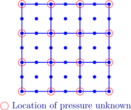
(a) Q2P1 interpolation for nine-node quadrilateral (Q9) element

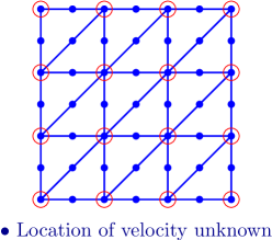
(b) P2P1 interpolation for six-node triangular (T6) element

Figure 1. This figure shows the typical structured finite element meshes employed in the current study. We use Q2P1 and P2P1 mixed interpolations to approximate the unknowns (i.e., second-order interpolation for the velocity field, and first-order interpolation for the pressure field).

We shall use several flow through porous media problems with different boundary conditions to illustrate that the proposed a posteriori techniques can be used as good measures for the accuracy and convergence of numerical results. We have employed P2P1 (which is based on six-node triangle element T6) and Q2P1 (which is based on nine-node quadrilateral element Q9) interpolations available in COMSOL [COM, 2013]. Consistent SUPG stabilization has been employed if the interpolations (i.e., Q2P1 and P2P1) violate the LBB inf-sup stability condition [Hughes et al., 1986; COM, 2013]. Typical structured finite elements utilized in this paper are shown in Figure 1. Unless mentioned otherwise, all the elements in a quadrilateral mesh are squares and all the elements in a triangular mesh are right-angled isosceles triangles. In this numerical solution study, we have taken $h$ (the maximum element size) to be equal to the length of the side for square elements, and to the length of the base (or height) for right-angled isosceles triangles.

4.1. Body force problem

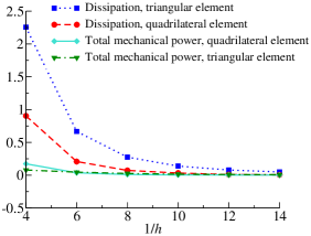
(a) Darcy model with $\mu=1$.

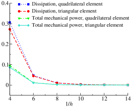
(b) Darcy-Brinkman model with $\mu=0.001$.

Figure 3. Body force problem: This figure shows the variation of the dissipation and the total mechanical power with mesh refinement under the Darcy and Darcy-Brinkman models using quadrilateral and triangular elements. The parameters used in this problem are provided in Table 1. The figure show that the total mechanical power and the dissipation decrease uniformly with mesh refinement, which are in accordance with Theorems 1 and 2.

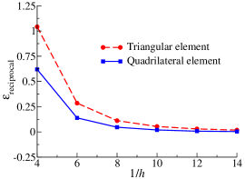
(a) Darcy model with $\mu=1$.

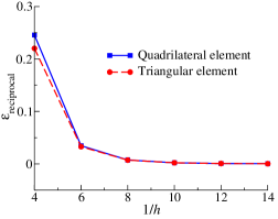
(b) Darcy-Brinkman model with $\mu=0.001$.

Figure 4. Body force problem: This figure shows the variation of $\varepsilon_{\mathrm{reciprocal}}$ with mesh refinement for the Darcy and Darcy-Brinkman models using quadrilateral and triangular elements. The parameters used in this problem is provided in Table 1. The figure show that the numerical error in the reciprocal relation decrease uniformly to zero with mesh refinement for this test problem.

The test problem is pictorially described in Figure 2. The non-dimensional parameters used in the numerical simulation are provided in Table 1. The conservative body force is taken as $\rho\mathbf{b}(\mathbf{x})=10[\mathrm{sin}(\pi x),\mathrm{cos}(\pi y)]$ (i.e., $a=10$). Velocity boundary condition is prescribed on the entire boundary (i.e., $\Gamma^{v}=\partial\Omega$). For the Darcy-Brinkman model, we assume $\mathbf{v}^{\mathrm{p}}(\mathbf{x})=\mathbf{0}$; and for the Darcy model, we assume $v_{n}(\mathbf{x})=0$. Figure 3 shows the minimum total mechanical power and the minimum dissipation with mesh refinement. The numerical results for the reciprocal relation with mesh refinement are shown in Figure 4. All the numerical results are in accordance with the theoretical predictions for this test problem.

Table 1. Body force problem: Non-dimensional parameters used in the problem.

Parameter	Value
$\alpha$	1
$\mu$	1 and 0.001
$\rho$	1
$L$	1
$\mathbf{b}(\mathbf{x})$	$a[\mathrm{sin}(\pi x),\mathrm{cos}(\pi y)]$

4.2. Lid-driven cavity problem

The two-dimensional lid-driven cavity problem is a benchmark study widely used to investigate the accuracy of numerical formulations for various fluid models [Burggraf, 1966; Erturk, 2009]. Figure 5 provides a pictorial description of the problem. The domain of the problem is a bi-unit square. Velocity boundary condition is prescribed on the entire boundary (i.e., $\Gamma^{v}=\partial\Omega$) which implies that the minimum dissipation theorem is also applicable to this problem. It should be noted that lid-driven cavity problem is not compatible with Darcy equations which need only the normal component of the velocity to be prescribed on the boundary. However, the lid-driven cavity problem demands the prescription of the entire velocity vector field on the boundary. We shall therefore employ Darcy-Brinkman model in our numerical simulations.

It is crucial to note that the solution to the lid-driven cavity problem has singularities at the top corners which arise due to velocity discontinuity on the boundary [Botella and Peyret, 1998; Batchelor, 2000].

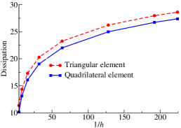
(c) Dissipation vs. $h$ under a hierarchy of uniform structured meshes.

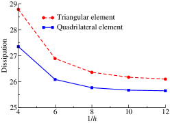
(d) Dissipation vs. $h$ under a hierarchy of adaptive meshes.

Figure 6. Lid-driven cavity problem: The top figures show a uniform structured mesh, and an adaptive mesh near the top corners. The bottom figures show the variation of total dissipation with mesh refinement for quadrilateral and triangular finite elements. The parameters in this problem are provided in Table 2. One should note that the solution exhibits singularities at the top corners. It is evident that the convergence is uniform under both structured and adaptive meshes. However, the dissipation under the structured mesh increased with mesh refinements, whereas the trend is reversed under the adaptive mesh. This is because the adaptive mesh resolves the singularities and removes the associated pollution error. This figure corroborates one of the main conclusions of the paper that the minimum dissipation theorem can be utilized to identify pollution errors in numerical solutions.

Herein, we use an adaptive mesh to resolve the singularities in the solution. The non-dimensional parameters used in the lid-driven cavity problem are presented in Table 2. Figures 6(a) and 6(b) show the uniform structured mesh and the adaptive mesh, respectively. For the adaptive mesh, we generate fine grid in the region close to top lid (see Figure 6(b)). Figures 6(c) and 6(d) show variation of the minimum dissipation with mesh refinement for respective grids. Under the adaptive mesh, the dissipation decreased uniformly and converged to a constant value with mesh refinement. On the other hand, the dissipation increased monotonically with mesh refinement under the structured mesh. More importantly, due to the presence of singularities and pollution error, the dissipation did not hit a plateau even for very fine meshes (i.e., $1/h\geq 220$). The dissipation reached a plateau relatively quickly under the adaptive mesh (say $1/h=10$). This problem clearly illustrates that the minimum dissipation theorem can be used to identify pollution errors and to check performance of adaptive mesh in numerical solutions which is one of the main findings of this paper.

Table 2. Lid-driven cavity problem: Non-dimensional parameters used in the problem.

Parameter	Value
$\alpha$	1
$\mu$	1
$\rho$	1
$L$	1

4.3. Pipe bend problem

As another application of the proposed techniques, we consider an engineering problem commonly found in the fluid mechanics literature, which is called the pipe bend problem (for example, see References [Borrvall and Petersson, 2003; Hansen et al., 2005; Aage et al., 2008; Pingen et al., 2009; Challis and Guest, 2009; Hassine, 2012]). In the pipe bend problem, the computational domain $\Omega$ is a square with $L=1$.

4.3.1. Velocity boundary condition

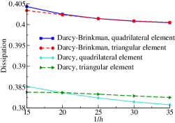
(a) Dissipation for $\alpha=10$.

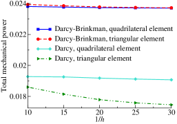
(b) Total mechanical power for $\alpha=1$.

Figure 8. Pipe bend problem (velocity boundary condition): The figure shows that the dissipation and total mechanical power decrease uniformly with mesh refinement for the Darcy and Darcy-Brinkman models. The results are presented for both quadrilateral and triangular elements. The parameters used in this problem are provided in Table 3 ($\mu=1$ for Darcy and $\mu=0.001$ for Darcy-Brinkman models). Note that the total mechanical power is defined in equation (3.5).

The problem is pictorially described in Figure 7. An inflow parabolic velocity is enforced on a part of the left boundary and an outflow parabolic velocity on a segment of the bottom. Each parabolic velocity profile has a unit maximum value (i.e., ${v}_{{x}_{max}}=1$ or ${v}_{{y}_{max}}=1$). Elsewhere, the homogeneous velocity is prescribed (i.e., $\mathbf{v}^{\mathrm{p}}(\mathbf{x})=\mathbf{0}$ for the Darcy-Brinkman model and $v_{n}(\mathbf{x})=0$ for the Darcy model). The velocity boundary condition makes the problem compatible with the total mechanical power and the dissipation theorems. The non-dimensional parameters used in the problem are presented in Table 3. Figure 8 shows the variation of minimum total mechanical power and minimum dissipation with mesh refinement for the quadrilateral and triangular elements. The result of the numerical solutions verification are presented in Figure 8(a) and 8(b) for the minimum dissipation and the total mechanical power, respectively. The numerical error decreases and converges uniformly.

4.3.2. Parabolic velocity-pressure boundary condition

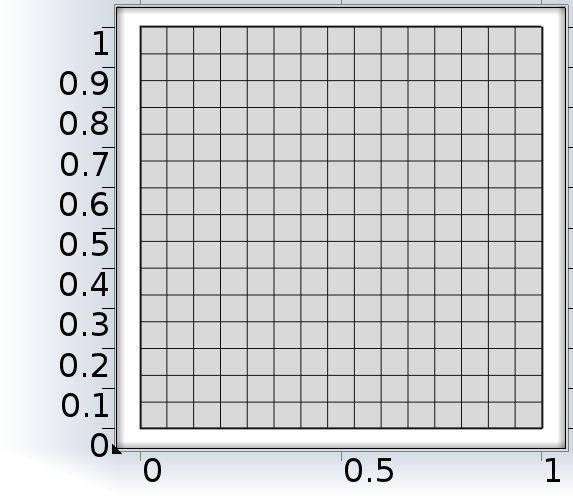
(a) Uniform structured mesh with $1/h=15$.

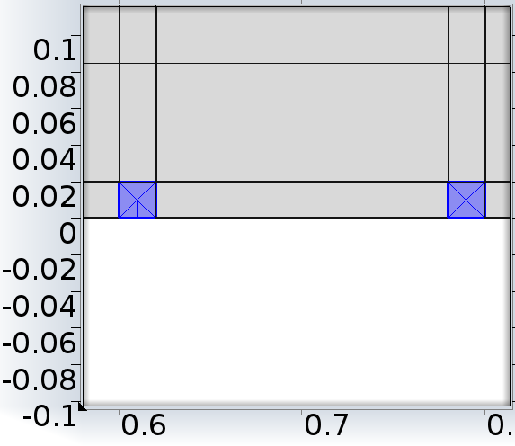
(b) Adaptive mesh near the outlet with $1/h=15$ elsewhere.

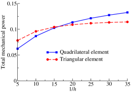
(c) Darcy-Brinkman model under the uniform structured mesh, $\mu=0.001$.

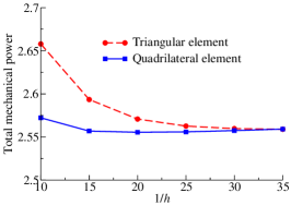
(d) Darcy-Brinkman model under the adaptive mesh, $\mu=0.001$.

Figure 10. Pipe bend problem (velocity-pressure boundary condition): The top figures show the uniform structured mesh and the adaptive mesh near the corners of the outlet (i.e., $\Gamma^{t}$). The bottom figures show the variation of the total mechanical power with mesh refinement under quadrilateral and triangular elements. The parameters used in this problem are provided in Table 3. The total mechanical power increased uniformly with mesh refinement under the structured mesh, while the total mechanical power decreased uniformly and reached a plateau with mesh refinement under the adaptive mesh. The numerical results clearly demonstrate that the total mechanical theorem can be utilized to identify pollution errors due to singularities and to assess whether a particular type of computational mesh is suitable for a given problem.

A pictorial description of the problem is given by Figure 9. The traction is prescribed on a part of the bottom boundary (i.e., $\mathbf{t}^{\mathrm{p}}(\mathbf{x})=-p_{\mathrm{atm}}\widehat{\mathbf{n}}(\mathbf{x})$ on $\Gamma^{t}$). The velocity has parabolic profile with unit maximum value (i.e., ${v}_{{x}_{max}}=1$) prescribed on a segment of the left boundary. Elsewhere, the homogeneous velocity is enforced. On account of the traction and parabolic velocity boundary conditions, current problem is not compatible with the minimum dissipation and reciprocal theorems. It is only compatible with the total mechanical power theorem. It should be noted that the solution to the problem has the singularity at near corners of the outlet (i.e., $\Gamma^{t}$). Hence, we again use an adaptive mesh to resolve the pollution in the solution. The non-dimensional parameters using in the problem are provided in Table 3. Figure 10 depicts the variation of the minimum total mechanical power with mesh refinement for the quadrilateral and triangular elements. The top figures show the uniform structured and adaptive meshes. Under the structured mesh, the total mechanical power increased uniformly with mesh refinement due to the polluted area in the computational domain. The error decreased uniformly and converged to a constant value with mesh refinement using the adaptive mesh. So, in addition to error estimation capability, the total mechanical power theorem can be used to identify the pollution errors in the numerical solutions and check the performance of adaptive mesh.

Table 3. Pipe bend problem: Non-dimensional parameters of the parabolic velocity boundary condition problem.

Parameter	Value
$\alpha$	1 and 10
$\mu$	1 and 0.001
$\rho$	1
$\mathbf{b}(\mathbf{x})$	[1, 1]
$L$	1

4.4. Pressure slab problem

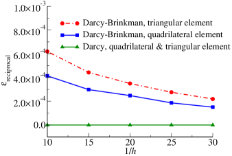
Figure 12. Pressure slab problem: The figure shows the variation of $\varepsilon_{\mathrm{reciprocal}}$ with mesh refinement for Darcy and Darcy-Brinkman equations using quadrilateral and triangular grids. The parameters in this problem are provided in Table 4. One can see the error in the numerical results with respect to the reciprocal relation for Darcy equations is very close to zero for all meshes. The corresponding error under Darcy-Brinkman equations decreases uniformly with mesh refinement.

Figure 11 provides a pictorial description of the problem. The non-dimensional parameters used in the numerical simulation are provided in Table 4. The domain is a $W\times L$ rectangle. The homogeneous velocity boundary condition is enforced on the top and bottom sides of the boundary. The traction is prescribed on the left side (i.e., $\mathbf{t}^{\mathrm{p}}(\mathbf{x})=-p_{\mathrm{inj}}\widehat{\mathbf{n}}(\mathbf{x})$ on $\Gamma^{t}_{1}$) and on the right side (i.e., $\mathbf{t}^{\mathrm{p}}(\mathbf{x})=-p_{\mathrm{atm}}\widehat{\mathbf{n}}(\mathbf{x})$ on $\Gamma^{t}_{2}$). We shall use this test problem to assess the accuracy of numerical solutions with respect to the reciprocal relation. Figure 12 depicts the variation of the error in the reciprocal relation with mesh refinement for the triangular and quadrilateral grids. The error in the reciprocal relations under Darcy equations is very close to zero for all the meshes. The error under Darcy-Brinkman equations decrease uniformly with mesh refinement. All the numerical results are in accordance with the theoretical predictions.

Table 4. Pressure slab problem: Non-dimensional parameters used in the problem.

Parameter	Value
$\alpha$	1
$\mu$	0.001
$\rho$	1
$p_{\mathrm{inj}}$	5 and 7.5
$p_{\mathrm{atm}}$	1
$L$	1
$W$	0.2

4.5. Pressure driven problem

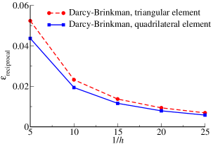
Figure 14. Pressure-driven problem:  Figure shows the variation of $\varepsilon_{\mathrm{reciprocal}}$ under the Darcy-Brinkman models using quadrilateral and triangular finite elements. The parameters used in this problem are provided in Table 5. Clearly, the reciprocal theorem can be utilized to obtain information on the numerical performance of the problem that does not possess an analytical solution.

The domain is a square with $L=1$. A pictorial description of the problem is given in Figure 13. The traction is prescribed on the left boundary (i.e., $\mathbf{t}^{\mathrm{p}}(\mathbf{x})=-p_{\mathrm{inj}}\widehat{\mathbf{n}}(\mathbf{x})$ on $\Gamma^{t}_{1}$) and on the middle of the right boundary (i.e., $\mathbf{t}^{\mathrm{p}}(\mathbf{x})=-p_{\mathrm{atm}}\widehat{\mathbf{n}}(\mathbf{x})$ on $\Gamma^{t}_{2}$). Elsewhere, homogeneous velocity boundary condition is enforced. Due to the prescription of the traction on a part of the boundary, this problem is incompatible with the minimum dissipation theorem but is compatible with the reciprocal relation and total mechanical power theorems. Herein, we present the results for the reciprocal relation. The non-dimensional parameters used in the numerical simulation are provided in Table 5. Figure 14 shows the variation of the error in the reciprocal relation with mesh refinement for triangular and quadrilateral meshes. The convergence under uniform structured meshes is uniformly to zero which is expected by theorem.

Table 5. Pressure driven problem: Non-dimensional parameters used in the problem.

Parameter	Value
$\alpha$	1
$\mu$	1 and 0.001
$\rho$	1
$p_{\mathrm{inj}}$	5 and 7.5
$p_{\mathrm{atm}}$	1
$L$	1

4.6. Vorticity results

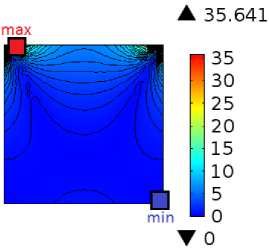
(a) Lid-driven cavity, regular mesh. $\omega_{max}=35.641$ and $\omega_{min}=0$.

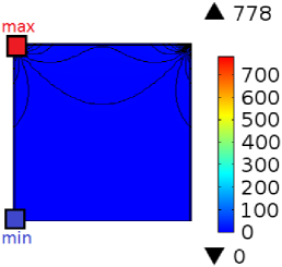
(b) Lid-driven cavity, adaptive mesh. $\omega_{max}=778$ and $\omega_{min}=0$.

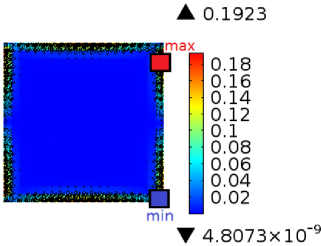
(c) Body force problem. $\omega_{max}=0.1923$ and $\omega_{min}=4.8073\times 10^{-9}$.

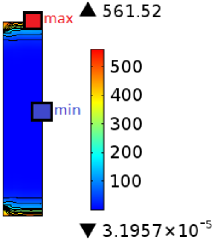
(d) Slab problem. $\omega_{max}=561.52$ and $\omega_{min}=3.1957\times 10^{-5}$.

Figure 15. The figure verifies the maximum principle for the vorticity for various two-dimensional problems under the Darcy-Brinkman model. We employed quadrilateral elements with size $1/h=20$. The numerical results corroborate the theoretical predictions given in Theorem 4 for all the test problems we have considered.

The maximum principle given by Theorem 4 can be used to assess the accuracy of numerical solutions to the Darcy-Brinkman equations by checking whether the non-negative maximum and non-positive minimum of the vorticity occur on the boundary. Figure 15 shows that the maximum principle is satisfied for various problems under the steady-state Darcy-Brinkman equations.

5. SYNTHETIC RESERVOIR DATA: MARMOUSI DATASET

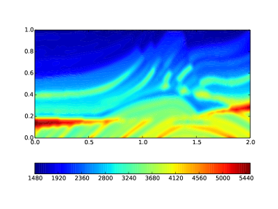
Figure 16. Synthetic reservoir problem: This figure shows the contours of (smooth) Marmousi dataset [Benamou, 2014]. The dataset provides values on a $384\times 122$ grid which we have scaled to our rectangular computational domain of $L=2$ and $H=1$. This spatially heterogeneous dataset is widely used as a benchmark dataset in reservoir modeling.

We will now solve an idealized reservoir problem using a popular synthetic dataset – the so-called (smooth) Marmousi dataset [Versteeg and Grau, 1990; Versteeg and Lailly, 1991; Versteeg, 1993; Klimes, 2014; Benamou, 2014]. The dataset provides spatially varying speed of sound on a $384\times 122$ grid. We have assumed that the permeability scales linearly with the values provided by the dataset. This is just an arbitrary choice to generate a heterogeneous dataset for permeability. However, it should be noted that the conclusions that will be drawn here will be valid even if one uses another dataset for the permeability. Figure 16 shows the contours of Marmousi dataset.

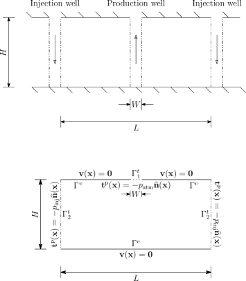
Figure 17. Synthetic reservoir problem: This figure provides a pictorial description of the test problem. The domain of the problem is a rectangle of size $H\times L$. The injection pressure is prescribed on the left and right boundaries (i.e., $\mathbf{t}^{\mathrm{p}}(\mathbf{x})=-p_{\mathrm{inj}}\widehat{\mathbf{n}}(\mathbf{x})\;\mathrm{on}\;\Gamma_{2}^{t}$), and the atmosphere pressure is prescribed on the middle of top side (i.e., $\mathbf{t}^{\mathrm{p}}(\mathbf{x})=-p_{\mathrm{atm}}\widehat{\mathbf{n}}(\mathbf{x})\;\mathrm{on}\;\Gamma_{1}^{t}$). The prescribed velocity on the remaining parts of the boundary is zero (i.e., $\mathbf{v}^{\mathrm{p}}(\mathbf{x})=\mathbf{0}$ for the Darcy-Brinkman model and $v_{n}(\mathbf{x})=0$ for the Darcy model).

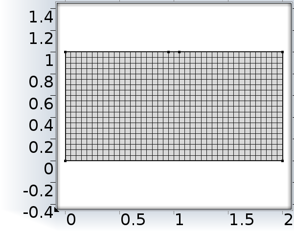
(a) Uniform structured mesh with $1/h=20$.

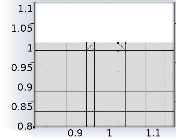
(b) Adaptive mesh near the production well with $1/h=20$ elsewhere.

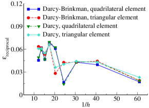
(c) Variation of $\varepsilon_{\mathrm{reciprocal}}$ under a hierarchy of uniform structured meshes.

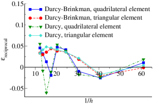
(d) Variation of $\varepsilon_{\mathrm{reciprocal}}$ under a hierarchy of adaptive meshes.

Figure 18. Synthetic reservoir problem: The figures show the variation of $\varepsilon_{\mathrm{reciprocal}}$ with $h$ for the Darcy and Darcy-Brinkman models using structured and adaptive meshes. The parameters in this problem are provided in Table 6. The figures clearly show that the errors in the reciprocal relation are larger under the uniform structured meshes. This can be attributed to pollution errors due to singularities at the corners of the production wells.

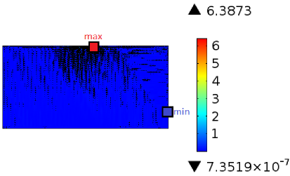
Figure 19. Synthetic reservoir problem: The figure shows the magnitude of vorticity for two-dimensional Darcy-Brinkman equations using quadrilateral elements. The parameters used in this problem are provided in Table 6. This figure verifies the maximum principle for the vorticity for the synthetic reservoir problem using Marmousi dataset.

The boundary value problem of the reservoir is pictorially described in Figure 17. This computational domain has been employed in some recent works (e.g., [Nakshatrala and Rajagopal, 2011]). All these works have assumed homogeneous medium properties, and did not use a reservoir data like the Marmousi dataset. Moreover, these studies did not address the use of a posteriori techniques to access numerical accuracy which is the main focus of the current paper. The parameters used in this problem are provided in Table 6. Figure 18 shows that the errors in the reciprocal relation are larger under uniform structured meshes than under adaptive meshes. This is due to the fact that uniform structured meshes suffer from pollution errors due to the singularity near the production well. The variation of the error in the reciprocal relation with mesh refinement provides guidelines on how much refinement is required to obtain solution of some desired accuracy especially in those cases where there are no analytical solutions. Figure 19 shows the magnitude of the vorticity, and one can see from the figure that the maximum principle for the vorticity is satisfied.

Table 6. Synthetic reservoir problem: Non-dimensional parameters used in the problem.

Parameter	Value
$\mu$	0.001
$\rho$	1
$p_{\mathrm{inj}}$	5 and 7.5
$p_{\mathrm{atm}}$	1
$L$	384
$H$	384/2
$W$	384$\times$0.1
$k$	Marmousi dataset/$L^{2}$

6. TRANSIENT CASE

6.1. Governing equations

Let us denote the time interval of interest by $\mathcal{I}$, and the time by $t\in\mathcal{I}$. The unsteady governing equations under the Darcy model take the following form:

$$\rho\frac{\partial\mathbf{v}}{\partial t}+\alpha\mathbf{v}+\mathrm{grad}[p]=\rho\mathbf{b}(\mathbf{x},t) \quad\mathrm{in}\;\Omega\times\mathcal{I}$$ (6.1a)

$$\mathrm{div}[\mathbf{v}]=0 \quad\mathrm{in}\;\Omega\times\mathcal{I}$$ (6.1b)

$$\mathbf{v}(\mathbf{x},t)\cdot\widehat{\mathbf{n}}(\mathbf{x})=v_{n}(\mathbf{x},t) \quad\mathrm{on}\;\Gamma^{v}\times\mathcal{I}$$ (6.1c)

$$p(\mathbf{x},t)=p_{0}(\mathbf{x},t) \quad\mathrm{on}\;\Gamma^{t}\times\mathcal{I}$$ (6.1d)

$$\mathbf{v}(\mathbf{x},t=0)=\mathbf{v}_{0}(\mathbf{x}) \quad\mathrm{in}\;\Omega$$ (6.1e)

Of course, the convective term $\mathrm{grad}[\mathbf{v}]\mathbf{v}$ is neglected. We assume that the coefficient of viscosity of the fluid and the permeability of the porous solid to be constants, and hence the drag coefficient is constant. We further assume that the density is homogeneous, and the body force is assumed to be conservative. The unsteady Darcy-Brinkman equations can be written as follows:

$$\rho\frac{\partial\mathbf{v}}{\partial t}+\alpha\mathbf{v}+\mathrm{grad}[p]-\mathrm{div}[2\mu\mathbf{D}]=\rho\mathbf{b}(\mathbf{x},t) \quad\mathrm{in}\;\Omega\times\mathcal{I}$$ (6.2a)

$$\mathrm{div}[\mathbf{v}]=0 \quad\mathrm{in}\;\Omega\times\mathcal{I}$$ (6.2b)

$$\mathbf{v}(\mathbf{x},t)=\mathbf{v}^{\mathrm{p}}(\mathbf{x},t) \quad\mathrm{on}\;\Gamma^{v}\times\mathcal{I}$$ (6.2c)

$$\mathbf{T}\widehat{\mathbf{n}}(\mathbf{x})=\mathbf{t}^{\mathrm{p}}(\mathbf{x},t) \quad\mathrm{on}\;\Gamma^{t}\times\mathcal{I}$$ (6.2d)

$$\mathbf{v}(\mathbf{x},t=0)=\mathbf{v}_{0}(\mathbf{x}) \quad\mathrm{in}\;\Omega$$ (6.2e)

where $\mathbf{v}^{\mathrm{p}}(\mathbf{x},t)$ is the prescribed velocity vector, and $\mathbf{t}^{\mathrm{p}}(\mathbf{x},t)$ is the prescribed traction.

6.2. Mathematical properties

Under unsteady Darcy equations, the vorticity satisfies the following equation:

$$\rho\frac{\partial\boldsymbol{\omega}}{\partial t}+\alpha\boldsymbol{\omega}=\boldsymbol{0}$$ (6.3)

which is an ordinary differential equation at each spatial point. The solution takes the following form:

$$\boldsymbol{\omega}(\mathbf{x},t)=\boldsymbol{\omega}_{0}(\mathbf{x})\exp\left[-\frac{\alpha t}{\rho}\right]$$ (6.4)

This means that the decay of vorticity should be exponential. One can check whether the numerical solutions exhibit this trend by plotting in log scale the each component of the vorticity with respect to time should, and this should be a straight line with slope $-\alpha/\rho$. If this trend is not satisfied for a given mesh and given time-step, does refining the grid spacing and the time-step improve the trend? Of course, one can check whether the vorticity goes to zero for large times. The vorticity under unsteady Darcy-Brinkman equations satisfies the following equation:

$$\rho\frac{\partial\boldsymbol{\omega}}{\partial t}+\alpha\boldsymbol{\omega}-\mu\Delta\boldsymbol{\omega}=\boldsymbol{0}\quad\mathrm{in}\;\Omega\times\mathcal{I}$$ (6.5)

where $\Delta$ is the Laplacian operator. The above equation is a homogeneous linear parabolic partial differential equation, which is known to satisfy a maximum principle [Pao, 1993]. This implies that both the maximum and the minimum will occur either in the initial condition or on the boundary. One can check whether numerical solutions satisfy the aforementioned maximum principle. Also, whether refining the grid spacing and time-steps affect the performance of numerical solutions with respect to this metric. One can devise any test problem as long as the following assumptions are met: (i) $\mu$ is constant, (ii) permeability is homogeneous, and (iii) the body force is conservative.

6.3. Representative numerical results

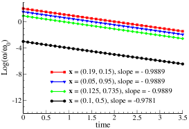
(a) Quadrilateral element size of $1/h=20$ for $dt=0.01$.

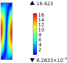
(b) Initial vorticity for quadrilateral element size of $1/h=20$.

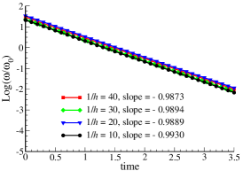
(c) Mesh refinement for quadrilateral elements, at $\mathbf{x}=(0.05,0.95)$ and $dt=0.01$.

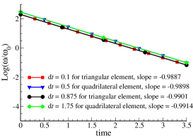
(d) Time refinement for $1/h=20$ at $\mathbf{x}=(0.15,0.35)$.

Figure 20. Pressure slab problem: The figure verifies the theoretical results for the vorticity under transient Darcy equations. The results show that the slope of $\log(\frac{\omega}{\omega_{0}})$ for various spatial points in the computational domain are close to $-\frac{\alpha}{\rho}=-1$. The figure also shows the slope is follows the theoretical prediction for various mesh refinements $h$ and time-steps $dt$. The non-dimensional parameters used in this numerical experiment are provided in Tables 4 and 7.

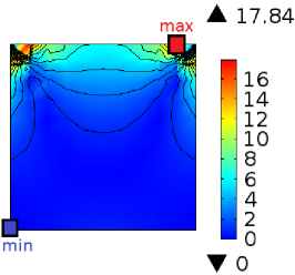
(a) Lid-driven cavity, structured mesh.

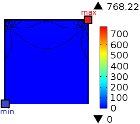
(b) Lid-driven cavity, adaptive mesh.

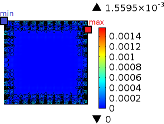
(c) Body force problem.

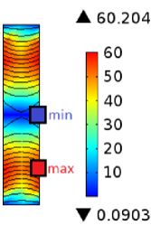
(d) Pressure slab problem.

Figure 21. The figure verifies the maximum principle for the vorticity under transient Darcy-Brinkman equations for various two-dimensional problems. The numerical results satisfy the maximum principle for all the test problems. The results are reported at $t=1$ and for time-step $dt=0.5$ (which is chosen arbitrarily). The results are presented for the adaptive and structured meshes based on quadrilateral elements with size $1/h=10$. We employed the backward Euler time-stepping scheme in the numerical experiment.

The theoretical results presented in this section are corroborated numerically in Figures 20–21. The vorticity results for the pressure slab problem under the transient Darcy model are provided in Figures 20. (Recall that Figure 11 provided a pictorial description of the pressure slab problem.) The non-dimensional parameters used in the numerical simulation are presented in Table 4, and the initial condition is provided in Table 7. Figure 20 shows that $\mathrm{log}(\frac{\omega}{\omega_{0}})$ is a straight line with slope equal to $\frac{\alpha}{\rho}$ under the mesh and time refinements for various spatial points in the solution of the transient Darcy equations (for the current problem $\frac{\alpha}{\rho}=-1$). Figure 21 verifies the maximum principle for vorticity for various test problems under transient Darcy-Brinkman equations. In all the cases, the non-negative maximum and non-positive minimum of the vorticity occur on the boundary, which agree with the mathematical theory presented above.

Table 7. Pressure slab problem: Initial condition used in the problem.

Parameter	Value
$p$	$p_{\mathrm{atm}}$
$v_{x}=v_{y}$	$\sin(\pi x/W)\sin(\pi y/L)$

7. CONCLUDING REMARKS

We presented a new methodology for solution verification which is independent of utilized numerical formulation. We called it mechanics-based solution verification. To employ this approach we developed four important properties (minimum dissipation theorem, minimum total mechanical power, reciprocal relation, and maximum principle for vorticity) that the solutions under the Darcy and the Darcy-Brinkman models satisfy. However, the proposed technique is not merely restricted to porous media type problems and one can easily extend it to other models. We also presented various test problems can serve as benchmark problems to verify numerical implementation of solvers for the Darcy and Darcy-Brinkman models. Results showed that the proposed technique can be effectively used to assess the accuracy of numerical solutions, identify numerical pollution, and check the performance of adaptive mesh. An attractive feature is that these properties can be verified for any given problem (i.e., needed not be one of the benchmark problems), and for any computational domain. For example, if the problem involves prescribing velocity boundary condition on the entire boundary, then one plots the dissipation with respect to mesh refinement. Some of the main conclusions are:

1. If the numerical formulation is converging, the dissipation, total mechanical power, and reciprocal relation should decrease with mesh refinement. If this does not occur, one needs to suspect that there are singularities in the solutions or that the numerical formulation does not perform well with respect to the local mass balance property.

2. It has been shown that the minimum dissipation, minimum total mechanical power, and reciprocal relation theorems can be utilized to identify pollution errors in numerical solutions. The theorems can also be used to assess whether a given type of mesh will be able to resolve singularities in the solution. This can be assessed by creating a series of hierarchical meshes and plotting for example the dissipation, with respect to characteristic mesh size. A given type of mesh will resolve singularities in the solution and will not be affected by pollution errors if the total dissipation decreases uniformly and reaches a plateau with a hierarchical mesh refinement.

3. The non-negative maximum vorticity and the non-positive minimum vorticity under Darcy-Brinkman equations with homogeneous isotropic medium properties should occur on the boundary.

4. Log plot of vorticity with respect to time, under transient Darcy models, is a line with slope $-\frac{\alpha}{\rho}$.

The proposed a posteriori techniques can be invaluable additions to the usual repertoire of methods for verification – the method of exact solutions (MES) and the method of manufactured solutions (MMS).

APPENDIX: UNIQUENESS OF SOLUTION

For completeness and pedagogical value, we now show that the uniqueness of solution under Darcy-Brinkman equations is a direct consequence of the minimum dissipation inequality. One can construct a proof for the uniqueness of solution under Darcy equations on similar lines.

Theorem 5 (Uniqueness theorem).

The solution to Darcy-Brinkman equations (2.4a)–(2.4d) is unique up to an arbitrary constant for the pressure given $\mathbf{b}(\mathbf{x})$, $\mathbf{v}^{\mathrm{p}}(\mathbf{x})$ and $\mathbf{t}^{\mathrm{p}}(\mathbf{x})$.

Proof.

On the contrary assume that $\left\{\mathbf{v}_{1}(\mathbf{x}),p_{1}(\mathbf{x})\right\}$ and $\left\{\mathbf{v}_{2}(\mathbf{x}),p_{2}(\mathbf{x})\right\}$ are two solutions to Darcy-Brinkman equations for the prescribed data. Let us consider the following quantity:

$$\mathcal{I}:=\int_{\Omega}\alpha(\mathbf{x})\left(\mathbf{v}_{1}(\mathbf{x})-\mathbf{v}_{2}(\mathbf{x})\right)\cdot\left(\mathbf{v}_{1}(\mathbf{x})-\mathbf{v}_{2}(\mathbf{x})\right)\;\mathrm{d}\Omega+\int_{\Omega}2\mu\left(\mathbf{D}_{1}(\mathbf{x})-\mathbf{D}_{2}(\mathbf{x})\right)\cdot\left(\mathbf{D}_{1}(\mathbf{x})-\mathbf{D}_{2}(\mathbf{x})\right)\;\mathrm{d}\Omega$$

Noting that $\mathrm{div}[\mathbf{v}_{1}]=0$ and $\mathrm{div}[\mathbf{v}_{2}]=0$, the second integral can be simplified as follows:

$$\int_{\Omega}2\mu\left(\mathbf{D}_{1}(\mathbf{x})-\mathbf{D}_{2}(\mathbf{x})\right)\cdot\left(\mathbf{D}_{1}(\mathbf{x})-\mathbf{D}_{2}(\mathbf{x})\right)\;\mathrm{d}\Omega =\int_{\Omega}\left(\mathbf{D}_{1}(\mathbf{x})-\mathbf{D}_{2}(\mathbf{x})\right)\cdot\left(\mathbf{T}_{1}(\mathbf{x})-\mathbf{T}_{2}(\mathbf{x})\right)\;\mathrm{d}\Omega$$

$$=\int_{\Omega}\mathrm{grad}\left[\mathbf{v}_{1}(\mathbf{x})-\mathbf{v}_{2}(\mathbf{x})\right]\cdot\left(\mathbf{T}_{1}(\mathbf{x})-\mathbf{T}_{2}(\mathbf{x})\right)\;\mathrm{d}\Omega$$

In obtaining the above equation, we have used the fact that $\mathbf{T}_{1}(\mathbf{x})$ and $\mathbf{T}_{2}(\mathbf{x})$ are symmetric. Using Green’s identity, the above equation can be written as follows:

$$\int_{\Omega}2\mu\left(\mathbf{D}_{1}(\mathbf{x})-\mathbf{D}_{2}(\mathbf{x})\right)\cdot\left(\mathbf{D}_{1}(\mathbf{x})-\mathbf{D}_{2}(\mathbf{x})\right)\;\mathrm{d}\Omega =\int_{\partial\Omega}(\mathbf{v}_{1}(\mathbf{x})-\mathbf{v}_{2}(\mathbf{x}))\cdot(\mathbf{T}_{1}(\mathbf{x})-\mathbf{T}_{2}(\mathbf{x}))\widehat{\mathbf{n}}(\mathbf{x})\;\mathrm{d}\Gamma$$

$$-\int_{\Omega}(\mathbf{v}_{1}(\mathbf{x})-\mathbf{v}_{2}(\mathbf{x}))\cdot(\mathrm{div}[\mathbf{T}_{1}]-\mathrm{div}[\mathbf{T}_{2}])\;\mathrm{d}\Omega$$

Using boundary conditions and the balance of linear momentum, we get the following:

$$\int_{\Omega}2\mu\left(\mathbf{D}_{1}(\mathbf{x})-\mathbf{D}_{2}(\mathbf{x})\right)\cdot\left(\mathbf{D}_{1}(\mathbf{x})-\mathbf{D}_{2}(\mathbf{x})\right)\;\mathrm{d}\Omega=-\int_{\Omega}\alpha(\mathbf{x})\left(\mathbf{v}_{1}(\mathbf{x})-\mathbf{v}_{2}(\mathbf{x})\right)\cdot\left(\mathbf{v}_{1}(\mathbf{x})-\mathbf{v}_{2}(\mathbf{x})\right)\;\mathrm{d}\Omega$$

This implies that $\mathcal{I}=0$. Since $\alpha(\mathbf{x})>0\;\forall\mathbf{x}\in\Omega$ and $\mu>0\;\mbox{in}\;\Omega$, one can conclude that

$$\mathbf{v}_{1}(\mathbf{x})=\mathbf{v}_{2}(\mathbf{x})\quad\forall\mathbf{x}\in\Omega$$ (7.1a)

$$\mathbf{D}_{1}(\mathbf{x})=\mathbf{D}_{2}(\mathbf{x})\quad\forall\mathbf{x}\in\Omega$$ (7.1b)

That is, the velocity and symmetric part of velocity vector field are unique. Using the equation for the balance of linear momentum (2.4a) and the fact that the velocity vector field is unique, one can obtain the following equation:

$$\mathrm{grad}\left[p_{1}(\mathbf{x})-p_{2}(\mathbf{x})\right]=\mathbf{0}\quad\forall\mathbf{x}\in\Omega$$ (7.2)

This further implies that

$$p_{1}(\mathbf{x})-p_{2}(\mathbf{x})=p_{0}\quad\forall\mathbf{x}\in\Omega$$ (7.3)

where $p_{0}$ is an arbitrary constant. This completes the proof. ∎

Figure 2. Body force problem:  The computational domain is a square with $L=1$. The prescribed conservative body force is $\rho\mathbf{b}(\mathbf{x})=10\times[\mathrm{sin}(\pi x),\mathrm{cos}(\pi y)]$. Homogeneous velocity is enforced on the entire boundary (i.e., $\Gamma^{v}=\partial\Omega$). That is, $\mathbf{v}^{\mathrm{p}}(\mathbf{x})=\mathbf{0}$ for Darcy-Brinkman equations and $v_{n}(\mathbf{x})=0$ for Darcy equations.

Figure 5. Lid-driven cavity problem: The computational domain is a unit square. Velocity boundary condition is prescribed on the entire boundary (i.e., $\Gamma^{v}=\partial\Omega$). The prescribed velocity on the top side is $v_{x}=1$ and $v_{y}=0$, and the prescribed velocity on the remaining sides of the boundary is zero (i.e., $\mathbf{v}^{\mathrm{p}}(\mathbf{x})=\mathbf{0}$). Note that this test problem is not compatible with Darcy equations.

(a) Uniform structured mesh with $1/h=12$.

(b) Adaptive mesh near the top left corner with $1/h=12$ elsewhere.

Figure 7. Pipe bend problem (velocity boundary condition): A pictorial description of the problem. The computational domain $\Omega$ is a unit square. The velocity boundary condition is prescribed on the entire boundary (i.e., $\Gamma^{v}=\partial\Omega$). As indicated in the figure, a parabolic velocity profile with $v_{x_{max}}=1$ is prescribed on a segment of the left side of the boundary. Similarly, a parabolic velocity profile with $v_{y_{max}}=1$ is prescribed on a segment of the bottom side of the boundary. Homogeneous velocity is enforced on the remaining parts of the boundary.

Figure 9. Pipe bend problem (velocity-pressure boundary condition): This figure presents a pictorial description of the problem. The computational domain $\Omega$ is a square with $L=1$. The traction boundary condition is $\mathbf{t}^{\mathrm{p}}(\mathbf{x})=-p_{\mathrm{atm}}\widehat{\mathbf{n}}(\mathbf{x})\;\mathrm{on}\;\Gamma^{t}$. A parabolic velocity profile with ${v}_{{x}_{max}}=1$ is prescribed on a segment of the left side of the boundary, as indicated in the figure. Elsewhere, the velocity is assumed to be zero (i.e., $\mathbf{v}^{\mathrm{p}}(\mathbf{x})=\mathbf{0}$ for Darcy-Brinkman equations and $v_{n}(\mathbf{x})=0$ for Darcy equations). Note that the corners at the outlet are re-entrant corners.

Figure 11. Pressure slab problem: A pictorial description of the problem. The computational domain is a $W\times L$ rectangle. The traction is prescribed on the left side of the boundary (i.e., $\mathbf{t}^{\mathrm{p}}(\mathbf{x})=-p_{\mathrm{inj}}\widehat{\mathbf{n}}(\mathbf{x})$ on $\Gamma^{t}_{1}$) and on the right side (i.e., $\mathbf{t}^{\mathrm{p}}(\mathbf{x})=-p_{\mathrm{atm}}\widehat{\mathbf{n}}(\mathbf{x})$ on $\Gamma^{t}_{2}$). Elsewhere, homogeneous velocity is enforced.

Figure 13. Pressure-driven problem:  A pictorial description of the problem. The computational domain $\Omega$ is a square with $L=1$. The traction is prescribed on the left side of the boundary (i.e., $\mathbf{t}^{\mathrm{p}}(\mathbf{x})=-p_{\mathrm{inj}}\widehat{\mathbf{n}}(\mathbf{x})$ on $\Gamma^{t}_{1}$) and on the middle of right side (i.e., $\mathbf{t}^{\mathrm{p}}(\mathbf{x})=-p_{\mathrm{atm}}\widehat{\mathbf{n}}(\mathbf{x})$ on $\Gamma^{t}_{2}$). Elsewhere, homogeneous velocity is enforced.

References

- COM [2013] COMSOL Multiphysics User’s Guide, Version 4.3b. COMSOL, Inc., Burlington, Massachusetts, www.comsol.com, 2013.
- Aage et al. [2008] N. Aage, T. H. Poulsen, A. G. Hansen, and O. Sigmund. Topology optimization of large scale Stokes flow problems. Structural and Multidisciplinary Optimization, 35:175–180, 2008.
- Ainsworth and Oden [1997] M. Ainsworth and J. T. Oden. A posteriori error estimation in finite element analysis. Computer Methods in Applied Mechanics and Engineering, 142:1–88, 1997.
- Babuška and Oden [2004] I. Babuška and J. T. Oden. Verification and validation in computational engineering and science: basic concepts. Computer Methods in Applied Mechanics and Engineering, 193:4057–4066, 2004.
- Babuška and Oh [1987] I. Babuška and H.-S. Oh. Pollution problem of the p- and h-p versions of the finite element method. Communications in Applied Numerical Methods, 3:553–561, 1987.
- Babuška and Strouboulis [2001] I. Babuška and T. Strouboulis. The Finite Element Method and its Reliability. Oxford University Press, Oxford, 2001.
- Babuška et al. [1995] I. Babuška, T. Strouboulis, C. S. Upadhyay, and S. K. Gangaraj. A posteriori estimation and adaptive control of the pollution error in the h-version of the finite element method. International Journal for Numerical Methods in Engineering, 38:4207–4235, 1995.
- Babuška et al. [1997] I. Babuška, F. Ihlenburg, T. Strouboulis, and S. K. Gangaraj. A posteriori error estimation for finite element solutions of Helmholtz equation-Part II: Estimation of the pollution error. International Journal for Numerical Methods in Engineering, 40:3883–3900, 1997.
- Batchelor [2000] G. K. Batchelor. An Introduction to Fluid Dynamics. Cambridge University Press, New York, 2000.
- Becker and Rannacher [2001] R. Becker and R. Rannacher. An optimal control approach to a posteriori error estimation in finite element methods. Acta Numerica, 10:1–102, 2001.
- Benamou [2014] J.-D. Benamou. Computation of MULTI-VALUED TRAVELTIMES in the Marmousi model, 2014. URL http://www.caam.rice.edu/ benamou/testproblem.html.
- Blottner [1990] F. G. Blottner. Accurate Navier-Stokes results for the hypersonic flow over a spherical nosetip. Journal Spacecraft and Rockets, 27:113–122, 1990.
- Borrvall and Petersson [2003] T. Borrvall and J. Petersson. Topology optimization of fluids in Stokes flow. International Journal for Numerical Methods in Fluids, 41:77–107, 2003.
- Botella and Peyret [1998] O. Botella and R. Peyret. Benchmark spectral results on the lid-driven cavity flow. Computers and Fluids, 27:421–433, 1998.
- Botella and Peyret [2001] O. Botella and R. Peyret. Computing singular solutions of the Navier-Stokes equations with the Chebyshev-collocation method. International Journal for Numerical Methods in Fluids, 36:125–163, 2001.
- Brezzi and Fortin [1991] F. Brezzi and M. Fortin. Mixed and Hybrid Finite Element Methods, volume 15 of Springer series in computational mathematics. Springer-Verlag, New York, 1991.
- Brinkman [1947a] H. C. Brinkman. A calculation of the viscous force exerted by a flowing fluid on a dense swarm of particles. Applied Scientific Research, A1:27–34, 1947a.
- Brinkman [1947b] H. C. Brinkman. On the permeability of the media consisting of closely packed porous particles. Applied Scientific Research, A1:81–86, 1947b.
- Burggraf [1966] O. R. Burggraf. Analytical and numerical studies of the structure of steady separated flows. Journal of Fluid Mechanics, 24:113–151, 1966.
- Challis and Guest [2009] V. J. Challis and J. K. Guest. Level set topology optimization of fluids in Stokes flow. International Journal for Numerical Methods in Engineering, 79:1284–1308, 2009.
- Darcy [1856] H. Darcy. Les Fontaines Publiques de la Ville de Dijon. Victor Dalmont, Paris, 1856.
- Erturk [2009] E. Erturk. Discussions on driven cavity flow. International Journal for Numerical Methods in Fluids, 60:275–294, 2009.
- Evans [1998] L. C. Evans. Partial Differential Equations. American Mathematical Society, Providence, Rhode Island, 1998.
- Gilbarg and Trudinger [2001] D. Gilbarg and N. S. Trudinger. Elliptic Partial Differential Equations of Second Order. Springer, New York, 2001.
- Guazzelli and Morris [2012] E. Guazzelli and J. F. Morris. A Physical Introduction to Suspension Dynamics. Cambridge University Press, Cambridge, 2012.
- Hansen et al. [2005] A. G. Hansen, O. Sigmund, and R. B. Haber. Topology optimization of channel flow problems. Structural and Multidisciplinary Optimization, 30:181–192, 2005.
- Hassine [2012] M. Hassine. Topology Optimization of Fluid Mechanics Problems. In S. A. Jones, editor, Advanced Methods for Practical Applications in Fluid Mechanics, pages 209–230. InTech, 2012.
- Hughes et al. [1986] T. J. R. Hughes, L. Franca, and M. Balestra. A new finite element formulation for computational fluid dynamics: V. Circumventing the Babuska-Brezzi condition: A stable Petrov-Galerkin formulation of the Stokes problem accommodating equal-order interpolations. Computer Methods in Applied Mechanics and Engineering, 59:85–99, 1986.
- Kellogg [2010] O. D. Kellogg. Foundations of Potential Theory. Dover Publications, New York, 2010.
- Klimes [2014] L. Klimes. Seismic Waves in Complex 3-D Structures (SW3D), Marmousi model and data set, Department of Geophysics, Charles University in Prague, 2014. URL http://seis.karlov.mff.cuni.cz/software/marmousi/marmousi.htm.
- Knupp and Salari [2003] P. M. Knupp and K. Salari. Verification of Computer Codes in Computational Science and Engineering. Chapman & Hall/CRC, Boca Raton, 2003.
- Masud and Hughes [2002] A. Masud and T. J. R. Hughes. A stabilized mixed finite element method for Darcy flow. Computer Methods in Applied Mechanics and Engineering, 191:4341–4370, 2002.
- Mudunuru and Nakshatrala [2016] M. K. Mudunuru and K. B. Nakshatrala. On enforcing maximum principles and achieving element-wise species balance for advection–diffusion–reaction equations under the finite element method. Journal of Computational Physics, 305:448–493, 2016.
- Nakshatrala and Rajagopal [2011] K. B. Nakshatrala and K. R. Rajagopal. A numerical study of fluids with pressure-dependent viscosity flowing through a rigid porous medium. International Journal for Numerical Methods in Fluids, 67:342–368, 2011.
- Nakshatrala et al. [2006] K. B. Nakshatrala, D. Z. Turner, K. D. Hjelmstad, and A. Masud. A stabilized mixed finite element formulation for Darcy flow based on a multiscale decomposition of the solution. Computer Methods in Applied Mechanics and Engineering, 195:4036–4049, 2006.
- Nakshatrala et al. [2015] K. B. Nakshatrala, H. Nagarajan, and M. Shabouei. A numerical methodology for enforcing maximum principles and the non-negative constraint for transient diffusion equations. doi: 10.4208/cicp.180615.280815a, 2015.
- Oberkampf and Blottner [1998] W. L. Oberkampf and F. G. Blottner. Issues in computational fluid dynamics: Code verification and validation. AIAA Journal, 36:687–695, 1998.
- Oberkampf et al. [2004] W. L. Oberkampf, T. G. Trucano, and C. Hirsch. Verification, validation, and predictive capability in computational engineering and physics. Applied Mechanics Reviews, 57:345–384, 2004.
- Oden et al. [1998] J. T. Oden, Y. Feng, and S. Prudhomme. Local and pollution error estimation for Stokesian flows. International Journal for Numerical Methods in Fluids, 27:33–39, 1998.
- Pao [1993] C. V. Pao. Nonlinear Parabolic and Elliptic Equations. Springer-Verlag, New York, USA, 1993.
- Pingen et al. [2009] G. Pingen, A. Evgrafov, and K. Maute. Adjoint parameter sensitivity analysis for the hydrodynamic lattice Boltzmann method with applications to design optimization. Computers and Fluids, 38:910–923, 2009.
- Rider et al. [2016] W. Rider, W. Witkowski, J. R. Kamm, and T. Wildey. Robust verification analysis. Journal of Computational Physics, 307:146–163, 2016.
- Roache [1997] P. J. Roache. Quantification of uncertainty in computational fluid dynamics. Annual Review of Fluid Mechanics, 29:123–160, 1997.
- Roache [1998] P. J. Roache. Verification and Validation in Computational Science and Engineering. Hermosa Publishers, New Mexico, 1998.
- Roy et al. [2004] C. J. Roy, C. C. Nelson, T. M. Smith, and C. C. Ober. Verification of Euler/Navier-–Stokes codes using the method of manufactured solutions. International Journal for Numerical Methods in Fluids, 44:599–620, 2004.
- Sadd [2009] M. H. Sadd. Elasticity: Theory, Applications, and Numerics. Academic Press, Burlington, Massachusetts, 2009.
- Salari and Knupp [2000] K. Salari and P. M. Knupp. Code Verification by the Method of Manufactured Solutions. Technical Report SAND2000-1444, Sandia National Laboratories, Albuquerque, 2000.
- Truesdell and Noll [2004] C. Truesdell and W. Noll. The Non-Linear Field Theories of Mechanics. Springer, Berlin, third edition, 2004.
- Versteeg [1993] R. J. Versteeg. Sensitivity of prestack depth migration to the velocity model. Geophysics, 58:873–882, 1993.
- Versteeg and Grau [1990] R. J. Versteeg and G. Grau. The Marmousi experience. In Practical aspects of seismic data inversion, European Association of Exploration Geophysicists, EAEG Workshop, 52nd EAEG Meeting, pages 1–194, Copenhagen, 1990.
- Versteeg and Lailly [1991] R. J. Versteeg and P. Lailly. In Practical aspects of seismic data inversion, European Association of Exploration Geophysicists, EAEG workshop report: First Break, pages 75–80, 1991.