Shield Synthesis:

Abstract

Scalability issues may prevent users from verifying critical properties of a complex hardware design. In this situation, we propose to synthesize a “safety shield” that is attached to the design to enforce the properties at run time. Shield synthesis can succeed where model checking and reactive synthesis fail, because it only considers a small set of critical properties, as opposed to the complex design, or the complete specification in the case of reactive synthesis. The shield continuously monitors the input/output of the design and corrects its erroneous output only if necessary, and as little as possible, so other non-critical properties are likely to be retained. Although runtime enforcement has been studied in other domains such as action systems, reactive systems pose unique challenges where the shield must act without delay. We thus present the first shield synthesis solution for reactive hardware systems and report our experimental results. This is an extended version of [5], featuring an additional appendix.

1 Introduction

Model checking [10, 18] can formally verify that a design satisfies a temporal logic specification. Yet, due to scalability problems, it may be infeasible to prove all critical properties of a complex design. Reactive synthesis [17, 4] is even more ambitious since it aims to generate a provably correct design from a given specification. In addition to scalability problems, reactive synthesis has the drawback of requiring a complete specification, which describes every aspect of the desired design. However, writing a complete specification can sometimes be as hard as implementing the design itself.

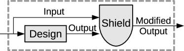
Figure 1: Attaching a safety shield.

We propose shield synthesis as a way to complement model checking and reactive synthesis. Our goal is to enforce a small set of critical properties at runtime even if these properties may occasionally be violated by the design. Imagine a complex design and a set of properties that cannot be proved due to scalability issues or other reasons (e.g., third-party IP cores). In this setting, we are in good faith that the properties hold but we need to have certainty. We would like to automatically construct a component, called the shield, and attach it to the design as illustrated in Fig. 1. The shield monitors the input/output of the design and corrects the erroneous output values instantaneously, but only if necessary and as little as possible.

The shield ensures both correctness and minimum interference. By correctness, we mean that the properties must be satisfied by the combined system, even if they are occasionally violated by the design. By minimum interference, we mean that the output of the shield deviates from the output of the design only if necessary, and the deviation is kept minimum. The latter requirement is important because we want the design to retain other (non-critical) behaviors that are not captured by the given set of properties. We argue that shield synthesis can succeed even if model checking and reactive synthesis fail due to scalability issues, because it has to enforce only a small set of critical properties, regardless of the implementation details of a complex design.

This paper makes two contributions. First, we define a general framework for solving the shield synthesis problem for reactive hardware systems. Second, we propose a new synthesis method, which automatically constructs a shield from a set of safety properties. To minimize deviations of the shield from the original design, we propose a new notion called $k$-stabilization: When the design arrives at a state where a property violation becomes unavoidable for some possible future inputs, the shield is allowed to deviate for at most $k$ consecutive steps. If a second violation happens during the $k$-step recovery phase, the shield enters a fail-safe mode where it only enforces correctness, but no longer minimizes the deviation. We show that the $k$-stabilizing shield synthesis problem can be reduced to safety games [15]. Following this approach, we present a proof-of-concept implementation and give the first experimental results.

Our work on shield synthesis can complement model checking by enforcing any property that cannot be formally proved on a complex design. There can be more applications. For example, we may not trust third-party IP components in our system, but in this case, model checking cannot be used because we do not have the source code. Nevertheless, a shield can enforce critical interface assumptions of these IP components at run time. Shields may also be used to simplify certification. Instead of certifying a complex design against critical requirements, we can synthesize a shield to enforce them, regardless of the behavior of the design. Then, we only need to certify this shield, or the synthesis procedure, against the critical requirements. Finally, shield synthesis is a promising new direction for synthesis in general, because it has the strengths of reactive synthesis while avoiding its weaknesses — the set of critical properties can be small and relatively easy to specify — which implies scalability and usability.

Related work. Shield synthesis is different from recent works on reactive synthesis [17, 4, 12], which revisited Church’s problem [9, 8, 19] on constructing correct systems from logical specifications. Although there are some works on runtime enforcement of properties in other domains [20, 14, 13], they are based on assumptions that do not work for reactive hardware systems. Specifically, Schneider [20] proposed a method that simply halts a program in case of a violation. Ligatti et al. [14] used edit automata to suppress or insert actions, and Falcone et al. [13] proposed to buffer actions and dump them once the execution is shown to be safe. None of these approaches is appropriate for reactive systems where the shield must act upon erroneous outputs on-the-fly, i.e., without delay and without knowing what future inputs/outputs are. In particular, our shield cannot insert or delete time steps, and cannot halt in the case of a violation.

Methodologically, our new synthesis algorithm builds upon the existing work on synthesis of robust systems [3], which aims to generate a complete design that satisfies as many properties of a specification as possible if assumptions are violated. However, our goal is to synthesize a shield component $S$, which can be attached to any design $D$, to ensure that the combined system $(S\circ D)$ satisfies a given set of critical properties. Our method aims at minimizing the ratio between shield deviations and property violations by the design, but achieves it by solving pure safety games. Furthermore, the synthesis method in [3] uses heuristics and user input to decide from which state to continue monitoring the environmental behavior, whereas we use a subset construction to capture all possibilities to avoid unjust verdicts by the shield. We use the notion of $k$-stabilization to quantify the shield deviation from the design, which has similarities to Ehlers and Topcu’s notion of $k$-resilience in robust synthesis [12] for GR(1) specifications [4]. However, the context of our work is different, and our $k$-stabilization limits the length of the recovery period instead of tolerating bursts of up to $k$ glitches.

Outline. The remainder of this paper is organized as follows. We illustrate the technical challenges and our solutions in Section 2 using an example. Then, we establish notation in Section 3. We formalize the problem in a general framework for shield synthesis in Section 4, and present our new method in Section 5. We present our experimental results in Section 6 and, finally, give our conclusions in Section 7.

2 Motivation

In this section, we illustrate the challenges associated with shield synthesis and then briefly explain our solution using an example. We start with a traffic light controller that handles a single crossing between a highway and a farm road. There are red (r) or green (g) lights for both roads. An input signal, denoted $\textsf{p}\in\{0,1\}$, indicates whether an emergency vehicle is approaching. The controller takes p as input and returns h,f as output. Here, $\textsf{h}\in\{r,g\}$ and $\textsf{f}\in\{r,g\}$ are the lights for highway and farm road, respectively. Although the traffic light controller interface is simple, the actual implementation can be complex. For example, the controller may have to be synchronized with other traffic lights, and it can have input sensors for cars, buttons for pedestrians, and sophisticated algorithms to optimize traffic throughput and latency based on all sensors, the time of the day, and even the weather. As a result, the actual design may become too complex to be formally verified. Nevertheless, we want to ensure that a handful of safety critical properties are satisfied with certainty. Below are three example properties:

1. The output gg — meaning that both roads have green lights — is never allowed.

2. If an emergency vehicle is approaching ($\textsf{p}=1$), the output must be rr.

3. The output cannot change from gr to rg, or vice versa, without passing rr.

We want to synthesize a safety shield that can be attached to any implementation of this traffic light controller, to enforce these properties at run time.

In a first exercise, we only consider enforcing Properties 1 and 2. These are simple invariance properties without any temporal aspects. Such properties can be represented by a truth table as shown in Fig. 2 (left). We use 0 to encode r, and 1 to encode g. Forbidden behavior is marked in bold red. The shield must ensure both correctness and minimum interference. That is, it should only change the output for red entries.

p	h	f	h’	f’
0	0	0	0	0
0	0	1	0	1
0	1	0	1	0
0	1	1	1	0
1	0	0	0	0
1	0	1	0	0
1	1	0	0	0
1	1	1	0	0

$\Rightarrow$ $\mathsf{h^{\prime}=\neg p\wedge h}$ $\mathsf{f^{\prime}=\neg p\wedge\neg h\wedge f}$

Figure 2: Enforcing Properties 1 and 2.

In particular, it should not ignore the design and hard-wire the output to rr. When $\mathsf{p=1}$ but the output is not $\mathsf{rr}$, the shield must correct the output to $\mathsf{rr}$. When $\mathsf{p=0}$ but the output is gg, the shield must turn the original output gg into either rg, gr, or rr. Assume that gr is chosen. As illustrated in Fig. 2 (right), we can construct the transition functions $h^{\prime}=\neg p\wedge h$ and $f^{\prime}=\neg p\wedge\neg h\wedge f$, as well as the shield circuit accordingly.

Next, we consider enforcing Properties 1–3 together. Property 3 brings in a temporal aspect, so a simple truth table does not suffice any more. Instead, we express the properties by an automaton, which is shown in Fig. 3. Edges are labeled by values of phf, where $\mathsf{p}\in\{0,1\}$ is the controller’s input and $\mathsf{h,f}$ are outputs for highway and farm road.

Figure 3: Traffic light specification.

There are three non-error states: H denotes the state where highway has the green light, F denotes the state where farm road has the green light, and B denotes the state where both have red lights. There is also an error state, which is not shown. Missing edges lead to this error state, denoting forbidden situations, e.g., 1gr is not allowed in state H. Although the automaton still is not a complete specification, the corresponding shield can prevent catastrophic failures. By automatically generating a small shield as shown in Fig. 1, our approach has the advantage of combining the functionality and performance of the aggressively optimized implementation with guaranteed safety.

While the shield for Property 1 and 2 could be realized by purely combinational logic, this is not possible for the specification in Fig. 3. The reason is the temporal aspect brought in by Property 3. For example, if we are in state F and observe 0gg, which is not allowed, the shield has to make a correction in the output signals to avoid the violation. There are two options: changing the output from gg to either rg or rr. However, this fix may result in the next state being either B or F. The question is, without knowing what the future inputs/outputs are, how do we decide from which state the shield should continue to monitor the behavior of the design in order to best detect and correct future violations? If the shield makes a wrong guess now, it may lead to a suboptimal implementation that causes unnecessarily large deviation in the future.

To solve this problem, we adopt the most conservative approach. That is, we assume that the design $\mathcal{D}$ meant to give one of the allowed outputs, so either rr or rg. Thus, our shield continues to monitor the design from both F and B. Technically, this is achieved by a form of subset construction (see Sec. 5.2), which tracks all possibilities for now, and then gradually refines its knowledge with future observations. For example, if the next observation is 0gr, we assume that the design $\mathcal{D}$ meant rr earlier, and so it must be in B and traverse to H. If it were in F, we could only have explained 0gr by assuming a second violation, which is less optimistic than we would like to be. In this work, we assume that a second violation occurs only if an observation is inconsistent with all states that it could possibly be in. For example, if the next observation is not 0gr but 1rg, which is neither allowed in F nor in B, we know that a second violation occurs. Yet, after observing 1rg, we can be sure that we have reached the state B, because starting from both F and B, with input $\textsf{p}=1$, the only allowed output is rr, and the next state is always B. In this sense, our construction implements an “innocent until proved guilty” philosophy, which is key to satisfy the minimum interference requirement.

To bound the deviation of the shield when a property violation becomes unavoidable, we require the shield to deviate for at most $k$ consecutive steps after the initial violation. We shall formalize this notion of $k$-stabilization in subsequent sections and present our synthesis algorithm. For the safety specification in Fig. 3, our method would reduce the shield synthesis problem into a set of safety games, which are then solved using standard techniques (cf. [15]). We shall present the synthesis results in Section 6.

3 Preliminaries

We denote the Boolean domain by $\mathbb{B}=\{\mathsf{true},\mathsf{false}\}$, denote the set of natural numbers by $\mathbb{N}$, and abbreviate $\mathbb{N}\cup\{\infty\}$ by $\mathbb{N}^{\infty}$. We consider a reactive system with a finite set $I=\{i_{1},\ldots,i_{m}\}$ of Boolean inputs and a finite set $O=\{o_{1},\ldots,o_{n}\}$ of Boolean outputs. The input alphabet is $\Sigma_{I}=2^{I}$, the output alphabet is $\Sigma_{O}=2^{O}$, and $\Sigma=\Sigma_{I}\times\Sigma_{O}$. The set of finite (infinite) words over $\Sigma$ is denoted by $\Sigma^{*}$ ($\Sigma^{\omega}$), and $\Sigma^{*,\omega}=\Sigma^{*}\cup\Sigma^{\omega}$. We will also refer to words as (execution) traces. We write $|\overline{\sigma}|$ for the length of a trace $\overline{\sigma}\in\Sigma^{*,\omega}$. For ${\overline{\sigma_{I}}}=x_{0}x_{1}\ldots\in\Sigma_{I}^{\omega}$ and ${\overline{\sigma_{O}}}=y_{0}y_{1}\ldots\in\Sigma_{O}^{\omega}$, we write ${\overline{\sigma_{I}}}||{\overline{\sigma_{O}}}$ for the composition $(x_{0},y_{0})(x_{1},y_{1})\ldots\in\Sigma^{\omega}$. A set $L\subseteq\Sigma^{\omega}$ of infinite words is called a language. We denote the set of all languages as $\mathcal{L}=2^{\Sigma^{\omega}}$.

Reactive Systems. A reactive system $\mathcal{D}=(Q,q_{0},\Sigma_{I},\Sigma_{O},\delta,\lambda)$ is a Mealy machine, where $Q$ is a finite set of states, $q_{0}\in Q$ is the initial state, $\delta:Q\times\Sigma_{I}\rightarrow Q$ is a complete transition function, and $\lambda:Q\times\Sigma_{I}\rightarrow\Sigma_{O}$ is a complete output function. Given the input trace ${\overline{\sigma_{I}}}=x_{0}x_{1}\ldots\in\Sigma_{I}^{\omega}$, the system $\mathcal{D}$ produces the output trace ${\overline{\sigma_{O}}}=\mathcal{D}({\overline{\sigma_{I}}})=\lambda(q_{0},x_{0})\lambda(q_{1},x_{1})\ldots\in\Sigma_{O}^{\omega}$, where $q_{i+1}=\delta(q_{i},x_{i})$ for all $i\geq 0$. The set of words produced by $\mathcal{D}$ is denoted $L(\mathcal{D})=\{{\overline{\sigma_{I}}}||{\overline{\sigma_{O}}}\in\Sigma^{\omega}\mid\mathcal{D}({\overline{\sigma_{I}}})={\overline{\sigma_{O}}}\}$. We also refer to a reactive system $\mathcal{D}$ as a (hardware) design.

Let $\mathcal{D}=(Q,q_{0},\Sigma_{I},\Sigma_{O},\delta,\lambda)$ and $\mathcal{D}^{\prime}=(Q^{\prime},q_{0}^{\prime},\Sigma,\Sigma_{O},\delta^{\prime},\lambda^{\prime})$ be reactive systems. Their serial composition is constructed by feeding the input and output of $\mathcal{D}$ to $\mathcal{D}^{\prime}$ as input. We use $\mathcal{D}\circ\mathcal{D}^{\prime}$ to denote such a composition $(\hat{Q},\hat{q_{0}},\Sigma_{I},\Sigma_{O},\hat{\delta},\hat{\lambda})$, where $\hat{Q}=Q\times Q^{\prime}$, $\hat{q_{0}}=(q_{0},q_{0}^{\prime})$, $\hat{\delta}((q,q^{\prime}),{\sigma_{I}})=(\delta(q,{\sigma_{I}}),\delta^{\prime}(q^{\prime},({\sigma_{I}},\lambda(q,{\sigma_{I}}))))$, and $\hat{\lambda}((q,q^{\prime}),{\sigma_{I}})=\lambda^{\prime}(q^{\prime},({\sigma_{I}},\lambda(q,{\sigma_{I}})))$.

Specifications. A specification $\varphi$ defines a set $L(\varphi)\subseteq\Sigma^{\omega}$ of allowed traces. A specification $\varphi$ is realizable if there exists a design $\mathcal{D}$ that realizes it. $\mathcal{D}$ realizes $\varphi$, written $\mathcal{D}\models\varphi$, iff $L(\mathcal{D})\subseteq L(\varphi)$. We assume that $\varphi$ is a (potentially incomplete) set of properties $\{\varphi_{1},\ldots,\varphi_{l}\}$ such that $L(\varphi)=\bigcap_{i}L(\varphi_{i})$, and a design satisfies $\varphi$ iff it satisfies all its properties. In this work, we are concerned with a safety specification $\varphi^{s}$, which is represented by an automaton $\varphi^{s}=(Q,q_{0},\Sigma,\delta,F)$, where $\Sigma=\Sigma_{I}\cup\Sigma_{O}$, $\delta:Q\times\Sigma\rightarrow Q$, and $F\subseteq Q$ is a set of safe states. The run induced by trace $\overline{\sigma}=\sigma_{0}\sigma_{1}\ldots\in\Sigma^{\omega}$ is the state sequence $\overline{q}=q_{0}q_{1}\ldots$ such that $q_{i+1}=\delta(q_{i},\sigma_{i})$. Trace $\overline{\sigma}$ (of a design $\mathcal{D}$) satisfies $\varphi^{s}$ if the induced run visits only the safe states, i.e., $\forall i\geq 0\operatorname{\mathbin{.}}q_{i}\in F$. The language $L(\varphi^{s})$ is the set of all traces satisfying $\varphi^{s}$.

Games. A (2-player, alternating) game is a tuple $\mathcal{G}=(G,g_{0},\Sigma_{I},\Sigma_{O},\delta,\mathsf{win})$, where $G$ is a finite set of game states, $g_{0}\in G$ is the initial state, $\delta:G\times\Sigma_{I}\times\Sigma_{O}\rightarrow G$ is a complete transition function, and $\mathsf{win}:G^{\omega}\rightarrow\mathbb{B}$ is a winning condition. The game is played by two players: the system and the environment. In every state $g\in G$ (starting with $g_{0}$), the environment first chooses an input letter ${\sigma_{I}}\in\Sigma_{I}$, and then the system chooses some output letter ${\sigma_{O}}\in\Sigma_{O}$. This defines the next state $g^{\prime}=\delta(g,{\sigma_{I}},{\sigma_{O}})$, and so on. The resulting (infinite) sequence $\overline{g}=g_{0}g_{1}\ldots$ of game states is called a play. A play is won by the system iff $\mathsf{win}(\overline{g})$ is $\mathsf{true}$.

A safety game defines $\mathsf{win}$ via a set $F^{g}\subseteq G$ of safe states: $\mathsf{win}(g_{0}g_{1}\ldots)$ is $\mathsf{true}$ iff $\forall i\geq 0\operatorname{\mathbin{.}}g_{i}\in F^{g}$, i.e., if only safe states are visited. A (memoryless) strategy for the system is a function $\rho:G\times\Sigma_{I}\rightarrow\Sigma_{O}$. A strategy is winning for the system if all plays $\overline{g}$ that can be constructed when defining the outputs using the strategy satisfy $\mathsf{win}(\overline{g})$. The winning region is the set of states from which a winning strategy exists. We will use safety games to synthesize a shield, which implements the winning strategy in a new reactive system $\mathcal{S}=(G,q_{0},\Sigma_{I},\Sigma_{O},\delta^{\prime},\rho)$ with $\delta^{\prime}(g,{\sigma_{I}})=\delta(g,{\sigma_{I}},\rho(g,{\sigma_{I}}))$.

4 The Shield Synthesis Framework

We define a general framework for shield synthesis in this section before presenting a concrete realization of this framework in the next section.

Definition 1 (Shield).

Let $\mathcal{D}=(Q,q_{0},\Sigma_{I},\Sigma_{O},\delta,\lambda)$ be a design, $\varphi$ be a set of properties, and $\varphi^{v}\subseteq\varphi$ be a valid subset such that $\mathcal{D}\models\varphi^{v}$. A reactive system $\mathcal{S}=(Q^{\prime},q_{0}^{\prime},\Sigma,\Sigma_{O},\delta^{\prime},\lambda^{\prime})$ is a shield of $\mathcal{D}$ with respect to $(\varphi\setminus\varphi^{v})$ iff $(\mathcal{D}\circ\mathcal{S})\models\varphi$.

Here, the design is known to satisfy $\varphi^{v}\subseteq\varphi$. Furthermore, we are in good faith that $\mathcal{D}$ also satisfies $\varphi\setminus\varphi^{v}$, but it is not guaranteed. We synthesize $\mathcal{S}$, which reads the input and output of $\mathcal{D}$ while correcting its erroneous output as illustrated in Fig. 1.

Definition 2 (Generic Shield).

Given a set $\varphi=\varphi^{v}\cup(\varphi\setminus\varphi^{v})$ of properties. A reactive system $\mathcal{S}$ is a generic shield iff it is a shield of any design $\mathcal{D}$ such that $\mathcal{D}\models\varphi^{v}$.

A generic shield must work for any design $\mathcal{D}\models\varphi^{v}$. Hence, the shield synthesis procedure does not need to consider the design implementation. This is a realistic assumption in many applications, e.g., when the design $\mathcal{D}$ comes from the third party. Synthesis of a generic shield also has a scalability advantage since the design $\mathcal{D}$, even if available, can be too complex to analyze, whereas $\varphi$ often contains only a small set of critical properties. Finally, a generic shield is more robust against design changes, making it attractive for safety certification. In this work, we focus on the synthesis of generic shields.

Although the shield is defined with respect to $\varphi$ (more specifically, $\varphi\setminus\varphi^{v}$), we must refrain from ignoring the design completely while feeding the output with a replacement circuit. This is not desirable because the original design may satisfy additional (non-critical) properties that are not specified in $\varphi$ but should be retained as much as possible. In general, we want the shield to deviate from the design only if necessary, and as little as possible. For example, if $\mathcal{D}$ does not violate $\varphi$, the shield $\mathcal{S}$ should keep the output of $\mathcal{D}$ intact. This rationale is captured by our next definitions.

Definition 3 (Output Trace Distance Function).

An output trace distance function (OTDF) is a function $d^{\sigma}:\Sigma_{O}^{*,\omega}\times\Sigma_{O}^{*,\omega}\rightarrow\mathbb{N}^{\infty}$ such that

1. $d^{\sigma}({\overline{\sigma_{O}}},{\overline{\sigma_{O}}}^{\prime})=0$ when ${\overline{\sigma_{O}}}={\overline{\sigma_{O}}}^{\prime}$;

2. $d^{\sigma}({\overline{\sigma_{O}}}{\sigma_{O}},{\overline{\sigma_{O}}}^{\prime}{\sigma_{O}}^{\prime})=d^{\sigma}({\overline{\sigma_{O}}},{\overline{\sigma_{O}}}^{\prime})$ when ${\sigma_{O}}={\sigma_{O}}^{\prime}$, and

3. $d^{\sigma}({\overline{\sigma_{O}}}{\sigma_{O}},{\overline{\sigma_{O}}}^{\prime}{\sigma_{O}}^{\prime})>d^{\sigma}({\overline{\sigma_{O}}},{\overline{\sigma_{O}}}^{\prime})$ when ${\sigma_{O}}\neq{\sigma_{O}}^{\prime}$.

An OTDF measures the difference between two output sequences (of the design $\mathcal{D}$ and the shield $\mathcal{S}$). The definition requires monotonicity with respect to prefixes: when comparing trace prefixes with increasing length, the distance can only become larger.

Definition 4 (Language Distance Function).

A language distance function (LDF) is a function $d^{L}:\mathcal{L}\times\Sigma^{\omega}\rightarrow\mathbb{N}^{\infty}$ such that $\forall L\in\mathcal{L},\overline{\sigma}\in\Sigma^{\omega}\operatorname{\mathbin{.}}\overline{\sigma}\in L\rightarrow d^{L}(L,\overline{\sigma})=0$.

An LDF measures the severity of specification violations by the design by mapping a language (of $\varphi$) and a trace (of $\mathcal{D}$) to a number. Given a trace $\overline{\sigma}\in\Sigma^{\omega}$, its distance to $L(\varphi)$ is 0 if $\overline{\sigma}$ satisfies $\varphi$. Greater distances indicate more severe specification violations. An OTDF can (but does not have to) be defined via an LDF by taking the minimum output distance between $\overline{\sigma}=({\overline{\sigma_{I}}}||{\overline{\sigma_{O}}})$ and any trace in the language $L$:

$$d^{L}(L,{\overline{\sigma_{I}}}||{\overline{\sigma_{O}}})=\left\{\begin{array}[]{ll}\min\limits_{{\overline{\sigma_{I}}}||{\overline{\sigma_{O}}}^{\prime}\in L}d^{\sigma}({\overline{\sigma_{O}}}^{\prime},{\overline{\sigma_{O}}})&\quad\text{ if }\exists{\overline{\sigma_{O}}}^{\prime}\in\Sigma_{O}^{\omega}\operatorname{\mathbin{.}}~{}({\overline{\sigma_{I}}}||{\overline{\sigma_{O}}}^{\prime})\in L\\ 0&\quad\text{ otherwise.}\end{array}\right.$$

The input trace is ignored in $d^{\sigma}$ because the design $\mathcal{D}$ can only influence the output. If no alternative output trace makes the word part of the language, the distance is set to $0$ to express that it cannot be the design’s fault. If $L$ is defined by a realizable specification $\varphi$, this cannot happen anyway, since $\forall{\overline{\sigma_{I}}}\in\Sigma_{I}^{\omega}\operatorname{\mathbin{.}}\exists{\overline{\sigma_{O}}}\in\Sigma_{O}^{\omega}\operatorname{\mathbin{.}}({\overline{\sigma_{I}}}||{\overline{\sigma_{O}}})\in L(\varphi)$ is a necessary condition for the realizability of $\varphi$.

Definition 5 (Optimal Generic Shield).

Let $\varphi$ be a specification, $\varphi^{v}\subseteq\varphi$ be the valid subset, $d^{\sigma}$ be an OTDF, and $d^{L}$ be an LDF. A reactive system $\mathcal{S}$ is an optimal generic shield if and only if for all ${\overline{\sigma_{I}}}\!\in\!\Sigma_{I}^{\omega}$ and ${\overline{\sigma_{O}}}\!\in\!\Sigma_{O}^{\omega}$,

$$({\overline{\sigma_{I}}}||{\overline{\sigma_{O}}})\!\in\!L(\varphi^{v})\rightarrow \bigl{(}d^{L}\bigl{(}~{}L(\varphi),{\overline{\sigma_{I}}}||\mathcal{S}({\overline{\sigma_{I}}}||{\overline{\sigma_{O}}})~{}\bigr{)}=0\;\wedge$$ (1)

$$d^{\sigma}({\overline{\sigma_{O}}},\mathcal{S}({\overline{\sigma_{I}}}||{\overline{\sigma_{O}}}))\leq d^{L}(L(\varphi),{\overline{\sigma_{I}}}||{\overline{\sigma_{O}}})\bigr{)}.$$ (2)

The implication means that we only consider traces that satisfy $\varphi^{v}$ since $\mathcal{D}\models\varphi^{v}$ is assumed. This can be exploited by synthesis algorithms to find a more succinct shield. Part (1) of the implied formula ensures correctness: $\mathcal{D}\circ\mathcal{S}$ must satisfy $\varphi$. Part (2) ensures minimum interference: “small” violations result in “small” deviations. Def. 5 is designed to be flexible: Different notions of minimum interference can be realized with appropriate definitions of $d^{\sigma}$ and $d^{L}$. One realization will be presented in Section 5.

Proposition 1.

An optimal generic shield $\mathcal{S}$ cannot deviate from the design’s output before a specification violation by the design $\mathcal{D}$ is unavoidable.

Proof.

If there has been a deviation $d^{\sigma}({\overline{\sigma_{O}}},\mathcal{S}({\overline{\sigma_{I}}}||{\overline{\sigma_{O}}}))\neq 0$ on the finite input prefix $\overline{\sigma}$, but this prefix can be extended into an infinite trace $\overline{\sigma}^{\prime}$ such that $d^{L}(L(\varphi),\overline{\sigma}^{\prime})=0$, meaning that a violation is avoidable, then Part (2) of Def. 5 is violated because of the (prefix-)monotonicity of $d^{\sigma}$ (the deviation can only increase when the trace is extended), and the fact that $d^{\sigma}\leq d^{L}$ is $\mathsf{false}$ if $d^{\sigma}\neq 0$. ∎

5 Our Shield Synthesis Method

In this section, we present a concrete realization of the shield synthesis framework by defining OTDF and LDF in a practical way. We call the resulting shield a $k$-stabilizing generic shield. While our framework works for arbitrary specifications, our realization assumes safety specifications.

5.1 $k$-Stabilizing Generic Shields

A $k$-stabilizing generic shield is an optimal generic shield according to Def. 5, together with the following restrictions. When a property violation by the design $\mathcal{D}$ becomes unavoidable (in the worst case over future inputs), the shield $\mathcal{S}$ is allowed to deviate from the design’s outputs for at most $k$ consecutive time steps, including the current step. Only after these $k$ steps, the next violation is tolerated. This is based on the assumption that specification violations are rare events. If a second violation happens within the $k$-step recovery period, the shield enters a fail-safe mode, where it enforces the critical properties, but stops minimizing the deviations. More formally, a $k$-stabilizing generic shield requires the following configuration of the OTDF and LDF functions:

1. The LDF $d^{L}(L(\varphi),\overline{\sigma})$ is defined as follows: Given a trace $\overline{\sigma}\in\Sigma^{\omega}$, its distance to $L(\varphi)$ is $0$ initially, and increased to $\infty$ when the shield enters the fail-safe mode.

2. The OTDF function $d^{\sigma}({\overline{\sigma_{O}}},{\overline{\sigma_{O}}}^{\prime})$ returns $0$ initially, and is set to $\infty$ if ${\sigma_{O}}_{i}\neq{\sigma_{O}}_{i}^{\prime}$ outside of a $k$-step recovery period.

To indicate whether the shield is in the fail-safe mode or a recovery period, we add a counter $c\in\{0,\ldots,k\}$. Initially, $c$ is 0. Whenever there is a property violation by the design, $c$ is set to $k$ in the next step. In each of the subsequent steps, $c$ decrements until it reaches 0 again. The shield can deviate if the next state has $c>0$. If a second violation happens when $c>1$, then the shield enters the fail-safe mode. A $1$-stabilizing shield can only deviate in the time step of the violation, and can never enter the fail-safe mode.

5.2 Synthesizing $k$-Stabilizing Generic Shields

The flow of our synthesis procedure is illustrated in Fig. 4. Let $\varphi=\{\varphi_{1},\ldots,\varphi_{l}\}$ be the critical safety specification, where each $\varphi_{i}$ is represented as an automaton $\varphi_{i}=(Q_{i},q_{0,i},\Sigma,\delta_{i},$ $F_{i})$. The synchronous product of these automata is again a safety automaton. We use three product automata: $\mathcal{Q}=(Q,q_{0},\Sigma,\delta,F)$ is the product of all properties in $\varphi$; $\mathcal{V}=(V,v_{0},\Sigma,\delta^{v},F^{v})$ is the product of properties in $\varphi^{v}\subseteq\varphi$; and $\mathcal{R}=(R,r_{0},\Sigma,\delta^{r},F^{r})$ is the product of properties in $\varphi\setminus\varphi^{v}$. Starting from these automata, our shield synthesis procedure consists of five steps.

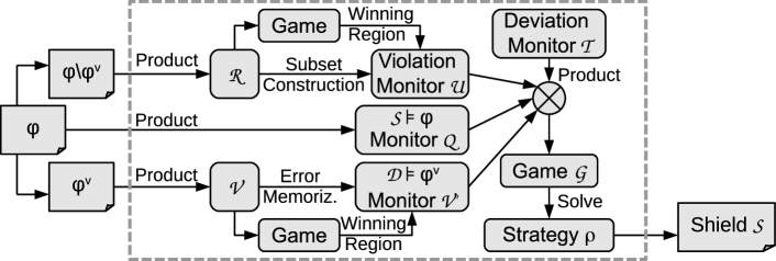
Figure 4: Outline of our $k$-stabilizing generic shield synthesis procedure.

Step 1. Constructing the Violation Monitor $\mathcal{U}$: From $\mathcal{R}$, which represents $\varphi\setminus\varphi^{v}$, we build $\mathcal{U}=(U,u_{0},\Sigma,\delta^{u})$ to monitor property violations by the design. The goal is to identify the latest point in time from which a specification violation can still be corrected with a deviation by the shield. This constitutes the start of the recovery period.

The first phase of this construction (Step 1-a) is to consider the automaton $\mathcal{R}=(R,r_{0},\Sigma,\delta^{r},F^{r})$ as a safety game and compute its winning region $W^{r}\subseteq F^{r}$. The meaning of $W^{r}$ is such that every reactive system $\mathcal{D}\models(\varphi\setminus\varphi^{v})$ must produce outputs in such a way that the next state of $\mathcal{R}$ stays in $W^{r}$. Only when the next state of $\mathcal{R}$ would be outside of $W^{r}$, our shield will be allowed to interfere.

Example 1. Consider the safety automaton $\mathcal{R}$ in Fig. 6, where $i$ is an input, $o$ is an output, and $r_{x}$ is unsafe. The winning region is $W=\{r_{0}\}$ because from $r_{1}$ the input $i$ controls whether $r_{x}$ is visited. The shield must be allowed to deviate from the original transition $r_{0}\rightarrow r_{1}$ if $o\neq i$. In $r_{1}$ it is too late because visiting an unsafe state cannot be avoided any more, given that the shield can modify the value of $o$ but not $i$. ∎

Figure 5: The safety automaton $\mathcal{R}$.

Figure 6: The deviation monitor $\mathcal{T}$.

The second phase (Step 1-b) is to expand the state space from $R$ to $2^{R}$ via a subset construction. The rationale behind it is as follows. If the design makes a mistake (i.e., picks outputs such that $\mathcal{R}$ enters a state $r\not\in W^{r}$ from which the specification cannot be enforced), we have to “guess” what the design actually meant to do in order to find a state from which we can continue monitoring its behavior. We follow a generous approach in order not to treat the design unfairly: we consider all output letters that would have avoided falling out of $W^{r}$, and continue monitoring the design behavior from all the corresponding successor states in parallel. Thus, $\mathcal{U}$ is essentially a subset construction of $\mathcal{R}$, where a state $u\in U$ of $\mathcal{U}$ represents a set of states in $\mathcal{R}$.

The third phase (Step 1-c) is to expand the state space of $\mathcal{U}$ by adding a counter $c\in\{0,\ldots,k\}$ as described in the previous subsection, and adding a special fail-safe state $u_{E}$. The final violation monitor is $\mathcal{U}=(U,u_{0},\Sigma,\delta^{u})$, where $U=(2^{R}\times\{0,\ldots,k\})\cup{u_{E}}$ is the set of states, $u_{0}=(\{r_{0}\},0)$ is the initial state, $\Sigma$ is the set of input letters, and $\delta^{u}$ is the next-state function, which obeys the following rules:

1. $\delta^{u}(u_{E},\sigma)=u_{E}$ (meaning that $u_{E}$ is a trap state),

2. $\delta^{u}((u,c),\sigma)=u_{E}$ if $c>1$ and $\forall r\in u:\delta^{r}(r,\sigma)\not\in W^{r}$,

3. $\delta^{u}((u,c),({\sigma_{I}},{\sigma_{O}}))=(\{r^{\prime}\!\in\!W^{r}\mid\exists r\in u,{\sigma_{O}}^{\prime}\in\Sigma_{O}\operatorname{\mathbin{.}}\delta^{r}(r,({\sigma_{I}},{\sigma_{O}}^{\prime}))=r^{\prime}\},k)$
   if $c\leq 1$ and $\forall r\in u\operatorname{\mathbin{.}}\delta^{r}(r,({\sigma_{I}},{\sigma_{O}}))\not\in W^{r}$, and

4. $\delta^{u}((u,c),\sigma)\!=\!(\{r^{\prime}\!\in\!W^{r}|\exists r\!\in\!u\operatorname{\mathbin{.}}\delta^{r}(r,\sigma)=r^{\prime}\},\textsf{dec}(c))$ if $\exists r\!\in\!u\operatorname{\mathbin{.}}\delta^{r}(r,\sigma)\!\in\!W^{r}$, where $\textsf{dec}(0)=0$ and $\textsf{dec}(c)=c-1$ if $c>0$.

Our construction sets $c=k$ whenever the design leaves the winning region, and not when it enters an unsafe state. Hence, the shield $\mathcal{S}$ can take remedial action as soon as the “the crime is committed”, before the damage is detected, which would have been too late to correct the erroneous outputs of the design.

Example 2. We illustrate the construction of $\mathcal{U}$ using the specification from Fig. 3,

	1g-	1rg	-rr	0gg	0gr	0rg
H	B$\lightning$	B$\lightning$	B	HB$\lightning$	H	HB$\lightning$
B	B$\lightning$	B$\lightning$	B	HFB$\lightning$	H	F
F	B$\lightning$	B$\lightning$	B	FB$\lightning$	FB$\lightning$	F
HB	B$\lightning$	B$\lightning$	B	HFB$\lightning$	H	F
FB	B$\lightning$	B$\lightning$	B	HFB$\lightning$	H	F
HFB	B$\lightning$	B$\lightning$	B	HFB$\lightning$	H	F

Figure 7: $\delta^{u}$ for the spec from Fig. 3.

which is a safety automaton if we make all missing edges point to an (additional) unsafe state. The winning region consists of all safe states, i.e., $W^{r}=\{H,B,F\}$. The resulting violation monitor is $\mathcal{U}=(\{\text{H},\text{B},\text{F},\text{HB},\text{FB},\text{HFB}\}\times\{0,\ldots,k\}\cup u_{E},(\text{H},0),\Sigma,\delta^{u})$, where $\delta^{u}$ is illustrated in Fig. 7 as a table (the graph would be messy), which lists the next state for all possible present states as well as inputs and outputs by the design. Lightning bolts denote specification violations. The update of the counter $c$, which is not included in Fig. 7, is as follows: whenever the design commits a violation (indicated by lightning) and $c\leq 1$, then $c$ is set to $k$. If $c>1$ at the violation, the next state is $u_{E}$. Otherwise, $c$ is decremented. ∎

Step 2. Constructing the Validity Monitor $\mathcal{V^{\prime}}$: From $\mathcal{V}=(V,v_{0},\Sigma,\delta^{v},F^{v})$, which represents $\varphi^{v}$, we build an automaton $\mathcal{V^{\prime}}$ to monitor the validity of $\varphi^{v}$ by solving a safety game on $\mathcal{V}$ and computing the winning region $W^{v}\subseteq F^{v}$. We will use $W^{v}$ to increase the freedom for the shield: since we assume that $\mathcal{D}\models\varphi^{v}$, we are only interested in the cases where $\mathcal{V}$ never leaves $W^{v}$. If it does, our shield is allowed to behave arbitrarily from that point on. We extend the state space from $V$ to $V^{\prime}$ by adding a bit to memorize if we have left the winning region $W^{v}$. Hence, the validity monitor is defined as $\mathcal{V}^{\prime}=(V^{\prime},v_{0}^{\prime},\Sigma,{\delta^{v}}^{\prime},{F^{v}}^{\prime})$, where $V^{\prime}=\mathbb{B}\times V$ is the set of states, $v_{0}^{\prime}=\{\mathsf{false},v_{0}\}$ is the initial state, ${\delta^{v}}^{\prime}((b,v),\sigma)=(b^{\prime},\delta^{v}(v,\sigma))$, where $b^{\prime}=\mathsf{true}$ if $b=\mathsf{true}$ or $\delta^{v}(v,\sigma)\not\in W^{v}$, and $b^{\prime}=\mathsf{false}$ otherwise, and ${F^{v}}^{\prime}=\{(b,v)\in V^{\prime}\mid b=\mathsf{false}\}$.

Step 3. Constructing the Deviation Monitor $\mathcal{T}$: We build $\mathcal{T}=(T,t_{0},\Sigma_{O}\times\Sigma_{O},\delta^{t})$ to monitor the deviation of the shield’s output from the design’s output. Here, $T=\{t_{0},t_{1}\}$ and $\delta^{t}(t,({\sigma_{O}},{\sigma_{O}}^{\prime}))=t_{0}$ iff ${\sigma_{O}}={\sigma_{O}}^{\prime}$. That is, $\mathcal{T}$ will be in $t_{1}$ if there was a deviation in the last time step, and in $t_{0}$ otherwise. This deviation monitor is shown in Fig. 6.

Step 4. Constructing the Safety Game $\mathcal{G}$: Given the monitors $\mathcal{U},\mathcal{V^{\prime}},\mathcal{T}$ and the automaton $\mathcal{Q}$, which represents $\varphi$, we construct a safety game $\mathcal{G}=(G,g_{0},\Sigma_{I}\times\Sigma_{O},\Sigma_{O},$ $\delta^{g},F^{g})$, which is the synchronous product of $\mathcal{U}$, $\mathcal{T}$, $\mathcal{V}^{\prime}$ and $\mathcal{Q}$, such that $G=U\times T\times V^{\prime}\times Q$ is the state space, $g_{0}=(u_{0},t_{0},v_{0}^{\prime},q_{0})$ is the initial state, $\Sigma_{I}\times\Sigma_{O}$ is the input of the shield, $\Sigma_{O}$ is the output of the shield, $\delta^{g}$ is the next-state function, and $F^{g}$ is the set of safe states, such that $\delta^{g}\bigl{(}(u,t,v^{\prime},q),({\sigma_{I}},{\sigma_{O}}),{\sigma_{O}}^{\prime}\bigr{)}=$

$$\bigl{(}\delta^{u}(u,({\sigma_{I}},{\sigma_{O}})),\delta^{t}(t,({\sigma_{O}},{\sigma_{O}}^{\prime})),{\delta^{v}}^{\prime}(v^{\prime},({\sigma_{I}},{\sigma_{O}})),\delta^{q}(q,({\sigma_{I}},{\sigma_{O}}^{\prime}))\bigr{)},$$

and $F^{g}=\{(u,t,v^{\prime},q)\in G\mid v^{\prime}\not\in{F^{v}}^{\prime}\vee((q\in F^{q})\wedge(u=(w,0)\rightarrow t=t_{0}))\}$.

In the definition of $F^{g}$, the term $v^{\prime}\not\in{F^{v}}^{\prime}$ reflects our assumption that $\mathcal{D}\models\varphi^{v}$. If this assumption is violated, then $v^{\prime}\not\in{F^{v}}^{\prime}$ will hold forever, and our shield is allowed to behave arbitrarily. This is exploited by our synthesis algorithm to find a more succinct shield by treating such states as don’t cares. If $v^{\prime}\in{F^{v}}^{\prime}$, we require that $q\in F^{q}$, i.e., it is a safe state in $\mathcal{Q}$, which ensures that the shield output will satisfy $\varphi$. The last term ensures that the shield can only deviate in the $k$-step recovery period, i.e., while $c\neq 0$ in $\mathcal{U}$. If the design makes a second mistake within this period, $\mathcal{U}$ enters $u_{E}$ and arbitrary deviations are allowed. Yet, the shield will still enforce $\varphi$ in this mode (unless $\mathcal{D}\not\models\varphi^{v}$).

Step 5. Solving the Safety Game: We use standard algorithms for safety games (cf. e.g. [15]) to compute a winning strategy $\rho$ for $\mathcal{G}$. Then, we implement this strategy in a new reactive system $\mathcal{S}=(G,g_{0},\Sigma,\Sigma_{O},\delta,\rho)$ with $\delta(g,\sigma)=\delta^{g}(g,\sigma,\rho(g,\sigma))$. $\mathcal{S}$ is the $k$-stabilizing generic shield. If no winning strategy exists, we increase $k$ and try again. In our experiments, we start with $k=1$ and then increase $k$ by 1 at a time.

Theorem 5.1.

Let $\varphi=\{\varphi_{1},\ldots,\varphi_{l}\}$ be a set of critical safety properties $\varphi_{i}=(Q_{i},{q_{0}}_{i},$ $\Sigma,\delta_{i},F_{i})$, and let $\varphi^{v}\subseteq\varphi$ be a subset of valid properties. Let $|V|=\prod_{\varphi_{i}\in\varphi^{v}}|Q_{i}|$ be the cardinality of the product of the state spaces of all properties of $\varphi^{v}$. Similarly, let $|R|=\prod_{\varphi_{i}\not\in\varphi^{v}}|Q_{i}|$. A $k$-stabilizing generic shield with respect to $\varphi\setminus\varphi^{v}$ and $\varphi^{v}$ can be synthesized in $O(k^{2}\cdot 2^{2|R|}\cdot|V|^{4}\cdot|R|^{2})$ time (if one exists).

Proof.

Safety games can be solved in $O(x+y)$ time [15], where $x$ is the number of states and $y$ is the number of edges in the game graph. Our safety game $\mathcal{G}$ has at most $x=((k+1)\cdot 2^{|R|}+1)\cdot(2\cdot|V|)\cdot 2\cdot(|R|\cdot|V|)$ states, so at most $y=x^{2}$ edges. ∎

Variations. The assumption that no second violation occurs within the recovery period increases the chances that a $k$-stabilizing shield exists. However, it can also be dropped with a slight modification of $\mathcal{U}$ in Step 1: if a violation is committed and $c>1$, we set $c$ to $k$ instead of visiting $u_{E}$. This ensures that synthesized shields will handle violations within a recovery period normally. The assumption that the design meant to give one of the allowed outputs if a violation occurs can also be relaxed. Instead of continuing to monitor the behavior from the allowed next states, we can just continue from the set of all states, i.e., traverse to state $(R,k)$ in $\mathcal{U}$. The assumption that $\mathcal{D}\models\varphi^{v}$, i.e., the design satisfies some properties, is also optional. By removing $\mathcal{V}$ and $\mathcal{V}^{\prime}$, the construction can be simplified at the cost of less implementation freedom for the shield.

By solving a Büchi game (which is potentially more expensive) instead of a safety game, we can also eliminate the need to increase $k$ iteratively until a solution is found. This is outlined in Appendix 0.A.

6 Experiments

We have implemented the $k$-stabilizing shield synthesis procedure in a proof-of-concept tool. Our tool takes as input a set of safety properties, defined as automata in a simple textual representation. The product of these automata, as well as the subset construction in Step 1 of our procedure is done on an explicit representation. The remaining steps are performed symbolically using Binary Decision Diagrams (BDDs). Synthesis starts with $k=1$ and increments $k$ in case of unrealizability until a user-defined bound is hit. Our tool is written in Python and uses CUDD [1] as the BDD library. Our tool can output shields in Verilog and SMV. It can also use the model checker VIS [6] to verify that the synthesized shield is correct.

We have conducted three sets of experiments, where the benchmarks are (1) selected properties for a traffic light controller from the VIS [6] manual, (2) selected properties for an ARM AMBA bus arbiter [4], and (3) selected properties from LTL specification patterns [11]. None of these examples makes use of $\varphi^{v}$, i.e., $\varphi^{v}$ is always empty. The source code of our proof-of-concept synthesis tool as well as the input files and instructions to reproduce our experiments are available for download.

Traffic Light Controller Example. We used the safety specification in Fig. 3 as input,

Figure 8: Traffic light shield.

for which our tool generated a $1$-stabilizing shield within a fraction of a second. The shield has 6 latches and 95 (2-input) multiplexers, which is then reduced by ABC [7] to 5 latches and 41 (2-input) AIG gates. However, most of the states are either unreachable or equivalent. The behavior of the shield is illustrated in Fig. 8. Edges are labeled with the inputs of the shield. Red dashed edges denote situations where the output of the shield is different from its inputs. The modified output is written after the arrow. For all non-dashed edges, the input is just copied to the output. Clearly, the states X, Y, and Z correspond to H, B, and F in Fig. 3.

We also tested the synthesized shield using the traffic light controller of [16], which also appeared in the user manual of VIS [6]. This controller has one input (car) from a car sensor on the farm road, and uses a timer to control the length of the different phases. We set the “short” timer period to one tick and the “long” period to two ticks.

Figure 9: Traffic light implementation.

The resulting behavior without preemption is visualized in Fig. 9, where nodes are labeled with names and outputs, and edges are labeled with conditions on the inputs. The red dashed arrow represents a subtle bug we introduced: if the last car on the farm road exits the crossing at a rare point in time, then the controller switches from rg to gr without passing rr. This bug only shows up in very special situations, so it can go unnoticed easily. Preemption is implemented by modifying both directions to r without changing the state if $\textsf{p}=1$. We introduced another bug here as well: only the highway is switched to r if $\textsf{p}=1$, whereas the farm road is not. This bug can easily go unnoticed as well, because the farm road is mostly red anyway. The following trace illustrates how the synthesized shield handles these errors:

Step

0

1

2

3

4

5

6

7

8

9

10

11

12

13

14

15

State in Fig. 3 (safety spec.)

H

H

B

H

B

B

F

F

F,B

H

H

B

B

B

B

…

State in Fig. 9 (buggy design)

S0

S1

S2

S3

S4

S5

S6

S0

S1

S2

S3

S4

S5

S8

S9

…

State in Fig. 8 (shield)

X

X

Y

X

Y

Y

Z

Z

Y

X

X

Y

Y

Y

Y

…

Input (p,car)

00

11

01

01

01

01

00

00

00

01

01

00

10

00

00

…

Design output

gr

rr

gr

rr

rr

rg

rg

gr$\lightning$

gr

gr

rr

rr

rg$\lightning$

rr

rr

…

Shield output

gr

rr

gr

rr

rr

rg

rg

rr

gr

gr

rr

rr

rr

rr

rr

…

The first bug strikes at Step 7. The shield corrects it with output rr. A $2$-stabilizing shield could also have chosen rg, but this would have made a second deviation necessary in the next step. Our shield is $1$-stabilizing, i.e., it deviates only at the step of the violation. After this correction, the shield continues monitoring the design from both state F and state B of Fig. 3, as explained earlier, to detect future errors. Yet, this uncertainty is resolved in the next step. The second bug in Step 12 is simpler: outputting rr is the only way to correct it, and the next state in Fig. 3 must be B.

When only considering the properties 1 and 2 from Section 2, the synthesized shield has no latches and three AIG gates after optimization with ABC [7].

ARM AMBA Bus Arbiter Example. We used properties of an ARM AMBA bus arbiter [4] as input to our shield synthesis tool. Due to page limit, we only present the result on one example property, and then present the performance results for other properties. The property that we enforced was Guarantee 3 from the specification of [4], which says that if a length-four locked burst access starts, no other access can start until the end of this burst. The safety automaton is shown in Fig. 11, where B, s and R are short for $\texttt{hmastlock}\wedge\texttt{HBURST=BURST4}$, start, and HREADY, respectively. Lower case signal names are outputs, and upper-cases are inputs of the arbiter. S_x is unsafe. S0 is the idle state waiting for a burst to start ($\texttt{B}\wedge\texttt{s}$). The burst is over if input R has been $\mathsf{true}$ $4$ times. State S$i$, where $i=1,2,3,4$, means that R must be $\mathsf{true}$ for $i$ more times. The counting includes the time step where the burst starts, i.e., where S0 is left. Outside of S0, s is required to be $\mathsf{false}$.

Figure 10: Guarantee 3 from [4].

Step	3	4	5	6	7	8	9	10	11	12
State in Fig. 11	S0	S4	S3	S2	S1	S0	S0	S0	S0	…
State in Design	S0	S3	S2	S1	S0	S3	S2	S1	S0	…
B	1	1	1	1	1	1	1	1	1	…
R	0	1	1	1	1	1	1	1	1	…
s from Design	1	0	0	0	1$\lightning$	0	0	0	0	…
s from Shield	1	0	0	0	0	0	0	0	0	…

Figure 11: Shield execution results.

Our tool generated a 1-stabilizing shield within a fraction of a second. The shield has 8 latches and 142 (2-input) multiplexers, which is then reduced by ABC [7] to 4 latches and 77 AIG gates. We verified it against an arbiter implementation for 2 bus masters, where we introduced the following bug: the design does not check R when the burst starts, but behaves as if R was $\mathsf{true}$. This corresponds to removing the transition from S0 to S4 in Fig. 11, and going to S3 instead. An execution trace is shown in Fig. 11. The first burst starts with $\texttt{s}=\mathsf{true}$ in Step 3. R is $\mathsf{false}$, so the design counts wrongly. The erroneous output shows up in Step 7, where the design starts the next burst, which is forbidden, and thus blocked by the shield. The design now thinks that it has started a burst, so it keeps $\texttt{s}=\mathsf{false}$ until R is $\mathsf{true}$ 4 times. Actually, this burst start has been blocked by the shield, so the shield waits in S0. Only after the suppressed burst is over, the components are in sync again, and the next burst can start normally.

Table 1: Performance for AMBA [4].

Property	$|Q|$	$|I|$	$|O|$	$k$	Time [sec]
G1	3	1	1	1	0.1
G1+2	5	3	3	1	0.1
G1+2+3	12	3	3	1	0.1
G1+2+4	8	3	6	2	7.8
G1+3+4	15	3	5	2	65
G2+3+4	17	3	6	?	$>$3600
G1+2+3+5	18	3	4	2	242
G1+2+4+5	12	3	7	?	$>$3600
G1+3+4+5	23	3	6	?	$>$3600

To evaluate the performance of our tool, we ran a stress test with increasingly larger sets of safety properties for the ARM AMBA bus arbiter in [4]. Table 1 summarizes the results. The columns list the number of states, inputs, and outputs, the minimum $k$ for which a $k$-stabilizing shield exists, and the synthesis time in seconds. All experiments were performed on a machine with an Intel i5-3320M CPU@2.6 GHz, 8 GB RAM, and a 64-bit Linux. Time-outs (G2+3+4, G1+2+4+5 and G1+3+4+5) occurred only when the number of states and input/output signals grew large. However, this should not be a concern in practice because the set of critical properties of a system is usually much smaller, e.g., often consisting of invariance properties with a single state.

Table 2: Synthesis results for the LTL patterns [11].

Nr.	Property	$b$	$|Q|$	Time	#Lat-	#AIG-
				[sec]	ches	Gates
1	$\operatorname{\mathsf{G}}\neg p$	-	2	0.01	0	0
2	$\operatorname{\mathsf{F}}r\rightarrow(\neg p\mathbin{\mathsf{U}}r)$	-	4	0.34	2	6
3	$\operatorname{\mathsf{G}}(q\rightarrow\operatorname{\mathsf{G}}(\neg p))$	-	3	0.34	2	6
4	$\operatorname{\mathsf{G}}((q\wedge\neg r\wedge\operatorname{\mathsf{F}}r)\rightarrow(\neg p\mathbin{\mathsf{U}}r))$	-	4	0.34	1	9
5	$\operatorname{\mathsf{G}}(q\wedge\neg r\rightarrow(\neg p\mathbin{\mathsf{W}}r))$	-	3	0.01	2	14
6	$\operatorname{\mathsf{F}}p$	0	3	0.34	1	1
6	$\operatorname{\mathsf{F}}p$	256	259	33	18	134
7	$\neg r\mathbin{\mathsf{W}}(p\wedge\neg r)$	-	3	0.05	3	11
8	$\operatorname{\mathsf{G}}(\neg q)\vee\operatorname{\mathsf{F}}(q\wedge\operatorname{\mathsf{F}}p)$	0	3	0.04	3	11
8	$\operatorname{\mathsf{G}}(\neg q)\vee\operatorname{\mathsf{F}}(q\wedge\operatorname{\mathsf{F}}p)$	4	7	0.04	6	79
8	$\operatorname{\mathsf{G}}(\neg q)\vee\operatorname{\mathsf{F}}(q\wedge\operatorname{\mathsf{F}}p)$	16	19	0.03	10	162
8	$\operatorname{\mathsf{G}}(\neg q)\vee\operatorname{\mathsf{F}}(q\wedge\operatorname{\mathsf{F}}p)$	64	67	0.37	14	349
8	$\operatorname{\mathsf{G}}(\neg q)\vee\operatorname{\mathsf{F}}(q\wedge\operatorname{\mathsf{F}}p)$	256	259	34	18	890
9	$\operatorname{\mathsf{G}}(q\wedge\neg r\rightarrow(\neg r\mathbin{\mathsf{W}}(p\wedge\neg r)))$	-	3	0.05	2	12
10	$\operatorname{\mathsf{G}}(q\wedge\neg r\rightarrow(\neg r\mathbin{\mathsf{U}}(p\wedge\neg r)))$	12	14	5.4	14	2901
10	$\operatorname{\mathsf{G}}(q\wedge\neg r\rightarrow(\neg r\mathbin{\mathsf{U}}(p\wedge\neg r)))$	14	16	38	15	6020
10	$\operatorname{\mathsf{G}}(q\wedge\neg r\rightarrow(\neg r\mathbin{\mathsf{U}}(p\wedge\neg r)))$	16	18	377	18	13140

LTL Specification Patterns. Dwyer et al. [11] studied the frequently used LTL specification patterns in verification. As an exercise, we applied our tool to the first 10 properties from their list [2] and summarized the results in Table 2. For a property containing liveness aspects (e.g., something must happen eventually), we imposed a bound on the reaction time to obtain the safety (bounded-liveness) property. The bound on the reaction time is shown in Column 3. The last four columns list the number of states in the safety specification, the synthesis time in seconds, and the shield size (latches and AIG gates). Overall, our method runs sufficiently fast on all properties and the resulting shield size is small. We also investigated how the synthesis time increased with an increasingly larger bound $b$. For Property 8 and Property 6, the run time and shield size remained small even for large automata. For Property 10, the run time and shield size grew faster, indicating room for further improvement. As a proof-of-concept implementation, our tool has not yet been optimized specifically for speed or shield size – we leave such optimizations for future work.

7 Conclusions

We have formally defined the shield synthesis problem for reactive systems and presented a general framework for solving the problem. We have also implemented a new synthesis procedure that solves a concrete instance of this problem, namely the synthesis of $k$-stabilizing generic shields. We have evaluated our new method on two hardware benchmarks and a set of LTL specification patterns. We believe that our work points to an exciting new direction for applying synthesis, because the set of critical properties of a complex system tends to be small and relatively easy to specify, thereby making shield synthesis scalable and usable. Many interesting extensions and variants remain to be explored, both theoretically and experimentally, in the future.

Appendix 0.A Synthesis of Stabilizing Generic Shields

In this section, we present a method for synthesizing $k$-stabilizing shields with arbitrary but finite $k$. We call such shields stabilizing (without the “$k$”). A synthesis procedure for stabilizing shields is also useful as a preprocessing step if we want to enforce a particular (or minimal) $k$: Even for a realizable specification, the $k$-stabilizing shield synthesis problem may be unrealizable for any finite $k$. When specification $\varphi$ is realizable, there exists a reactive system $\mathcal{D}^{\prime}$ such that $\mathcal{D}^{\prime}\models\varphi$. However, it does not mean that a shield $\mathcal{S}$ exists for any design $\mathcal{D}$, such that $(\mathcal{D}\circ\mathcal{S})\models\varphi$, and $(\mathcal{D}\circ\mathcal{S})$ deviates from $\mathcal{D}$ for at most $k$ time steps.

Example 3. Consider the safety specification on the right, where $o_{1}$ and $o_{2}$ are

outputs, and $r_{x}$ is unsafe. The design must produce either $o_{1}\wedge\neg o_{2}$ globally or $\neg o_{1}$ globally. The $k$-stabilizing shield synthesis problem is unrealizable for any finite $k$: if the design produces $o_{1}\wedge o_{2}$ initially, the shield must deviate to either $o_{1}\wedge\neg o_{2}$ or $\neg o_{2}$. In the former case, the design could produce $\neg o_{1}$ from that point on, in the latter case $o_{1}\wedge\neg o_{2}$. This would cause an indefinite deviation with only a single violation. ∎

Whether a $k$-stabilizing shield exists for some finite $k$ is difficult to detect with the synthesis procedure from Section 5.2. In case of unrealizability of the shield for a given $k$, we cannot know if we just need to increase $k$, or if no finite $k$ would work. The synthesis process presented in the following sub-section will decide the realizability problem. We can also synthesize a stabilizing shield, measure its $k$, and minimize this $k$ further with the procedure from Section 5.2 until we hit the unrealizability barrier.

0.A.1 Construction for Synthesizing Stabilizing Shields

A generic stabilizing shield can be synthesized (if one exists) with only a few modifications to the procedure from Section 5.2. Instead of a counter $c\in\{0,\ldots,k\}$, we use a counter $d\in\{0,1,2\}$ with only three different values. Intuitively, $d=2$ is an abstraction for $c>1$. We construct a Büchi game that is won if $d\leq 1$ infinitely often (and all the other shield requirements are satisfied). A Büchi game is like a safety game, but the given set of final states must be visited infinitely often for the system to win the game. A winning strategy for this Büchi game corresponds to a $k$-stabilizing shield with some finite $k$, and the $k$ can even be computed during synthesis. The construction is similar to Section 5.2, with only a few modifications:

Step 1. Instead of using a counter $c\in\{0,\ldots,k\}$, we use a three-valued counter $d\in\{0,1,2\}$ to track whether we are currently in the recovery phase or not. Intuitively, $d=2$ if $c$ would be $>1$. That is, $d$ is $0$ initially. If $d<2$ and the design makes a mistake (leaves $W^{r}$), then $d$ is set to $2$. If it was already $2$, we enter $u_{E}$. In order to decide when to decrement $d$ from $2$ to $1$, we add a special output $r$ to the shield. If this output is set to $\mathsf{true}$ and $d=2$, then $d$ is set to $1$ in the next step. The behavior for $d=1$ is the same as in Section 5.2: if another violation occurs, $d$ is set to $2$. Otherwise, $d$ is decremented to $1$. We denote this slightly modified violation monitor by $\mathcal{U}^{\prime}=(U^{\prime},u_{0}^{\prime},\Sigma\times 2^{\{r\}},{\delta^{u}}^{\prime})$ with $U^{\prime}=(2^{R}\times\{0,1,2\})\cup{u_{E}}$. The subsequent steps will ensure that the shield will only be allowed to deviate if $d>0$ in the next step. We will also require that $d$ cannot be $2$ indefinitely.

Step 2 and Step 3 are performed as described in Section 5.2.

Step 4. We construct a Büchi game $\mathcal{G}^{\prime}=(G^{\prime},g_{0}^{\prime},\Sigma_{I}\times\Sigma_{O},\Sigma_{O}\times 2^{\{r\}},{\delta^{g}}^{\prime},{F^{g}}^{\prime})$ as the synchronous product of $\mathcal{U}^{\prime}$, $\mathcal{T}$, $\mathcal{V}^{\prime}$ and $\mathcal{Q}$ as follows:

• $G^{\prime}=U^{\prime}\times T\times V^{\prime}\times Q\times\mathbb{B}\times\mathbb{B}$,

• $g_{0}^{\prime}=(u_{0}^{\prime},t_{0},v_{0}^{\prime},q_{0},\mathsf{false},\mathsf{false})$,

• ${\delta^{g}}^{\prime}\bigl{(}(u^{\prime},t,v^{\prime},q,m,n),({\sigma_{I}},{\sigma_{O}}),({\sigma_{O}}^{\prime},r)\bigr{)}=\bigl{(}{\delta^{u}}^{\prime}(u^{\prime},(({\sigma_{I}},{\sigma_{O}}),r)),\\ \delta^{t}(t,({\sigma_{O}},{\sigma_{O}}^{\prime})),{\delta^{v}}^{\prime}(v^{\prime},({\sigma_{I}},{\sigma_{O}})),\delta^{q}(q,({\sigma_{I}},{\sigma_{O}}^{\prime})),m^{\prime},n^{\prime}\bigr{)}$, where

  • $m^{\prime}=\mathsf{true}$ iff $m=\mathsf{true}$ or $q\not\in F^{q}$

  • $n^{\prime}=\mathsf{true}$ iff $n=\mathsf{true}$ or $u^{\prime}=(w,0)\wedge t=t_{1}$, and

• ${F^{g}}^{\prime}=\{(u^{\prime},t,v^{\prime},q,m,n)\in G^{\prime}\mid v^{\prime}\not\in{F^{v}}^{\prime}\vee(\neg n\wedge\neg m\wedge d\leq 1)\}$.

The intuition behind this construction is as follows. We extend the state space of the synchronous product by two bits, $m$ and $n$. The bit $m$ is $\mathsf{true}$ if the execution has ever visited an unsafe state in $\mathcal{Q}$. The bit $n$ is $\mathsf{true}$ if there has been an illegal deviation. With this information, the accepting states (that need to be visited infinitely often) are then defined as follows. Outside of ${F^{v}}^{\prime}$, everything is accepting. This makes sure that the shield can behave arbitrarily if $\mathcal{D}\not\models\varphi^{v}$. Otherwise, a state is accepting if $d\leq 1$ (the last recovery period is over), $m$ is $\mathsf{false}$ ($\mathcal{D}\circ\mathcal{S}\models\varphi$ so far) and $n$ is $\mathsf{false}$ (no illegal deviations so far). Visiting ${F^{g}}^{\prime}$ infinitely often implies that recovery periods are over infinitely often, and $m$ and $n$ are never $\mathsf{true}$ (these bits cannot change back to $\mathsf{false}$).

Step 5. Just like safety games, Büchi games also have a memoryless strategy. We compute such a strategy and implement it as described in Section 5.2. If no such strategy exists (which is easy to detect during synthesis), then this is reported to the user.

Discussion. Note that the Büchi objective ensures that recovery phases are over infinitely often, but not that they are bounded in time. There may exist a strategy to satisfy the Büchi objective without any finite bound on the recovery time. E.g., the first recovery phase could take 2 steps, the second one 4 steps, the third one 8 steps, etc. However, such a strategy would require infinite memory. We construct and implement a memoryless strategy, which guarantees a bounded recovery. We can even measure the maximum length of any recovery phase while synthesizing the shield: Büchi games can be solved with a doubly-nested fixpoint computation [15]. The number of iterations of the inner fixpoint (in the last iteration of the outer fixpoint) corresponds to the maximum number of steps needed to reach a state of ${F^{g}}^{\prime}$, i.e., a state where the recovery is over. Hence, this value is also the maximum length of a recovery period, i.e., the value $k$ for the resulting $k$-stabilizing shield.

References

- [1] CUDD: CU Decision Diagram Package. ftp://vlsi.colorado.edu/pub/.
- [2] LTL Specification Patterns. http://patterns.projects.cis.ksu.edu/documentation/patterns/ltl.shtml.
- [3] R. Bloem, K. Chatterjee, K. Greimel, T. Henzinger, G. Hofferek, B. Jobstmann, B. Könighofer, and R. Könighofer. Synthesizing robust systems. Acta Inf., 51:193–220, 2014.
- [4] R. Bloem, B. Jobstmann, N. Piterman, A. Pnueli, and Y. Sa’ar. Synthesis of reactive(1) designs. J. Comput. Syst. Sci., 78(3):911–938, 2012.
- [5] R. Bloem, B. Könighofer, R. Könighofer, and C. Wang. Shield synthesis: Runtime enforcement for reactive systems. In TACAS. Springer, 2015. To appear.
- [6] R. K. Brayton et al. VIS: A system for verification and synthesis. In CAV, LNCS 1102, pages 428–432. Springer, 1996.
- [7] R. K. Brayton and A. Mishchenko. ABC: An academic industrial-strength verification tool. In CAV, LNCS 6174, pages 24–40. Springer, 2010.
- [8] J. R. Büchi and L. H. Landweber. Solving sequential conditions by finite-state strategies. Trans. Amer. Math. Soc. 138, pages 367–378, 1969.
- [9] A. Church. Logic, arithmetic, and automata. Int. Congr. Math. 1962, pages 23–35, 1963.
- [10] E. M. Clarke and E. A. Emerson. Design and synthesis of synchronization skeletons using branching time temporal logic. In Logics of Programs, LNCS 131, pages 52–71, 1981.
- [11] M. B. Dwyer, G. S. Avrunin, and J. C. Corbett. Patterns in property specifications for finite-state verification. In ICSE, pages 411–420. ACM, 1999.
- [12] R. Ehlers and U. Topcu. Resilience to intermittent assumption violations in reactive synthesis. In HSCC, pages 203–212. ACM, 2014.
- [13] Y. Falcone, J.-C. Fernandez, and L. Mounier. What can you verify and enforce at runtime? STTT, 14(3):349–382, 2012.
- [14] J. Ligatti, L. Bauer, and D. Walker. Run-time enforcement of nonsafety policies. ACM Trans. Inf. Syst. Secur., 12(3), 2009.
- [15] R. Mazala. Infinite games. In Automata, Logics, and Infinite Games: A Guide to Current Research, LNCS 2500, pages 23–42. Springer, 2001.
- [16] C. Mead and L. Conway. Introduction to VLSI systems. Addison-Wesley, 1980.
- [17] A. Pnueli and R. Rosner. On the synthesis of a reactive module. In POPL, pages 179–190. ACM, 1989.
- [18] J. P. Quielle and J. Sifakis. Specification and verification of concurrent systems in CESAR. In Symposium on Programming, LNCS 137. Springer, 1982.
- [19] M. O. Rabin. Automata on Infinite Objects and Church’s Problem. Regional Conference Series in Mathematics. American Mathematical Society, 1972.
- [20] F. B. Schneider. Enforceable security policies. ACM Trans. Inf. Syst. Secur., 3:30–50, 2000.