The gravitational-wave signal generated by a galactic population of double neutron-star binaries
Abstract
We investigate the gravitational wave (GW) signal generated by a population of double neutron-star binaries (DNS) with eccentric orbits caused by kicks during supernova collapse and binary evolution. The DNS population of a standard Milky-Way type galaxy has been studied as a function of star formation history, initial mass function (IMF) and metallicity and of the binary-star common-envelope ejection process. The model provides birth rates, merger rates and total numbers of DNS as a function of time. The GW signal produced by this population has been computed and expressed in terms of a hypothetical space GW detector (eLISA) by calculating the number of discrete GW signals at different confidence levels, where ‘signal’ refers to detectable GW strain in a given frequency-resolution element. In terms of the parameter space explored, the number of DNS-originating GW signals is greatest in regions of recent star formation, and is significantly increased if metallicity is reduced from 0.02 to 0.001, consistent with Belczynski et al. (2010). Increasing the IMF power-law index (from –2.5 to –1.5) increases the number of GW signals by a large factor. This number is also much higher for models where the common-envelope ejection is treated using the mechanism (energy conservation) than when using the mechanism (angular-momentum conservation). We have estimated the total number of detectable DNS GW signals from the Galaxy by combining contributions from thin disc, thick disc, bulge and halo. The most probable numbers for an eLISA-type experiment are 01600 signals per year at S/N1, 0900 signals per year at S/N3, and 0570 at S/N5, coming from about 065, 060 and 050 resolved DNS respectively.
keywords:
Gravitational waves - neutron stars - Stars: binaries: close - Galaxy: structure - Galaxy: stellar content1 Introduction
Most stars are members of binary or multiple star systems. Over 70% of massive stars (O-type stars) have a nearby companion which will affect their evolution, with over one half doing so before they leave the main sequence (MS) (Sana et al., 2012; Langer, 2012). If both members of a binary are massive enough to end their evolution as core-collapse supernovae111Neutron stars can also be formed by accretion of Oxygen-Neon white dwarfs, after one or two explosions, the final product could become a double neutron-star binary (DNS), a neutron-star plus black-hole binary, or a double black-hole binary. Evidence that such systems do form is provided by the double pulsar PSR J0737-3039A/B (Burgay et al., 2003; Lyne et al., 2004; Kramer & Stairs, 2008). Such compact binaries are expected to be a significant source of gravitational wave (GW) radiation (Barish & Weiss, 1999; Ricci & Brillet, 1997; Postnov & Yungelson, 2006). They are amongst the sources most likely to be detected by a gravitational wave detector in the frequency range Hz. Aasi et al. (2014) measured upper limits of the GW strain amplitudes from hundreds of pulsars using data from recent runs of the ground-based GW observatories - LIGO, Virgo and GEO600, and showed that there are good prospects for detections in the 10 - 1000 Hz range with the advanced LIGO and Virgo detectors.
Double neutron-star and black-hole binaries play an important role in testing the theory of General Relativity, whilst double pulsars provide probes of magnetospheric physics. The accurate timing of pulsars orbiting a black hole can be used to constrain the strain amplitude of gravitational waves and the physical properties of the black hole. (Kramer et al., 2004).
| DNS | |||||
|---|---|---|---|---|---|
| PSR | (d) | Hz | |||
| J0737–3039 | 0.102 | 0.09 | Yes | 7.9 | |
| J1906+0746 | 0.17 | 0.09 | Yes | 8.5 | |
| B1913+16 | 0.3 | 0.62 | Yes | 8.5 | |
| B2127+11C | 0.3 | 0.68 | Yes | 8.3 | |
| J1756–2251 | 0.32 | 0.18 | Yes | 10.2 | |
| B1534+12 | 0.4 | 0.27 | Yes | 9.4 | |
| J1829+2456 | 1.18 | 0.14 | No | 10.8 | |
| J1518+4904 | 8.6 | 0.25 | No | 12.4 | |
| J1811–1736 | 18.8 | 0.83 | Yes | 13.0 | |
| B1820–11 | 357.8 | 0.79 | No | 15.8 |
In order of discovery: PSR B1913+16: Hulse & Taylor (1975), PSR B1820–11: Lyne & McKenna (1989), PSR B1534+12: Wolszczan (1991), PSR B2127+11C: Prince et al. (1991), PSR J1518+4904: Nice et al. (1996), PSR J1811–1736: Lyne et al. (2000), PSR J0737–3039A/B: Burgay et al. (2003); Lyne et al. (2004), PSR J1829+2456: Champion et al. (2004), PSR J1756–2251: Faulkner et al. (2005), and PSR J1906+0746: Lorimer et al. (2006).
At present (2014) 7 DNSs, have been confirmed and 3 more are suspected (Table 1). Of these, half have merger timescales shorter than a Hubble time. Half also show eccentric orbits, even at relatively short periods. Bayesian statistical analyses based on these observations indicate that an optimistic Galactic DNS merger rate may be up to yr-1, implying that their number should be approximately a few million (Kalogera et al., 2001, 2004) if we assume the age of the Galaxy is Gyr. This number is roughly 1-2 orders of magnitude higher than estimated from binary star population synthesis (Nelemans et al., 2001; Osłowski et al., 2011; Dominik et al., 2012), although the uncertainty in the Bayesian analysis can exceed one order of magnitude.
Theoretical investigations of the GW signal from Galactic DNSs have been carried out by (e.g.) Allen et al. (1999); Belczynski et al. (2010a); Rosado (2011); Allen et al. (2012). The stochastic GW background produced by DNS mergers in low-redshift galaxies (up to z5) has been investigated by Regimbau & de Freitas Pacheco (2006) (also see Rosado (2011)), who found that the signal should be detectable by the new generation of ground-based interferometers. Zhu et al. (2013) studied the GW background from compact binary mergers, and showed that, below 100 Hz, the background depends primarily on the local merger rate and the average chirp mass and is independent of the chirp mass distribution. In addition, the effects of cosmic star formation rates and delay times between the formation and merger of binaries are linear below 100 Hz in their model. Belczynski et al. (2010a) studied the GW background and foreground signal from a Galactic population of double compact objects using the binary-star population-synthesis (BSPS) method. They concluded that only a few (2-4) NS-NS binaries in the Galaxy would have been detectable by the cancelled space observatory LISA. However, approximations for (i) the calculation of the GW signal from individual DNS binaries, and (ii) the employment of crucial initial conditions and the treatment of important physical processes in the BSPS method, may result in quite large uncertainties.
In order to understand the signal detected by sufficiently sensitive GW detectors, it is necessary to characterize the radiation from all GW-emitting populations, including DNS. This paper presents a study of the GW signal from the Galactic population of steady-state DNSs222 A DNS merger would be clearly indicated by a strong GW signal at rapidly rising frequencies Hz. The most optimistic Galactic DNS merger rates are – see § 3. as a function of several key parameters, including the Galactic star-formation history, the initial-mass function, metallicity, and the physics of common-envelope evolution. It examines how this DNS population differs from the Galactic double-white-dwarf (DWD) population, and establishes a basis for computing the GW signal due to extragalactic DNS populations. We describe the methods used to model the DNS population in the Galactic disc, the emission and superposition of GW signals, and the reduction of the data in terms of a conceptual GW experiment (eLISA) in § 2. Major results are presented in § 3. Implications, observations and previous work are discussed in § 4. The main conclusions are reviewed in § 5.
2 Methods
2.1 Binary-star population synthesis
In this section, we review the important physical processes in binary star evolution and the initial and boundary conditions for population synthesis to obtain a sample of double compact objects. Population synthesis, including individual stellar-evolution tracks and initial conditions, was carried out using the method described by Yu & Jeffery (2010, 2011) and Hurley et al. (2000, 2002) in an initial study of the present Galactic double degenerates population. Note that we take some standard parameters for the Galactic disc (or the Galaxy) to represent a Milky-way type galaxy.
2.1.1 Common-envelope evolution
When one star in a binary fills its Roche lobe either by evolutionary expansion or by orbital shrinkage, Roche lobe overflow (RLOF) occurs. The Roche radius of the primary is given by
| (1) |
where is more generally the semimajor axis of the orbit and is the mass ratio of primary and secondary (Eggleton, 1983). Hurley et al. (2000, 2002) have shown that there is a critical mass ratio of a binary star which can be used to distinguish the stable RLOF and common envelope (CE) phases, where is a function of primary mass , its core mass , and the mass-transfer efficiency of the donor. We adopt
| (2) |
where = 0.3 is the exponent of the mass-radius relation at constant luminosity for giant stars (Hurley et al., 2000, 2002).
The calculation of the orbital parameters (e.g. orbital separation) of a binary after CE ejection in our model is based on one of two assumptions: either 1) angular momentum conservation (mechanism) or 2) energy conservation (mechanism).
In the first case, we consider the angular momentum lost by a binary system undergoing non-conservative mass transfer to be described by the decrease of primary mass times a factor (Paczyński & Ziółkowski, 1967; Nelemans et al., 2000):
| (3) |
where is the orbital angular momentum of the pre-mass transfer binary; is the final orbital angular momentum after CE ejection; and is the primary mass and its core mass respectively; is the secondary mass.
Combining the above equation with the fraction of angular momentum lost during the mass transfer, , and Kepler’s law, we have the ratio of final to initial orbital separation
| (4) |
where and are the orbital separations before and after the CE phase; is the sum of the primary and secondary mass before the CE phase. Nelemans & Tout (2005) investigated the mass-transfer phase of the progenitors of white dwarfs in binaries employing the -mechanism based on 10 observed systems and deduced a value of in the range of 1.4 – 1.7. In order to investigate the influence of angular momentum loss on the rates of DCOs, we here adopt 1.3 and 1.5.
In the second case, CE ejection of a binary star requires that the envelope binding energy, including gravitational-binding and recombination energies, must represent a significant fraction of the orbital energy (Webbink, 1984).
| (5) |
where is a structure parameter depending on the evolutionary state of the donor, is the CE ejection efficiency representing how much orbital energy was used to eject the CE, is the Roche lobe radius of the donor at the onset of mass transfer, and is the gravitational constant (Webbink, 1984). Rearranging in the form of Eq.4, we have
| (6) |
In this paper, we adopt = 1.0, and = 0.5 and 1.0.
A major difference between the two CE ejection formulations is that energy conservation implies a significant spiral-in stage in order to eject the envelope (if we only consider the orbital energy as the main engine) whilst the mechanism does not, implying that the orbital separation can be larger after CE ejection in the latter case. In particular, under the assumption of no external moment imposed on a conservative mass-transfer binary, the angular momentum of the binary must be conservative, and the final orbital separation can be written as
| (7) |
where is the fraction of mass transferred from the primary to the secondary. This means that in conservative evolution, if prior to mass transfer, the orbital separation incfreases after mass transfer.
Although both CE ejection formulations can reproduce observations (Nelemans & Tout, 2005; Webbink, 2008) via a variation of free parameters, considering both conservation laws may be a better approach to constrain the CE evolution and final orbit of a binary. Note that in this paper we neglect viscosity, friction between the CE and the stellar cores, and the potential nuclear and chemical energy in the system.
2.1.2 Gravitational radiation, magnetic braking, and tidal interaction
Other mechanisms which reduce the orbital separation of a binary system include gravitational radiation and magnetic braking. A close compact binary system driven by gravitational radiation may eventually undergo a mass transfer phase, ultimately leading to coalescence. Using the average energy () and angular momentum () loss during one orbital period, we deduce the decay of orbital separation and eccentricity with respect to time to be
| (8) |
| (9) |
This calculation is consistent with our calculation of the GW signal from DNS described in § 2.2.
Gravitational radiation could explain the formation of cataclysmic variables (CVs) with orbital periods less than 3h, while magnetic braking of the tidally coupled primary by its own magnetic wind would account for orbital angular-momentum loss from CVs with periods up to 10 h (Faulkner, 1971; Zangrilli et al., 1997). We use the formula for the rate of angular-momentum loss due to magnetic braking derived by Rappaport et al. (1983) and Skumanich (1972):
| (10) |
where , and are the radius, envelope mass and mass of a star with a convective envelope, and is the spin angular velocity of the star.
Tidal interaction caused by the gravity differential plays an important role in the synchronization of stellar rotation and orbital motion, and the circularization of the orbit. Relatively complete descriptions of the tidal evolution have been given by Hurley et al. (2002) and Belczynski et al. (2008). In this paper, we adopt the same formulae and procedures to deal with the tidal evolution as by Hut (1981); Zahn (1977); Campbell (1984); Rasio et al. (1996) and Hurley et al. (2002).
2.1.3 Formation of double neutron stars
Our simulations assume three routes for the formation of neutron stars: i) if a star has core mass of at shell helium ignition, it evolve through double-shell thermal-pulses up the asymptotic giant branch. The star may become a neutron star if its core mass grows and eventually exceeds ; ii) if the core mass of the star on the thermal-pulsing asymptotic giant branch does not exceed but it is heavy enough () to become an electron-degenerate oxygen-neon white dwarf which may become a neutron star via accretion-induced collapse; iii) if a star has a core mass of at the start of the early asymptotic giant (or red giant) branch, it will become a neutron star without ascending the thermal-pulsing asymptotic giant branch. If the core mass of a star at the time of supernova explosion is sufficiently high (), it will most likely become a black hole unless significant mass loss takes place. These criteria are consistent with Hurley et al. (2000).
The gravitational mass of neutron stars is calculated by
| (11) |
where represents either the mass of the carbon-oxygen core at the time of supernova explosion or the mass of the oxygen-neon core, estimated by with being the Chandrasekhar mass. Since is in the range of , the masses of neutron stars are in the range of 1.3-1.8 . This is consistent with observational and theoretical constraints. Lattimer & Prakash (2007) show that about 83% of observed neutron stars have mass in the range , while 100% of observed neutron stars have mass in the range . For this paper, we assume the radius of a neutron star to be 10 km (Lattimer & Prakash (2007) give empirical values in the range 9 – 15 km).
For the formation of DNS, we assume seven evolution channels:
I: CE ejection CE ejection;
II: Stable RLOF CE ejection;
III: CE ejection stable RLOF;
IV: Stable RLOF stable RLOF;
V: Exposed core CE ejection;
VI: Solo CE ejection;
VII: Solo RLOF.
A binary with mass ratio less than some critical value will experience dynamically stable mass transfer if the primary fills its Roche lobe while the star is in the Hertzsprung gap or on the red giant branch. The primary will become a compact object and the orbital separation will change as
| (12) |
where is the mass-transfer efficiency for stable Roche-lobe overflow (RLOF) (Han et al., 1995). Here, we take (Paczyński & Ziółkowski, 1967; Refsdal et al., 1974). Subsequently, if the secondary fills its Roche lobe while it is in the Hertzsprung gap or on the red giant branch, then RLOF will occur.
If the adiabatic response of the radius of the mass donor is less than the change of its Roche lobe radius with respect to a change of mass, i.e. , mass transfer will be unstable and a common envelope (CE) will form. Interaction (friction) between the compact cores and the CE will convert orbital energy into kinetic energy, heating and expanding the CE. If the energy conversion mechanism is sufficiently efficient, the CE will be expelled and a compact binary with a short orbital period will result (see § 2.1.1).
The above formation channels for DNSs represent the combination of RLOF and CE processes. Note that channel V occurs when the envelope of a massive primary is removed by a stellar wind rather than a first CE ejection. CE ejection following evolution of the secondary may also give rise to a compact binary.
2.1.4 Neutron star kicks
Observations of proper motions indicate that pulsars have an extraordinary natal velocity higher than their nominal progenitors (Minkowski, 1970; Lyne et al., 1982; Lyne & Lorimer, 1994; Hansen & Phinney, 1997; Fryer & Kalogera, 1997). This may result from binary evolution (Iben & Tutukov, 1996) and asymmetric collapse and explosion of supernovae (Lai et al., 1995, 2001; Nordhaus et al., 2012). In this paper, we assume that both cases can contribute to the acquisition of kick velocities by neutron stars.
Although Fryer & Kalogera (1997) and Arzoumanian et al. (2002) suggested a possible bimodal distribution for the kick velocities, we here simply assume that the kick velocities have a Maxwellian distribution following the best estimate of Hansen & Phinney (1997), taking selection effects into account, with
| (13) |
where is the kick velocity and is its dispersion, is the normalized number in a kick velocity bin . We take km s-1, so that the probable kick velocity km s-1. As with other parameters in our population synthesis, a Monte Carlo procedure is used to generate the individual kick velocities for the neutron stars. Other parameters associated with the kick velocity (e.g. the direction) are assumed to follow a uniform distribution. For comparison, Hansen & Phinney (1997) gives a kick velocity distribution of pulsars with a mean value of about km s-1 and km s-1. Without considering any selection effects, Lyne & Lorimer (1994) found a mean pulsar kick velocity of 45090 km s-1. Hobbs et al. (2005) suggested that there is lack of evidence for the bimodal distribution of kick velocities and a km s-1.
A kick adds a component to the orbital velocity of neutron stars imposes, leading to a change of the binary orbit. We correct the values of orbital parameters of neutron stars using Kepler′s laws and the binary dynamics. We have
| (14) |
where is gravitational constant, the total mass of binary, the semi-major axis of the orbit, the eccentricity, d the distance vector between the two stars, and the orbital velocity of neutron star. The orbital velocity can be expressed as
| (15) |
The velocity of the mass centre of the binary relative to the old mass centre can be simplified to
| (16) |
where is the total mass of the binary before supernova collapse, the mass loss of the (exploding) primary due to the supernova collapse and explosion, and the mass of secondary. From Eqs. 14-15 and Kepler’s laws, the new orbital parameters are determined. We use the new orbital parameters to calculate the GW emission from DNS. Note that our model for post-kick neutron stars is consistent with the dynamic model in Brandt & Podsiadlowski (1995) and Hurley et al. (2002).
2.1.5 Initial conditions for population synthesis
In order to obtain a sample of compact binaries in the Galactic thin disc which is comparable with observations, we have performed a Monte-Carlo simulation in which we need the six physical inputs described below. In this study, we only investigate the effect of the first three. We use the different cases in our simulations to obtain information on the population of DNS and their GW radiation in other Galactic components via mass-scaling. The Galactic structure is described in § 2.1.6, and the results are presented in § 3.4.
(i) We adopt three star formation (SF) models in our binary population synthesis
to see the influence of SF history on the population of compact binaries.
These are:
Instantaneous SF: a single star burst at the formation
of the thin disc with a constant SF rate of 132.9 yr-1 from 0 to 391 Myr.
followed by no SF from 391 Myr to 10 Gyr;
Constant SF: SF occurs at a constant rate of
5.2 yr-1 from 0 to 10 Gyr;
Quasi-exponential SF: the star formation rate
is the combination of a major star-forming process (the first term
of the following function) and a minor star formation (the second
term of the function),
| (17) |
where is the time of star formation, and Gyr (Yu & Jeffery, 2010), which produces 3.5 yr-1 at the current epoch.
All three models produce a thin-disc star mass of at the thin-disc age Gyr. Observations place the current thin-disk SF rate in the range (Smith et al., 1978; Timmes et al., 1997; Diehl et al., 2006) and imply that Instantaneous SF is highly implausible for the SFH in the thin disc. It is retained here for comparison.
(ii) The initial mass function (IMF) can be constrained by the local luminosity function, stellar density and potential. The IMF for the Galactic components may be different as indicated by Robin et al. (2003), Kroupa et al. (1993) and Kroupa (2001) constrained by the observations of Wielen et al. (1983), Popper (1980) and the Hipparcos mission (Creze et al., 1998; Jahreiß & Wielen, 1997).
In this paper, we adopt the frequently used power-law IMF
| (18) |
where is the primary mass; is the number of stars in the mass interval to ; is the normalization coefficient determined by . Since the results of Kroupa et al. (1993) and Kroupa (2001) indicate that is in the range of to , we take and for comparison.
(iii) We have adopted a metallicity (Population I) and 0.001 (Population II).
(iv) We assume a constant mass-ratio distribution (Mazeh et al., 1992; Goldberg & Mazeh, 1994),
| (19) |
The inverse mass ratio has a minimum value of 0.001 since the maximum and minimum mass of MS stars is 100 and 0.1 in our simulations.
(v) We employ the distribution of initial orbital separations used by Han (1998) and Han et al. (2003), where they assume that all stars are members of binary systems and that the distribution of separations is constant in ( is the separation) for wide binaries and falls off smoothly at close separations:
| (20) |
where , , pc, . This distribution implies that the number of binary systems per logarithmic interval is constant. In addition, approximately 50 per cent of all systems are binary stars with orbital periods of less than 100 yr. These binaries are excluded when, during evolution, the condition that the sum of their radii exceeds their initial orbital separation is satisfied.
2.1.6 Galactic mass distribution - potential, and rotational velocity
| density law | constants | ||
|---|---|---|---|
| (kpc) | (M) | ||
| Bulge | |||
| Thin disc | |||
| Thick disc | |||
| Halo | 0.108 |
We consider the Galaxy to comprise three components, namely the bulge, disc, and a dark matter halo. We assume that the position of the Sun is given by its distance ftom the Galactic centre kpc and height above the Galactic plane = pc (Freudenreich, 1998). Our approximation for the Galactic density distribution is summarized in Table 2. The detailed expressions are described as follows.
(1) We adopt a normal density distribution for the spherical bulge with a cut-off radius of 3.5 kpc (Nelemans et al., 2004),
| (21) |
where is the radius from the center of the Galaxy, kpc is the bulge scale length, and is the mass of bulge. Robin et al. (2003) suggest that the structure of the inner bulge ( from the Galactic center) is not yet well constrained observationally. Consequently we here focus on the outer bulge and make no allowance for any additional contribution to the compact-binary population from the central region.
We use the potential proposed by Miyamoto & Nagai (1975) in cylindrical coordinates to calculate the rotational velocity of stars in the bulge.
(2) We model the thin and thick disc components of the Galaxy using a squared hyperbolic secant plus exponential distribution expressed as:
| (22) |
where and are the natural cylindrical coordinates of the axisymmetric disc, and kpc is the scale length of the disc, for the thin disc, for the thick disc, and is the mass of the thin disc; is the mass of the thick disc. is the distribution in , with:
| (23) |
and
| (24) |
where kpc is the scale height of the thin disc and kpc is the scale height of the thick disc. We neglect the age and mass dependence of the scale height.
The Miyamoto & Nagai potential in cylindrical coordinates is also used to calculate the rotational velocity of stars in the disk.
(3)For the halo, we employ a relatively simple density distribution which is consistent with Caldwell & Ostriker (1981), Paczynski (1990) and Robin et al. (2003):
| (25) |
where is the radius of the halo, and .
For the dark matter halo, we adopted the potential of Caldwell & Ostriker (1981). The observational estimate by Brand & Blitz (1993) is included for comparison.
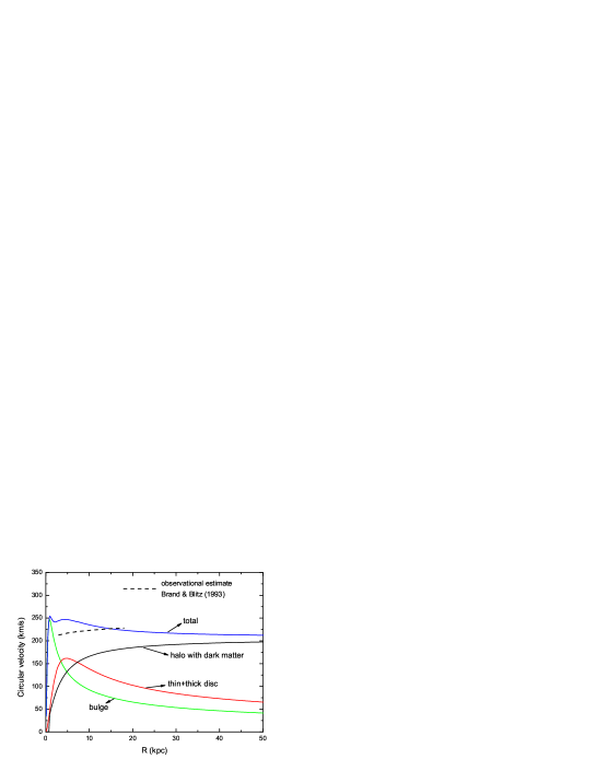
Fig. 1 demonstrates the influence of the Galactic model on the rotation curve of the Milky Way.
From the Galactic model, the total mass of the halo including dark matter is inside a sphere of radius 50 kpc. We only focus on the baryonic mass in the halo which is considered to be , constrained by the density of double white dwarfs (Yu & Jeffery, 2010). With the SFR adopted here, the baryonic mass in the bulge and disc is at least and respectively, implying that our model assumes no dark matter component localized to the bulge or the thin disc.
Combining the Galactic model and the mass of the Galactic components, the stellar density in the solar neighbourhood is , of which is in the thin disc, is in the thick disc, and is in the halo. This is consistent with the Hipparcos result, (Creze et al., 1998). The local dark matter density in our model is about .
2.2 Gravitational waves from double neutron stars
We calculate the GW strain amplitude from a single NS-NS binary by linearizing the equations of general relativity (Peters & Mathews, 1963; Landau & Lifshitz, 1975). We assume the following properties of a binary. 1) The masses of the two components are and respectively. Therefore the total mass , and the reduced mass . 2) The semi-major axis of the orbit is . 3) The eccentricity is . 4) From Kepler, the orbital separation and the angular velocity , where is the angle between the orbital separation and the -direction of an arbitrary Cartesian coordinate in the plane of the binary orbit, and is the gravitational constant. We take the direction perpendicular to the orbit plane and the origin is at the center of mass. Clearly, , where is the orbital period.
The components of the strain amplitude can be expressed as (Landau & Lifshitz, 1975)
| (26) |
where represents the second order differential of the mass-quadrupole tensor with respect to time, suffix denotes the direction, is the distance form the observer, and is the speed of light. Since the mass quadrupole tensor is
| (27) |
we have
| (28) |
From Eqs. 26, 27 and 28, it can be shown that the GW from a binary with circular orbit is monochromatic with frequency . When the orbit is eccentric, the wave becomes polychromatic and there is a frequency broadening in the GW signal.
The average power of the GW radiated from two point masses over one orbital period can be obtained by solving the third order differential of the mass-quadrupole tensor with respect to time (Peters & Mathews, 1963; Landau & Lifshitz, 1975). We quote the result
| (29) |
| (30) |
After Fourier analysis of Kepler motion, we obtain the power in the harmonic (Peters & Mathews, 1963)
| (31) |
| (32) |
where are Bessell functions of the first kind and . Since the sum of the power in each harmonic is equal to the total power emitted from the binary, we have
| (33) |
After a mathematical transformation based on the equations above (Nelemans et al., 2001; Yu & Jeffery, 2010), we obtain the strain amplitude in the vicinity of the Earth at GW frequency in the harmonic as
| (34) |
| (35) |
where is the so-called chirp mass. Eqs. 31, 32, 34, and 35 are the main equations used to calculate the power and strain amplitude of the GW signal from one individual NS-NS pair in frequency space. These equations also tell us that the power and strain amplitude of the GW signal from a binary consisting of two point-masses can be determined by four parameters - the chirp mass, orbital period, eccentricity and distance. In this paper, we refer to the first three as orbital parameters, and use the mass of each component instead of the chirp mass.
The energy flux of GW waves can be expressed as
| (36) |
where is the angular frequency. We define the spectral function of the energy flux as
| (37) |
where is the critical mass density of the present universe with km s-1 Mpc-1 being the Hubble constant (Freedman & Madore, 2010). We show the GW energy flux spectrum for selected cases to assist comparison with other work which uses this metric.
2.3 The sensitivity of eLISA
Evolved-LISA (eLISA) is designed as an updated version of LISA, a space-based GW detector, consisting of 1 mother and 2 daughter satellites flying in formation to form a Michelson-type Laser interferometer with an arm length of 1 km (see http://www.elisa-ngo.org/). Noise arises mainly from the displacement noise (including the noise caused by laser tracking system and other factors) and parasitic forces on the proof mass of an accelerometer (acceleration noise) (Larson et al., 2000)333The values of parameters to calculate the total noise can be found on http://www.elisa-ngo.org/.. We can convert the noise signal to an equivalent GW signal in frequency space by
| (38) |
where is the total strain noise spectral density, is the root spectral density and is the GW transfer function given by Larson et al. (2000). In the simulations, we take the displacement noise to be mHz-1/2 at 10 mHz, and the acceleration noise to be ms-2Hz-1/2 at 10 mHz. By comparison, the arm length of LISA would have been km. The displacement noise and acceleration noise would have been mHz-1/2 and ms-2Hz-1/2.
For a continuous monochromatic source, such as a NS-NS binary with a circular orbit, which is observed over a time , the root spectral density will appear in a Fourier spectrum as a single spectral line in the form (Larson et al., 2000)
| (39) |
So, for an observation time yr, the root strain amplitude spectral density Hz-1/2.
To demonstrate the detectability of the predicted GW signal due to the galactic DNS population, we show the expected eLISA sensitivity for S/N=1 in the figures in § 3.
2.4 Data reduction
We reduce the simulated GW signal by using its mean integrated value . To do this, we first choose a frequency interval which is greater than the interval used to compute the simulations (i.e. ). We then calculate the mean value of the strain amplitude and its standard deviation in this large frequency interval using
| (40) |
where represents the number of small-frequency intervals in the large frequency interval. In this paper, we take , so is also a function of frequency. We plot as a function of GW frequency in all figures unless specified otherwise. In each panel, we also show the maximum standard deviation which represents the maximum uncertainty in each large frequency interval in different cases.
| CEE() | CEA() | ||||||
|---|---|---|---|---|---|---|---|
| 1.0 | 0.5 | 1.3 | 1.5 | ||||
| Z=0.02 | SFH | IMF() | |||||
| Con | 1.5 | C1 | C3 | C25 | C27 | ||
| 2.5 | C2 | C4 | C26 | C28 | |||
| Exp | 1.5 | C5 | C7 | C29 | C31 | ||
| 2.5 | C6 | C8 | C30 | C32 | |||
| Inst | 1.5 | C9 | C11 | C33 | C35 | ||
| 2.5 | C10 | C12 | C34 | C36 | |||
| Z=0.001 | SFH | IMF() | |||||
| Con | 1.5 | C13 | C15 | C37 | C39 | ||
| 2.5 | C14 | C16 | C38 | C40 | |||
| Exp | 1.5 | C17 | C19 | C41 | C43 | ||
| 2.5 | C18 | C20 | C42 | C44 | |||
| Inst | 1.5 | C21 | C23 | C45 | C47 | ||
| 2.5 | C22 | C24 | C46 | C48 | |||
2.5 Computation procedure
In order to compute the superposition of the GW signal from the entire DNS population in the Galactic disc and compare the signal with the sensitivity of the proposed detectors, we need to know their birth rates, merger rates, present number, space, mass, eccentricity and orbital distributions. we have adopted the following procedure to obtain the above physical properties. For the Galactic thin disc with age , having a total mass 444We here neglect the interstellar medium which makes up about 20% of the thin disc mass (Robin et al., 2003).:
-
1.
For each star formation epoch in the disc, we calculate a sample distribution of coeval MS binaries having a total mass and generated by the four Monte-Carlo simulation parameters , , and .
-
2.
We follow the evolution of each primordial binary in a time grid consisting of many time intervals to establish the properties of DNSs formed from the above MS binaries up to . From the timescales from MS binary formation to DNS formation and from DNS formation to DNS merger, we can obtain the contribution function from each star formation epoch to the number of new-born and merged DNSs in a given time interval, as well as the total number of alive DNSs during that interval.
-
3.
By summing the contributions from all star formation epochs in the thin disc, we can obtain all the physical information of the DNS population, including birth and merger rates, present number, and distributions of orbital parameters.
- 4.
-
5.
We then calculate the total strain amplitude from the number and distance of DNSs in each frequency bin (for one year observation of e-LISA, see § 2.3). This yields a raw data of strain amplitude against the GW frequency.
-
6.
Finally, we use the method described in § 2.4 to reduce the raw data, producing a reduced relation between the strain amplitude and GW frequency.
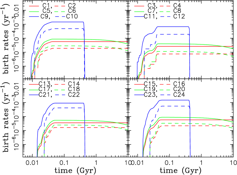
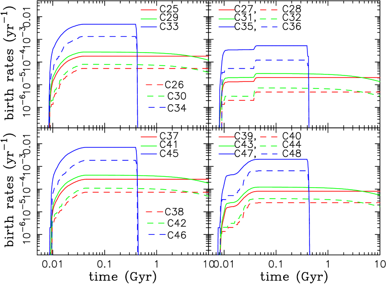
In our population synthesis simulation, we started with 16 primordial MS binaries, distributed equally between all 48 cases, and assume that Gyr. The parameters in the present study are SFH (Instantaneous, Continuous and Quasi-exponential), IMF ( and ), metallicity ( and 0.001), and two different CE evolution processes ( and ). For each CE formalism we adopt two parameters ( and 0.5, and 1.3). The 48 individual cases are labelled C1–C48 and are summarized in Table 3.
| Star Formation | CE Ejection | Present Birth Rate | Present Merger Rate | Total Number |
|---|---|---|---|---|
| yr-1 | yr-1 | |||
| Continuous | (C8 - C15) | (C8 - C15) | (C20 - C13) | |
| Continuous | (C32 - C37) | (C32 - C37) | (C32 - C37) | |
| Instantaneous | (C10,12,24 - C21) | |||
| Instantaneous | (C34,36,48 - C45) | (C36 - C45) |
3 Results
3.1 The double neutron-star population
3.1.1 Birth rates, merger rates, and numbers
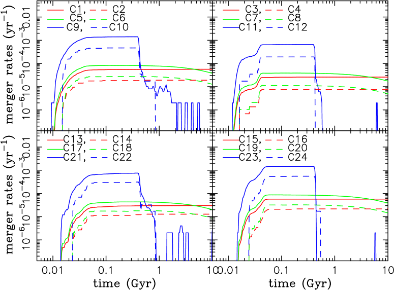
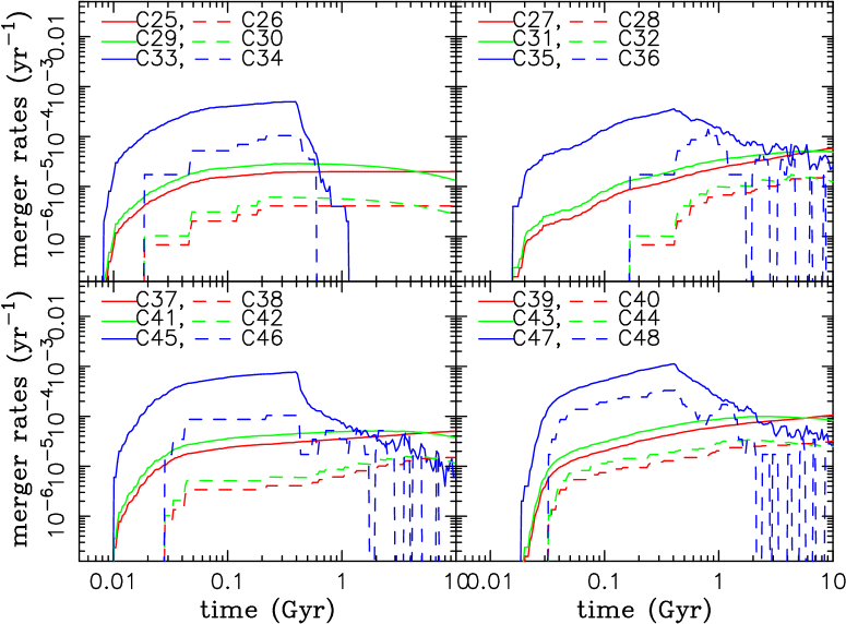
The total number of DNS is a crucial input parameter for calculating the integrated GW signal from the Galactic DNS population. The evolution of the birth and merger rates of DNS in the thin disc are shown in Figs. 2 and Figs. 3. There is a significant difference in total DNS numbers between the instantaneous SF model and the two other SF models. Since we assume that the response of descendent stars to a normalized star-formation epoch with the same input parameters is an intrinsic property, there should be a quasi-linear relation between the SF rate and the DNS birthrate. This can explain the different DNS birthrates in the three SF models. For example, the maximum DNS birthrate (1.46 ) in case C9 (instantaneous SF: SFR) is about 26 times that (5.72 ) in the case C1 (constant SF: SFR). The IMF affects the DNS birthrates in a similar way. Since the total number of initial MS binaries in the sample is constant (), a small value of the power-law index (i.e. ) increases the number of massive MS binaries and hence gives higher DNS birthrates.
Although metallicity and CE ejection coefficients have no direct impact on the initial number of MS binaries, they can significantly affect the orbital separation of a binary following a CE phase. If, after first CE ejection, the orbital separation is sufficiently small, the binary will not survive to become a DNS; this consequently reduces the DNS birthrate. However, if a binary can survive both first and second CE ejection, there is an increased probability of forming a very short-period compact binary. From Eqs. 4 and 6, either increasing or decreasing can, in principle, lead to small orbital separation after CE ejection, and lower the DNS birthrate. However, in the formalism, this is not true for low metallicity () , because the envelope of stars with low have smaller radii and usually have a smaller energy absorption, resulting in smaller mass loss via weaker stellar wind and in the formation of a massive core. From Eq. 6, a larger core mass helps a binary to survive, and thus increases the probability of DNS formation. In summary, under the formalism, a lower metallicity leads to larger core-mass and larger orbital separation, and increases the DNS formation probability. Decreasing the CE ejection coefficient results in a smaller orbital separation and lowers the DNS formation probability. In the formalism, the situation is not so obvious, but the orbital separation of a binary after a CE phase is also associated with the core-mass of primary. The DNS birthrate depends on a competition between the metallicity and the CE ejection coefficients.
Once a DNS has formed, its orbital separation and evolution is controlled by gravitational radiation and the magnetic field. The time scale for a MS binary to become a DNS is generally Myr. The merger time depends on the initial properties of the DNS (i.e. mass, orbital period, and eccentricity). Assuming the DNS orbital-period number distribution to be constant in logarithm, (), and the lifetime of an individual DNS to be (i.e. ), then the lifetime number distribution .
However, we argue that the DNS orbital-period number distribution is not simply a constant in logarithm. We compute the number evolution of the DNS population (see Fig. 4) using two methods to ensure consistency. First, we count the number from each star formation epoch. Second we calculate the integral of the difference between birth rate and merger rate. Our results show that the number of DNS in general depends on the total evolutionary mass of the thin disc. Small differences in the predicted number at the present epoch are found by using different metallicity and CE ejection coefficients.
Ranges in the current birth rates, merger rates and numbers of Galactic DNS assuming a thin-disc age of 10 Gyr as given by our binary-star population-synthesis calculations are shown in Table 4.
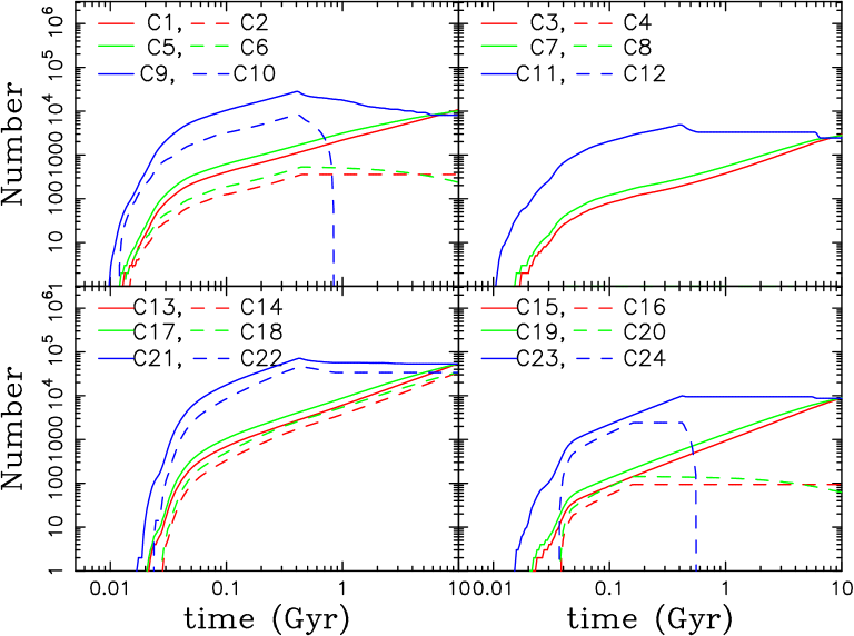
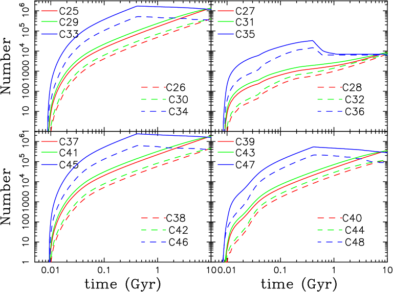
We draw attention to case C12 () in which, in our calculation and as a consequence of having orbital periods s, DNSs can be born and merge within the same computational time interval. This phenomenon leads to the total number of DNS always being zero in Fig. 4 (there is no blue dashed line in the panel showing C12). The similar cases C10 and C24 can also produce DNSs with short orbital periods ( s, but longer than in C12). The DNSs in these two cases also merge quickly, resulting in zero DNSs at the present age of the thin disc (10 Gyr). For comparison, as many as DNSs may be present at one time assuming a mechanism, that is times higher than assuming an mechanism. Even in the extreme case of instantaneous SF, the present number can be . This indicates that the mechanism can produce DNSs with orbital periods much longer than mechanism.
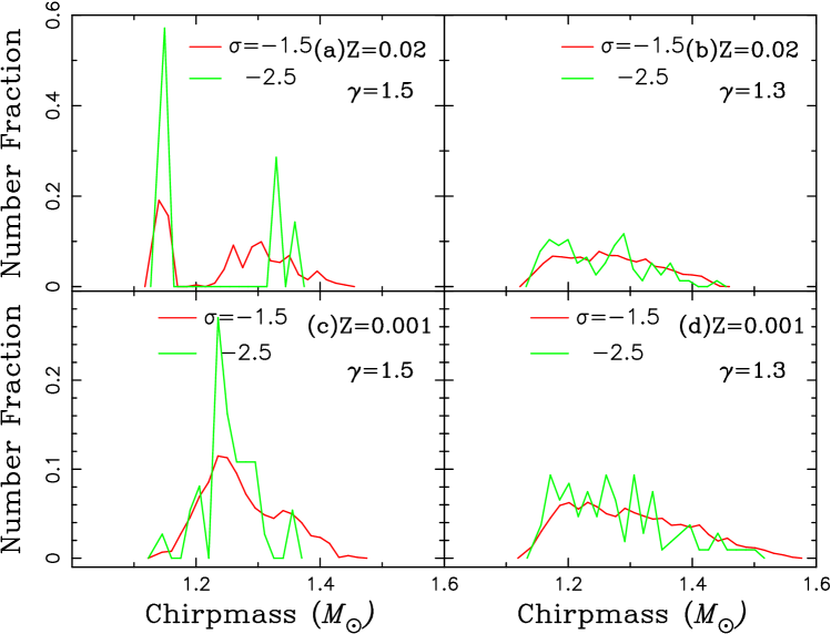
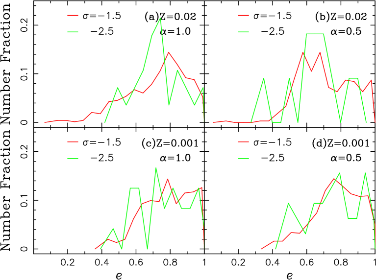
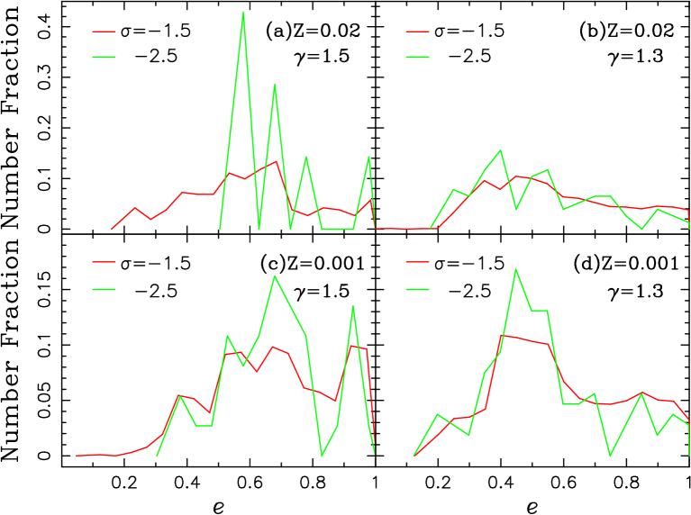
3.1.2 Chirpmass and eccentricity
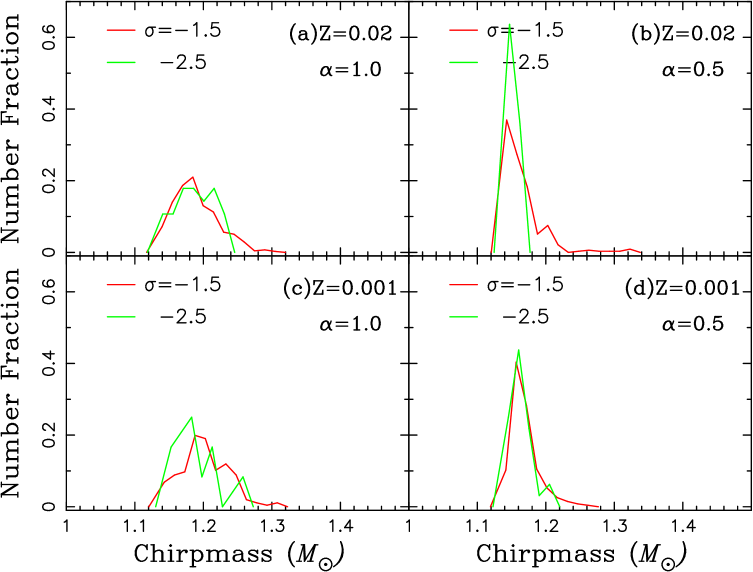
The distributions of chirp mass and eccentricity of the new-born DNS population are plotted in Figs. 5 and 6. Since our calculation is based on a number of coeval MS stars and SF has an overall effect on the calculation, the distributions of the physical variables of the DNS population (i.e. mass, eccentricity, and orbital period) are here only influenced by the metallicity, IMF and CE ejection coefficient. Since the masses of neutron stars described in Eq. 11 in our calculation are in the range , we expect their chirp masses (see Eq. 34) to lie in the range , as shown. Our results show that, in general, a lower or higher IMF index increases the fraction of DNS with higher chirp mass. Lower leads to less mass loss and eventually leaves a more massive core, and while a higher IMF index leads to more massive MS stars. In addition, we find that lower or higher tend to give a more concentrated distribution at smaller chirp mass. With no tidal interactions, the eccentricity distribution of the new-born DNS population is centered around assuming an mechanism and around assuming a mechanism. However, the eccentric orbits of the DNSs are likely to be circularized by gravitational wave radiation and/or tidal interaction during the common-envelope phase and subsequent evolution.
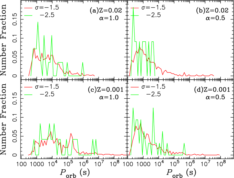
3.1.3 Orbital periods
The difference in the orbital period distributions due to the two CE ejection models is shown in Fig. 7. For the mechanism, most new-born DNSs have short orbital periods with a peak in the range s. Increasing the IMF index and/or gives more DNSs with longer orbital periods. The shortest orbital period in this model is about 200 s (, ), while the longest can be more than s (, , ). As argued already, the mechanism yields DNSs with longer orbital periods. The shortest orbital period in this model is about 3 000 s. In many cases the new-born DNSs can have orbital periods longer than s. These results are consistent with the values of birth and merger rates in Figs. 2 and 3.
3.1.4 Formation channels
The fractions of DNSs from different binary-star formation channnels are summarized for each model in Table 5. For -mechanism models it is found that most short-period DNSs ( s) come from the CE+CE channel, while longer period DNSs generally come from channels with at least once stable RLOF process. The dramatic decrease in the number of DNSs with short orbital periods ( s) in the -mechanism models is most likely due to the decrease of number of double CE ejection events. We find that the number fraction of DNSs with short orbital periods may be up to 10% in the two -mechanism models where double-CE events contribute over 80% of the DNSs.

| CE | CE+CE | RLOF+CE | other | |||
|---|---|---|---|---|---|---|
| Ejection | CE+RLOF | |||||
| Model | % | % | % | |||
| C1 | 1.0 | 0.02 | 87.2 | 1.6 | 11.2 | |
| C2 | 1.0 | 0.02 | 82.1 | 0.0 | 17.9 | |
| C3 | 0.5 | 0.02 | 93.6 | 1.0 | 5.4 | |
| C4 | 0.5 | 0.02 | 100.0 | 0.0 | 0.0 | |
| C13 | 1.0 | 0.001 | 58.0 | 15.9 | 26.1 | |
| C14 | 1.0 | 0.001 | 58.1 | 21.0 | 21.0 | |
| C15 | 0.5 | 0.001 | 95.3 | 1.6 | 3.1 | |
| C16 | 0.5 | 0.001 | 100.0 | 0.0 | 0.0 | |
| C25 | 1.3 | 0.02 | 44.4 | 55.5 | 0.1 | |
| C26 | 1.3 | 0.02 | 48.1 | 51.9 | 0.0 | |
| C27 | 1.5 | 0.02 | 94.3 | 4.6 | 1.1 | |
| C28 | 1.5 | 0.02 | 85.7 | 0.0 | 14.3 | |
| C37 | 1.3 | 0.001 | 37.9 | 60.4 | 1.7 | |
| C38 | 1.3 | 0.001 | 47.7 | 52.3 | 0.0 | |
| C39 | 1.5 | 0.001 | 64.7 | 33.8 | 2.5 | |
| C40 | 1.5 | 0.001 | 59.5 | 35.1 | 5.4 | |

3.1.5 The influence of kicks of neutron stars
As initialized, the kick velocities of neutron stars in our simulations obey a Maxwellian distribution with a maximum likelihood (in 3D) being km s-1. With a standard deviation of 190 km s-1, kick velocities can lie in the range 10 – 1200 km s-1. Since the new orbit of a binary is derived from the kick velocity (§ 2.1.4), it has a crucial influence on the distribution of eccentricity and orbital period. Kick velocities mean that about 95% of DNSs have eccentric orbits, with about 90% from supernova kicks, and about 5% from binary evolution. Our results indicate that young DNSs may have highly eccentric orbits, although gravitational wave radiation (and magnetic braking) tends to circularize the orbits during late evolution. By comparison, all the binary white dwarfs in the simulations of Yu & Jeffery (2010) have due to the tidal interaction and zero kick velocity.
Considering the extreme case of the neutron star velocity to be the sum of the maximum kick velocity and the Galactic rotation velocity, i.e. 1200+250 km s-1, their maximum speed is about 1.5 kpc Myr-1; the average will be closer to 268+250 km s kpc Myr-1. The measured GW strain depends on the distance; the change in strain over the course of one year due to neutron star kick velocities will be negligible.
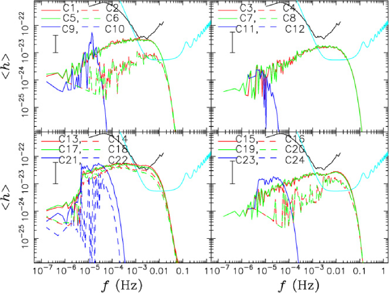
3.2 The GW strain-amplitude – frequency relation
Fig. 8. shows the DNS GW signal for each model in Table 3 as a strain- amplitude – frequency relation, reduced using the method described in § 2.4, so as to simplify the information contained. The probability to detect a GW signal from a DNS population using e-LISA, assuming an instantaneous SF model, is very low or close to to zero. If the SF rate is continuous or there is significant star formation in the recent past, we expect a high probability to detect a GW signal from a DNS population, assuming common-envelope ejection follows the mechanism. If CE ejection follows a mechanism, DNS GW detectability with e-LISA is also very low. The -mechanism can produce more DNSs at frequencies, but only at frequencies about 2 orders of magnitude lower than the best working frequency of e-LISA ( Hz).
Most of the strain-amplitude relations show oscillations in , sometimes with amplitudes of more than 1 dex. The DNS chirp masses in our calculation lie in the range , so can affect by a factor of 1.87. 95% of DNSs in our model lie at distances between 3.92 and 13.92 kpc, affecting the signal by a factor of up to 3.55. These two parameters are unlikely to explain the oscillation. The distribution of DNS orbital periods should be the most important factor. This can be understood as follows.
We first assume that any probability distribution function can be fitted by a normal or multi-normal distribution, so that the simplest distribution function is the normal distribution. We apply this distribution to the orbital periods to understand the relation. The frequency distribution can be expressed as
| (41) |
If the distribution of is normal, then
| (42) |
To find the extrema of the function to be summed in Eq. 42, we set its first derivative with respect to frequency equal to zero. After rearranging,
| (43) |
where and . If , the frequency distribution may have maximum values, and the interval between two successive maxima is . If , the interval becomes negligible.
The total strain amplitude in one frequency bin has been calculated as the sum of the strain amplitude of those binaries in the frequency bin, expressed as
| (44) |
If we assume the binaries in a frequency bin have similar chirp mass, the above equation becomes
| (45) |
where is a constant. Combining with Eq.42, we obtain an expression for the strain amplitude generated from DNS binaries with normally distributed orbital periods:
| (46) |
To find the extrema, we take the derivative of the function in the sum and obtain
| (47) |
which has the solutions . The properties of are similar to those of . In addition, when , .
Consequently, if the orbital periods satisfy a perfect normal distribution, an oscillation can appear in the relation under the condition that neighboring frequencies coincide with extrema of . However, since the orbital periods are most likely the sum of normal distributions with different and , the frequencies where the strain amplitudes have extrema relate to and .
This analysis demonstrates the following. If a population of Galactic DNS has a relatively large distribution of orbital period (large ), it will generate a smooth GW background. However, with small , or a tight distribution of period, we see a set of harmonics in the frequency range Hz. All the DNSs in the sample are effectively“in tune”. With larger this effect is smeared out. This means that under some conditions (e.g. ), the oscillation of space caused by the GW radiation from a DNS population at low frequencies can be regularly enhanced. We note that the oscillation in our simulations is hardly detectable by eLISA.
For comparison, Fig. 8 also shows the reduced GW signal from double white dwarfs (DWDs) simulated by the method in Yu & Jeffery (2010). The signals from DWDs occupy (20%) of the observation frequency intervals for one year of observation, and they should have a different polarization pattern from the signal from DNSs. This means that future observations should be able to distinguish the DNS and DWD signals.
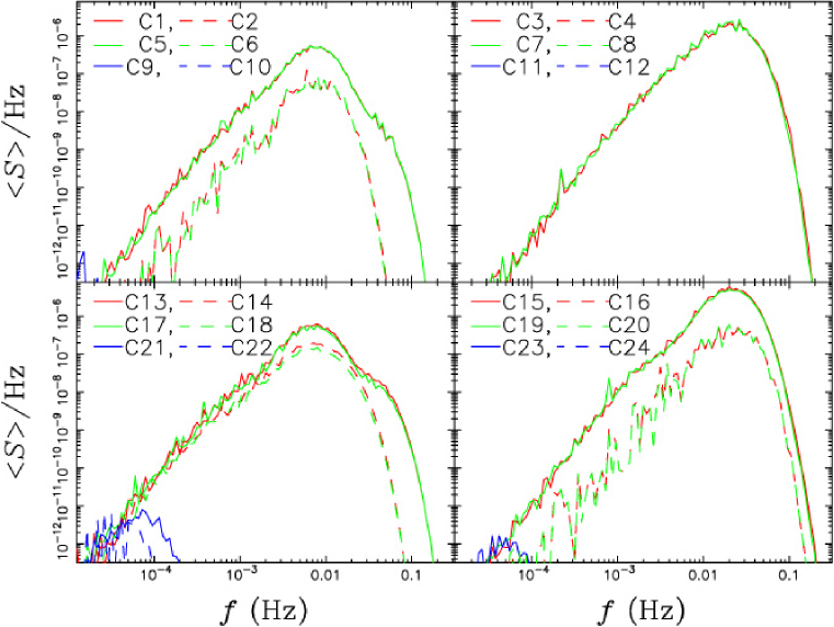
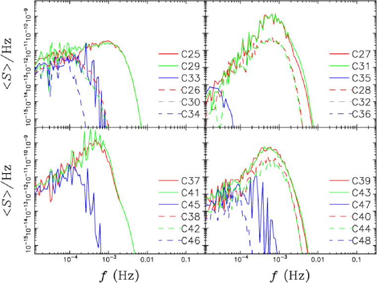
Since several authors plot gravitational energy flux rather than strain amplitude, Fig. 9 shows the same information as Fig. 8 for DNS in terms of the spectral energy distrubution , calculated from Eq. 37 and reduced using the method in § 2.4.
3.3 Discrete Gravitational-Wave Signals
In previous work (Yu & Jeffery, 2010, 2011) we have used the term ‘resolved’ GW systems to refer to those binaries in which all of the GW strain measured within a single frequency interval over a given integration period arises from a single system. Since all of the DNSs in our simulation are in eccentric orbits, their GW emission may be spread over many frequency intervals. Thus the concept of a ‘resolved’ DNS may not be useful. We prefer to use the term ‘discrete GW signal’ to represent a frequency interval that contains a GW signal greater than some noise threshold over a given observation period. The number of such signals serves as a proxy to estimate what might be expected from future observations.
We hence define the number of discrete GW signals exceeding the noise threshold, where the subscript defines the confidence level. Thus means that frequency intervals show a GW signal with S/N1, gives the number of frequency intervals with S/N3, and so on. The results are listed in Table 6. We find that a lower metallicity and a larger IMF power-law index give a higher probability for the detection of a GW signal. The highest probability occurs in case C15 (, , and constant SF rate). This case gives 57195 discrete signals at and 19933 discrete signals at . The detection-probability for a discrete GW signal is much lower in a mechanism model than in an equivalent mechanism model. For -mechanism models, the highest probability occurs for C31 (, , and exponential SF rate), with 75 signals at and none at .
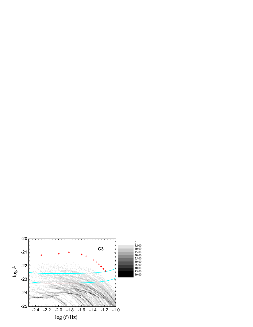

Some DNSs with large eccentricities may generate a detectable GW signal at multiple harmonics of the orbital frequency. For example, in simulation C3, a DNS with , s, and kpc generates GW signals at the fundamental frequency 0.00504 Hz and its harmonics (i.e. 0.01008 Hz, 0.01512 Hz, 0.02016 Hz, …) at . The numerical error in the frequencies is less than 0.02%. The detection of GW signals in harmonic series would help to constrain the DNS orbital parameters. Note that in addition to the signal caused by the DNS in this example, there is another weak GW signal at frequencies of 0.02016, 0.02520, 0.04032, 0.0504 and 0.06552 Hz (4, 5, 8, 10 and 13) respectively caused by other DNSs.
In order to investigate the potential number of ‘resolvable’ DNSs, Table 7 shows the numbers () of DNSs which have at least one detectable GW harmonic. This number is not equivalent to the number which contribute to the GW signals in Table 6, where a GW signal may exceed the detection criterion due to the combined strain of two or more DNS at the same frequency. Table 7 does not include DNS which generate GW signals below the detector threshold. Hence, for example, cases C15 and C39 show 57195 and 56 GW signals (at ), representing the combined contributions from about 500 - 950 and 1 - 13 DNSs in each case. In case C39, no individual DNS generates a detectable GW signal. Figure 11 illustrates the number of DNSs per frequency bin as a function of GW frequency in cases C15 and C39. We finally emphasize that the GW signals in Table 6 come from a much smaller number of individual sources as indicated by the numbers of resolved sources shown in Table 7.
| Case | Case | ||||||
|---|---|---|---|---|---|---|---|
| C1 | 24467 | 11766 | 7253 | C13 | 37270 | 19660 | 11770 |
| C2 | 1127 | 625 | 399 | C14 | 29129 | 12777 | 6654 |
| C3 | 16406 | 8789 | 5869 | C15 | 57195 | 30689 | 19933 |
| C4 | 0 | 0 | 0 | C16 | 1622 | 759 | 476 |
| C5 | 23518 | 11454 | 7133 | C17 | 34057 | 16982 | 9692 |
| C6 | 870 | 482 | 306 | C18 | 23131 | 9397 | 4632 |
| C7 | 16371 | 8435 | 5643 | C19 | 54618 | 29213 | 19249 |
| C8 | 0 | 0 | 0 | C20 | 1492 | 693 | 449 |
| C9 | 0 | 0 | 0 | C21 | 0 | 0 | 0 |
| C10 | 0 | 0 | 0 | C22 | 0 | 0 | 0 |
| C11 | 0 | 0 | 0 | C23 | 0 | 0 | 0 |
| C12 | 0 | 0 | 0 | C24 | 0 | 0 | 0 |
| C25 | 0 | 0 | 0 | C37 | 24 | 0 | 0 |
| C26 | 0 | 0 | 0 | C38 | 2 | 0 | 0 |
| C27 | 60 | 3 | 0 | C39 | 56 | 0 | 0 |
| C28 | 0 | 0 | 0 | C40 | 0 | 0 | 0 |
| C29 | 0 | 0 | 0 | C41 | 14 | 4 | 0 |
| C30 | 0 | 0 | 0 | C42 | 2 | 0 | 0 |
| C31 | 75 | 3 | 0 | C43 | 26 | 0 | 0 |
| C32 | 0 | 0 | 0 | C44 | 0 | 0 | 0 |
| C33 | 0 | 0 | 0 | C45 | 0 | 0 | 0 |
| C34 | 0 | 0 | 0 | C46 | 0 | 0 | 0 |
| C35 | 0 | 0 | 0 | C47 | 0 | 0 | 0 |
| C36 | 0 | 0 | 0 | C48 | 0 | 0 | 0 |
| Case | Case | ||||||
|---|---|---|---|---|---|---|---|
| C1 | 1273 | 927 | 743 | C13 | 2434 | 1446 | 1031 |
| C2 | 45 | 42 | 35 | C14 | 1471 | 812 | 546 |
| C3 | 543 | 487 | 429 | C15 | 1473 | 1291 | 1115 |
| C4 | 0 | 0 | 0 | C16 | 38 | 33 | 28 |
| C5 | 1220 | 896 | 729 | C17 | 2005 | 1194 | 835 |
| C6 | 34 | 32 | 26 | C18 | 1049 | 585 | 379 |
| C7 | 538 | 474 | 409 | C19 | 1412 | 1226 | 1078 |
| C8 | 0 | 0 | 0 | C20 | 35 | 30 | 26 |
| C9 | 0 | 0 | 0 | C21 | 0 | 0 | 0 |
| C10 | 0 | 0 | 0 | C22 | 0 | 0 | 0 |
| C11 | 0 | 0 | 0 | C23 | 0 | 0 | 0 |
| C12 | 0 | 0 | 0 | C24 | 0 | 0 | 0 |
| C25 | 0 | 0 | 0 | C37 | 2 | 0 | 0 |
| C26 | 0 | 0 | 0 | C38 | 1 | 0 | 0 |
| C27 | 7 | 1 | 0 | C39 | 3 | 0 | 0 |
| C28 | 0 | 0 | 0 | C40 | 0 | 0 | 0 |
| C29 | 0 | 0 | 0 | C41 | 2 | 1 | 0 |
| C30 | 0 | 0 | 0 | C42 | 2 | 0 | 0 |
| C31 | 11 | 1 | 0 | C43 | 1 | 0 | 0 |
| C32 | 0 | 0 | 0 | C44 | 0 | 0 | 0 |
| C33 | 0 | 0 | 0 | C45 | 0 | 0 | 0 |
| C34 | 0 | 0 | 0 | C46 | 0 | 0 | 0 |
| C35 | 0 | 0 | 0 | C47 | 0 | 0 | 0 |
| C36 | 0 | 0 | 0 | C48 | 0 | 0 | 0 |
3.4 GW signal from the Galactic components
Amongst our experiments, cases C2, C4, C6, C8, C26, C28, C30 and C32 better represent the bulge and thin disc for SF history, IMF and metallicity. However, due to the lower total mass of the bulge (Robin et al., 2003; Belczynski et al., 2010b; Yu & Jeffery, 2010), the number of GW signals from the DNSs in the bulge should be less than that in the thin disc by a factor of . Since the thick disc has a much smaller total stellar mass ( (Robin et al., 2003; Yu & Jeffery, 2010)), the GW signal from DNSs in the thick disk should be less than that in the thin disc by a factor of about 20. The halo has a quite different SF history (SF only at early epochs), IMF (), and metallicity () from the thin disc, but would have a similar stellar mass ( ). Numerical experiments C21, C23, C45 and C47 better reflect conditions in the halo. Our results show that very rare GW signals from the DNSs in the halo can be observed, which support the results of Belczynski et al. (2010b). Note that the influence of distance may be negligible.
In the model of Yu & Jeffery (2010), the mean distances and standard deviations of stars in the bulge, the disc, and the halo are, respectively, kpc, kpc, and kpc. In fact, a realistic GW signal will lie somewhere between the cases studied. For example, if the mean metallicity of the thin disc lies between 0.001 and 0.02 (Panter et al., 2008; Belczynski et al., 2010b), a more realistic case would be a combination of C2 and C14, or C4 and C16 and so on. We here approximate the GW contribution from the Galaxy as a whole by correcting the thin disc contribution () for the bulge (), thick disk (), and halo ().
Belczynski et al. (2010b) concluded that the number of resolved DNSs in their population synthesis model should be about 6, which is consistent with the results of Nelemans et al. (2001). For an eLISA-type observatory, and assuming case C2 (Table 4) is approximately representative of the Galaxy as a whole, one year of observation will yield about 1633 observable DNS-induced GW signals, 906 signals at S/N=3, and 577 at S/N=5.
4 Discussion
We have used an evolutionary model to simulate the birth and merger rates and the total number of DNSs in the Galactic thin disc. Our results on rates and total number are roughly consistent with the observational constraints (Kalogera et al., 2004) and with binary-star formation and evolution theory calculated by others (Nelemans et al., 2001; Dominik et al., 2012). However, Nelemans et al. (2001) only give an optimistic value for the rates and number assuming the mechanism. Kalogera et al. (2004) report results based on observation and statistical theory; they neglect the dependency of the rates and number on initial conditions and stellar evolution parameters. Dominik et al. (2012) investigated the influence of metallicity and the mechanism CE ejection coefficient, they did not investigate different SF and IMF models. In this paper we have systematically investigated the influence of all these initial conditions and stellar evolution parameters on the rates and total number of DNSs.
Using the binary-star population synthesis model, we have calculated the stable GW emission from the long-lived DNS population which may be observable by (for example) eLISA in the frequency range Hz. In fact, these calculations can be used to estimate the GW signal from other Galactic components, i.e. the bulge, the thick disc, and the halo. The SF rates in the bulge and thin disc are most likely to be continuous, and both share a common metallicity (). The power-law indices of the IMF in these regions are also similar, being in the bulge and in the thin disc for stars with mass (Zoccali et al., 2000; Kroupa et al., 1993; Kroupa, 2001; Robin et al., 2003).
Rosado (2011) adopts an analytic approach to study the GW background from binary systems, and concludes that no background signal generated by DNSs and DWDs is detectable in the frequency band of ground-based GW detectors. Our calculations support this conclusion.
Since the GW signal from DNSs is significantly affected by SF history, recent SF regions in the bulge and spiral arms of the Galaxy may contain many GW sources. By comparison, although the Large and Small Magellanic Clouds may have experienced bursts of star formation peaking roughly 2, 0.5, 0.1 and 0.012 Gyr ago (Harris & Zaritsky, 2009) and 2.5, 0.4, and 0.06 Gyr ago (Harris & Zaritsky, 2004), respectively, the low Magellanic-Cloud SF rate of roughly implies the GW signal from Magellanic-Cloud DNSs should be negligible compared with that in the Galaxy.
A caveat affecting all of our simulations is that, in practice, the number of detectable DNS present in the Galaxy at any one time is small. Even in cases where the number of GW signals exceeds , Table 7 shows that these arise from a relatively small number of ‘resolvable’ DNS, with eccentric systems producing signals at multiple harmonics. The DNS eccentricity distribution in our model is essentially that defined by the common-envelope interaction physics, followed by tidal evolution as discussed in §2.1.2. While observations show that highly eccentric DNS do exist at long period (cf. Table 1), tidal evolution to short-period systems is not tested. Detailed models for the influence of kick velocity distribution and galactic structure on the orbital parameters of DNSs and therefore their GW signal are also needed to extend our model to different types of galaxy. More seriously, since the predicted GW signal is based on small numbers amongst which the eccentricity distribution is determined by a Monte-Carlo distribution applied to the parent population, uncertainties on numbers in Table 5 are more likely to scale as , the numbers of DNS in Table 6, than as .
5 Conclusion
Using the methods of binary-star population synthesis, we have investigated the Galactic double neutron-star (DNS) population as a function of initial mass function, star-formation history, metallicity and common-envelope physics. The parameter space explored is larger than covered previously, and includes a volume corresponding to best estimates of the present-day Galaxy. We have computed the gravitational-wave (GW) signal that would be generated by these theoretical populations, including the multi-frequency signal generated by DNSs in elliptical orbits. We have also explored the probability of likelihood of detecting GW from DNS from a conceptual space-borne GW observatory (eLISA). The main conclusions are:
(1) Observable GW from double neutron stars are more likely in low metallicity environments, in environments where there is a high proportion of massive stars, and in regions of recent star formation. The first two statements are relatively obvious; low metallicity produces less luminous and, hence, smaller giants, so that binaries are more tightly bound at the point of common-envelope ejection, whilst a higher IMF power-law index produces more high mass stars, and therefore more DNS. If the galactic metallicity is reduced from to , the number of observable GW signals from DNS increases by a factor up to in the two continuous star formation models (e.g. C6 and C18), and consistent with Belczynski et al. (2010a). The influence of the IMF is even stronger than that of metallicity; increasing the power-law index from to increases the number of observable GW signals from DNS from 0 to 2434–57195 1- detections in the frequency range Hz. The fraction of DNS arising from star formation within the last Gyr is almost 100% of the total DNS population.
(2) Observable GW from DNS reflect the physics of the common-envelope ejection mechanism. If conservation of energy dominates (formalism), DNS GW are more likely to be observed than if conservation of angular momentum (formalism) dominates the physics. The peak frequency at which the average strain amplitude has a maximum value in these two mechanisms is also different. The peak frequency for the formalism is in the range of 0.001 – 0.01 Hz, while the peak frequency for the formalism is in the range of Hz. Observation of the DNS GW spectrum will therefore help to constrain common-envelope ejection physics.
(3) Young DNSs most likely have eccentric orbits resulting mostly from kick velocities imparted during supernova collapse and partly binary evolution. This creates a harmonic structure in the GW radiation of DNSs.
(4) Current observations indicate the most realistic values for the physical parameters in the Galactic disc correspond with our cases C2 and C6, i.e. and either constant (C2) or exponentially decreasing (C6) star formation. We therefore expect that one year of observation with a GW observatory such as eLISA will detect approximately 01600 observable GW signals caused by DNSs at S/N1, 0900 signals at S/N3, and 0570 signals at S/N5 in the Galaxy between 10-5 and 1 Hz, coming from about 065, 060 and 050 resolved DNS.
Acknowledgments
This work was supported by the National Science Foundation of China (NSFC), Grant No. 11303054 and 11261140641, the Chinese Ministry of Science and Technology under the State Key Development Program for Basic Research, Grant No. 2013CB837900, the Projects of International Cooperation and Exchange, the key research program of the Chinese Academy of Sciences (CAS), Grant No. KJZD-EW-T01. This work was also supported by the Open Project Program of the key Laboratory of Radio Astronomy, CAS and Scientific Research Foundation of the Ministry of Education. Research at the Armagh Observatory is grant-aided by the N. Ireland Department of Culture, Arts and Leisure.
References
- Allen et al. (2012) Allen B., Anderson W. G., Brady P. R., Brown D. A., Creighton J. D. E., 2012, Phys. Rev. D, 85, 122006
- Allen et al. (1999) Allen B., Blackburn J. K., Brady P. R., Creighton J. D., Creighton T., Droz S., Gillespie A. D., Hughes S. A., Kawamura S., Lyons T. T., Mason J. E., Owen B. J., Raab F. J., Regehr M. W., Sathyaprakash B. S., Savage R. L., Whitcomb S., Wiseman A. G., 1999, Physical Review Letters, 83, 1498
- Arzoumanian et al. (2002) Arzoumanian Z., Chernoff D. F., Cordes J. M., 2002, ApJ, 568, 289
- Barish & Weiss (1999) Barish B. C., Weiss R., 1999, Physics Today, 52, 44
- Belczynski et al. (2010a) Belczynski K., Benacquista M., Bulik T., 2010a, ApJ, 725, 816
- Belczynski et al. (2010b) Belczynski K., Benacquista M., Bulik T., 2010b, ApJ, 725, 816
- Belczynski et al. (2010) Belczynski K., Dominik M., Bulik T., O’Shaughnessy R., Fryer C., Holz D. E., 2010, ApJ, 715, L138
- Belczynski et al. (2008) Belczynski K., Kalogera V., Rasio F. A., Taam R. E., Zezas A., Bulik T., Maccarone T. J., Ivanova N., 2008, ApJS, 174, 223
- Brand & Blitz (1993) Brand J., Blitz L., 1993, A&A, 275, 67
- Brandt & Podsiadlowski (1995) Brandt N., Podsiadlowski P., 1995, MNRAS, 274, 461
- Burgay et al. (2003) Burgay M., D’Amico N., Possenti A., Manchester R. N., Lyne A. G., Joshi B. C., McLaughlin M. A., Kramer M., Sarkissian J. M., Camilo F., Kalogera V., Kim C., Lorimer D. R., 2003, Nature, 426, 531
- Caldwell & Ostriker (1981) Caldwell J. A. R., Ostriker J. P., 1981, ApJ, 251, 61
- Campbell (1984) Campbell C. G., 1984, MNRAS, 207, 433
- Champion et al. (2004) Champion D. J., Lorimer D. R., McLaughlin M. A., Cordes J. M., Arzoumanian Z., Weisberg J. M., Taylor J. H., 2004, MNRAS, 350, L61
- Creze et al. (1998) Creze M., Chereul E., Bienayme O., Pichon C., 1998, A&A, 329, 920
- Diehl et al. (2006) Diehl R., Halloin H., Kretschmer K., Lichti G. G., Schönfelder V., Strong A. W., von Kienlin A., Wang W., Jean P., Knödlseder J., Roques J., Weidenspointner G., Schanne S., Hartmann D. H., Winkler C., Wunderer C., 2006, Nature, 439, 45
- Dominik et al. (2012) Dominik M., Belczynski K., Fryer C., Holz D. E., Berti E., Bulik T., Mandel I., O’Shaughnessy R., 2012, ApJ, 759, 52
- Eggleton (1983) Eggleton P. P., 1983, ApJ, 268, 368
- Faulkner et al. (2005) Faulkner A. J., Kramer M., Lyne A. G., Manchester R. N., McLaughlin M. A., Stairs I. H., Hobbs G., Possenti A., Lorimer D. R., D’Amico N., Camilo F., Burgay M., 2005, ApJ, 618, L119
- Faulkner (1971) Faulkner J., 1971, ApJ, 170, L99+
- Freedman & Madore (2010) Freedman W. L., Madore B. F., 2010, ARA&A, 48, 673
- Freudenreich (1998) Freudenreich H. T., 1998, ApJ, 492, 495
- Fryer & Kalogera (1997) Fryer C., Kalogera V., 1997, ApJ, 489, 244
- Goldberg & Mazeh (1994) Goldberg D., Mazeh T., 1994, A&A, 282, 801
- Han (1998) Han Z., 1998, MNRAS, 296, 1019
- Han et al. (1995) Han Z., Podsiadlowski P., Eggleton P. P., 1995, MNRAS, 272, 800
- Han et al. (2003) Han Z., Podsiadlowski P., Maxted P. F. L., Marsh T. R., 2003, MNRAS, 341, 669
- Hansen & Phinney (1997) Hansen B. M. S., Phinney E. S., 1997, MNRAS, 291, 569
- Harris & Zaritsky (2004) Harris J., Zaritsky D., 2004, AJ, 127, 1531
- Harris & Zaritsky (2009) Harris J., Zaritsky D., 2009, AJ, 138, 1243
- Heggie (1975) Heggie D. C., 1975, MNRAS, 173, 729
- Hobbs et al. (2005) Hobbs G., Lorimer D. R., Lyne A. G., Kramer M., 2005, MNRAS, 360, 974
- Hulse & Taylor (1975) Hulse R. A., Taylor J. H., 1975, ApJ, 195, L51
- Hurley et al. (2000) Hurley J. R., Pols O. R., Tout C. A., 2000, MNRAS, 315, 543
- Hurley et al. (2002) Hurley J. R., Tout C. A., Pols O. R., 2002, MNRAS, 329, 897
- Hut (1981) Hut P., 1981, A&A, 99, 126
- Iben & Tutukov (1996) Iben Jr. I., Tutukov A. V., 1996, ApJ, 456, 738
- Jahreiß & Wielen (1997) Jahreiß H., Wielen R., 1997, in R. E. Schielicke ed., Astronomische Gesellschaft Abstract Series Vol. 13 of Astronomische Gesellschaft Abstract Series, HIPPARCOS and the nearby stars. pp 43–+
- Kalogera et al. (2004) Kalogera V., Kim C., Lorimer D. R., Burgay M., D’Amico N., Possenti A., Manchester R. N., Lyne A. G., Joshi B. C., McLaughlin M. A., Kramer M., Sarkissian J. M., Camilo F., 2004, ApJ, 601, L179
- Kalogera et al. (2001) Kalogera V., Narayan R., Spergel D. N., Taylor J. H., 2001, ApJ, 556, 340
- Kramer et al. (2004) Kramer M., Backer D. C., Cordes J. M., Lazio T. J. W., Stappers B. W., Johnston S., 2004, New A Rev., 48, 993
- Kramer & Stairs (2008) Kramer M., Stairs I. H., 2008, ARA&A, 46, 541
- Kroupa (2001) Kroupa P., 2001, MNRAS, 322, 231
- Kroupa et al. (1993) Kroupa P., Tout C. A., Gilmore G., 1993, MNRAS, 262, 545
- Lai et al. (1995) Lai D., Bildsten L., Kaspi V. M., 1995, ApJ, 452, 819
- Lai et al. (2001) Lai D., Chernoff D. F., Cordes J. M., 2001, ApJ, 549, 1111
- Landau & Lifshitz (1975) Landau L. D., Lifshitz E. M., 1975, The classical theory of fields. Course of theoretical physics - Pergamon International Library of Science, Technology, Engineering and Social Studies, Oxford: Pergamon Press, 1975, 4th rev.engl.ed.
- Langer (2012) Langer N., 2012, ARA&A, 50, 107
- Larson et al. (2000) Larson S. L., Hiscock W. A., Hellings R. W., 2000, Phys. Rev. D, 62, 062001
- Lattimer & Prakash (2007) Lattimer J. M., Prakash M., 2007, Phys. Rep., 442, 109
- Lorimer (2008) Lorimer D. R., 2008, Living Reviews in Relativity, 11, 8
- Lorimer et al. (2006) Lorimer D. R., Stairs I. H., Freire P. C., Cordes J. M., Camilo F., Faulkner A. J., Lyne A. G., Nice D. J., et al. 2006, ApJ, 640, 428
- Lyne et al. (1982) Lyne A. G., Anderson B., Salter M. J., 1982, MNRAS, 201, 503
- Lyne et al. (2004) Lyne A. G., Burgay M., Kramer M., Possenti A., Manchester R. N., Camilo F., McLaughlin M. A., Lorimer D. R., D’Amico N., Joshi B. C., Reynolds J., Freire P. C. C., 2004, Science, 303, 1153
- Lyne et al. (2000) Lyne A. G., Camilo F., Manchester R. N., Bell J. F., Kaspi V. M., D’Amico N., McKay N. P. F., Crawford F., Morris D. J., Sheppard D. C., Stairs I. H., 2000, MNRAS, 312, 698
- Lyne & Lorimer (1994) Lyne A. G., Lorimer D. R., 1994, Nature, 369, 127
- Lyne & McKenna (1989) Lyne A. G., McKenna J., 1989, Nature, 340, 367
- Mazeh et al. (1992) Mazeh T., Goldberg D., Duquennoy A., Mayor M., 1992, ApJ, 401, 265
- Minkowski (1970) Minkowski R., 1970, PASP, 82, 470
- Miyamoto & Nagai (1975) Miyamoto M., Nagai R., 1975, PASJ, 27, 533
- Nelemans & Tout (2005) Nelemans G., Tout C. A., 2005, MNRAS, 356, 753
- Nelemans et al. (2000) Nelemans G., Verbunt F., Yungelson L. R., Portegies Zwart S. F., 2000, A&A, 360, 1011
- Nelemans et al. (2001) Nelemans G., Yungelson L. R., Portegies Zwart S. F., 2001, A&A, 375, 890
- Nelemans et al. (2004) Nelemans G., Yungelson L. R., Portegies Zwart S. F., 2004, MNRAS, 349, 181
- Nice et al. (1996) Nice D. J., Sayer R. W., Taylor J. H., 1996, ApJ, 466, L87
- Nordhaus et al. (2012) Nordhaus J., Brandt T. D., Burrows A., Almgren A., 2012, MNRAS, 423, 1805
- Osłowski et al. (2011) Osłowski S., Bulik T., Gondek-Rosińska D., Belczyński K., 2011, MNRAS, 413, 461
- Paczynski (1990) Paczynski B., 1990, ApJ, 348, 485
- Paczyński & Ziółkowski (1967) Paczyński B., Ziółkowski J., 1967, Acta Astronomica, 17, 7
- Panter et al. (2008) Panter B., Jimenez R., Heavens A. F., Charlot S., 2008, MNRAS, 391, 1117
- Peters & Mathews (1963) Peters P. C., Mathews J., 1963, Physical Review, 131, 435
- Popper (1980) Popper D. M., 1980, ARA&A, 18, 115
- Postnov & Yungelson (2006) Postnov K. A., Yungelson L. R., 2006, Living Reviews in Relativity, 9, 6
- Prince et al. (1991) Prince T. A., Anderson S. B., Kulkarni S. R., Wolszczan A., 1991, ApJ, 374, L41
- Rappaport et al. (1983) Rappaport S., Verbunt F., Joss P. C., 1983, ApJ, 275, 713
- Rasio et al. (1996) Rasio F. A., Tout C. A., Lubow S. H., Livio M., 1996, ApJ, 470, 1187
- Refsdal et al. (1974) Refsdal S., Roth M. L., Weigert A., 1974, A&A, 36, 113
- Regimbau & de Freitas Pacheco (2006) Regimbau T., de Freitas Pacheco J. A., 2006, ApJ, 642, 455
- Ricci & Brillet (1997) Ricci F., Brillet A., 1997, Annual Review of Nuclear and Particle Science, 47, 111
- Robin et al. (2003) Robin A. C., Reylé C., Derrière S., Picaud S., 2003, A&A, 409, 523
- Rosado (2011) Rosado P. A., 2011, Phys. Rev. D, 84, 084004
- Sana et al. (2012) Sana H., de Mink S. E., de Koter A., Langer N., Evans C. J., Gieles M., Gosset E., Izzard R. G., Le Bouquin J.-B., Schneider F. R. N., 2012, Science, 337, 444
- Skumanich (1972) Skumanich A., 1972, ApJ, 171, 565
- Smith et al. (1978) Smith L. F., Biermann P., Mezger P. G., 1978, A&A, 66, 65
- Timmes et al. (1997) Timmes F. X., Diehl R., Hartmann D. H., 1997, ApJ, 479, 760
- Webbink (1984) Webbink R. F., 1984, ApJ, 277, 355
- Webbink (2008) Webbink R. F., 2008, in E. F. Milone, D. A. Leahy, & D. W. Hobill ed., Astrophysics and Space Science Library Vol. 352 of Astrophysics and Space Science Library, Common Envelope Evolution Redux. pp 233–+
- Wielen et al. (1983) Wielen R., Jahreiß H., Krüger R., 1983, in A. G. D. Philip & A. R. Upgren ed., IAU Colloq. 76: Nearby Stars and the Stellar Luminosity Function The Determination of the Luminosity Function of Nearby Stars. pp 163–170
- Wolszczan (1991) Wolszczan A., 1991, Nature, 350, 688
- Yu & Jeffery (2010) Yu S., Jeffery C. S., 2010, A&A, 521, A85+
- Yu & Jeffery (2011) Yu S., Jeffery C. S., 2011, MNRAS, 417, 1392
- Zahn (1977) Zahn J., 1977, A&A, 57, 383
- Zangrilli et al. (1997) Zangrilli L., Tout C. A., Bianchini A., 1997, MNRAS, 289, 59
- Zhu et al. (2013) Zhu X.-J., Howell E. J., Blair D. G., Zhu Z.-H., 2013, MNRAS, 431, 882
- Zoccali et al. (2000) Zoccali M., Cassisi S., Frogel J. A., Gould A., Ortolani S., Renzini A., Rich R. M., Stephens A. W., 2000, ApJ, 530, 418