Abstract.
We study reproducing kernels, and associated reproducing kernel Hilbert
spaces (RKHSs) ℋ ℋ \mathscr{H} V 𝑉 V V 𝑉 V ℋ ℋ \mathscr{H} V 𝑉 V δ x subscript 𝛿 𝑥 \delta_{x} x 𝑥 x V 𝑉 V V 𝑉 V
1. Introduction
A reproducing kernel Hilbert space (RKHS) is a Hilbert space ℋ ℋ \mathscr{H} V 𝑉 V f ∈ ℋ 𝑓 ℋ f\in\mathscr{H} ℋ ℋ \mathscr{H} x ∈ V 𝑥 𝑉 x\in V f ∈ ℋ 𝑓 ℋ f\in\mathscr{H} f ( x ) 𝑓 𝑥 f\left(x\right) ℋ ℋ \mathscr{H} f 𝑓 f k x subscript 𝑘 𝑥 k_{x} ℋ ℋ \mathscr{H}
The RKHSs have been studied extensively since the pioneering papers
by Aronszajn in the 1940ties, see e.g., [Aro43 , Aro48 ] . They
further play an important role in the theory of partial differential
operators (PDO); for example as Green’s functions of second order
elliptic PDOs; see e.g., [Nel57 , HKL+ ] . Other applications include
engineering, physics, machine-learning theory (see [KH11 , SZ09 , CS02 ] ),
stochastic processes (e.g., Gaussian free fields), numerical analysis,
and more. See, e.g., [AD93 , ABDdS93 , AD92 , AJSV13 , AJV14 ] . Also,
see [LB04 , HQKL10 , ZXZ12 , LP11 , Vul13 , SS13 , HN14 ] .
But the literature so far has focused on the theory of kernel functions
defined on continuous domains, either domains in Euclidean space,
or complex domains in one or more variables. For these cases, the
Dirac δ x subscript 𝛿 𝑥 \delta_{x} ℋ ℋ \mathscr{H} δ x subscript 𝛿 𝑥 \delta_{x} ℋ ℋ \mathscr{H}
An illustration from neural networks: An Extreme Learning Machine
(ELM) is a neural network configuration in which a hidden layer of
weights are randomly sampled (see e.g., [RW06 ] ), and the object
is then to determine analytically resulting output layer weights.
Hence ELM may be thought of as an approximation to a network with
infinite number of hidden units.
Here we consider the discrete case, i.e., RKHSs of functions defined
on a prescribed countable infinite discrete set V 𝑉 V ℋ ℋ \mathscr{H} δ x subscript 𝛿 𝑥 \delta_{x} x ∈ V 𝑥 𝑉 x\in V ℋ ℋ \mathscr{H}
Our setting is a given positive definite function k 𝑘 k V × V 𝑉 𝑉 V\times V V 𝑉 V ℋ ( = ℋ ( k ) ) annotated ℋ absent ℋ 𝑘 \mathscr{H}\left(=\mathscr{H}\left(k\right)\right) 2.12 3.18 4.13 V 𝑉 V ℋ ℋ \mathscr{H} 3.5 3.20 4.5 4.7 4.11 4.12
The paper is organized as follows: Section 2 2.12 ℋ ℋ \mathscr{H} 3 4 3 V × V 𝑉 𝑉 V\times V 4 G 𝐺 G 4.5 V 𝑉 V 4.7 4.11 4.15
A positive definite kernel k 𝑘 k universal [CMPY08 ]
if, every continuous function, on a compact subset of the input space,
can be uniformly approximated by sections of the kernel, i.e., by
continuous functions in the RKHS. In Theorem 4.13 k c subscript 𝑘 𝑐 k_{c} G 𝐺 G G 𝐺 G c 𝑐 c G 𝐺 G
2. Discrete RKHSs
Definition 2.1 .
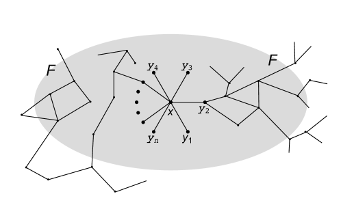
Let V 𝑉 V ℱ ( V ) ℱ 𝑉 \mathscr{F}\left(V\right) finite subsets of V 𝑉 V k : V × V → ℂ : 𝑘 → 𝑉 𝑉 ℂ k:V\times V\rightarrow\mathbb{C} positive definite , if
∑ ∑ ( x , y ) ∈ F × F k ( x , y ) c x ¯ c y ≥ 0 𝑥 𝑦 𝐹 𝐹 𝑘 𝑥 𝑦 ¯ subscript 𝑐 𝑥 subscript 𝑐 𝑦 0 \underset{\left(x,y\right)\in F\times F}{\sum\sum}k\left(x,y\right)\overline{c_{x}}c_{y}\geq 0 (2.1)
holds for all coefficients { c x } x ∈ F ⊂ ℂ subscript subscript 𝑐 𝑥 𝑥 𝐹 ℂ \{c_{x}\}_{x\in F}\subset\mathbb{C} F ∈ ℱ ( V ) 𝐹 ℱ 𝑉 F\in\mathscr{F}\left(V\right)
Definition 2.2 .
Fix a set V 𝑉 V
(1)
For all x ∈ V 𝑥 𝑉 x\in V
k x := k ( ⋅ , x ) : V → ℂ : assign subscript 𝑘 𝑥 𝑘 ⋅ 𝑥 → 𝑉 ℂ k_{x}:=k\left(\cdot,x\right):V\rightarrow\mathbb{C} (2.2)
as a function on V 𝑉 V
(2)
Let ℋ := ℋ ( k ) assign ℋ ℋ 𝑘 \mathscr{H}:=\mathscr{H}\left(k\right) s p a n { k x : x ∈ V } 𝑠 𝑝 𝑎 𝑛 conditional-set subscript 𝑘 𝑥 𝑥 𝑉 span\left\{k_{x}:x\in V\right\}
⟨ ∑ c x k x , ∑ d y k y ⟩ ℋ := ∑ ∑ c x ¯ d y k ( x , y ) assign subscript subscript 𝑐 𝑥 subscript 𝑘 𝑥 subscript 𝑑 𝑦 subscript 𝑘 𝑦
ℋ ¯ subscript 𝑐 𝑥 subscript 𝑑 𝑦 𝑘 𝑥 𝑦 \left\langle\sum c_{x}k_{x},\sum d_{y}k_{y}\right\rangle_{\mathscr{H}}:=\sum\sum\overline{c_{x}}d_{y}k\left(x,y\right) (2.3)
modulo the subspace of functions of zero ℋ ℋ \mathscr{H} ℋ ℋ \mathscr{H}
⟨ k x , φ ⟩ ℋ = φ ( x ) , ∀ x ∈ V , ∀ φ ∈ ℋ . formulae-sequence subscript subscript 𝑘 𝑥 𝜑
ℋ 𝜑 𝑥 formulae-sequence for-all 𝑥 𝑉 for-all 𝜑 ℋ \left\langle k_{x},\varphi\right\rangle_{\mathscr{H}}=\varphi\left(x\right),\;\forall x\in V,\>\forall\varphi\in\mathscr{H}. (2.4)
Note. The summations in (2.3 2.3 ℋ = ℋ ( k ) ℋ ℋ 𝑘 \mathscr{H}=\mathscr{H}\left(k\right)
(3)
If F ∈ ℱ ( V ) 𝐹 ℱ 𝑉 F\in\mathscr{F}\left(V\right) ℋ F = closed span { k x } x ∈ F ⊂ ℋ subscript ℋ 𝐹 closed span subscript subscript 𝑘 𝑥 𝑥 𝐹 ℋ \mathscr{H}_{F}=\text{closed\>\ span}\{k_{x}\}_{x\in F}\subset\mathscr{H} F 𝐹 F
P F := the orthogonal projection onto ℋ F . assign subscript 𝑃 𝐹 the orthogonal projection onto ℋ F P_{F}:=\text{the orthogonal projection onto $\mathscr{H}_{F}$}. (2.5)
(4)
For F ∈ ℱ ( V ) 𝐹 ℱ 𝑉 F\in\mathscr{F}\left(V\right)
K F := ( k ( x , y ) ) ( x , y ) ∈ F × F assign subscript 𝐾 𝐹 subscript 𝑘 𝑥 𝑦 𝑥 𝑦 𝐹 𝐹 K_{F}:=\left(k\left(x,y\right)\right)_{\left(x,y\right)\in F\times F} (2.6)
as a # F × # F # 𝐹 # 𝐹 \#F\times\#F
Remark 2.3 .
It follows from the above that reproducing kernel Hilbert spaces (RKHS)
arise from a given positive definite kernel k 𝑘 k 2.2 k 𝑘 k [OST13 , ST12 , Str10 ] ),
band-limited L 2 superscript 𝐿 2 L^{2}
Our focus here is on discrete analogues of the classical RKHSs from
real or complex analysis. These discrete RKHSs in turn are dictated
by applications, and their features are quite different from those
of their continuous counter parts.
Definition 2.4 .
The RKHS ℋ = ℋ ( k ) ℋ ℋ 𝑘 \mathscr{H}=\mathscr{H}\left(k\right) discrete mass property (ℋ ℋ \mathscr{H} discrete RKHS ), if δ x ∈ ℋ subscript 𝛿 𝑥 ℋ \delta_{x}\in\mathscr{H} x ∈ V 𝑥 𝑉 x\in V δ x ( y ) = { 1 if x = y 0 if x ≠ y subscript 𝛿 𝑥 𝑦 cases 1 if 𝑥 𝑦 0 if x ≠ y \delta_{x}\left(y\right)=\begin{cases}1&\text{if }x=y\\
0&\text{if $x\neq y$}\end{cases} x ∈ V 𝑥 𝑉 x\in V
Lemma 2.5 .
Let F ∈ ℱ ( V ) 𝐹 ℱ 𝑉 F\in\mathscr{F}\left(V\right) x 1 ∈ F subscript 𝑥 1 𝐹 x_{1}\in F δ x 1 ∈ ℋ subscript 𝛿 subscript 𝑥 1 ℋ \delta_{x_{1}}\in\mathscr{H}
P F ( δ x 1 ) ( ⋅ ) = ∑ y ∈ F ( K F − 1 δ x 1 ) ( y ) k y ( ⋅ ) . subscript 𝑃 𝐹 subscript 𝛿 subscript 𝑥 1 ⋅ subscript 𝑦 𝐹 superscript subscript 𝐾 𝐹 1 subscript 𝛿 subscript 𝑥 1 𝑦 subscript 𝑘 𝑦 ⋅ P_{F}\left(\delta_{x_{1}}\right)\left(\cdot\right)=\sum_{y\in F}\left(K_{F}^{-1}\delta_{x_{1}}\right)\left(y\right)k_{y}\left(\cdot\right). (2.7)
Proof.
Show that
δ x − ∑ y ∈ F ( K F − 1 δ x 1 ) ( y ) k y ( ⋅ ) ∈ ℋ F ⟂ . subscript 𝛿 𝑥 subscript 𝑦 𝐹 superscript subscript 𝐾 𝐹 1 subscript 𝛿 subscript 𝑥 1 𝑦 subscript 𝑘 𝑦 ⋅ superscript subscript ℋ 𝐹 perpendicular-to \delta_{x}-\sum_{y\in F}\left(K_{F}^{-1}\delta_{x_{1}}\right)\left(y\right)k_{y}\left(\cdot\right)\in\mathscr{H}_{F}^{\perp}. (2.8)
The remaining part follows easily from this.
(The notation ( ℋ F ) ⟂ superscript subscript ℋ 𝐹 perpendicular-to \left(\mathscr{H}_{F}\right)^{\perp} ℋ ⊖ ℋ F = { φ ∈ ℋ | ⟨ f , φ ⟩ ℋ = 0 , ∀ f ∈ ℋ F } symmetric-difference ℋ subscript ℋ 𝐹 conditional-set 𝜑 ℋ formulae-sequence subscript 𝑓 𝜑
ℋ 0 for-all 𝑓 subscript ℋ 𝐹 \mathscr{H}\ominus\mathscr{H}_{F}=\left\{\varphi\in\mathscr{H}\>\big{|}\>\left\langle f,\varphi\right\rangle_{\mathscr{H}}=0,\;\forall f\in\mathscr{H}_{F}\right\}
Lemma 2.6 .
Using Dirac’s bra-ket, and ket-bra notation (for
rank-one operators), the orthogonal projection onto ℋ F subscript ℋ 𝐹 \mathscr{H}_{F}
P F = ∑ y ∈ F | k y ⟩ ⟨ k y ∗ | ; P_{F}=\sum_{y\in F}\left|k_{y}\left\rangle\right\langle k_{y}^{*}\right|; (2.9)
where
k x ∗ := ∑ y ∈ F ( K F − 1 ) y x k y assign superscript subscript 𝑘 𝑥 subscript 𝑦 𝐹 subscript superscript subscript 𝐾 𝐹 1 𝑦 𝑥 subscript 𝑘 𝑦 k_{x}^{*}:=\sum_{y\in F}\left(K_{F}^{-1}\right)_{yx}k_{y} (2.10)
is the dual vector to k x subscript 𝑘 𝑥 k_{x} x ∈ V 𝑥 𝑉 x\in V
Proof.
Let k x ∗ superscript subscript 𝑘 𝑥 k_{x}^{*} 2.10
⟨ k x ∗ , k z ⟩ ℋ subscript superscript subscript 𝑘 𝑥 subscript 𝑘 𝑧
ℋ \displaystyle\left\langle k_{x}^{*},k_{z}\right\rangle_{\mathscr{H}} = \displaystyle= ∑ y ∈ F ⟨ ( K F − 1 ) y x k y , k z ⟩ ℋ subscript 𝑦 𝐹 subscript subscript superscript subscript 𝐾 𝐹 1 𝑦 𝑥 subscript 𝑘 𝑦 subscript 𝑘 𝑧
ℋ \displaystyle\sum_{y\in F}\left\langle\left(K_{F}^{-1}\right)_{yx}k_{y},k_{z}\right\rangle_{\mathscr{H}}
= \displaystyle= ∑ y ∈ F ( K F − 1 ) x y ⟨ k y , k z ⟩ ℋ subscript 𝑦 𝐹 subscript superscript subscript 𝐾 𝐹 1 𝑥 𝑦 subscript subscript 𝑘 𝑦 subscript 𝑘 𝑧
ℋ \displaystyle\sum_{y\in F}\left(K_{F}^{-1}\right)_{xy}\left\langle k_{y},k_{z}\right\rangle_{\mathscr{H}}
= \displaystyle= ∑ y ∈ F ( K F − 1 ) x y ( K F ) y z = δ x , z , subscript 𝑦 𝐹 subscript superscript subscript 𝐾 𝐹 1 𝑥 𝑦 subscript subscript 𝐾 𝐹 𝑦 𝑧 subscript 𝛿 𝑥 𝑧
\displaystyle\sum_{y\in F}\left(K_{F}^{-1}\right)_{xy}\left(K_{F}\right)_{yz}=\delta_{x,z},
i.e., k x ∗ superscript subscript 𝑘 𝑥 k_{x}^{*} k x subscript 𝑘 𝑥 k_{x} x ∈ V 𝑥 𝑉 x\in V
For f ∈ ℋ 𝑓 ℋ f\in\mathscr{H} F ∈ ℱ ( V ) 𝐹 ℱ 𝑉 F\in\mathscr{F}\left(V\right)
∑ y ∈ F | k y ⟩ ⟨ k y ∗ | f \displaystyle\sum_{y\in F}\left|k_{y}\left\rangle\right\langle k_{y}^{*}\right|f = \displaystyle= ∑ y ∈ F ⟨ k y ∗ , f ⟩ ℋ k y subscript 𝑦 𝐹 subscript superscript subscript 𝑘 𝑦 𝑓
ℋ subscript 𝑘 𝑦 \displaystyle\sum_{y\in F}\left\langle k_{y}^{*},f\right\rangle_{\mathscr{H}}k_{y}
= \displaystyle= ∑ ∑ ( y , z ) ∈ F × F ( K F − 1 ) z , y ⟨ k z , f ⟩ ℋ 𝑦 𝑧 𝐹 𝐹 subscript superscript subscript 𝐾 𝐹 1 𝑧 𝑦
subscript subscript 𝑘 𝑧 𝑓
ℋ \displaystyle\underset{\left(y,z\right)\in F\times F}{\sum\sum}\left(K_{F}^{-1}\right)_{z,y}\left\langle k_{z},f\right\rangle_{\mathscr{H}}
= \displaystyle= P F f . subscript 𝑃 𝐹 𝑓 \displaystyle P_{F}f.
This yields the orthogonal projection realized as stated in (2.9
Now, applying (2.9 δ x 1 subscript 𝛿 subscript 𝑥 1 \delta_{x_{1}}
P F ( δ x 1 ) subscript 𝑃 𝐹 subscript 𝛿 subscript 𝑥 1 \displaystyle P_{F}\left(\delta_{x_{1}}\right) = \displaystyle= ∑ y ∈ F ⟨ k y ∗ , δ x 1 ⟩ ℋ k y subscript 𝑦 𝐹 subscript superscript subscript 𝑘 𝑦 subscript 𝛿 subscript 𝑥 1
ℋ subscript 𝑘 𝑦 \displaystyle\sum_{y\in F}\left\langle k_{y}^{*},\delta_{x_{1}}\right\rangle_{\mathscr{H}}k_{y}
= \displaystyle= ∑ y ∈ F ( ∑ z ∈ F ( K F − 1 ) y z ⟨ k z , δ x 1 ⟩ ℋ ) k y subscript 𝑦 𝐹 subscript 𝑧 𝐹 subscript superscript subscript 𝐾 𝐹 1 𝑦 𝑧 subscript subscript 𝑘 𝑧 subscript 𝛿 subscript 𝑥 1
ℋ subscript 𝑘 𝑦 \displaystyle\sum_{y\in F}\left(\sum_{z\in F}\left(K_{F}^{-1}\right)_{yz}\left\langle k_{z},\delta_{x_{1}}\right\rangle_{\mathscr{H}}\right)k_{y}
= \displaystyle= ∑ y ∈ F ( ∑ z ∈ F ( K F − 1 ) y z δ x 1 ( z ) ) k y subscript 𝑦 𝐹 subscript 𝑧 𝐹 subscript superscript subscript 𝐾 𝐹 1 𝑦 𝑧 subscript 𝛿 subscript 𝑥 1 𝑧 subscript 𝑘 𝑦 \displaystyle\sum_{y\in F}\left(\sum_{z\in F}\left(K_{F}^{-1}\right)_{yz}\delta_{x_{1}}\left(z\right)\right)k_{y}
= \displaystyle= ∑ y ∈ F ( K F − 1 δ x 1 ) ( y ) k y , subscript 𝑦 𝐹 superscript subscript 𝐾 𝐹 1 subscript 𝛿 subscript 𝑥 1 𝑦 subscript 𝑘 𝑦 \displaystyle\sum_{y\in F}\left(K_{F}^{-1}\delta_{x_{1}}\right)\left(y\right)k_{y},
where
( K F − 1 δ x 1 ) ( y ) := ∑ z ∈ F ( K F − 1 ) y z δ x 1 ( z ) . assign superscript subscript 𝐾 𝐹 1 subscript 𝛿 subscript 𝑥 1 𝑦 subscript 𝑧 𝐹 subscript superscript subscript 𝐾 𝐹 1 𝑦 𝑧 subscript 𝛿 subscript 𝑥 1 𝑧 \left(K_{F}^{-1}\delta_{x_{1}}\right)\left(y\right):=\sum_{z\in F}\left(K_{F}^{-1}\right)_{yz}\delta_{x_{1}}\left(z\right).
This verifies (2.7
Remark 2.7 .
Note a slight abuse of notations: We make formally sense of the expressions
for P F ( δ x ) subscript 𝑃 𝐹 subscript 𝛿 𝑥 P_{F}(\delta_{x}) 2.7 δ x subscript 𝛿 𝑥 \delta_{x} ℋ ℋ \mathscr{H} F 𝐹 F P F ( δ x ) ∈ ℋ subscript 𝑃 𝐹 subscript 𝛿 𝑥 ℋ P_{F}(\delta_{x})\in\mathscr{H} δ x subscript 𝛿 𝑥 \delta_{x} ℋ ℋ \mathscr{H} 2.18 2.12
Lemma 2.8 .
Let F ∈ ℱ ( V ) 𝐹 ℱ 𝑉 F\in\mathscr{F}\left(V\right) x 1 ∈ F subscript 𝑥 1 𝐹 x_{1}\in F
( K F − 1 δ x 1 ) ( x 1 ) = ‖ P F δ x 1 ‖ ℋ 2 . superscript subscript 𝐾 𝐹 1 subscript 𝛿 subscript 𝑥 1 subscript 𝑥 1 superscript subscript norm subscript 𝑃 𝐹 subscript 𝛿 subscript 𝑥 1 ℋ 2 \left(K_{F}^{-1}\delta_{x_{1}}\right)\left(x_{1}\right)=\left\|P_{F}\delta_{x_{1}}\right\|_{\mathscr{H}}^{2}. (2.11)
Proof.
Setting ζ ( F ) := K F − 1 ( δ x 1 ) assign superscript 𝜁 𝐹 superscript subscript 𝐾 𝐹 1 subscript 𝛿 subscript 𝑥 1 \zeta^{\left(F\right)}:=K_{F}^{-1}\left(\delta_{x_{1}}\right)
P F ( δ x 1 ) = ∑ y ∈ F ζ ( F ) ( y ) k F ( ⋅ , y ) subscript 𝑃 𝐹 subscript 𝛿 subscript 𝑥 1 subscript 𝑦 𝐹 superscript 𝜁 𝐹 𝑦 subscript 𝑘 𝐹 ⋅ 𝑦 P_{F}\left(\delta_{x_{1}}\right)=\sum_{y\in F}\zeta^{\left(F\right)}\left(y\right)k_{F}\left(\cdot,y\right)
and for all z ∈ F 𝑧 𝐹 z\in F
∑ z ∈ F ζ ( F ) ( z ) P F ( δ x 1 ) ( z ) ⏟ ζ ( F ) ( x 1 ) superscript 𝜁 𝐹 subscript 𝑥 1 ⏟ subscript 𝑧 𝐹 superscript 𝜁 𝐹 𝑧 subscript 𝑃 𝐹 subscript 𝛿 subscript 𝑥 1 𝑧 \displaystyle\underset{\zeta^{\left(F\right)}\left(x_{1}\right)}{\underbrace{\sum_{z\in F}\zeta^{\left(F\right)}\left(z\right)P_{F}\left(\delta_{x_{1}}\right)\left(z\right)}} = \displaystyle= ∑ F ∑ F ζ ( F ) ( z ) ζ ( F ) ( y ) k F ( z , y ) subscript 𝐹 subscript 𝐹 superscript 𝜁 𝐹 𝑧 superscript 𝜁 𝐹 𝑦 subscript 𝑘 𝐹 𝑧 𝑦 \displaystyle\sum_{F}\sum_{F}\zeta^{\left(F\right)}\left(z\right)\zeta^{\left(F\right)}\left(y\right)k_{F}\left(z,y\right)
= \displaystyle= ‖ P F δ x 1 ‖ ℋ 2 . superscript subscript norm subscript 𝑃 𝐹 subscript 𝛿 subscript 𝑥 1 ℋ 2 \displaystyle\left\|P_{F}\delta_{x_{1}}\right\|_{\mathscr{H}}^{2}.
Note the LHS of (2 2.6
‖ P F δ x 1 ‖ ℋ 2 superscript subscript norm subscript 𝑃 𝐹 subscript 𝛿 subscript 𝑥 1 ℋ 2 \displaystyle\left\|P_{F}\delta_{x_{1}}\right\|_{\mathscr{H}}^{2} = \displaystyle= ⟨ P F δ x 1 , δ x 1 ⟩ ℋ subscript subscript 𝑃 𝐹 subscript 𝛿 subscript 𝑥 1 subscript 𝛿 subscript 𝑥 1
ℋ \displaystyle\left\langle P_{F}\delta_{x_{1}},\delta_{x_{1}}\right\rangle_{\mathscr{H}}
= \displaystyle= ∑ y ∈ F ( K F − 1 δ x 1 ) ( y ) ⟨ k y , δ x 1 ⟩ ℋ subscript 𝑦 𝐹 superscript subscript 𝐾 𝐹 1 subscript 𝛿 subscript 𝑥 1 𝑦 subscript subscript 𝑘 𝑦 subscript 𝛿 subscript 𝑥 1
ℋ \displaystyle\sum_{y\in F}\left(K_{F}^{-1}\delta_{x_{1}}\right)\left(y\right)\left\langle k_{y},\delta_{x_{1}}\right\rangle_{\mathscr{H}}
= \displaystyle= ( K F − 1 δ x 1 ) ( x 1 ) = K F − 1 ( x 1 , x 1 ) . superscript subscript 𝐾 𝐹 1 subscript 𝛿 subscript 𝑥 1 subscript 𝑥 1 superscript subscript 𝐾 𝐹 1 subscript 𝑥 1 subscript 𝑥 1 \displaystyle\left(K_{F}^{-1}\delta_{x_{1}}\right)\left(x_{1}\right)=K_{F}^{-1}\left(x_{1},x_{1}\right).
∎
Corollary 2.9 .
If δ x 1 ∈ ℋ subscript 𝛿 subscript 𝑥 1 ℋ \delta_{x_{1}}\in\mathscr{H} 2.12
sup F ∈ ℱ ( V ) ( K F − 1 δ x 1 ) ( x 1 ) = ‖ δ x 1 ‖ ℋ 2 . subscript supremum 𝐹 ℱ 𝑉 superscript subscript 𝐾 𝐹 1 subscript 𝛿 subscript 𝑥 1 subscript 𝑥 1 superscript subscript norm subscript 𝛿 subscript 𝑥 1 ℋ 2 \sup_{F\in\mathscr{F}\left(V\right)}\left(K_{F}^{-1}\delta_{x_{1}}\right)\left(x_{1}\right)=\left\|\delta_{x_{1}}\right\|_{\mathscr{H}}^{2}. (2.13)
The following condition is satisfied in some examples, but not all:
Corollary 2.10 .
∃ F ∈ ℱ ( V ) 𝐹 ℱ 𝑉 \exists F\in\mathscr{F}\left(V\right) s.t. δ x 1 ∈ ℋ F subscript 𝛿 subscript 𝑥 1 subscript ℋ 𝐹 \delta_{x_{1}}\in\mathscr{H}_{F} ⟺ ⟺ \Longleftrightarrow
K F ′ − 1 ( δ x 1 ) ( x 1 ) = K F − 1 ( δ x 1 ) ( x 1 ) superscript subscript 𝐾 superscript 𝐹 ′ 1 subscript 𝛿 subscript 𝑥 1 subscript 𝑥 1 superscript subscript 𝐾 𝐹 1 subscript 𝛿 subscript 𝑥 1 subscript 𝑥 1 K_{F^{\prime}}^{-1}\left(\delta_{x_{1}}\right)\left(x_{1}\right)=K_{F}^{-1}\left(\delta_{x_{1}}\right)\left(x_{1}\right)
for all F ′ ⊃ F 𝐹 superscript 𝐹 ′ F^{\prime}\supset F
Corollary 2.11 (Monotonicity).
If F 𝐹 F F ′ superscript 𝐹 ′ F^{\prime} ℱ ( V ) ℱ 𝑉 \mathscr{F}\left(V\right) F ⊂ F ′ 𝐹 superscript 𝐹 ′ F\subset F^{\prime}
( K F − 1 δ x 1 ) ( x 1 ) ≤ ( K F ′ − 1 δ x 1 ) ( x 1 ) superscript subscript 𝐾 𝐹 1 subscript 𝛿 subscript 𝑥 1 subscript 𝑥 1 superscript subscript 𝐾 superscript 𝐹 ′ 1 subscript 𝛿 subscript 𝑥 1 subscript 𝑥 1 \left(K_{F}^{-1}\delta_{x_{1}}\right)\left(x_{1}\right)\leq\left(K_{F^{\prime}}^{-1}\delta_{x_{1}}\right)\left(x_{1}\right) (2.14)
and
lim F ↗ V ( K F − 1 δ x 1 ) ( x 1 ) = ‖ δ x 1 ‖ ℋ 2 . subscript ↗ 𝐹 𝑉 superscript subscript 𝐾 𝐹 1 subscript 𝛿 subscript 𝑥 1 subscript 𝑥 1 superscript subscript norm subscript 𝛿 subscript 𝑥 1 ℋ 2 \lim_{F\nearrow V}\left(K_{F}^{-1}\delta_{x_{1}}\right)\left(x_{1}\right)=\left\|\delta_{x_{1}}\right\|_{\mathscr{H}}^{2}. (2.15)
Proof.
By (2.11
( K F − 1 δ x 1 ) ( x 1 ) = ‖ P F δ x 1 ‖ ℋ 2 . superscript subscript 𝐾 𝐹 1 subscript 𝛿 subscript 𝑥 1 subscript 𝑥 1 superscript subscript norm subscript 𝑃 𝐹 subscript 𝛿 subscript 𝑥 1 ℋ 2 \left(K_{F}^{-1}\delta_{x_{1}}\right)\left(x_{1}\right)=\left\|P_{F}\delta_{x_{1}}\right\|_{\mathscr{H}}^{2}.
Since ℋ F ⊂ ℋ F ′ subscript ℋ 𝐹 subscript ℋ superscript 𝐹 ′ \mathscr{H}_{F}\subset\mathscr{H}_{F^{\prime}} P F P F ′ = P F subscript 𝑃 𝐹 subscript 𝑃 superscript 𝐹 ′ subscript 𝑃 𝐹 P_{F}P_{F^{\prime}}=P_{F}
‖ P F δ x 1 ‖ ℋ 2 = ‖ P F P F ′ δ x 1 ‖ ℋ 2 ≤ ‖ P F ′ δ x 1 ‖ ℋ 2 superscript subscript norm subscript 𝑃 𝐹 subscript 𝛿 subscript 𝑥 1 ℋ 2 superscript subscript norm subscript 𝑃 𝐹 subscript 𝑃 superscript 𝐹 ′ subscript 𝛿 subscript 𝑥 1 ℋ 2 superscript subscript norm subscript 𝑃 superscript 𝐹 ′ subscript 𝛿 subscript 𝑥 1 ℋ 2 \left\|P_{F}\delta_{x_{1}}\right\|_{\mathscr{H}}^{2}=\left\|P_{F}P_{F^{\prime}}\delta_{x_{1}}\right\|_{\mathscr{H}}^{2}\leq\left\|P_{F^{\prime}}\delta_{x_{1}}\right\|_{\mathscr{H}}^{2}
i.e.,
( K F − 1 δ x 1 ) ( x 1 ) ≤ ( K F ′ − 1 δ x 1 ) ( x 1 ) . superscript subscript 𝐾 𝐹 1 subscript 𝛿 subscript 𝑥 1 subscript 𝑥 1 superscript subscript 𝐾 superscript 𝐹 ′ 1 subscript 𝛿 subscript 𝑥 1 subscript 𝑥 1 \left(K_{F}^{-1}\delta_{x_{1}}\right)\left(x_{1}\right)\leq\left(K_{F^{\prime}}^{-1}\delta_{x_{1}}\right)\left(x_{1}\right).
So (2.14 2.15
Theorem 2.12 .
Given V 𝑉 V k : V × V → ℝ : 𝑘 → 𝑉 𝑉 ℝ k:V\times V\rightarrow\mathbb{R} ℋ = ℋ ( k ) ℋ ℋ 𝑘 \mathscr{H}=\mathscr{H}\left(k\right) V 𝑉 V (i) (iii) x 1 ∈ V subscript 𝑥 1 𝑉 x_{1}\in V
(i)
δ x 1 ∈ ℋ subscript 𝛿 subscript 𝑥 1 ℋ \delta_{x_{1}}\in\mathscr{H} ;
(ii)
∃ C x 1 < ∞ subscript 𝐶 subscript 𝑥 1 \exists C_{x_{1}}<\infty such that for all F ∈ ℱ ( V ) 𝐹 ℱ 𝑉 F\in\mathscr{F}\left(V\right) ,
the following estimate holds:
| ξ ( x 1 ) | 2 ≤ C x 1 ∑ ∑ F × F ξ ( x ) ¯ ξ ( y ) k ( x , y ) superscript 𝜉 subscript 𝑥 1 2 subscript 𝐶 subscript 𝑥 1 𝐹 𝐹 ¯ 𝜉 𝑥 𝜉 𝑦 𝑘 𝑥 𝑦 \left|\xi\left(x_{1}\right)\right|^{2}\leq C_{x_{1}}\underset{F\times F}{\sum\sum}\overline{\xi\left(x\right)}\xi\left(y\right)k\left(x,y\right) (2.16)
(iii)
For F ∈ ℱ ( V ) 𝐹 ℱ 𝑉 F\in\mathscr{F}\left(V\right) , set
K F = ( k ( x , y ) ) ( x , y ) ∈ F × F subscript 𝐾 𝐹 subscript 𝑘 𝑥 𝑦 𝑥 𝑦 𝐹 𝐹 K_{F}=\left(k\left(x,y\right)\right)_{\left(x,y\right)\in F\times F} (2.17)
as a # F × # F # 𝐹 # 𝐹 \#F\times\#F matrix. See Definition 2.2 , eq. ( 2.6 ).
Then
sup F ∈ ℱ ( V ) ( K F − 1 δ x 1 ) ( x 1 ) < ∞ . subscript supremum 𝐹 ℱ 𝑉 superscript subscript 𝐾 𝐹 1 subscript 𝛿 subscript 𝑥 1 subscript 𝑥 1 \sup_{F\in\mathscr{F}\left(V\right)}\left(K_{F}^{-1}\delta_{x_{1}}\right)\left(x_{1}\right)<\infty. (2.18)
Proof.
(i) ⇒ ⇒ \Rightarrow (ii) ξ ∈ l 2 ( F ) 𝜉 superscript 𝑙 2 𝐹 \xi\in l^{2}\left(F\right)
h ξ = ∑ y ∈ F ξ ( y ) k y ( ⋅ ) ∈ ℋ F . subscript ℎ 𝜉 subscript 𝑦 𝐹 𝜉 𝑦 subscript 𝑘 𝑦 ⋅ subscript ℋ 𝐹 h_{\xi}=\sum_{y\in F}\xi\left(y\right)k_{y}\left(\cdot\right)\in\mathscr{H}_{F}.
Then ⟨ δ x 1 , h ξ ⟩ ℋ = ξ ( x 1 ) subscript subscript 𝛿 subscript 𝑥 1 subscript ℎ 𝜉
ℋ 𝜉 subscript 𝑥 1 \left\langle\delta_{x_{1}},h_{\xi}\right\rangle_{\mathscr{H}}=\xi\left(x_{1}\right) ξ 𝜉 \xi
Since δ x 1 ∈ ℋ subscript 𝛿 subscript 𝑥 1 ℋ \delta_{x_{1}}\in\mathscr{H}
| ⟨ δ x 1 , h ξ ⟩ ℋ | 2 ≤ ‖ δ x 1 ‖ ℋ 2 ∑ ∑ F × F ξ ( x ) ¯ ξ ( y ) k ( x , y ) . superscript subscript subscript 𝛿 subscript 𝑥 1 subscript ℎ 𝜉
ℋ 2 superscript subscript norm subscript 𝛿 subscript 𝑥 1 ℋ 2 𝐹 𝐹 ¯ 𝜉 𝑥 𝜉 𝑦 𝑘 𝑥 𝑦 \left|\left\langle\delta_{x_{1}},h_{\xi}\right\rangle_{\mathscr{H}}\right|^{2}\leq\left\|\delta_{x_{1}}\right\|_{\mathscr{H}}^{2}\underset{F\times F}{\sum\sum}\overline{\xi\left(x\right)}\xi\left(y\right)k\left(x,y\right). (2.19)
But ⟨ δ x 1 , k y ⟩ ℋ = δ x 1 , y = { 1 y = x 1 0 y ≠ x 1 subscript subscript 𝛿 subscript 𝑥 1 subscript 𝑘 𝑦
ℋ subscript 𝛿 subscript 𝑥 1 𝑦
cases 1 𝑦 subscript 𝑥 1 0 𝑦 subscript 𝑥 1 \left\langle\delta_{x_{1}},k_{y}\right\rangle_{\mathscr{H}}=\delta_{x_{1},y}=\begin{cases}1&y=x_{1}\\
0&y\neq x_{1}\end{cases} ⟨ δ x 1 , h ξ ⟩ ℋ = ξ ( x 1 ) subscript subscript 𝛿 subscript 𝑥 1 subscript ℎ 𝜉
ℋ 𝜉 subscript 𝑥 1 \left\langle\delta_{x_{1}},h_{\xi}\right\rangle_{\mathscr{H}}=\xi\left(x_{1}\right) 2.19 2.16
(ii) ⇒ ⇒ \Rightarrow (iii)
K F := ( ⟨ k x , k y ⟩ ) ( x , y ) ∈ F × F assign subscript 𝐾 𝐹 subscript subscript 𝑘 𝑥 subscript 𝑘 𝑦
𝑥 𝑦 𝐹 𝐹 K_{F}:=\left(\left\langle k_{x},k_{y}\right\rangle\right)_{\left(x,y\right)\in F\times F}
as a linear operator l 2 ( F ) → l 2 ( F ) → superscript 𝑙 2 𝐹 superscript 𝑙 2 𝐹 l^{2}\left(F\right)\rightarrow l^{2}\left(F\right)
( K F φ ) ( x ) = ∑ y ∈ F K F ( x , y ) φ ( y ) , φ ∈ l 2 ( F ) . formulae-sequence subscript 𝐾 𝐹 𝜑 𝑥 subscript 𝑦 𝐹 subscript 𝐾 𝐹 𝑥 𝑦 𝜑 𝑦 𝜑 superscript 𝑙 2 𝐹 \left(K_{F}\varphi\right)\left(x\right)=\sum_{y\in F}K_{F}\left(x,y\right)\varphi\left(y\right),\;\varphi\in l^{2}\left(F\right). (2.20)
By (2.16
ker ( K F ) ⊂ { φ ∈ l 2 ( F ) : φ ( x 1 ) = 0 } . kernel subscript 𝐾 𝐹 conditional-set 𝜑 superscript 𝑙 2 𝐹 𝜑 subscript 𝑥 1 0 \ker\left(K_{F}\right)\subset\left\{\varphi\in l^{2}\left(F\right):\varphi\left(x_{1}\right)=0\right\}. (2.21)
Equivalently,
ker ( K F ) ⊂ { δ x 1 } ⟂ kernel subscript 𝐾 𝐹 superscript subscript 𝛿 subscript 𝑥 1 perpendicular-to \ker\left(K_{F}\right)\subset\left\{\delta_{x_{1}}\right\}^{\perp} (2.22)
and so δ x 1 | F ∈ ker ( K F ) ⟂ = ran ( K F ) \delta_{x_{1}}\Big{|}_{F}\in\ker\left(K_{F}\right)^{\perp}=\mbox{ran}\left(K_{F}\right) ∃ \exists ζ ( F ) ∈ l 2 ( F ) superscript 𝜁 𝐹 superscript 𝑙 2 𝐹 \zeta^{\left(F\right)}\in l^{2}\left(F\right)
δ x 1 | F = ∑ y ∈ F ζ ( F ) ( y ) k ( ⋅ , y ) ⏟ = : h F . \delta_{x_{1}}\Big{|}_{F}=\underset{=:h_{F}}{\underbrace{\sum_{y\in F}\zeta^{\left(F\right)}\left(y\right)k\left(\cdot,y\right)}}. (2.23)
Claim .
P F ( δ x 1 ) = h F subscript 𝑃 𝐹 subscript 𝛿 subscript 𝑥 1 subscript ℎ 𝐹 P_{F}\left(\delta_{x_{1}}\right)=h_{F} P F = subscript 𝑃 𝐹 absent P_{F}= ℋ F subscript ℋ 𝐹 \mathscr{H}_{F} 2.5 2.5 2.1
Figure 2.1. h F := P F ( δ x 1 ) assign subscript ℎ 𝐹 subscript 𝑃 𝐹 subscript 𝛿 subscript 𝑥 1 h_{F}:=P_{F}\left(\delta_{x_{1}}\right)
Proof of the claim.
We only need to prove that δ x 1 − h F ∈ ℋ ⊖ ℋ F subscript 𝛿 subscript 𝑥 1 subscript ℎ 𝐹 symmetric-difference ℋ subscript ℋ 𝐹 \delta_{x_{1}}-h_{F}\in\mathscr{H}\ominus\mathscr{H}_{F}
⟨ δ x 1 − h F , k z ⟩ ℋ = 0 , ∀ z ∈ F . formulae-sequence subscript subscript 𝛿 subscript 𝑥 1 subscript ℎ 𝐹 subscript 𝑘 𝑧
ℋ 0 for-all 𝑧 𝐹 \left\langle\delta_{x_{1}}-h_{F},k_{z}\right\rangle_{\mathscr{H}}=0,\;\forall z\in F. (2.24)
But, by (2.23
LHS ( 2.24 ) = δ x 1 , z − ∑ y ∈ F k ( z , y ) ζ ( F ) ( y ) = 0 . subscript LHS 2.24 subscript 𝛿 subscript 𝑥 1 𝑧
subscript 𝑦 𝐹 𝑘 𝑧 𝑦 superscript 𝜁 𝐹 𝑦 0 \text{LHS}_{\left(\ref{eq:t1}\right)}=\delta_{x_{1},z}-\sum_{y\in F}k\left(z,y\right)\zeta^{\left(F\right)}\left(y\right)=0.
If F ⊂ F ′ 𝐹 superscript 𝐹 ′ F\subset F^{\prime} F , F ′ ∈ ℱ ( V ) 𝐹 superscript 𝐹 ′
ℱ 𝑉 F,F^{\prime}\in\mathscr{F}\left(V\right) ℋ F ⊂ ℋ F ′ subscript ℋ 𝐹 subscript ℋ superscript 𝐹 ′ \mathscr{H}_{F}\subset\mathscr{H}_{F^{\prime}} P F P F ′ = P F subscript 𝑃 𝐹 subscript 𝑃 superscript 𝐹 ′ subscript 𝑃 𝐹 P_{F}P_{F^{\prime}}=P_{F}
‖ P F δ x 1 ‖ ℋ 2 ≤ ‖ P F ′ δ x 1 ‖ ℋ 2 , h F := P F ( δ x 1 ) formulae-sequence superscript subscript norm subscript 𝑃 𝐹 subscript 𝛿 subscript 𝑥 1 ℋ 2 superscript subscript norm subscript 𝑃 superscript 𝐹 ′ subscript 𝛿 subscript 𝑥 1 ℋ 2 assign subscript ℎ 𝐹 subscript 𝑃 𝐹 subscript 𝛿 subscript 𝑥 1 \left\|P_{F}\delta_{x_{1}}\right\|_{\mathscr{H}}^{2}\leq\left\|P_{F^{\prime}}\delta_{x_{1}}\right\|_{\mathscr{H}}^{2},\quad h_{F}:=P_{F}\left(\delta_{x_{1}}\right)
and
lim F ↗ V ‖ δ x 1 − h F ‖ ℋ = 0 . subscript ↗ 𝐹 𝑉 subscript norm subscript 𝛿 subscript 𝑥 1 subscript ℎ 𝐹 ℋ 0 \lim_{F\nearrow V}\left\|\delta_{x_{1}}-h_{F}\right\|_{\mathscr{H}}=0.
Corollary 2.13 .
The numbers ( ζ ( F ) ( y ) ) y ∈ F subscript superscript 𝜁 𝐹 𝑦 𝑦 𝐹 \left(\zeta^{\left(F\right)}\left(y\right)\right)_{y\in F} 2.23
ζ ( F ) ( x 1 ) = ∑ ∑ ( y , z ) ∈ F × F ζ ( F ) ( y ) ζ ( F ) ( z ) k ( y , z ) . superscript 𝜁 𝐹 subscript 𝑥 1 𝑦 𝑧 𝐹 𝐹 superscript 𝜁 𝐹 𝑦 superscript 𝜁 𝐹 𝑧 𝑘 𝑦 𝑧 \zeta^{\left(F\right)}\left(x_{1}\right)=\underset{\left(y,z\right)\in F\times F}{\sum\sum}\zeta^{\left(F\right)}\left(y\right)\zeta^{\left(F\right)}\left(z\right)k\left(y,z\right). (2.25)
Proof.
Multiply (2.23 ζ ( F ) ( z ) superscript 𝜁 𝐹 𝑧 \zeta^{\left(F\right)}\left(z\right)
Remark 2.14 .
To see that (2.23 F = { x i } i = 1 n 𝐹 superscript subscript subscript 𝑥 𝑖 𝑖 1 𝑛 F=\left\{x_{i}\right\}_{i=1}^{n} 2.23 ⟺ ⟺ \Longleftrightarrow
[ k ( x 1 , x 1 ) k ( x 1 , x 2 ) ⋯ k ( x 1 , x n ) k ( x 2 , x 1 ) k ( x 2 , x 2 ) ⋯ k ( x 2 , x n ) ⋮ ⋱ ⋱ ⋮ ⋮ ⋱ ⋱ ⋮ k ( x n , x 1 ) k ( x n , x 2 ) ⋯ k ( x n , x n ) ] [ ζ ( F ) ( x 1 ) ζ ( F ) ( x 2 ) ⋮ ζ ( F ) ( x n − 1 ) ζ ( F ) ( x n ) ] = [ 1 0 ⋮ 0 0 ] matrix 𝑘 subscript 𝑥 1 subscript 𝑥 1 𝑘 subscript 𝑥 1 subscript 𝑥 2 ⋯ 𝑘 subscript 𝑥 1 subscript 𝑥 𝑛 𝑘 subscript 𝑥 2 subscript 𝑥 1 𝑘 subscript 𝑥 2 subscript 𝑥 2 ⋯ 𝑘 subscript 𝑥 2 subscript 𝑥 𝑛 ⋮ ⋱ ⋱ ⋮ ⋮ ⋱ ⋱ ⋮ 𝑘 subscript 𝑥 𝑛 subscript 𝑥 1 𝑘 subscript 𝑥 𝑛 subscript 𝑥 2 ⋯ 𝑘 subscript 𝑥 𝑛 subscript 𝑥 𝑛 matrix superscript 𝜁 𝐹 subscript 𝑥 1 superscript 𝜁 𝐹 subscript 𝑥 2 ⋮ superscript 𝜁 𝐹 subscript 𝑥 𝑛 1 superscript 𝜁 𝐹 subscript 𝑥 𝑛 matrix 1 0 ⋮ 0 0 \begin{bmatrix}k\left(x_{1},x_{1}\right)&k\left(x_{1},x_{2}\right)&\cdots&k\left(x_{1},x_{n}\right)\\
k\left(x_{2},x_{1}\right)&k\left(x_{2},x_{2}\right)&\cdots&k\left(x_{2},x_{n}\right)\\
\vdots&\ddots&\ddots&\vdots\\
\vdots&\ddots&\ddots&\vdots\\
k\left(x_{n},x_{1}\right)&k\left(x_{n},x_{2}\right)&\cdots&k\left(x_{n},x_{n}\right)\end{bmatrix}\begin{bmatrix}\zeta^{\left(F\right)}\left(x_{1}\right)\\
\zeta^{\left(F\right)}\left(x_{2}\right)\\
\vdots\\
\zeta^{\left(F\right)}\left(x_{n-1}\right)\\
\zeta^{\left(F\right)}\left(x_{n}\right)\end{bmatrix}=\begin{bmatrix}1\\
0\\
\vdots\\
0\\
0\end{bmatrix} (2.26)
We now resume the general case of k 𝑘 k V × V 𝑉 𝑉 V\times V
Corollary 2.15 .
We have
ζ ( F ) ( x 1 ) = ‖ P F ( δ x 1 ) ‖ ℋ 2 superscript 𝜁 𝐹 subscript 𝑥 1 superscript subscript norm subscript 𝑃 𝐹 subscript 𝛿 subscript 𝑥 1 ℋ 2 \zeta^{\left(F\right)}\left(x_{1}\right)=\left\|P_{F}\left(\delta_{x_{1}}\right)\right\|_{\mathscr{H}}^{2} (2.27)
where
P F ( δ x 1 ) = ∑ y ∈ F ζ ( F ) ( y ) k y ( ⋅ ) subscript 𝑃 𝐹 subscript 𝛿 subscript 𝑥 1 subscript 𝑦 𝐹 superscript 𝜁 𝐹 𝑦 subscript 𝑘 𝑦 ⋅ P_{F}\left(\delta_{x_{1}}\right)=\sum_{y\in F}\zeta^{\left(F\right)}\left(y\right)k_{y}\left(\cdot\right) (2.28)
and
ζ ( F ) = K N − 1 ( δ x 1 ) , N := # F . formulae-sequence superscript 𝜁 𝐹 superscript subscript 𝐾 𝑁 1 subscript 𝛿 subscript 𝑥 1 assign 𝑁 # 𝐹 \zeta^{\left(F\right)}=K_{N}^{-1}\left(\delta_{x_{1}}\right),\quad N:=\#F. (2.29)
Proof.
It follows from (2.26
∑ j k ( x i , x j ) ζ ( F ) ( x j ) = δ 1 , i subscript 𝑗 𝑘 subscript 𝑥 𝑖 subscript 𝑥 𝑗 superscript 𝜁 𝐹 subscript 𝑥 𝑗 subscript 𝛿 1 𝑖
\sum_{j}k\left(x_{i},x_{j}\right)\zeta^{\left(F\right)}\left(x_{j}\right)=\delta_{1,i}
and so multiplying by ζ ( F ) ( i ) superscript 𝜁 𝐹 𝑖 \zeta^{\left(F\right)}\left(i\right) i 𝑖 i
∑ i ∑ j k ( x i , x j ) ζ ( F ) ( x i ) ζ ( F ) ( x j ) ⏟ = ‖ P F ( δ x 1 ) ‖ ℋ 2 = ζ ( F ) ( x 1 ) . absent superscript subscript norm subscript 𝑃 𝐹 subscript 𝛿 subscript 𝑥 1 ℋ 2 ⏟ subscript 𝑖 subscript 𝑗 𝑘 subscript 𝑥 𝑖 subscript 𝑥 𝑗 superscript 𝜁 𝐹 subscript 𝑥 𝑖 superscript 𝜁 𝐹 subscript 𝑥 𝑗 superscript 𝜁 𝐹 subscript 𝑥 1 \underset{=\left\|P_{F}\left(\delta_{x_{1}}\right)\right\|_{\mathscr{H}}^{2}}{\underbrace{\sum_{i}\sum_{j}k\left(x_{i},x_{j}\right)\zeta^{\left(F\right)}\left(x_{i}\right)\zeta^{\left(F\right)}\left(x_{j}\right)}}=\zeta^{\left(F\right)}\left(x_{1}\right).
∎
Corollary 2.16 .
We have
(i)
P F ( δ x 1 ) = ζ ( F ) ( x 1 ) k x 1 + ∑ y ∈ F \ { x 1 } ζ ( F ) ( y ) k y subscript 𝑃 𝐹 subscript 𝛿 subscript 𝑥 1 superscript 𝜁 𝐹 subscript 𝑥 1 subscript 𝑘 subscript 𝑥 1 subscript 𝑦 \ 𝐹 subscript 𝑥 1 superscript 𝜁 𝐹 𝑦 subscript 𝑘 𝑦 P_{F}\left(\delta_{x_{1}}\right)=\zeta^{\left(F\right)}\left(x_{1}\right)k_{x_{1}}+\sum_{y\in F\backslash\left\{x_{1}\right\}}\zeta^{\left(F\right)}\left(y\right)k_{y} (2.30)
where ζ F subscript 𝜁 𝐹 \zeta_{F} solves ( 2.26 ), for all F ∈ ℱ ( V ) 𝐹 ℱ 𝑉 F\in\mathscr{F}\left(V\right) ;
(ii)
‖ P F ( δ x 1 ) ‖ ℋ 2 = ζ ( F ) ( x 1 ) superscript subscript norm subscript 𝑃 𝐹 subscript 𝛿 subscript 𝑥 1 ℋ 2 superscript 𝜁 𝐹 subscript 𝑥 1 \left\|P_{F}\left(\delta_{x_{1}}\right)\right\|_{\mathscr{H}}^{2}=\zeta^{\left(F\right)}\left(x_{1}\right) (2.31)
and so in particular:
(iii)
0 < ζ ( F ) ( x 1 ) ≤ ‖ δ x 1 ‖ ℋ 2 0 superscript 𝜁 𝐹 subscript 𝑥 1 superscript subscript norm subscript 𝛿 subscript 𝑥 1 ℋ 2 0<\zeta^{\left(F\right)}\left(x_{1}\right)\leq\left\|\delta_{x_{1}}\right\|_{\mathscr{H}}^{2} (2.32)
Proof.
Formula (2.31 ζ ( F ) superscript 𝜁 𝐹 \zeta^{\left(F\right)} K N ζ ( F ) = δ x 1 subscript 𝐾 𝑁 superscript 𝜁 𝐹 subscript 𝛿 subscript 𝑥 1 K_{N}\zeta^{\left(F\right)}=\delta_{x_{1}} 2.31
P F ( δ x 1 ) = ∑ y ζ ( F ) ( y ) k y . subscript 𝑃 𝐹 subscript 𝛿 subscript 𝑥 1 subscript 𝑦 superscript 𝜁 𝐹 𝑦 subscript 𝑘 𝑦 P_{F}\left(\delta_{x_{1}}\right)=\sum_{y}\zeta^{\left(F\right)}\left(y\right)k_{y}\,. (2.33)
Apply ⟨ ⋅ , δ x 1 ⟩ ℋ subscript ⋅ subscript 𝛿 subscript 𝑥 1
ℋ \left\langle\cdot,\delta_{x_{1}}\right\rangle_{\mathscr{H}} 2.33
⟨ δ x 1 , P F ( δ x 1 ) ⟩ ℋ ⏟ ‖ P F ( δ x 1 ) ‖ ℋ 2 = ζ ( F ) ( x 1 ) superscript subscript norm subscript 𝑃 𝐹 subscript 𝛿 subscript 𝑥 1 ℋ 2 ⏟ subscript subscript 𝛿 subscript 𝑥 1 subscript 𝑃 𝐹 subscript 𝛿 subscript 𝑥 1
ℋ superscript 𝜁 𝐹 subscript 𝑥 1 \underset{\left\|P_{F}\left(\delta_{x_{1}}\right)\right\|_{\mathscr{H}}^{2}}{\underbrace{\left\langle\delta_{x_{1}},P_{F}\left(\delta_{x_{1}}\right)\right\rangle_{\mathscr{H}}}}=\zeta^{\left(F\right)}\left(x_{1}\right)
since P F = P F ∗ = P F 2 subscript 𝑃 𝐹 superscript subscript 𝑃 𝐹 superscript subscript 𝑃 𝐹 2 P_{F}=P_{F}^{*}=P_{F}^{2} ℋ = ℋ V ℋ subscript ℋ 𝑉 \mathscr{H}=\mathscr{H}_{V} k 𝑘 k
Example 2.17 (# F = 2 # 𝐹 2 \#F=2 .
Let F = { x 1 , x 2 } 𝐹 subscript 𝑥 1 subscript 𝑥 2 F=\left\{x_{1},x_{2}\right\} K F = ( k i j ) i , j = 1 2 subscript 𝐾 𝐹 superscript subscript subscript 𝑘 𝑖 𝑗 𝑖 𝑗
1 2 K_{F}=\left(k_{ij}\right)_{i,j=1}^{2} k i j := k ( x i , x j ) assign subscript 𝑘 𝑖 𝑗 𝑘 subscript 𝑥 𝑖 subscript 𝑥 𝑗 k_{ij}:=k\left(x_{i},x_{j}\right) 2.26
[ k 11 k 12 k 21 k 22 ] [ ζ F ( x 1 ) ζ F ( x 2 ) ] = [ 1 0 ] . matrix subscript 𝑘 11 subscript 𝑘 12 subscript 𝑘 21 subscript 𝑘 22 matrix subscript 𝜁 𝐹 subscript 𝑥 1 subscript 𝜁 𝐹 subscript 𝑥 2 matrix 1 0 \begin{bmatrix}k_{11}&k_{12}\\
k_{21}&k_{22}\end{bmatrix}\begin{bmatrix}\zeta_{F}\left(x_{1}\right)\\
\zeta_{F}\left(x_{2}\right)\end{bmatrix}=\begin{bmatrix}1\\
0\end{bmatrix}. (2.34)
Set D := det ( K F ) = k 11 k 22 − k 12 k 21 assign 𝐷 subscript 𝐾 𝐹 subscript 𝑘 11 subscript 𝑘 22 subscript 𝑘 12 subscript 𝑘 21 D:=\det\left(K_{F}\right)=k_{11}k_{22}-k_{12}k_{21}
ζ F ( x 1 ) = k 22 D , ζ F ( x 2 ) = − k 21 D . formulae-sequence subscript 𝜁 𝐹 subscript 𝑥 1 subscript 𝑘 22 𝐷 subscript 𝜁 𝐹 subscript 𝑥 2 subscript 𝑘 21 𝐷 \zeta_{F}\left(x_{1}\right)=\frac{k_{22}}{D},\quad\zeta_{F}\left(x_{2}\right)=-\frac{k_{21}}{D}.
Example 2.18 .
Let V = { x 1 , x 2 , … } 𝑉 subscript 𝑥 1 subscript 𝑥 2 … V=\left\{x_{1},x_{2},\ldots\right\} F n := { x 1 , … , x n } assign subscript 𝐹 𝑛 subscript 𝑥 1 … subscript 𝑥 𝑛 F_{n}:=\left\{x_{1},\ldots,x_{n}\right\}
D n = det ( K F n ) = det ( ( k ( x i , x j ) ) i , j = 1 n ) , and formulae-sequence subscript 𝐷 𝑛 subscript 𝐾 subscript 𝐹 𝑛 superscript subscript 𝑘 subscript 𝑥 𝑖 subscript 𝑥 𝑗 𝑖 𝑗
1 𝑛 and D_{n}=\det\left(K_{F_{n}}\right)=\det\left(\left(k\left(x_{i},x_{j}\right)\right)_{i,j=1}^{n}\right),\;\mbox{and} (2.35)
D n − 1 ′ = ( 1 , 1 ) minor of K F n = det ( ( k ( x i , x j ) ) i , j = 2 n ) ; subscript superscript 𝐷 ′ 𝑛 1 1 1 minor of subscript 𝐾 subscript 𝐹 𝑛 superscript subscript 𝑘 subscript 𝑥 𝑖 subscript 𝑥 𝑗 𝑖 𝑗
2 𝑛 D^{\prime}_{n-1}=\left(1,1\right)\;\text{minor of }K_{F_{n}}=\det\left(\left(k\left(x_{i},x_{j}\right)\right)_{i,j=2}^{n}\right); (2.36)
then
ζ ( F n ) ( x 1 ) = D n − 1 ′ D n = ( K F n − 1 δ x 1 ) ( x 1 ) . superscript 𝜁 subscript 𝐹 𝑛 subscript 𝑥 1 subscript superscript 𝐷 ′ 𝑛 1 subscript 𝐷 𝑛 superscript subscript 𝐾 subscript 𝐹 𝑛 1 subscript 𝛿 subscript 𝑥 1 subscript 𝑥 1 \zeta^{\left(F_{n}\right)}\left(x_{1}\right)=\frac{D^{\prime}_{n-1}}{D_{n}}=\left(K_{F_{n}}^{-1}\delta_{x_{1}}\right)\left(x_{1}\right). (2.37)
Corollary 2.19 .
We have
1 k ( x 1 , x 1 ) ≤ k ( x 2 , x 2 ) D 2 ≤ ⋯ ≤ D n − 1 ′ D n ≤ ⋯ ≤ ‖ δ x 1 ‖ ℋ 2 . 1 𝑘 subscript 𝑥 1 subscript 𝑥 1 𝑘 subscript 𝑥 2 subscript 𝑥 2 subscript 𝐷 2 ⋯ subscript superscript 𝐷 ′ 𝑛 1 subscript 𝐷 𝑛 ⋯ superscript subscript norm subscript 𝛿 subscript 𝑥 1 ℋ 2 \frac{1}{k\left(x_{1},x_{1}\right)}\leq\frac{k\left(x_{2},x_{2}\right)}{D_{2}}\leq\cdots\leq\frac{D^{\prime}_{n-1}}{D_{n}}\leq\cdots\leq\left\|\delta_{x_{1}}\right\|_{\mathscr{H}}^{2}.
Proof.
Follows from (2.37 F ⊂ F ′ 𝐹 superscript 𝐹 ′ F\subset F^{\prime}
‖ P F ( δ x 1 ) ‖ ℋ 2 ≤ ‖ P F ′ ( δ x 1 ) ‖ ℋ 2 ≤ ‖ δ x 1 ‖ ℋ 2 . superscript subscript norm subscript 𝑃 𝐹 subscript 𝛿 subscript 𝑥 1 ℋ 2 superscript subscript norm subscript 𝑃 superscript 𝐹 ′ subscript 𝛿 subscript 𝑥 1 ℋ 2 superscript subscript norm subscript 𝛿 subscript 𝑥 1 ℋ 2 \left\|P_{F}\left(\delta_{x_{1}}\right)\right\|_{\mathscr{H}}^{2}\leq\left\|P_{F^{\prime}}\left(\delta_{x_{1}}\right)\right\|_{\mathscr{H}}^{2}\leq\left\|\delta_{x_{1}}\right\|_{\mathscr{H}}^{2}.
Let k : V × V → ℝ : 𝑘 → 𝑉 𝑉 ℝ k:V\times V\rightarrow\mathbb{R} ℋ = ℋ ( k ) ℋ ℋ 𝑘 \mathscr{H}=\mathscr{H}\left(k\right) ℱ ( V ) ℱ 𝑉 \mathscr{F}\left(V\right) V 𝑉 V x ∈ V 𝑥 𝑉 x\in V ℱ x ( V ) := { F ∈ ℱ ( V ) | x ∈ F } assign subscript ℱ 𝑥 𝑉 conditional-set 𝐹 ℱ 𝑉 𝑥 𝐹 \mathscr{F}_{x}\left(V\right):=\left\{F\in\mathscr{F}\left(V\right)\>|\>x\in F\right\}
For F ∈ ℱ ( V ) 𝐹 ℱ 𝑉 F\in\mathscr{F}\left(V\right) K F subscript 𝐾 𝐹 K_{F} # F × # F # 𝐹 # 𝐹 \#F\times\#F ( k ( x , y ) ) ( x , y ) ∈ F × F subscript 𝑘 𝑥 𝑦 𝑥 𝑦 𝐹 𝐹 \left(k\left(x,y\right)\right)_{\left(x,y\right)\in F\times F} [KZ96 ] , we say that k 𝑘 k strictly positive
iff (Def.) det K F > 0 subscript 𝐾 𝐹 0 \det K_{F}>0 F ∈ ℱ ( V ) 𝐹 ℱ 𝑉 F\in\mathscr{F}\left(V\right)
Set D F := det K F assign subscript 𝐷 𝐹 subscript 𝐾 𝐹 D_{F}:=\det K_{F} x ∈ V 𝑥 𝑉 x\in V F ∈ ℱ x ( V ) 𝐹 subscript ℱ 𝑥 𝑉 F\in\mathscr{F}_{x}\left(V\right) K F ′ := assign subscript superscript 𝐾 ′ 𝐹 absent K^{\prime}_{F}:= K F subscript 𝐾 𝐹 K_{F} x 𝑥 x x 𝑥 x 2.2
Figure 2.2. The ( x , x ) 𝑥 𝑥 \left(x,x\right) K F → K F ′ → subscript 𝐾 𝐹 superscript subscript 𝐾 𝐹 ′ K_{F}\rightarrow K_{F}^{\prime}
Corollary 2.20 .
Suppose k : V × V → ℝ : 𝑘 → 𝑉 𝑉 ℝ k:V\times V\rightarrow\mathbb{R} x ∈ V 𝑥 𝑉 x\in V
δ x ∈ ℋ ⟺ sup F ∈ ℱ x ( V ) D F ′ D F < ∞ . ⟺ subscript 𝛿 𝑥 ℋ subscript supremum 𝐹 subscript ℱ 𝑥 𝑉 subscript superscript 𝐷 ′ 𝐹 subscript 𝐷 𝐹 \delta_{x}\in\mathscr{H}\Longleftrightarrow\sup_{F\in\mathscr{F}_{x}\left(V\right)}\frac{D^{\prime}_{F}}{D_{F}}<\infty. (2.38)
2.1. Unbounded containment in RKHSs
Definition 2.21 .
Let 𝒦 𝒦 \mathscr{K} ℋ ℋ \mathscr{H} 𝒦 𝒦 \mathscr{K} unboundedly contained in ℋ ℋ \mathscr{H} 𝒦 0 ⊂ 𝒦 subscript 𝒦 0 𝒦 \mathscr{K}_{0}\subset\mathscr{K} 𝒦 0 ⊂ ℋ subscript 𝒦 0 ℋ \mathscr{K}_{0}\subset\mathscr{H} 𝒦 0 subscript 𝒦 0 \mathscr{K}_{0} closed ,
i.e.,
𝒦 ↪ i n c l ℋ , d o m ( i n c l ) = 𝒦 0 . 𝒦 𝑖 𝑛 𝑐 𝑙 ↪ ℋ 𝑑 𝑜 𝑚 𝑖 𝑛 𝑐 𝑙
subscript 𝒦 0 \mathscr{K}\overset{incl}{\hookrightarrow}\mathscr{H},\quad dom\left(incl\right)=\mathscr{K}_{0}.
Let k : V × V → ℝ : 𝑘 → 𝑉 𝑉 ℝ k:V\times V\rightarrow\mathbb{R} ℋ ℋ \mathscr{H} 𝒦 = l 2 ( V ) 𝒦 superscript 𝑙 2 𝑉 \mathscr{K}=l^{2}\left(V\right)
𝒦 0 = s p a n { δ x | x ∈ V } . subscript 𝒦 0 𝑠 𝑝 𝑎 𝑛 conditional-set subscript 𝛿 𝑥 𝑥 𝑉 \mathscr{K}_{0}=span\left\{\delta_{x}\>|\>x\in V\right\}. (2.39)
Proposition 2.22 .
If δ x ∈ ℋ subscript 𝛿 𝑥 ℋ \delta_{x}\in\mathscr{H} ∀ x ∈ V for-all 𝑥 𝑉 \forall x\in V l 2 ( V ) superscript 𝑙 2 𝑉 l^{2}\left(V\right) ℋ ℋ \mathscr{H}
Proof.
Recall that ℋ ℋ \mathscr{H} k : V × V → ℝ : 𝑘 → 𝑉 𝑉 ℝ k:V\times V\rightarrow\mathbb{R} k x subscript 𝑘 𝑥 k_{x} ℋ ℋ \mathscr{H} k x ( y ) = k ( x , y ) subscript 𝑘 𝑥 𝑦 𝑘 𝑥 𝑦 k_{x}\left(y\right)=k\left(x,y\right)
f ( x ) = ⟨ k x , f ⟩ ℋ , ∀ f ∈ ℋ . formulae-sequence 𝑓 𝑥 subscript subscript 𝑘 𝑥 𝑓
ℋ for-all 𝑓 ℋ f\left(x\right)=\left\langle k_{x},f\right\rangle_{\mathscr{H}},\quad\forall f\in\mathscr{H}. (2.40)
To finish the proof we will need:∎
Lemma 2.23 .
The following equation
⟨ δ x , k y ⟩ ℋ = δ x , y subscript subscript 𝛿 𝑥 subscript 𝑘 𝑦
ℋ subscript 𝛿 𝑥 𝑦
\left\langle\delta_{x},k_{y}\right\rangle_{\mathscr{H}}=\delta_{x,y} (2.41)
holds if δ x ∈ ℋ subscript 𝛿 𝑥 ℋ \delta_{x}\in\mathscr{H} ∀ x ∈ V for-all 𝑥 𝑉 \forall x\in V
Lemma 2.24 .
On
s p a n { k x | x ∈ V } ⊂ ℋ 𝑠 𝑝 𝑎 𝑛 conditional-set subscript 𝑘 𝑥 𝑥 𝑉 ℋ span\left\{k_{x}\>|\>x\in V\right\}\subset\mathscr{H} (2.42)
define M k x := δ x assign 𝑀 subscript 𝑘 𝑥 subscript 𝛿 𝑥 Mk_{x}:=\delta_{x} 2.23 M 𝑀 M M : ℋ → l 2 ( V ) : 𝑀 → ℋ superscript 𝑙 2 𝑉 M:\mathscr{H}\rightarrow l^{2}\left(V\right) 2.42
⟨ k , M f ⟩ l 2 ( V ) = ⟨ k , f ⟩ ℋ , ∀ k ∈ s p a n { δ x } , ∀ f ∈ d o m ( M ) . formulae-sequence subscript 𝑘 𝑀 𝑓
superscript 𝑙 2 𝑉 subscript 𝑘 𝑓
ℋ formulae-sequence for-all 𝑘 𝑠 𝑝 𝑎 𝑛 subscript 𝛿 𝑥 for-all 𝑓 𝑑 𝑜 𝑚 𝑀 \left\langle k,Mf\right\rangle_{l^{2}\left(V\right)}=\left\langle k,f\right\rangle_{\mathscr{H}},\quad\forall k\in span\left\{\delta_{x}\right\},\;\forall f\in dom\left(M\right). (2.43)
Proof.
By linearity, it is enough to prove that
⟨ δ x , δ y ⟩ l 2 = ⟨ δ x , k y ⟩ ℋ subscript subscript 𝛿 𝑥 subscript 𝛿 𝑦
superscript 𝑙 2 subscript subscript 𝛿 𝑥 subscript 𝑘 𝑦
ℋ \left\langle\delta_{x},\delta_{y}\right\rangle_{l^{2}}=\left\langle\delta_{x},k_{y}\right\rangle_{\mathscr{H}} (2.44)
holds for ∀ x , y ∈ V for-all 𝑥 𝑦
𝑉 \forall x,y\in V 2.44 2.23
Corollary 2.25 .
If L : l 2 ( V ) → ℋ : 𝐿 → superscript 𝑙 2 𝑉 ℋ L:l^{2}\left(V\right)\rightarrow\mathscr{H} d o m ( L ) = s p a n { δ x : x ∈ V } 𝑑 𝑜 𝑚 𝐿 𝑠 𝑝 𝑎 𝑛 conditional-set subscript 𝛿 𝑥 𝑥 𝑉 dom\left(L\right)=span\left\{\delta_{x}:x\in V\right\}
L ⊂ M ∗ , and M ⊂ L ∗ . formulae-sequence 𝐿 superscript 𝑀 and 𝑀 superscript 𝐿 L\subset M^{*},\;\mbox{and}\;M\subset L^{*}. (2.45)
Since d o m ( M ) 𝑑 𝑜 𝑚 𝑀 dom\left(M\right) ℋ ℋ \mathscr{H} L ∗ superscript 𝐿 L^{*} L 𝐿 L
Remark 2.26 .
This also completes the proof of Proposition 2.22
Corollary 2.27 .
Suppose k : V × V → ℝ : 𝑘 → 𝑉 𝑉 ℝ k:V\times V\rightarrow\mathbb{R} ℋ = R K H S ( k ) ℋ 𝑅 𝐾 𝐻 𝑆 𝑘 \mathscr{H}=RKHS\left(k\right) L 𝐿 L l 2 ( V ) → ℋ → superscript 𝑙 2 𝑉 ℋ l^{2}\left(V\right)\rightarrow\mathscr{H} L ∗ L superscript 𝐿 𝐿 L^{*}L l 2 ( V ) superscript 𝑙 2 𝑉 l^{2}\left(V\right) L L ∗ 𝐿 superscript 𝐿 LL^{*} ℋ ℋ \mathscr{H}
L = U ( L ∗ L ) 1 / 2 = ( L L ∗ ) 1 / 2 U 𝐿 𝑈 superscript superscript 𝐿 𝐿 1 2 superscript 𝐿 superscript 𝐿 1 2 𝑈 L=U\left(L^{*}L\right)^{1/2}=\left(LL^{*}\right)^{1/2}U (2.46)
where U 𝑈 U l 2 ( V ) → ℋ → superscript 𝑙 2 𝑉 ℋ l^{2}\left(V\right)\rightarrow\mathscr{H}
3. Point-masses in concrete models
Suppose V ⊂ D ⊂ ℝ d 𝑉 𝐷 superscript ℝ 𝑑 V\subset D\subset\mathbb{R}^{d} V 𝑉 V D 𝐷 D k 𝑘 k D × D 𝐷 𝐷 D\times D k V := k | V × V assign subscript 𝑘 𝑉 evaluated-at 𝑘 𝑉 𝑉 k_{V}:=k\big{|}_{V\times V} V × V 𝑉 𝑉 V\times V x ∈ V 𝑥 𝑉 x\in V k x ( V ) ( ⋅ ) = k ( ⋅ , x ) superscript subscript 𝑘 𝑥 𝑉 ⋅ 𝑘 ⋅ 𝑥 k_{x}^{\left(V\right)}\left(\cdot\right)=k\left(\cdot,x\right) V 𝑉 V k x ( ⋅ ) = k ( ⋅ , x ) subscript 𝑘 𝑥 ⋅ 𝑘 ⋅ 𝑥 k_{x}\left(\cdot\right)=k\left(\cdot,x\right) D 𝐷 D
This means that the corresponding RKHSs are different, ℋ V subscript ℋ 𝑉 \mathscr{H}_{V} ℋ ℋ \mathscr{H} ℋ V = subscript ℋ 𝑉 absent \mathscr{H}_{V}= V 𝑉 V ℋ = ℋ absent \mathscr{H}= D 𝐷 D
Lemma 3.1 .
ℋ V subscript ℋ 𝑉 \mathscr{H}_{V} is isometrically contained in ℋ ℋ \mathscr{H} k x ( V ) ⟼ k x ⟼ superscript subscript 𝑘 𝑥 𝑉 subscript 𝑘 𝑥 k_{x}^{\left(V\right)}\longmapsto k_{x} x ∈ V 𝑥 𝑉 x\in V
Proof.
If F ⊂ V 𝐹 𝑉 F\subset V ξ = ξ F 𝜉 subscript 𝜉 𝐹 \xi=\xi_{F} F 𝐹 F
‖ ∑ x ∈ F ξ ( x ) k x ( V ) ‖ ℋ V = ‖ ∑ x ∈ F ξ ( x ) k x ‖ ℋ . subscript norm subscript 𝑥 𝐹 𝜉 𝑥 superscript subscript 𝑘 𝑥 𝑉 subscript ℋ 𝑉 subscript norm subscript 𝑥 𝐹 𝜉 𝑥 subscript 𝑘 𝑥 ℋ \left\|\sum\nolimits_{x\in F}\xi\left(x\right)k_{x}^{\left(V\right)}\right\|_{\mathscr{H}_{V}}=\left\|\sum\nolimits_{x\in F}\xi\left(x\right)k_{x}\right\|_{\mathscr{H}}.
The desired result follows from this.
∎
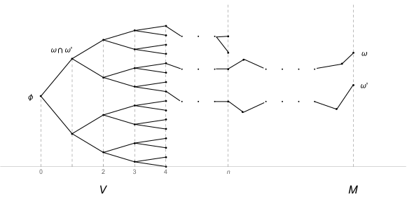
We are concerned with cases of kernels k : D × D → ℝ : 𝑘 → 𝐷 𝐷 ℝ k:D\times D\rightarrow\mathbb{R} k V : V × V → ℝ : subscript 𝑘 𝑉 → 𝑉 𝑉 ℝ k_{V}:V\times V\rightarrow\mathbb{R} V 𝑉 V D 𝐷 D x ∈ V 𝑥 𝑉 x\in V δ x | V ∈ ℋ V evaluated-at subscript 𝛿 𝑥 𝑉 subscript ℋ 𝑉 \delta_{x}\big{|}_{V}\in\mathscr{H}_{V} δ x ∉ ℋ subscript 𝛿 𝑥 ℋ \delta_{x}\notin\mathscr{H} k 𝑘 k
D = ℝ + 𝐷 subscript ℝ D=\mathbb{R}_{+}
V = 𝑉 absent V= 0 < x 1 < x 2 < ⋯ < x i < x i + 1 < ⋯ 0 subscript 𝑥 1 subscript 𝑥 2 ⋯ subscript 𝑥 𝑖 subscript 𝑥 𝑖 1 ⋯ 0<x_{1}<x_{2}<\cdots<x_{i}<x_{i+1}<\cdots V = { x i } i = 1 ∞ 𝑉 superscript subscript subscript 𝑥 𝑖 𝑖 1 V=\left\{x_{i}\right\}_{i=1}^{\infty}
In this case, we compute ℋ V subscript ℋ 𝑉 \mathscr{H}_{V} δ x i | V ∈ ℋ V evaluated-at subscript 𝛿 subscript 𝑥 𝑖 𝑉 subscript ℋ 𝑉 \delta_{x_{i}}\big{|}_{V}\in\mathscr{H}_{V} ℋ m = subscript ℋ 𝑚 absent \mathscr{H}_{m}= δ x i ∉ ℋ m subscript 𝛿 subscript 𝑥 𝑖 subscript ℋ 𝑚 \delta_{x_{i}}\notin\mathscr{H}_{m}
Also note that δ x 1 subscript 𝛿 subscript 𝑥 1 \delta_{x_{1}} ℋ V subscript ℋ 𝑉 \mathscr{H}_{V} ℋ m subscript ℋ 𝑚 \mathscr{H}_{m} δ x 1 ( y ) = { 1 y = x 1 0 y ∈ V \ { x 1 } subscript 𝛿 subscript 𝑥 1 𝑦 cases 1 𝑦 subscript 𝑥 1 0 𝑦 \ 𝑉 subscript 𝑥 1 \delta_{x_{1}}\left(y\right)=\begin{cases}1&y=x_{1}\\
0&y\in V\backslash\left\{x_{1}\right\}\end{cases} δ x 1 subscript 𝛿 subscript 𝑥 1 \delta_{x_{1}} δ x subscript 𝛿 𝑥 \delta_{x}
In the following, we will consider restriction to V × V 𝑉 𝑉 V\times V k 𝑘 k ℝ + × ℝ + subscript ℝ subscript ℝ \mathbb{R}_{+}\times\mathbb{R}_{+} k ( s , t ) = s ∧ t = min ( s , t ) 𝑘 𝑠 𝑡 𝑠 𝑡 𝑠 𝑡 k\left(s,t\right)=s\wedge t=\min\left(s,t\right) k 𝑘 k f 𝑓 f ℝ + subscript ℝ \mathbb{R}_{+} f ′ ∈ L 2 ( ℝ + ) superscript 𝑓 ′ superscript 𝐿 2 subscript ℝ f^{\prime}\in L^{2}\left(\mathbb{R}_{+}\right)
‖ f ‖ ℋ 2 := ∫ 0 ∞ | f ′ ( t ) | 2 𝑑 t < ∞ . assign superscript subscript norm 𝑓 ℋ 2 superscript subscript 0 superscript superscript 𝑓 ′ 𝑡 2 differential-d 𝑡 \left\|f\right\|_{\mathscr{H}}^{2}:=\int_{0}^{\infty}\left|f^{\prime}\left(t\right)\right|^{2}dt<\infty. (3.1)
For details, see below.
Application. The Hilbert space given by ∥ ⋅ ∥ ℋ 2 \left\|\cdot\right\|_{\mathscr{H}}^{2} 3.1 k : ℝ + × ℝ + → ℝ : : 𝑘 → subscript ℝ subscript ℝ ℝ : absent k:\mathbb{R}_{+}\times\mathbb{R}_{+}\rightarrow\mathbb{R}: k ( s , t ) := s ∧ t assign 𝑘 𝑠 𝑡 𝑠 𝑡 k\left(s,t\right):=s\wedge t V ⊂ ℝ + 𝑉 subscript ℝ V\subset\mathbb{R}_{+} 3.1 V × V 𝑉 𝑉 V\times V k ( V ) superscript 𝑘 𝑉 k^{\left(V\right)} ℋ ℋ \mathscr{H}
J ( V ) ( k x ( V ) ) = k x , ∀ x ∈ V ; formulae-sequence superscript 𝐽 𝑉 superscript subscript 𝑘 𝑥 𝑉 subscript 𝑘 𝑥 for-all 𝑥 𝑉 J^{\left(V\right)}\left(k_{x}^{\left(V\right)}\right)=k_{x},\quad\forall x\in V; (3.2)
J ( V ) superscript 𝐽 𝑉 J^{\left(V\right)} ℋ V → J ( V ) ℋ superscript 𝐽 𝑉 → subscript ℋ 𝑉 ℋ \mathscr{H}_{V}\xrightarrow{J^{\left(V\right)}}\mathscr{H} J ( V ) superscript 𝐽 𝑉 J^{\left(V\right)}
Note that P V := J ( V ) ( J ( V ) ) ∗ assign subscript 𝑃 𝑉 superscript 𝐽 𝑉 superscript superscript 𝐽 𝑉 P_{V}:=J^{\left(V\right)}\left(J^{\left(V\right)}\right)^{*} J ( V ) superscript 𝐽 𝑉 J^{\left(V\right)}
ℋ ⊖ ℋ V = { ψ ∈ ℋ | ψ ( x ) = 0 , ∀ x ∈ V } . symmetric-difference ℋ subscript ℋ 𝑉 conditional-set 𝜓 ℋ formulae-sequence 𝜓 𝑥 0 for-all 𝑥 𝑉 \mathscr{H}\ominus\mathscr{H}_{V}=\left\{\psi\in\mathscr{H}\>\big{|}\>\psi\left(x\right)=0,\;\forall x\in V\right\}. (3.3)
Example 3.2 .
Let k 𝑘 k k ( V ) superscript 𝑘 𝑉 k^{\left(V\right)} 3.2 V := π ℤ + assign 𝑉 𝜋 subscript ℤ V:=\pi\mathbb{Z}_{+} π 𝜋 \pi [BJ02 ] ) yield non-zero
functions ψ 𝜓 \psi ℝ + subscript ℝ \mathbb{R}_{+}
ψ ∈ ℋ ⊖ ℋ V . 𝜓 symmetric-difference ℋ subscript ℋ 𝑉 \psi\in\mathscr{H}\ominus\mathscr{H}_{V}. (3.4)
More precisely,
0 < ∫ 0 ∞ | ψ ′ ( t ) | 2 𝑑 t < ∞ , 0 superscript subscript 0 superscript superscript 𝜓 ′ 𝑡 2 differential-d 𝑡 0<\int_{0}^{\infty}\left|\psi^{\prime}\left(t\right)\right|^{2}dt<\infty, (3.5)
where ψ ′ superscript 𝜓 ′ \psi^{\prime}
ψ ( n π ) = 0 , ∀ n ∈ ℤ + . formulae-sequence 𝜓 𝑛 𝜋 0 for-all 𝑛 subscript ℤ \psi\left(n\pi\right)=0,\quad\forall n\in\mathbb{Z}_{+}. (3.6)
An explicit solution to (3.4 3.6
ψ ( t ) = ∏ n = 1 ∞ cos ( t 2 n ) = sin t t , ∀ t ∈ ℝ . formulae-sequence 𝜓 𝑡 superscript subscript product 𝑛 1 𝑡 superscript 2 𝑛 𝑡 𝑡 for-all 𝑡 ℝ \psi\left(t\right)=\prod_{n=1}^{\infty}\cos\left(\frac{t}{2^{n}}\right)=\frac{\sin t}{t},\quad\forall t\in\mathbb{R}. (3.7)
From this, one easily generates an infinite-dimensional set of solutions.
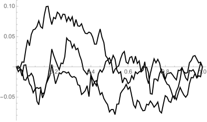
3.1. Brownian motion
Consider the covariance function of standard Brownian motion B t subscript 𝐵 𝑡 B_{t} t ∈ [ 0 , ∞ ) 𝑡 0 t\in[0,\infty) { B t } subscript 𝐵 𝑡 \left\{B_{t}\right\}
𝔼 ( B s B t ) = s ∧ t = min ( s , t ) . 𝔼 subscript 𝐵 𝑠 subscript 𝐵 𝑡 𝑠 𝑡 𝑠 𝑡 \mathbb{E}\left(B_{s}B_{t}\right)=s\wedge t=\min\left(s,t\right). (3.8)
We now show that the restriction of (3.8 V × V 𝑉 𝑉 V\times V V 𝑉 V
V : 0 < x 1 < x 2 < ⋯ < x i < x i + 1 < ⋯ : 𝑉 0 subscript 𝑥 1 subscript 𝑥 2 ⋯ subscript 𝑥 𝑖 subscript 𝑥 𝑖 1 ⋯ V:\;0<x_{1}<x_{2}<\cdots<x_{i}<x_{i+1}<\cdots (3.9)
has the discrete mass property (Def. 2.4
Set ℋ V = R K H S ( k | V × V ) subscript ℋ 𝑉 𝑅 𝐾 𝐻 𝑆 evaluated-at 𝑘 𝑉 𝑉 \mathscr{H}_{V}=RKHS(k\big{|}_{V\times V})
k V ( x i , x j ) = x i ∧ x j . subscript 𝑘 𝑉 subscript 𝑥 𝑖 subscript 𝑥 𝑗 subscript 𝑥 𝑖 subscript 𝑥 𝑗 k_{V}\left(x_{i},x_{j}\right)=x_{i}\wedge x_{j}. (3.10)
We consider the set F n = { x 1 , x 2 , … , x n } subscript 𝐹 𝑛 subscript 𝑥 1 subscript 𝑥 2 … subscript 𝑥 𝑛 F_{n}=\left\{x_{1},x_{2},\ldots,x_{n}\right\} V 𝑉 V
K n = k ( F n ) = [ x 1 x 1 x 1 ⋯ x 1 x 1 x 2 x 2 ⋯ x 2 x 1 x 2 x 3 ⋯ x 3 ⋮ ⋮ ⋮ ⋮ ⋮ x 1 x 2 x 3 ⋯ x n ] = ( x i ∧ x j ) i , j = 1 n . subscript 𝐾 𝑛 superscript 𝑘 subscript 𝐹 𝑛 matrix subscript 𝑥 1 subscript 𝑥 1 subscript 𝑥 1 ⋯ subscript 𝑥 1 subscript 𝑥 1 subscript 𝑥 2 subscript 𝑥 2 ⋯ subscript 𝑥 2 subscript 𝑥 1 subscript 𝑥 2 subscript 𝑥 3 ⋯ subscript 𝑥 3 ⋮ ⋮ ⋮ ⋮ ⋮ subscript 𝑥 1 subscript 𝑥 2 subscript 𝑥 3 ⋯ subscript 𝑥 𝑛 superscript subscript subscript 𝑥 𝑖 subscript 𝑥 𝑗 𝑖 𝑗
1 𝑛 K_{n}=k^{\left(F_{n}\right)}=\begin{bmatrix}x_{1}&x_{1}&x_{1}&\cdots&x_{1}\\
x_{1}&x_{2}&x_{2}&\cdots&x_{2}\\
x_{1}&x_{2}&x_{3}&\cdots&x_{3}\\
\vdots&\vdots&\vdots&\vdots&\vdots\\
x_{1}&x_{2}&x_{3}&\cdots&x_{n}\end{bmatrix}=\left(x_{i}\wedge x_{j}\right)_{i,j=1}^{n}. (3.11)
We will show that condition (iii) 2.12 k V subscript 𝑘 𝑉 k_{V} D n = det ( K F ) subscript 𝐷 𝑛 subscript 𝐾 𝐹 D_{n}=\det\left(K_{F}\right) n = # F 𝑛 # 𝐹 n=\#F 2.20
Lemma 3.3 .
D n = det ( ( x i ∧ x j ) i , j = 1 n ) = x 1 ( x 2 − x 1 ) ( x 3 − x 2 ) ⋯ ( x n − x n − 1 ) . subscript 𝐷 𝑛 superscript subscript subscript 𝑥 𝑖 subscript 𝑥 𝑗 𝑖 𝑗
1 𝑛 subscript 𝑥 1 subscript 𝑥 2 subscript 𝑥 1 subscript 𝑥 3 subscript 𝑥 2 ⋯ subscript 𝑥 𝑛 subscript 𝑥 𝑛 1 D_{n}=\det\left(\left(x_{i}\wedge x_{j}\right)_{i,j=1}^{n}\right)=x_{1}\left(x_{2}-x_{1}\right)\left(x_{3}-x_{2}\right)\cdots\left(x_{n}-x_{n-1}\right). (3.12)
Proof.
Induction. In fact,
[ x 1 x 1 x 1 ⋯ x 1 x 1 x 2 x 2 ⋯ x 2 x 1 x 2 x 3 ⋯ x 3 ⋮ ⋮ ⋮ ⋮ ⋮ x 1 x 2 x 3 ⋯ x n ] ∼ [ x 1 0 0 ⋯ 0 0 x 2 − x 1 0 ⋯ 0 0 0 x 3 − x 2 ⋯ 0 ⋮ ⋮ ⋮ ⋱ ⋮ 0 ⋯ 0 ⋯ x n − x n − 1 ] , similar-to matrix subscript 𝑥 1 subscript 𝑥 1 subscript 𝑥 1 ⋯ subscript 𝑥 1 subscript 𝑥 1 subscript 𝑥 2 subscript 𝑥 2 ⋯ subscript 𝑥 2 subscript 𝑥 1 subscript 𝑥 2 subscript 𝑥 3 ⋯ subscript 𝑥 3 ⋮ ⋮ ⋮ ⋮ ⋮ subscript 𝑥 1 subscript 𝑥 2 subscript 𝑥 3 ⋯ subscript 𝑥 𝑛 matrix subscript 𝑥 1 0 0 ⋯ 0 0 subscript 𝑥 2 subscript 𝑥 1 0 ⋯ 0 0 0 subscript 𝑥 3 subscript 𝑥 2 ⋯ 0 ⋮ ⋮ ⋮ ⋱ ⋮ 0 ⋯ 0 ⋯ subscript 𝑥 𝑛 subscript 𝑥 𝑛 1 \begin{bmatrix}x_{1}&x_{1}&x_{1}&\cdots&x_{1}\\
x_{1}&x_{2}&x_{2}&\cdots&x_{2}\\
x_{1}&x_{2}&x_{3}&\cdots&x_{3}\\
\vdots&\vdots&\vdots&\vdots&\vdots\\
x_{1}&x_{2}&x_{3}&\cdots&x_{n}\end{bmatrix}\sim\begin{bmatrix}x_{1}&0&0&\cdots&0\\
0&x_{2}-x_{1}&0&\cdots&0\\
0&0&x_{3}-x_{2}&\cdots&0\\
\vdots&\vdots&\vdots&\ddots&\vdots\\
0&\cdots&0&\cdots&x_{n}-x_{n-1}\end{bmatrix},
unitary equivalence in finite dimensions.
∎
Lemma 3.4 .
Let
ζ ( n ) := K n − 1 ( δ x 1 ) ( ⋅ ) assign subscript 𝜁 𝑛 superscript subscript 𝐾 𝑛 1 subscript 𝛿 subscript 𝑥 1 ⋅ \zeta_{\left(n\right)}:=K_{n}^{-1}\left(\delta_{x_{1}}\right)\left(\cdot\right) (3.13)
be as in eq. (2.11
‖ P F n ( δ x 1 ) ‖ ℋ V 2 = ζ ( n ) ( x 1 ) . superscript subscript norm subscript 𝑃 subscript 𝐹 𝑛 subscript 𝛿 subscript 𝑥 1 subscript ℋ 𝑉 2 subscript 𝜁 𝑛 subscript 𝑥 1 \left\|P_{F_{n}}\left(\delta_{x_{1}}\right)\right\|_{\mathscr{H}_{V}}^{2}=\zeta_{\left(n\right)}\left(x_{1}\right). (3.14)
Then,
ζ ( 1 ) ( x 1 ) subscript 𝜁 1 subscript 𝑥 1 \displaystyle\zeta_{\left(1\right)}\left(x_{1}\right) = \displaystyle= 1 x 1 1 subscript 𝑥 1 \displaystyle\frac{1}{x_{1}}
ζ ( n ) ( x 1 ) subscript 𝜁 𝑛 subscript 𝑥 1 \displaystyle\zeta_{\left(n\right)}\left(x_{1}\right) = \displaystyle= x 2 x 1 ( x 2 − x 1 ) , for n = 2 , 3 , … , formulae-sequence subscript 𝑥 2 subscript 𝑥 1 subscript 𝑥 2 subscript 𝑥 1 for 𝑛
2 3 …
\displaystyle\frac{x_{2}}{x_{1}\left(x_{2}-x_{1}\right)},\quad\text{for}\;n=2,3,\ldots,
and
‖ δ x 1 ‖ ℋ V 2 = x 2 x 1 ( x 2 − x 1 ) . superscript subscript norm subscript 𝛿 subscript 𝑥 1 subscript ℋ 𝑉 2 subscript 𝑥 2 subscript 𝑥 1 subscript 𝑥 2 subscript 𝑥 1 \left\|\delta_{x_{1}}\right\|_{\mathscr{H}_{V}}^{2}=\frac{x_{2}}{x_{1}\left(x_{2}-x_{1}\right)}.
Proof.
A direct computation shows the ( 1 , 1 ) 1 1 \left(1,1\right) K n − 1 superscript subscript 𝐾 𝑛 1 K_{n}^{-1}
D n − 1 ′ = det ( ( x i ∧ x j ) i , j = 2 n ) = x 2 ( x 3 − x 2 ) ( x 4 − x 3 ) ⋯ ( x n − x n − 1 ) subscript superscript 𝐷 ′ 𝑛 1 superscript subscript subscript 𝑥 𝑖 subscript 𝑥 𝑗 𝑖 𝑗
2 𝑛 subscript 𝑥 2 subscript 𝑥 3 subscript 𝑥 2 subscript 𝑥 4 subscript 𝑥 3 ⋯ subscript 𝑥 𝑛 subscript 𝑥 𝑛 1 D^{\prime}_{n-1}=\det\left(\left(x_{i}\wedge x_{j}\right)_{i,j=2}^{n}\right)=x_{2}\left(x_{3}-x_{2}\right)\left(x_{4}-x_{3}\right)\cdots\left(x_{n}-x_{n-1}\right) (3.15)
and so
ζ ( 1 ) ( x 1 ) subscript 𝜁 1 subscript 𝑥 1 \displaystyle\zeta_{\left(1\right)}\left(x_{1}\right) = \displaystyle= 1 x 1 , and 1 subscript 𝑥 1 and
\displaystyle\frac{1}{x_{1}},\quad\mbox{and}
ζ ( 2 ) ( x 1 ) subscript 𝜁 2 subscript 𝑥 1 \displaystyle\zeta_{\left(2\right)}\left(x_{1}\right) = \displaystyle= x 2 x 1 ( x 2 − x 1 ) subscript 𝑥 2 subscript 𝑥 1 subscript 𝑥 2 subscript 𝑥 1 \displaystyle\frac{x_{2}}{x_{1}\left(x_{2}-x_{1}\right)}
ζ ( 3 ) ( x 1 ) subscript 𝜁 3 subscript 𝑥 1 \displaystyle\zeta_{\left(3\right)}\left(x_{1}\right) = \displaystyle= x 2 ( x 3 − x 2 ) x 1 ( x 2 − x 1 ) ( x 3 − x 2 ) = x 2 x 1 ( x 2 − x 1 ) subscript 𝑥 2 subscript 𝑥 3 subscript 𝑥 2 subscript 𝑥 1 subscript 𝑥 2 subscript 𝑥 1 subscript 𝑥 3 subscript 𝑥 2 subscript 𝑥 2 subscript 𝑥 1 subscript 𝑥 2 subscript 𝑥 1 \displaystyle\frac{x_{2}\left(x_{3}-x_{2}\right)}{x_{1}\left(x_{2}-x_{1}\right)\left(x_{3}-x_{2}\right)}=\frac{x_{2}}{x_{1}\left(x_{2}-x_{1}\right)}
ζ ( 4 ) ( x 1 ) subscript 𝜁 4 subscript 𝑥 1 \displaystyle\zeta_{\left(4\right)}\left(x_{1}\right) = \displaystyle= x 2 ( x 3 − x 2 ) ( x 4 − x 3 ) x 1 ( x 2 − x 1 ) ( x 3 − x 2 ) ( x 4 − x 3 ) = x 2 x 1 ( x 2 − x 1 ) subscript 𝑥 2 subscript 𝑥 3 subscript 𝑥 2 subscript 𝑥 4 subscript 𝑥 3 subscript 𝑥 1 subscript 𝑥 2 subscript 𝑥 1 subscript 𝑥 3 subscript 𝑥 2 subscript 𝑥 4 subscript 𝑥 3 subscript 𝑥 2 subscript 𝑥 1 subscript 𝑥 2 subscript 𝑥 1 \displaystyle\frac{x_{2}\left(x_{3}-x_{2}\right)\left(x_{4}-x_{3}\right)}{x_{1}\left(x_{2}-x_{1}\right)\left(x_{3}-x_{2}\right)\left(x_{4}-x_{3}\right)}=\frac{x_{2}}{x_{1}\left(x_{2}-x_{1}\right)}
⋮ ⋮ \displaystyle\vdots
The result follows from this, and from Corollary 2.9
Corollary 3.5 .
P F n ( δ x 1 ) = P F 2 ( δ x 1 ) subscript 𝑃 subscript 𝐹 𝑛 subscript 𝛿 subscript 𝑥 1 subscript 𝑃 subscript 𝐹 2 subscript 𝛿 subscript 𝑥 1 P_{F_{n}}\left(\delta_{x_{1}}\right)=P_{F_{2}}\left(\delta_{x_{1}}\right) ,
∀ n ≥ 2 for-all 𝑛 2 \forall n\geq 2
δ x 1 ∈ ℋ V ( F 2 ) := s p a n { k x 1 ( V ) , k x 2 ( V ) } subscript 𝛿 subscript 𝑥 1 superscript subscript ℋ 𝑉 subscript 𝐹 2 assign 𝑠 𝑝 𝑎 𝑛 superscript subscript 𝑘 subscript 𝑥 1 𝑉 superscript subscript 𝑘 subscript 𝑥 2 𝑉 \delta_{x_{1}}\in\mathscr{H}_{V}^{\left(F_{2}\right)}:=span\{k_{x_{1}}^{\left(V\right)},k_{x_{2}}^{\left(V\right)}\} (3.16)
and
δ x 1 = ζ ( 2 ) ( x 1 ) k x 1 ( V ) + ζ ( 2 ) ( x 2 ) k x 2 ( V ) subscript 𝛿 subscript 𝑥 1 subscript 𝜁 2 subscript 𝑥 1 superscript subscript 𝑘 subscript 𝑥 1 𝑉 subscript 𝜁 2 subscript 𝑥 2 superscript subscript 𝑘 subscript 𝑥 2 𝑉 \delta_{x_{1}}=\zeta_{\left(2\right)}\left(x_{1}\right)k_{x_{1}}^{\left(V\right)}+\zeta_{\left(2\right)}\left(x_{2}\right)k_{x_{2}}^{\left(V\right)} (3.17)
where
ζ ( 2 ) ( x i ) = K 2 − 1 ( δ x 1 ) ( x i ) , i = 1 , 2 . formulae-sequence subscript 𝜁 2 subscript 𝑥 𝑖 superscript subscript 𝐾 2 1 subscript 𝛿 subscript 𝑥 1 subscript 𝑥 𝑖 𝑖 1 2
\zeta_{\left(2\right)}\left(x_{i}\right)=K_{2}^{-1}\left(\delta_{x_{1}}\right)\left(x_{i}\right),\;i=1,2.
Specifically,
ζ ( 2 ) ( x 1 ) subscript 𝜁 2 subscript 𝑥 1 \displaystyle\zeta_{\left(2\right)}\left(x_{1}\right) = \displaystyle= x 2 x 1 ( x 2 − x 1 ) subscript 𝑥 2 subscript 𝑥 1 subscript 𝑥 2 subscript 𝑥 1 \displaystyle\frac{x_{2}}{x_{1}\left(x_{2}-x_{1}\right)} (3.18)
ζ ( 2 ) ( x 2 ) subscript 𝜁 2 subscript 𝑥 2 \displaystyle\zeta_{\left(2\right)}\left(x_{2}\right) = \displaystyle= − 1 x 2 − x 1 ; 1 subscript 𝑥 2 subscript 𝑥 1 \displaystyle\frac{-1}{x_{2}-x_{1}}; (3.19)
and
‖ δ x 1 ‖ ℋ V 2 = x 2 x 1 ( x 2 − x 1 ) . superscript subscript norm subscript 𝛿 subscript 𝑥 1 subscript ℋ 𝑉 2 subscript 𝑥 2 subscript 𝑥 1 subscript 𝑥 2 subscript 𝑥 1 \left\|\delta_{x_{1}}\right\|_{\mathscr{H}_{V}}^{2}=\frac{x_{2}}{x_{1}\left(x_{2}-x_{1}\right)}. (3.20)
Proof.
Follows from the lemma. Note that
ζ n ( x 1 ) = ‖ P F n ( δ x 1 ) ‖ ℋ 2 subscript 𝜁 𝑛 subscript 𝑥 1 superscript subscript norm subscript 𝑃 subscript 𝐹 𝑛 subscript 𝛿 subscript 𝑥 1 ℋ 2 \zeta_{n}\left(x_{1}\right)=\left\|P_{F_{n}}\left(\delta_{x_{1}}\right)\right\|_{\mathscr{H}}^{2}
and ζ ( 1 ) ( x 1 ) ≤ ζ ( 2 ) ( x 1 ) ≤ ⋯ subscript 𝜁 1 subscript 𝑥 1 subscript 𝜁 2 subscript 𝑥 1 ⋯ \zeta_{\left(1\right)}\left(x_{1}\right)\leq\zeta_{\left(2\right)}\left(x_{1}\right)\leq\cdots F n = { x 1 , x 2 , … , x n } subscript 𝐹 𝑛 subscript 𝑥 1 subscript 𝑥 2 … subscript 𝑥 𝑛 F_{n}=\left\{x_{1},x_{2},\ldots,x_{n}\right\} 1 x 1 ≤ x 2 x 1 ( x 2 − x 1 ) 1 subscript 𝑥 1 subscript 𝑥 2 subscript 𝑥 1 subscript 𝑥 2 subscript 𝑥 1 \frac{1}{x_{1}}\leq\frac{x_{2}}{x_{1}\left(x_{2}-x_{1}\right)} 3.20
Remark 3.6 .
We showed that δ x 1 ∈ ℋ V subscript 𝛿 subscript 𝑥 1 subscript ℋ 𝑉 \delta_{x_{1}}\in\mathscr{H}_{V} V = { x 1 < x 2 < ⋯ } ⊂ ℝ + 𝑉 subscript 𝑥 1 subscript 𝑥 2 ⋯ subscript ℝ V=\left\{x_{1}<x_{2}<\cdots\right\}\subset\mathbb{R}_{+} s ∧ t 𝑠 𝑡 s\wedge t
The same argument also shows that δ x i ∈ ℋ V subscript 𝛿 subscript 𝑥 𝑖 subscript ℋ 𝑉 \delta_{x_{i}}\in\mathscr{H}_{V} i > 1 𝑖 1 i>1 δ x 1 ∈ ℋ V subscript 𝛿 subscript 𝑥 1 subscript ℋ 𝑉 \delta_{x_{1}}\in\mathscr{H}_{V}
Fix V = { x i } i = 1 ∞ 𝑉 superscript subscript subscript 𝑥 𝑖 𝑖 1 V=\left\{x_{i}\right\}_{i=1}^{\infty} x 1 < x 2 < ⋯ subscript 𝑥 1 subscript 𝑥 2 ⋯ x_{1}<x_{2}<\cdots
P F n ( δ x i ) = { 0 if n < i − 1 ∑ s = 1 n ( K F n − 1 δ x i ) ( x s ) k x s if n ≥ i subscript 𝑃 subscript 𝐹 𝑛 subscript 𝛿 subscript 𝑥 𝑖 cases 0 if n < i − 1 superscript subscript 𝑠 1 𝑛 superscript subscript 𝐾 subscript 𝐹 𝑛 1 subscript 𝛿 subscript 𝑥 𝑖 subscript 𝑥 𝑠 subscript 𝑘 subscript 𝑥 𝑠 if n ≥ i P_{F_{n}}\left(\delta_{x_{i}}\right)=\begin{cases}0&\text{if $n<i-1$}\\
\sum_{s=1}^{n}\left(K_{F_{n}}^{-1}\delta_{x_{i}}\right)\left(x_{s}\right)k_{x_{s}}&\text{if $n\geq i$}\end{cases}
and
‖ P F n ( δ x i ) ‖ ℋ 2 = { 0 if n < i − 1 1 x i − x i − 1 if n = i x i + 1 − x i − 1 ( x i − x i − 1 ) ( x i + 1 − x i ) if n > i superscript subscript norm subscript 𝑃 subscript 𝐹 𝑛 subscript 𝛿 subscript 𝑥 𝑖 ℋ 2 cases 0 if n < i − 1 1 subscript 𝑥 𝑖 subscript 𝑥 𝑖 1 if n = i subscript 𝑥 𝑖 1 subscript 𝑥 𝑖 1 subscript 𝑥 𝑖 subscript 𝑥 𝑖 1 subscript 𝑥 𝑖 1 subscript 𝑥 𝑖 if n > i \left\|P_{F_{n}}\left(\delta_{x_{i}}\right)\right\|_{\mathscr{H}}^{2}=\begin{cases}0&\text{if $n<i-1$}\\
\frac{1}{x_{i}-x_{i-1}}&\text{if $n=i$}\\
\frac{x_{i+1}-x_{i-1}}{\left(x_{i}-x_{i-1}\right)\left(x_{i+1}-x_{i}\right)}&\text{if $n>i$}\end{cases}
Conclusion.
δ x i subscript 𝛿 subscript 𝑥 𝑖 \displaystyle\delta_{x_{i}} ∈ \displaystyle\in s p a n { k x i − 1 ( V ) , k x i ( V ) , k x i + 1 ( V ) } , and 𝑠 𝑝 𝑎 𝑛 superscript subscript 𝑘 subscript 𝑥 𝑖 1 𝑉 superscript subscript 𝑘 subscript 𝑥 𝑖 𝑉 superscript subscript 𝑘 subscript 𝑥 𝑖 1 𝑉 and
\displaystyle span\left\{k_{x_{i-1}}^{\left(V\right)},k_{x_{i}}^{\left(V\right)},k_{x_{i+1}}^{\left(V\right)}\right\},\quad\mbox{and} (3.21)
‖ δ x i ‖ ℋ 2 superscript subscript norm subscript 𝛿 subscript 𝑥 𝑖 ℋ 2 \displaystyle\left\|\delta_{x_{i}}\right\|_{\mathscr{H}}^{2} = \displaystyle= x i + 1 − x i − 1 ( x i − x i − 1 ) ( x i + 1 − x i ) . subscript 𝑥 𝑖 1 subscript 𝑥 𝑖 1 subscript 𝑥 𝑖 subscript 𝑥 𝑖 1 subscript 𝑥 𝑖 1 subscript 𝑥 𝑖 \displaystyle\frac{x_{i+1}-x_{i-1}}{\left(x_{i}-x_{i-1}\right)\left(x_{i+1}-x_{i}\right)}. (3.22)
Corollary 3.7 .
Let V ⊂ ℝ + 𝑉 subscript ℝ V\subset\mathbb{R}_{+} x a ∈ V subscript 𝑥 𝑎 𝑉 x_{a}\in V V 𝑉 V ‖ δ a ‖ ℋ V = ∞ subscript norm subscript 𝛿 𝑎 subscript ℋ 𝑉 \left\|\delta_{a}\right\|_{\mathscr{H}_{V}}=\infty
Remark 3.8 .
This computation will be revisited in sect. 4
Example 3.9 .
An illustration for 0 < x 1 < x 2 < x 3 < x 4 0 subscript 𝑥 1 subscript 𝑥 2 subscript 𝑥 3 subscript 𝑥 4 0<x_{1}<x_{2}<x_{3}<x_{4}
P F ( δ x 3 ) subscript 𝑃 𝐹 subscript 𝛿 subscript 𝑥 3 \displaystyle P_{F}\left(\delta_{x_{3}}\right) = \displaystyle= ∑ y ∈ F ζ ( F ) ( y ) k y ( ⋅ ) subscript 𝑦 𝐹 superscript 𝜁 𝐹 𝑦 subscript 𝑘 𝑦 ⋅ \displaystyle\sum_{y\in F}\zeta^{\left(F\right)}\left(y\right)k_{y}\left(\cdot\right)
ζ ( F ) superscript 𝜁 𝐹 \displaystyle\zeta^{\left(F\right)} = \displaystyle= K F − 1 δ x 3 . superscript subscript 𝐾 𝐹 1 subscript 𝛿 subscript 𝑥 3 \displaystyle K_{F}^{-1}\delta_{x_{3}}\;.
That is,
[ x 1 x 1 x 1 x 1 x 1 x 2 x 2 x 2 x 1 x 2 x 3 x 3 x 1 x 2 x 3 x 4 ] ⏟ ( K F ( x i , x j ) ) i , j = 1 4 [ ζ ( F ) ( x 1 ) ζ ( F ) ( x 2 ) ζ ( F ) ( x 3 ) ζ ( F ) ( x 4 ) ] = [ 0 0 1 0 ] superscript subscript subscript 𝐾 𝐹 subscript 𝑥 𝑖 subscript 𝑥 𝑗 𝑖 𝑗
1 4 ⏟ matrix subscript 𝑥 1 subscript 𝑥 1 subscript 𝑥 1 subscript 𝑥 1 subscript 𝑥 1 subscript 𝑥 2 subscript 𝑥 2 subscript 𝑥 2 subscript 𝑥 1 subscript 𝑥 2 subscript 𝑥 3 subscript 𝑥 3 subscript 𝑥 1 subscript 𝑥 2 subscript 𝑥 3 subscript 𝑥 4 matrix superscript 𝜁 𝐹 subscript 𝑥 1 superscript 𝜁 𝐹 subscript 𝑥 2 superscript 𝜁 𝐹 subscript 𝑥 3 superscript 𝜁 𝐹 subscript 𝑥 4 matrix 0 0 1 0 \underset{\left(K_{F}\left(x_{i},x_{j}\right)\right)_{i,j=1}^{4}}{\underbrace{\begin{bmatrix}x_{1}&x_{1}&x_{1}&x_{1}\\
x_{1}&x_{2}&x_{2}&x_{2}\\
x_{1}&x_{2}&x_{3}&x_{3}\\
x_{1}&x_{2}&x_{3}&x_{4}\end{bmatrix}}}\begin{bmatrix}\zeta^{\left(F\right)}\left(x_{1}\right)\\
\zeta^{\left(F\right)}\left(x_{2}\right)\\
\zeta^{\left(F\right)}\left(x_{3}\right)\\
\zeta^{\left(F\right)}\left(x_{4}\right)\end{bmatrix}=\begin{bmatrix}0\\
0\\
1\\
0\end{bmatrix}
and
ζ ( F ) ( x 3 ) superscript 𝜁 𝐹 subscript 𝑥 3 \displaystyle\zeta^{\left(F\right)}\left(x_{3}\right) = \displaystyle= x 1 ( x 2 − x 1 ) ( x 4 − x 2 ) x 1 ( x 2 − x 1 ) ( x 3 − x 2 ) ( x 4 − x 3 ) subscript 𝑥 1 subscript 𝑥 2 subscript 𝑥 1 subscript 𝑥 4 subscript 𝑥 2 subscript 𝑥 1 subscript 𝑥 2 subscript 𝑥 1 subscript 𝑥 3 subscript 𝑥 2 subscript 𝑥 4 subscript 𝑥 3 \displaystyle\frac{x_{1}\left(x_{2}-x_{1}\right)\left(x_{4}-x_{2}\right)}{x_{1}\left(x_{2}-x_{1}\right)\left(x_{3}-x_{2}\right)\left(x_{4}-x_{3}\right)}
= \displaystyle= x 4 − x 2 ( x 3 − x 2 ) ( x 4 − x 3 ) = ‖ δ x 3 ‖ ℋ 2 . subscript 𝑥 4 subscript 𝑥 2 subscript 𝑥 3 subscript 𝑥 2 subscript 𝑥 4 subscript 𝑥 3 superscript subscript norm subscript 𝛿 subscript 𝑥 3 ℋ 2 \displaystyle\frac{x_{4}-x_{2}}{\left(x_{3}-x_{2}\right)\left(x_{4}-x_{3}\right)}=\left\|\delta_{x_{3}}\right\|_{\mathscr{H}}^{2}.
Example 3.10 (Sparse sample-points).
Let V = { x i } i = 1 ∞ 𝑉 superscript subscript subscript 𝑥 𝑖 𝑖 1 V=\left\{x_{i}\right\}_{i=1}^{\infty}
x i = i ( i − 1 ) 2 , i ∈ ℕ . formulae-sequence subscript 𝑥 𝑖 𝑖 𝑖 1 2 𝑖 ℕ x_{i}=\frac{i\left(i-1\right)}{2},\quad i\in\mathbb{N}.
It follows that x i + 1 − x i = i subscript 𝑥 𝑖 1 subscript 𝑥 𝑖 𝑖 x_{i+1}-x_{i}=i
‖ δ x i ‖ ℋ 2 = x i + 1 − x i ( x i − x i − 1 ) ( x i + 1 − x i ) = 2 i − 1 ( i − 1 ) i → i → ∞ 0 . superscript subscript norm subscript 𝛿 subscript 𝑥 𝑖 ℋ 2 subscript 𝑥 𝑖 1 subscript 𝑥 𝑖 subscript 𝑥 𝑖 subscript 𝑥 𝑖 1 subscript 𝑥 𝑖 1 subscript 𝑥 𝑖 2 𝑖 1 𝑖 1 𝑖 → 𝑖 absent → 0 \left\|\delta_{x_{i}}\right\|_{\mathscr{H}}^{2}=\frac{x_{i+1}-x_{i}}{\left(x_{i}-x_{i-1}\right)\left(x_{i+1}-x_{i}\right)}=\frac{2i-1}{\left(i-1\right)i}\xrightarrow[i\rightarrow\infty]{}0.
Conclusion. ‖ δ x i ‖ ℋ → i → ∞ 0 → 𝑖 absent → subscript norm subscript 𝛿 subscript 𝑥 𝑖 ℋ 0 \left\|\delta_{x_{i}}\right\|_{\mathscr{H}}\xrightarrow[i\rightarrow\infty]{}0 V = { x i } i = 1 ∞ ⊂ ℝ + 𝑉 superscript subscript subscript 𝑥 𝑖 𝑖 1 subscript ℝ V=\left\{x_{i}\right\}_{i=1}^{\infty}\subset\mathbb{R}_{+}
Lemma 3.11 .
Let k : V × V → ℂ : 𝑘 → 𝑉 𝑉 ℂ k:V\times V\rightarrow\mathbb{C} ℋ ℋ \mathscr{H} x 1 ∈ V subscript 𝑥 1 𝑉 x_{1}\in V δ x 1 subscript 𝛿 subscript 𝑥 1 \delta_{x_{1}}
δ x 1 = ∑ y ∈ V ζ ( x 1 ) ( y ) k y , subscript 𝛿 subscript 𝑥 1 subscript 𝑦 𝑉 superscript 𝜁 subscript 𝑥 1 𝑦 subscript 𝑘 𝑦 \delta_{x_{1}}=\sum_{y\in V}\zeta^{\left(x_{1}\right)}\left(y\right)k_{y}\;, (3.23)
then
‖ δ x 1 ‖ ℋ 2 = ζ ( x 1 ) ( x 1 ) . superscript subscript norm subscript 𝛿 subscript 𝑥 1 ℋ 2 superscript 𝜁 subscript 𝑥 1 subscript 𝑥 1 \left\|\delta_{x_{1}}\right\|_{\mathscr{H}}^{2}=\zeta^{\left(x_{1}\right)}\left(x_{1}\right). (3.24)
Proof.
Substitute both sides of (3.23 ⟨ δ x 1 , ⋅ ⟩ ℋ subscript subscript 𝛿 subscript 𝑥 1 ⋅
ℋ \left\langle\delta_{x_{1}},\cdot\right\rangle_{\mathscr{H}} ⟨ ⋅ , ⋅ ⟩ ℋ subscript ⋅ ⋅
ℋ \left\langle\cdot,\cdot\right\rangle_{\mathscr{H}} ℋ ℋ \mathscr{H}
Application. Suppose V = ∪ n F n 𝑉 subscript 𝑛 subscript 𝐹 𝑛 V=\cup_{n}F_{n} F n ⊂ F n + 1 subscript 𝐹 𝑛 subscript 𝐹 𝑛 1 F_{n}\subset F_{n+1} F n ∈ ℱ ( V ) subscript 𝐹 𝑛 ℱ 𝑉 F_{n}\in\mathscr{F}\left(V\right) x 1 ∈ F n subscript 𝑥 1 subscript 𝐹 𝑛 x_{1}\in F_{n}
P F n ( δ x 1 ) = ∑ y ∈ F n ⟨ x 1 , K F n − 1 y ⟩ l 2 k y subscript 𝑃 subscript 𝐹 𝑛 subscript 𝛿 subscript 𝑥 1 subscript 𝑦 subscript 𝐹 𝑛 subscript subscript 𝑥 1 superscript subscript 𝐾 subscript 𝐹 𝑛 1 𝑦
superscript 𝑙 2 subscript 𝑘 𝑦 P_{F_{n}}\left(\delta_{x_{1}}\right)=\sum_{y\in F_{n}}\left\langle x_{1},K_{F_{n}}^{-1}y\right\rangle_{l^{2}}k_{y} (3.25)
and
‖ P F n ( δ x 1 ) ‖ ℋ 2 = ⟨ x 1 , K F n − 1 x 1 ⟩ l 2 = ( K F n − 1 δ x 1 ) ( x 1 ) superscript subscript norm subscript 𝑃 subscript 𝐹 𝑛 subscript 𝛿 subscript 𝑥 1 ℋ 2 subscript subscript 𝑥 1 superscript subscript 𝐾 subscript 𝐹 𝑛 1 subscript 𝑥 1
superscript 𝑙 2 superscript subscript 𝐾 subscript 𝐹 𝑛 1 subscript 𝛿 subscript 𝑥 1 subscript 𝑥 1 \left\|P_{F_{n}}\left(\delta_{x_{1}}\right)\right\|_{\mathscr{H}}^{2}=\left\langle x_{1},K_{F_{n}}^{-1}x_{1}\right\rangle_{l^{2}}=\left(K_{F_{n}}^{-1}\delta_{x_{1}}\right)\left(x_{1}\right) (3.26)
and the expression ‖ P F n ( δ x 1 ) ‖ ℋ 2 superscript subscript norm subscript 𝑃 subscript 𝐹 𝑛 subscript 𝛿 subscript 𝑥 1 ℋ 2 \left\|P_{F_{n}}\left(\delta_{x_{1}}\right)\right\|_{\mathscr{H}}^{2} n 𝑛 n
‖ P F n ( δ x 1 ) ‖ ℋ 2 ≤ ‖ P F n + 1 ( δ x 1 ) ‖ ℋ 2 ≤ ⋯ ≤ ‖ δ x 1 ‖ ℋ superscript subscript norm subscript 𝑃 subscript 𝐹 𝑛 subscript 𝛿 subscript 𝑥 1 ℋ 2 superscript subscript norm subscript 𝑃 subscript 𝐹 𝑛 1 subscript 𝛿 subscript 𝑥 1 ℋ 2 ⋯ subscript norm subscript 𝛿 subscript 𝑥 1 ℋ \left\|P_{F_{n}}\left(\delta_{x_{1}}\right)\right\|_{\mathscr{H}}^{2}\leq\left\|P_{F_{n+1}}\left(\delta_{x_{1}}\right)\right\|_{\mathscr{H}}^{2}\leq\cdots\leq\left\|\delta_{x_{1}}\right\|_{\mathscr{H}}
with
sup n ∈ ℕ ‖ P F n ( δ x 1 ) ‖ ℋ 2 = lim n → ∞ ‖ P F n ( δ x 1 ) ‖ ℋ 2 = ‖ δ x 1 ‖ ℋ . subscript supremum 𝑛 ℕ superscript subscript norm subscript 𝑃 subscript 𝐹 𝑛 subscript 𝛿 subscript 𝑥 1 ℋ 2 subscript → 𝑛 superscript subscript norm subscript 𝑃 subscript 𝐹 𝑛 subscript 𝛿 subscript 𝑥 1 ℋ 2 subscript norm subscript 𝛿 subscript 𝑥 1 ℋ \sup_{n\in\mathbb{N}}\left\|P_{F_{n}}\left(\delta_{x_{1}}\right)\right\|_{\mathscr{H}}^{2}=\lim_{n\rightarrow\infty}\left\|P_{F_{n}}\left(\delta_{x_{1}}\right)\right\|_{\mathscr{H}}^{2}=\left\|\delta_{x_{1}}\right\|_{\mathscr{H}}.
Question 3.12 .
Let k : ℝ d × ℝ d → ℝ : 𝑘 → superscript ℝ 𝑑 superscript ℝ 𝑑 ℝ k:\mathbb{R}^{d}\times\mathbb{R}^{d}\rightarrow\mathbb{R} V ⊂ ℝ d 𝑉 superscript ℝ 𝑑 V\subset\mathbb{R}^{d} V = ℤ d 𝑉 superscript ℤ 𝑑 V=\mathbb{Z}^{d} k | V × V evaluated-at 𝑘 𝑉 𝑉 k\big{|}_{V\times V} discrete mass property?
Examples of the affirmative, or not, will be discussed below.
3.2. Discrete RKHS from restrictions
Let D := [ 0 , ∞ ) assign 𝐷 0 D:=[0,\infty) k : D × D → ℝ : 𝑘 → 𝐷 𝐷 ℝ k:D\times D\rightarrow\mathbb{R}
k ( x , y ) = x ∧ y = min ( x , y ) . 𝑘 𝑥 𝑦 𝑥 𝑦 𝑥 𝑦 k\left(x,y\right)=x\wedge y=\min\left(x,y\right).
Restrict to V := { 0 } ∪ ℤ + ⊂ D assign 𝑉 0 subscript ℤ 𝐷 V:=\left\{0\right\}\cup\mathbb{Z}_{+}\subset D
k ( V ) = k | V × V . superscript 𝑘 𝑉 evaluated-at 𝑘 𝑉 𝑉 k^{\left(V\right)}=k\big{|}_{V\times V}.
ℋ ( k ) ℋ 𝑘 \mathscr{H}\left(k\right) f ∈ L 2 ( ℝ ) 𝑓 superscript 𝐿 2 ℝ f\in L^{2}\left(\mathbb{R}\right)
∫ 0 ∞ | f ′ ( x ) | 2 𝑑 x < ∞ , f ( 0 ) = 0 . formulae-sequence superscript subscript 0 superscript superscript 𝑓 ′ 𝑥 2 differential-d 𝑥 𝑓 0 0 \int_{0}^{\infty}\left|f^{\prime}\left(x\right)\right|^{2}dx<\infty,\quad f\left(0\right)=0.
ℋ V := ℋ ( k V ) assign subscript ℋ 𝑉 ℋ subscript 𝑘 𝑉 \mathscr{H}_{V}:=\mathscr{H}\left(k_{V}\right)
f ∈ ℋ ( k V ) ⟺ ∑ n | f ( n ) − f ( n + 1 ) | 2 < ∞ . ⟺ 𝑓 ℋ subscript 𝑘 𝑉 subscript 𝑛 superscript 𝑓 𝑛 𝑓 𝑛 1 2 f\in\mathscr{H}\left(k_{V}\right)\Longleftrightarrow\sum_{n}\left|f\left(n\right)-f\left(n+1\right)\right|^{2}<\infty.
Lemma 3.13 .
We have δ n = 2 k n − k n + 1 − k n − 1 subscript 𝛿 𝑛 2 subscript 𝑘 𝑛 subscript 𝑘 𝑛 1 subscript 𝑘 𝑛 1 \delta_{n}=2k_{n}-k_{n+1}-k_{n-1}
Proof.
Introduce the discrete Laplacian Δ Δ \Delta
( Δ f ) ( n ) = 2 f ( n ) − f ( n − 1 ) − f ( n + 1 ) , Δ 𝑓 𝑛 2 𝑓 𝑛 𝑓 𝑛 1 𝑓 𝑛 1 \left(\Delta f\right)\left(n\right)=2f\left(n\right)-f\left(n-1\right)-f\left(n+1\right),
then Δ k n = δ n Δ subscript 𝑘 𝑛 subscript 𝛿 𝑛 \Delta k_{n}=\delta_{n}
⟨ 2 k n − k n + 1 − k n − 1 , k m ⟩ ℋ V = ⟨ δ n , k m ⟩ ℋ V = δ n , m . subscript 2 subscript 𝑘 𝑛 subscript 𝑘 𝑛 1 subscript 𝑘 𝑛 1 subscript 𝑘 𝑚
subscript ℋ 𝑉 subscript subscript 𝛿 𝑛 subscript 𝑘 𝑚
subscript ℋ 𝑉 subscript 𝛿 𝑛 𝑚
\left\langle 2k_{n}-k_{n+1}-k_{n-1},k_{m}\right\rangle_{\mathscr{H}_{V}}=\left\langle\delta_{n},k_{m}\right\rangle_{\mathscr{H}_{V}}=\delta_{n,m}.
∎
Remark 3.14 .
The same argument as in the proof of the lemma shows (mutatis
mutandis ) that any ordered discrete countable infinite subset V ⊂ [ 0 , ∞ ) 𝑉 0 V\subset[0,\infty)
ℋ V := ℋ ( k | V × V ) assign subscript ℋ 𝑉 ℋ evaluated-at 𝑘 𝑉 𝑉 \mathscr{H}_{V}:=\mathscr{H}\left(k\big{|}_{V\times V}\right)
as a RKHS which is discrete in that (Def. 2.4 V = { x i } i = 1 ∞ 𝑉 superscript subscript subscript 𝑥 𝑖 𝑖 1 V=\left\{x_{i}\right\}_{i=1}^{\infty} x i ∈ ℝ + subscript 𝑥 𝑖 subscript ℝ x_{i}\in\mathbb{R}_{+} δ x i ∈ ℋ V subscript 𝛿 subscript 𝑥 𝑖 subscript ℋ 𝑉 \delta_{x_{i}}\in\mathscr{H}_{V} ∀ i ∈ ℕ for-all 𝑖 ℕ \forall i\in\mathbb{N}
Proof.
Fix vertices V = { x i } i = 1 ∞ 𝑉 superscript subscript subscript 𝑥 𝑖 𝑖 1 V=\left\{x_{i}\right\}_{i=1}^{\infty}
0 < x 1 < x 2 < ⋯ < x i < x i + 1 < ∞ , x i → ∞ . formulae-sequence 0 subscript 𝑥 1 subscript 𝑥 2 ⋯ subscript 𝑥 𝑖 subscript 𝑥 𝑖 1 → subscript 𝑥 𝑖 0<x_{1}<x_{2}<\cdots<x_{i}<x_{i+1}<\infty,\quad x_{i}\rightarrow\infty. (3.27)
Assign conductance
c i , i + 1 = c i + 1 , i = 1 x i + 1 − x i ( = 1 dist ) subscript 𝑐 𝑖 𝑖 1
subscript 𝑐 𝑖 1 𝑖
annotated 1 subscript 𝑥 𝑖 1 subscript 𝑥 𝑖 absent 1 dist c_{i,i+1}=c_{i+1,i}=\frac{1}{x_{i+1}-x_{i}}\left(=\frac{1}{\text{dist}}\right) (3.28)
Let
( Δ f ) ( x i ) Δ 𝑓 subscript 𝑥 𝑖 \displaystyle\left(\Delta f\right)\left(x_{i}\right) = \displaystyle= ( 1 x i + 1 − x i + 1 x i − x i − 1 ) f ( x i ) 1 subscript 𝑥 𝑖 1 subscript 𝑥 𝑖 1 subscript 𝑥 𝑖 subscript 𝑥 𝑖 1 𝑓 subscript 𝑥 𝑖 \displaystyle\left(\frac{1}{x_{i+1}-x_{i}}+\frac{1}{x_{i}-x_{i-1}}\right)f\left(x_{i}\right) (3.29)
− 1 x i − x i − 1 f ( x i − 1 ) − 1 x i + 1 − x i f ( x i + 1 ) 1 subscript 𝑥 𝑖 subscript 𝑥 𝑖 1 𝑓 subscript 𝑥 𝑖 1 1 subscript 𝑥 𝑖 1 subscript 𝑥 𝑖 𝑓 subscript 𝑥 𝑖 1 \displaystyle-\frac{1}{x_{i}-x_{i-1}}f\left(x_{i-1}\right)-\frac{1}{x_{i+1}-x_{i}}f\left(x_{i+1}\right)
Equivalently,
( Δ f ) ( x i ) = ( c i , i + 1 + c i , i − 1 ) f ( x i ) − c i , i − 1 f ( x i − 1 ) − c i , i + 1 f ( x i + 1 ) . Δ 𝑓 subscript 𝑥 𝑖 subscript 𝑐 𝑖 𝑖 1
subscript 𝑐 𝑖 𝑖 1
𝑓 subscript 𝑥 𝑖 subscript 𝑐 𝑖 𝑖 1
𝑓 subscript 𝑥 𝑖 1 subscript 𝑐 𝑖 𝑖 1
𝑓 subscript 𝑥 𝑖 1 \left(\Delta f\right)\left(x_{i}\right)=\left(c_{i,i+1}+c_{i,i-1}\right)f\left(x_{i}\right)-c_{i,i-1}f\left(x_{i-1}\right)-c_{i,i+1}f\left(x_{i+1}\right). (3.30)
Remark 3.15 .
The most general graph-Laplacians will be discussed in detail in sect.
4
Then, with (3.30
Δ k x i = δ x i Δ subscript 𝑘 subscript 𝑥 𝑖 subscript 𝛿 subscript 𝑥 𝑖 \Delta k_{x_{i}}=\delta_{x_{i}}
where k ( ⋅ , ⋅ ) = 𝑘 ⋅ ⋅ absent k\left(\cdot,\cdot\right)= s ∧ t 𝑠 𝑡 s\wedge t [ 0 , ∞ ) × [ 0 , ∞ ) 0 0 [0,\infty)\times[0,\infty) V × V 𝑉 𝑉 V\times V
δ x i = ( c i , i + 1 + c i , i − 1 ) k x i − c i , i + 1 k x i + 1 − c i , i − 1 k x i − 1 ∈ ℋ V subscript 𝛿 subscript 𝑥 𝑖 subscript 𝑐 𝑖 𝑖 1
subscript 𝑐 𝑖 𝑖 1
subscript 𝑘 subscript 𝑥 𝑖 subscript 𝑐 𝑖 𝑖 1
subscript 𝑘 subscript 𝑥 𝑖 1 subscript 𝑐 𝑖 𝑖 1
subscript 𝑘 subscript 𝑥 𝑖 1 subscript ℋ 𝑉 \delta_{x_{i}}=\left(c_{i,i+1}+c_{i,i-1}\right)k_{x_{i}}-c_{i,i+1}k_{x_{i+1}}-c_{i,i-1}k_{x_{i-1}}\in\mathscr{H}_{V} (3.31)
as the RHS in the last equation is a finite sum. Note that now the
RKHS is
ℋ V = { f : V → ℂ | ∑ i = 1 ∞ c i , i + 1 | f ( x i + 1 ) − f ( x i ) | 2 < ∞ } . \mathscr{H}_{V}=\left\{f:V\rightarrow\mathbb{C}\>\big{|}\>\sum_{i=1}^{\infty}c_{i,i+1}\left|f\left(x_{i+1}\right)-f\left(x_{i}\right)\right|^{2}<\infty\right\}.
3.3. The Brownian bridge
Let D := ( 0 , 1 ) = assign 𝐷 0 1 absent D:=\left(0,1\right)= 0 < t < 1 0 𝑡 1 0<t<1
k b r i d g e ( s , t ) := s ∧ t − s t ; assign subscript 𝑘 𝑏 𝑟 𝑖 𝑑 𝑔 𝑒 𝑠 𝑡 𝑠 𝑡 𝑠 𝑡 k_{bridge}\left(s,t\right):=s\wedge t-st; (3.32)
then (3.32 B b r i ( t ) subscript 𝐵 𝑏 𝑟 𝑖 𝑡 B_{bri}\left(t\right)
B b r i ( 0 ) = B b r i ( 1 ) = 0 subscript 𝐵 𝑏 𝑟 𝑖 0 subscript 𝐵 𝑏 𝑟 𝑖 1 0 B_{bri}\left(0\right)=B_{bri}\left(1\right)=0 (3.33)
Figure 3.1. Brownian bridge B b r i ( t ) subscript 𝐵 𝑏 𝑟 𝑖 𝑡 B_{bri}\left(t\right)
B b r i ( t ) = ( 1 − t ) B ( t 1 − t ) , 0 < t < 1 ; formulae-sequence subscript 𝐵 𝑏 𝑟 𝑖 𝑡 1 𝑡 𝐵 𝑡 1 𝑡 0 𝑡 1 B_{bri}\left(t\right)=\left(1-t\right)B\left(\frac{t}{1-t}\right),\quad 0<t<1; (3.34)
where B ( t ) 𝐵 𝑡 B\left(t\right) 3.1
The corresponding Cameron-Martin space is now
ℋ b r i = { f on [ 0 , 1 ] ; f ′ ∈ L 2 ( 0 , 1 ) , f ( 0 ) = f ( 1 ) = 0 } \mathscr{H}_{bri}=\left\{f\;\mbox{on}\>\left[0,1\right];f^{\prime}\in L^{2}\left(0,1\right),f\left(0\right)=f\left(1\right)=0\right\} (3.35)
with
‖ f ‖ ℋ b r i 2 := ∫ 0 1 | f ′ ( s ) | 2 𝑑 s < ∞ . assign superscript subscript norm 𝑓 subscript ℋ 𝑏 𝑟 𝑖 2 superscript subscript 0 1 superscript superscript 𝑓 ′ 𝑠 2 differential-d 𝑠 \left\|f\right\|_{\mathscr{H}_{bri}}^{2}:=\int_{0}^{1}\left|f^{\prime}\left(s\right)\right|^{2}ds<\infty. (3.36)
If V = { x i } i = 1 ∞ 𝑉 superscript subscript subscript 𝑥 𝑖 𝑖 1 V=\left\{x_{i}\right\}_{i=1}^{\infty} x 1 < x 2 < ⋯ < 1 subscript 𝑥 1 subscript 𝑥 2 ⋯ 1 x_{1}<x_{2}<\cdots<1 D 𝐷 D F n ∈ ℱ ( V ) subscript 𝐹 𝑛 ℱ 𝑉 F_{n}\in\mathscr{F}\left(V\right) F n = { x 1 , x 2 , ⋯ , x n } subscript 𝐹 𝑛 subscript 𝑥 1 subscript 𝑥 2 ⋯ subscript 𝑥 𝑛 F_{n}=\left\{x_{1},x_{2},\cdots,x_{n}\right\}
K F n = ( k b r i d g e ( x i , x j ) ) i , j = 1 n , subscript 𝐾 subscript 𝐹 𝑛 superscript subscript subscript 𝑘 𝑏 𝑟 𝑖 𝑑 𝑔 𝑒 subscript 𝑥 𝑖 subscript 𝑥 𝑗 𝑖 𝑗
1 𝑛 K_{F_{n}}=\left(k_{bridge}\left(x_{i},x_{j}\right)\right)_{i,j=1}^{n}, (3.37)
see (3.32
det K F n = x 1 ( x 2 − x 1 ) ⋯ ( x n − x n − 1 ) ( 1 − x n ) . subscript 𝐾 subscript 𝐹 𝑛 subscript 𝑥 1 subscript 𝑥 2 subscript 𝑥 1 ⋯ subscript 𝑥 𝑛 subscript 𝑥 𝑛 1 1 subscript 𝑥 𝑛 \det K_{F_{n}}=x_{1}\left(x_{2}-x_{1}\right)\cdots\left(x_{n}-x_{n-1}\right)\left(1-x_{n}\right). (3.38)
As a result, we get δ x i ∈ ℋ V ( b r i ) subscript 𝛿 subscript 𝑥 𝑖 superscript subscript ℋ 𝑉 𝑏 𝑟 𝑖 \delta_{x_{i}}\in\mathscr{H}_{V}^{\left(bri\right)} i 𝑖 i
‖ δ x i ‖ ℋ V ( b r i ) 2 = x i + 1 − x i − 1 ( x i + 1 − x i ) ( x i − x i − 1 ) . superscript subscript norm subscript 𝛿 subscript 𝑥 𝑖 superscript subscript ℋ 𝑉 𝑏 𝑟 𝑖 2 subscript 𝑥 𝑖 1 subscript 𝑥 𝑖 1 subscript 𝑥 𝑖 1 subscript 𝑥 𝑖 subscript 𝑥 𝑖 subscript 𝑥 𝑖 1 \left\|\delta_{x_{i}}\right\|_{\mathscr{H}_{V}^{\left(bri\right)}}^{2}=\frac{x_{i+1}-x_{i-1}}{\left(x_{i+1}-x_{i}\right)\left(x_{i}-x_{i-1}\right)}.
Note lim x i → 1 ‖ δ x i ‖ ℋ V ( b r i ) 2 = ∞ subscript → subscript 𝑥 𝑖 1 superscript subscript norm subscript 𝛿 subscript 𝑥 𝑖 superscript subscript ℋ 𝑉 𝑏 𝑟 𝑖 2 \lim_{x_{i}\rightarrow 1}\left\|\delta_{x_{i}}\right\|_{\mathscr{H}_{V}^{\left(bri\right)}}^{2}=\infty
3.4. Binomial RKHS
Definition 3.16 .
Let V = ℤ + ∪ { 0 } 𝑉 subscript ℤ 0 V=\mathbb{Z}_{+}\cup\left\{0\right\}
k b ( x , y ) := ∑ n = 0 x ∧ y ( x n ) ( y n ) , ( x , y ) ∈ V × V . formulae-sequence assign subscript 𝑘 𝑏 𝑥 𝑦 superscript subscript 𝑛 0 𝑥 𝑦 binomial 𝑥 𝑛 binomial 𝑦 𝑛 𝑥 𝑦 𝑉 𝑉 k_{b}\left(x,y\right):=\sum_{n=0}^{x\wedge y}\binom{x}{n}\binom{y}{n},\quad\left(x,y\right)\in V\times V.
where ( x n ) = x ( x − 1 ) ⋯ ( x − n + 1 ) n ! binomial 𝑥 𝑛 𝑥 𝑥 1 ⋯ 𝑥 𝑛 1 𝑛 \binom{x}{n}=\frac{x\left(x-1\right)\cdots\left(x-n+1\right)}{n!}
Let ℋ = ℋ ( k b ) ℋ ℋ subscript 𝑘 𝑏 \mathscr{H}=\mathscr{H}\left(k_{b}\right)
e n ( x ) = { ( x n ) if n ≤ x 0 if n > x . subscript 𝑒 𝑛 𝑥 cases binomial 𝑥 𝑛 if n ≤ x 0 if n > x e_{n}\left(x\right)=\begin{cases}\binom{x}{n}&\text{if $n\leq x$}\\
0&\text{if $n>x$}.\end{cases} (3.39)
Lemma 3.17 (see [AJ15 ] ).
(i)
e n ( ⋅ ) ∈ ℋ subscript 𝑒 𝑛 ⋅ ℋ e_{n}\left(\cdot\right)\in\mathscr{H} , n ∈ V 𝑛 𝑉 n\in V ;
(ii)
{ e n } n ∈ V subscript subscript 𝑒 𝑛 𝑛 𝑉 \left\{e_{n}\right\}_{n\in V} is an orthonormal basis (ONB) in
the Hilbert space ℋ ℋ \mathscr{H} .
(iii)
Set F n = { 0 , 1 , 2 , … , n } subscript 𝐹 𝑛 0 1 2 … 𝑛 F_{n}=\left\{0,1,2,\ldots,n\right\} , and
P F n = ∑ k = 0 n | e k ⟩ ⟨ e k | P_{F_{n}}=\sum_{k=0}^{n}\left|e_{k}\left\rangle\right\langle e_{k}\right| (3.40)
or equivalently
P F n f = ∑ k = 0 n ⟨ e k , f ⟩ ℋ e k . subscript 𝑃 subscript 𝐹 𝑛 𝑓 superscript subscript 𝑘 0 𝑛 subscript subscript 𝑒 𝑘 𝑓
ℋ subscript 𝑒 𝑘 P_{F_{n}}f=\sum_{k=0}^{n}\left\langle e_{k},f\right\rangle_{\mathscr{H}}e_{k}\,. (3.41)
then,
(iv)
Formula ( 3.41 ) is well defined for all functions f : V → ℂ : 𝑓 → 𝑉 ℂ f:V\rightarrow\mathbb{C} ,
f ∈ ℱ u n c ( V ) 𝑓 ℱ 𝑢 𝑛 𝑐 𝑉 f\in\mathscr{F}unc\left(V\right) .
(v)
Given f ∈ ℱ u n c ( V ) 𝑓 ℱ 𝑢 𝑛 𝑐 𝑉 f\in\mathscr{F}unc\left(V\right) ; then
f ∈ ℋ ⟺ ∑ k = 0 ∞ | ⟨ e k , f ⟩ ℋ | 2 < ∞ ; ⟺ 𝑓 ℋ superscript subscript 𝑘 0 superscript subscript subscript 𝑒 𝑘 𝑓
ℋ 2 f\in\mathscr{H}\Longleftrightarrow\sum_{k=0}^{\infty}\left|\left\langle e_{k},f\right\rangle_{\mathscr{H}}\right|^{2}<\infty; (3.42)
and, in this case,
‖ f ‖ ℋ 2 = ∑ k = 0 ∞ | ⟨ e k , f ⟩ ℋ | 2 . superscript subscript norm 𝑓 ℋ 2 superscript subscript 𝑘 0 superscript subscript subscript 𝑒 𝑘 𝑓
ℋ 2 \left\|f\right\|_{\mathscr{H}}^{2}=\sum_{k=0}^{\infty}\left|\left\langle e_{k},f\right\rangle_{\mathscr{H}}\right|^{2}.
Fix x 1 ∈ V subscript 𝑥 1 𝑉 x_{1}\in V 3.17 f 1 = δ x 1 subscript 𝑓 1 subscript 𝛿 subscript 𝑥 1 f_{1}=\delta_{x_{1}} ℱ u n c ( V ) ℱ 𝑢 𝑛 𝑐 𝑉 \mathscr{F}unc\left(V\right) f 1 ( y ) = { 1 if y = x 1 0 if y ≠ x 1 . subscript 𝑓 1 𝑦 cases 1 if y = x 1 0 if y ≠ x 1 . f_{1}\left(y\right)=\begin{cases}1&\text{if $y=x_{1}$}\\
0&\text{if $y\neq x_{1}$.}\end{cases}
Theorem 3.18 .
We have
‖ P F n ( δ x 1 ) ‖ ℋ 2 = ∑ k = x 1 n ( k x 1 ) 2 . superscript subscript norm subscript 𝑃 subscript 𝐹 𝑛 subscript 𝛿 subscript 𝑥 1 ℋ 2 superscript subscript 𝑘 subscript 𝑥 1 𝑛 superscript binomial 𝑘 subscript 𝑥 1 2 \left\|P_{F_{n}}\left(\delta_{x_{1}}\right)\right\|_{\mathscr{H}}^{2}=\sum_{k=x_{1}}^{n}\binom{k}{x_{1}}^{2}.
The proof of the theorem will be subdivided in steps; see below.
Lemma 3.19 (see [AJ15 ] ).
(i)
For ∀ m , n ∈ V for-all 𝑚 𝑛
𝑉 \forall m,n\in V , such that m ≤ n 𝑚 𝑛 m\leq n , we
have
δ m , n = ∑ j = m n ( − 1 ) m + j ( n j ) ( j m ) . subscript 𝛿 𝑚 𝑛
superscript subscript 𝑗 𝑚 𝑛 superscript 1 𝑚 𝑗 binomial 𝑛 𝑗 binomial 𝑗 𝑚 \delta_{m,n}=\sum_{j=m}^{n}\left(-1\right)^{m+j}\binom{n}{j}\binom{j}{m}. (3.43)
(ii)
For all n ∈ ℤ + 𝑛 subscript ℤ n\in\mathbb{Z}_{+} , the inverse of the following
lower triangle matrix is this: With (see Fig 3.2 )
L x y ( n ) = { ( x y ) if y ≤ x ≤ n 0 if x < y superscript subscript 𝐿 𝑥 𝑦 𝑛 cases binomial 𝑥 𝑦 if y ≤ x ≤ n 0 if x < y L_{xy}^{\left(n\right)}=\begin{cases}\binom{x}{y}&\text{if $y\leq x\leq n$}\\
0&\text{if $x<y$}\end{cases} (3.44)
we have:
( L ( n ) ) x y − 1 = { ( − 1 ) x − y ( x y ) if y ≤ x ≤ n 0 if x < y . superscript subscript superscript 𝐿 𝑛 𝑥 𝑦 1 cases superscript 1 𝑥 𝑦 binomial 𝑥 𝑦 if y ≤ x ≤ n 0 if x < y \left(L^{\left(n\right)}\right)_{xy}^{-1}=\begin{cases}\left(-1\right)^{x-y}\binom{x}{y}&\text{if $y\leq x\leq n$}\\
0&\text{if $x<y$}.\end{cases} (3.45)
Notation: The numbers in (3.45 ( L ( n ) ) − 1 superscript superscript 𝐿 𝑛 1 \left(L^{\left(n\right)}\right)^{-1}
Proof.
We refer to [AJ15 ] . In rough outline, (ii) (i)
L ( n ) = [ 1 0 0 0 ⋯ ⋯ 0 ⋯ 0 0 1 1 0 0 ⋯ ⋯ 0 ⋯ 0 0 1 2 1 0 ⋮ ⋮ ⋮ 1 3 3 1 ⋱ ⋮ ⋮ ⋮ ⋮ ⋮ ⋮ ⋮ ⋱ ⋮ ⋮ ⋮ ⋮ ⋮ ⋮ ⋮ 1 0 ⋮ ⋮ 1 ⋯ ( x y ) ( x y + 1 ) ⋯ ∗ 1 ⋱ ⋮ ⋮ ⋮ ⋮ ⋮ ⋮ ⋱ 0 ⋮ ⋮ ⋮ ⋮ ⋮ 1 0 1 ⋯ ( n y ) ( n y + 1 ) ⋯ ⋯ ⋯ ⋯ n 1 ] superscript 𝐿 𝑛 matrix 1 0 0 0 ⋯ ⋯ 0 ⋯ 0 0 1 1 0 0 ⋯ ⋯ 0 ⋯ 0 0 1 2 1 0 missing-subexpression missing-subexpression ⋮ missing-subexpression ⋮ ⋮ 1 3 3 1 ⋱ missing-subexpression ⋮ missing-subexpression ⋮ ⋮ ⋮ ⋮ ⋮ ⋮ ⋱ missing-subexpression ⋮ missing-subexpression ⋮ ⋮ ⋮ ⋮ ⋮ ⋮ missing-subexpression 1 0 missing-subexpression ⋮ ⋮ 1 ⋯ binomial 𝑥 𝑦 binomial 𝑥 𝑦 1 ⋯ 1 ⋱ ⋮ ⋮ ⋮ ⋮ ⋮ ⋮ missing-subexpression missing-subexpression missing-subexpression ⋱ 0 ⋮ ⋮ ⋮ ⋮ ⋮ missing-subexpression missing-subexpression missing-subexpression missing-subexpression 1 0 1 ⋯ binomial 𝑛 𝑦 binomial 𝑛 𝑦 1 ⋯ ⋯ ⋯ ⋯ 𝑛 1 L^{\left(n\right)}=\begin{bmatrix}1&0&0&0&\cdots&\cdots&0&\cdots&0&0\\
1&1&0&0&\cdots&\cdots&0&\cdots&0&0\\
1&2&1&0&&&\vdots&&\vdots&\vdots\\
1&3&3&1&\ddots&&\vdots&&\vdots&\vdots\\
\vdots&\vdots&\vdots&\vdots&\ddots&&\vdots&&\vdots&\vdots\\
\vdots&\vdots&\vdots&\vdots&&1&0&&\vdots&\vdots\\
1&\cdots&\binom{x}{y}&\binom{x}{y+1}&\cdots&*&1&\ddots&\vdots&\vdots\\
\vdots&\vdots&\vdots&\vdots&&&&\ddots&0&\vdots\\
\vdots&\vdots&\vdots&\vdots&&&&&1&0\\
1&\cdots&\binom{n}{y}&\binom{n}{y+1}&\cdots&\cdots&\cdots&\cdots&n&1\end{bmatrix}
Figure 3.2. The matrix L n subscript 𝐿 𝑛 L_{n}
Corollary 3.20 .
Let k b subscript 𝑘 𝑏 k_{b} ℋ ℋ \mathscr{H} n ∈ ℤ + 𝑛 subscript ℤ n\in\mathbb{Z}_{+} L n subscript 𝐿 𝑛 L_{n}
K n ( x , y ) = k b ( x , y ) , ( x , y ) ∈ F n × F n , formulae-sequence subscript 𝐾 𝑛 𝑥 𝑦 subscript 𝑘 𝑏 𝑥 𝑦 𝑥 𝑦 subscript 𝐹 𝑛 subscript 𝐹 𝑛 K_{n}\left(x,y\right)=k_{b}\left(x,y\right),\quad\left(x,y\right)\in F_{n}\times F_{n}, (3.46)
i.e., an ( n + 1 ) × ( n + 1 ) 𝑛 1 𝑛 1 \left(n+1\right)\times\left(n+1\right)
(i)
Then K n subscript 𝐾 𝑛 K_{n} is invertible with
K n − 1 = ( L n t r ) − 1 ( L n ) − 1 ; superscript subscript 𝐾 𝑛 1 superscript superscript subscript 𝐿 𝑛 𝑡 𝑟 1 superscript subscript 𝐿 𝑛 1 K_{n}^{-1}=\left(L_{n}^{tr}\right)^{-1}\left(L_{n}\right)^{-1}; (3.47)
an ( upper triangle ) × ( lower triangle ) upper triangle lower triangle (\text{upper triangle})\times(\text{lower triangle}) factorization.
(ii)
For the diagonal entries in the ( n + 1 ) × ( n + 1 ) 𝑛 1 𝑛 1 \left(n+1\right)\times\left(n+1\right)
matrix K n − 1 superscript subscript 𝐾 𝑛 1 K_{n}^{-1} , we have:
⟨ x , K n − 1 x ⟩ l 2 = ∑ k = x n ( k x ) 2 subscript 𝑥 superscript subscript 𝐾 𝑛 1 𝑥
superscript 𝑙 2 superscript subscript 𝑘 𝑥 𝑛 superscript binomial 𝑘 𝑥 2 \left\langle x,K_{n}^{-1}x\right\rangle_{l^{2}}=\sum_{k=x}^{n}\binom{k}{x}^{2}
Conclusion. Since
‖ P F n ( δ x 1 ) ‖ ℋ 2 = ⟨ x 1 , K n − 1 x 1 ⟩ ℋ superscript subscript norm subscript 𝑃 subscript 𝐹 𝑛 subscript 𝛿 subscript 𝑥 1 ℋ 2 subscript subscript 𝑥 1 superscript subscript 𝐾 𝑛 1 subscript 𝑥 1
ℋ \left\|P_{F_{n}}\left(\delta_{x_{1}}\right)\right\|_{\mathscr{H}}^{2}=\left\langle x_{1},K_{n}^{-1}x_{1}\right\rangle_{\mathscr{H}} (3.48)
for all x 1 ∈ F n subscript 𝑥 1 subscript 𝐹 𝑛 x_{1}\in F_{n}
‖ P F n ( δ x 1 ) ‖ ℋ 2 superscript subscript norm subscript 𝑃 subscript 𝐹 𝑛 subscript 𝛿 subscript 𝑥 1 ℋ 2 \displaystyle\left\|P_{F_{n}}\left(\delta_{x_{1}}\right)\right\|_{\mathscr{H}}^{2} = \displaystyle= ∑ k = x 1 n ( k x 1 ) 2 superscript subscript 𝑘 subscript 𝑥 1 𝑛 superscript binomial 𝑘 subscript 𝑥 1 2 \displaystyle\sum_{k=x_{1}}^{n}\binom{k}{x_{1}}^{2} (3.49)
= \displaystyle= 1 + ( x 1 + 1 x 1 ) 2 + ( x 1 + 2 x 1 ) 2 + ⋯ + ( n x 1 ) 2 ; 1 superscript binomial subscript 𝑥 1 1 subscript 𝑥 1 2 superscript binomial subscript 𝑥 1 2 subscript 𝑥 1 2 ⋯ superscript binomial 𝑛 subscript 𝑥 1 2 \displaystyle 1+\binom{x_{1}+1}{x_{1}}^{2}+\binom{x_{1}+2}{x_{1}}^{2}+\cdots+\binom{n}{x_{1}}^{2};
and therefore,
‖ δ x 1 ‖ ℋ 2 = ∑ k = x 1 ∞ ( k x 1 ) 2 = ∞ . superscript subscript norm subscript 𝛿 subscript 𝑥 1 ℋ 2 superscript subscript 𝑘 subscript 𝑥 1 superscript binomial 𝑘 subscript 𝑥 1 2 \left\|\delta_{x_{1}}\right\|_{\mathscr{H}}^{2}=\sum_{k=x_{1}}^{\infty}\binom{k}{x_{1}}^{2}=\infty.
In other words, no δ x subscript 𝛿 𝑥 \delta_{x} ℋ ℋ \mathscr{H}
4. Infinite network of resistors
Here we introduce a family of positive definite kernels k : V × V → ℝ : 𝑘 → 𝑉 𝑉 ℝ k:V\times V\rightarrow\mathbb{R} V 𝑉 V G = ( V , E ) 𝐺 𝑉 𝐸 G=\left(V,E\right) E ⊂ V × V \ ( diagonal ) 𝐸 \ 𝑉 𝑉 diagonal E\subset V\times V\backslash(\text{diagonal})
There is a large literature dealing with analysis on infinite graphs;
see e.g., [JP10 , JP11 , JP13 ] ; see also [OS05 , BCF+ , CJ11 ] .
Our main purpose here is to point out that every assignment of resistors
on the edges E 𝐸 E G 𝐺 G k 𝑘 k ℋ = ℋ ( k ) ℋ ℋ 𝑘 \mathscr{H}=\mathscr{H}\left(k\right)
δ x ∈ ℋ , for all x ∈ V . subscript 𝛿 𝑥 ℋ for all x ∈ V .
\delta_{x}\in\mathscr{H},\quad\text{for all $x\in V$.} (4.1)
Definition 4.1 .
Let G = ( V , E ) 𝐺 𝑉 𝐸 G=\left(V,E\right)
1.
( x , y ) ∈ E ⟺ ( y , x ) ∈ E ⟺ 𝑥 𝑦 𝐸 𝑦 𝑥 𝐸 \left(x,y\right)\in E\Longleftrightarrow\left(y,x\right)\in E
2.
∃ c : E → ℝ + : 𝑐 → 𝐸 subscript ℝ \exists c:E\rightarrow\mathbb{R}_{+}
(i)
c ( x y ) = c ( y x ) subscript 𝑐 𝑥 𝑦 subscript 𝑐 𝑦 𝑥 c_{\left(xy\right)}=c_{\left(yx\right)} ∀ ( x y ) ∈ E for-all 𝑥 𝑦 𝐸 \forall\left(xy\right)\in E
(ii)
for all x ∈ V 𝑥 𝑉 x\in V # { y ∈ V | c ( x y ) > 0 } < ∞ # conditional-set 𝑦 𝑉 subscript 𝑐 𝑥 𝑦 0 \#\left\{y\in V\>|\>c_{\left(xy\right)}>0\right\}<\infty
(iii)
∃ o ∈ V 𝑜 𝑉 \exists o\in V ∀ x ∈ V \ { o } for-all 𝑥 \ 𝑉 𝑜 \forall x\in V\backslash\left\{o\right\} ∃ \exists ( x i , x i + 1 ) 0 n − 1 ∈ E superscript subscript subscript 𝑥 𝑖 subscript 𝑥 𝑖 1 0 𝑛 1 𝐸 \left(x_{i},x_{i+1}\right)_{0}^{n-1}\in E x o = 0 subscript 𝑥 𝑜 0 x_{o}=0 x n = x subscript 𝑥 𝑛 𝑥 x_{n}=x
Given G = ( V , E ) 𝐺 𝑉 𝐸 G=\left(V,E\right) c : E → ℝ + : 𝑐 → 𝐸 subscript ℝ c:E\rightarrow\mathbb{R}_{+} Δ = Δ ( c ) Δ superscript Δ 𝑐 \Delta=\Delta^{\left(c\right)} V 𝑉 V ℱ u n c ( V ) ℱ 𝑢 𝑛 𝑐 𝑉 \mathscr{F}unc\left(V\right)
( Δ f ) ( x ) = ∑ y ∼ x c x y ( f ( x ) − f ( y ) ) . Δ 𝑓 𝑥 subscript similar-to 𝑦 𝑥 subscript 𝑐 𝑥 𝑦 𝑓 𝑥 𝑓 𝑦 \left(\Delta f\right)\left(x\right)=\sum_{y\sim x}c_{xy}\left(f\left(x\right)-f\left(y\right)\right). (4.2)
Let ℋ ℋ \mathscr{H} f 𝑓 f V 𝑉 V ℋ ℋ \mathscr{H} f ( o ) = 0 𝑓 𝑜 0 f\left(o\right)=0
‖ f ‖ ℋ 2 := 1 2 ∑ ∑ ( x , y ) ∈ E ⊂ V × V c x y | f ( x ) − f ( y ) | 2 < ∞ . assign superscript subscript norm 𝑓 ℋ 2 1 2 absent 𝑉 𝑉 𝑥 𝑦 𝐸 subscript 𝑐 𝑥 𝑦 superscript 𝑓 𝑥 𝑓 𝑦 2 \left\|f\right\|_{\mathscr{H}}^{2}:=\frac{1}{2}\underset{\underset{\subset V\times V}{\left(x,y\right)\in E}}{\sum\sum}c_{xy}\left|f\left(x\right)-f\left(y\right)\right|^{2}<\infty. (4.3)
Lemma 4.2 ([JP10 ] ).
For all x ∈ V \ { o } 𝑥 \ 𝑉 𝑜 x\in V\backslash\left\{o\right\} ∃ v x ∈ ℋ subscript 𝑣 𝑥 ℋ \exists v_{x}\in\mathscr{H}
f ( x ) − f ( o ) = ⟨ v x , f ⟩ ℋ , ∀ f ∈ ℋ formulae-sequence 𝑓 𝑥 𝑓 𝑜 subscript subscript 𝑣 𝑥 𝑓
ℋ for-all 𝑓 ℋ f\left(x\right)-f\left(o\right)=\left\langle v_{x},f\right\rangle_{\mathscr{H}},\quad\forall f\in\mathscr{H} (4.4)
where
⟨ h , f ⟩ ℋ = 1 2 ∑ ∑ ( x , y ) ∈ E c x y ( h ( x ) ¯ − h ( y ) ¯ ) ( f ( x ) − f ( y ) ) , ∀ h , f ∈ ℋ . formulae-sequence subscript ℎ 𝑓
ℋ 1 2 𝑥 𝑦 𝐸 subscript 𝑐 𝑥 𝑦 ¯ ℎ 𝑥 ¯ ℎ 𝑦 𝑓 𝑥 𝑓 𝑦 for-all ℎ
𝑓 ℋ \left\langle h,f\right\rangle_{\mathscr{H}}=\frac{1}{2}\underset{\left(x,y\right)\in E}{\sum\sum}c_{xy}\left(\overline{h\left(x\right)}-\overline{h\left(y\right)}\right)\left(f\left(x\right)-f\left(y\right)\right),\quad\forall h,f\in\mathscr{H}. (4.5)
(The system { v x } subscript 𝑣 𝑥 \left\{v_{x}\right\} dipoles .
)
Proof.
Let x ∈ V \ { o } 𝑥 \ 𝑉 𝑜 x\in V\backslash\left\{o\right\} 4.2
| f ( x ) − f ( o ) | 2 ≤ ∑ i 1 c x i x i + 1 ∑ i c x i x i + 1 | f ( x i ) − f ( x i + 1 ) | 2 . superscript 𝑓 𝑥 𝑓 𝑜 2 subscript 𝑖 1 subscript 𝑐 subscript 𝑥 𝑖 subscript 𝑥 𝑖 1 subscript 𝑖 subscript 𝑐 subscript 𝑥 𝑖 subscript 𝑥 𝑖 1 superscript 𝑓 subscript 𝑥 𝑖 𝑓 subscript 𝑥 𝑖 1 2 \left|f\left(x\right)-f\left(o\right)\right|^{2}\leq\sum_{i}\frac{1}{c_{x_{i}x_{i+1}}}\sum_{i}c_{x_{i}x_{i+1}}\left|f\left(x_{i}\right)-f\left(x_{i+1}\right)\right|^{2}.
An application of Riesz’ lemma then yields the desired conclusion.
Note that v x = v x ( c ) subscript 𝑣 𝑥 superscript subscript 𝑣 𝑥 𝑐 v_{x}=v_{x}^{\left(c\right)} o ∈ V 𝑜 𝑉 o\in V c 𝑐 c 2.(i) 2.(ii) 4.3
Now set
k ( c ) ( x , y ) = ⟨ v x , v y ⟩ ℋ , ∀ ( x y ) ∈ ( V \ { o } ) × ( V \ { o } ) . formulae-sequence superscript 𝑘 𝑐 𝑥 𝑦 subscript subscript 𝑣 𝑥 subscript 𝑣 𝑦
ℋ for-all 𝑥 𝑦 \ 𝑉 𝑜 \ 𝑉 𝑜 k^{\left(c\right)}\left(x,y\right)=\left\langle v_{x},v_{y}\right\rangle_{\mathscr{H}},\quad\forall\left(xy\right)\in\left(V\backslash\left\{o\right\}\right)\times\left(V\backslash\left\{o\right\}\right). (4.6)
It follows from a theorem that k ( c ) superscript 𝑘 𝑐 k^{\left(c\right)} Δ ( c ) superscript Δ 𝑐 \Delta^{\left(c\right)}
Δ ( c ) k ( c ) ( x , ⋅ ) = δ x superscript Δ 𝑐 superscript 𝑘 𝑐 𝑥 ⋅ subscript 𝛿 𝑥 \Delta^{\left(c\right)}k^{\left(c\right)}\left(x,\cdot\right)=\delta_{x} (4.7)
where the dot in (4.7 4.7
Lemma 4.3 ([JP11 ] ).
Let G = ( V , E ) 𝐺 𝑉 𝐸 G=\left(V,E\right) c : E → ℝ + : 𝑐 → 𝐸 subscript ℝ c:E\rightarrow\mathbb{R}_{+} k ( c ) superscript 𝑘 𝑐 k^{\left(c\right)} 4.6 ℋ ( k ( c ) ) ℋ superscript 𝑘 𝑐 \mathscr{H}\left(k^{\left(c\right)}\right) 4.3 4.5
Proposition 4.4 .
Let x ∈ V \ { o } 𝑥 \ 𝑉 𝑜 x\in V\backslash\left\{o\right\} c : E → ℝ + : 𝑐 → 𝐸 subscript ℝ c:E\rightarrow\mathbb{R}_{+} ℋ = ℋ ( k c ) ℋ ℋ superscript 𝑘 𝑐 \mathscr{H}=\mathscr{H}\left(k^{c}\right) δ x ∈ ℋ subscript 𝛿 𝑥 ℋ \delta_{x}\in\mathscr{H}
∥ δ x ∥ ℋ 2 = ∑ y ∼ x c ( x y ) = : c ( x ) . \left\|\delta_{x}\right\|_{\mathscr{H}}^{2}=\sum_{y\sim x}c_{\left(xy\right)}=:c\left(x\right). (4.8)
Proof.
We study the finite matrices, defined for ∀ F ∈ ℱ ( V ) for-all 𝐹 ℱ 𝑉 \forall F\in\mathscr{F}\left(V\right)
K F ( x , y ) = k c ( x , y ) , ( x , y ) ∈ F × F . formulae-sequence subscript 𝐾 𝐹 𝑥 𝑦 superscript 𝑘 𝑐 𝑥 𝑦 𝑥 𝑦 𝐹 𝐹 K_{F}\left(x,y\right)=k^{c}\left(x,y\right),\quad\left(x,y\right)\in F\times F. (4.9)
Fix x ∈ V \ { o } 𝑥 \ 𝑉 𝑜 x\in V\backslash\left\{o\right\} F ∈ ℱ ( V ) 𝐹 ℱ 𝑉 F\in\mathscr{F}\left(V\right)
{ x } ∪ { y ∈ V | y ∼ x } ⊂ F , 𝑥 conditional-set 𝑦 𝑉 similar-to 𝑦 𝑥 𝐹 \left\{x\right\}\cup\left\{y\in V\>|\>y\sim x\right\}\subset F, (4.10)
see Fig 4.1
Figure 4.1. Neighborhood of x 𝑥 x 4.1 2.(ii) x 𝑥 x
Let F ∈ ℱ ( V ) 𝐹 ℱ 𝑉 F\in\mathscr{F}\left(V\right) 4.9 4.1 Δ = Δ ( c ) Δ superscript Δ 𝑐 \Delta=\Delta^{\left(c\right)} 4.2 ( x , y ) ∈ F × F 𝑥 𝑦 𝐹 𝐹 \left(x,y\right)\in F\times F
⟨ x , K F − 1 y ⟩ l 2 subscript 𝑥 superscript subscript 𝐾 𝐹 1 𝑦
superscript 𝑙 2 \displaystyle\left\langle x,K_{F}^{-1}y\right\rangle_{l^{2}} = \displaystyle= ⟨ δ x , Δ δ y ⟩ l 2 subscript subscript 𝛿 𝑥 Δ subscript 𝛿 𝑦
superscript 𝑙 2 \displaystyle\left\langle\delta_{x},\Delta\delta_{y}\right\rangle_{l^{2}} (4.11)
= \displaystyle= ( Δ δ y ) ( x ) Δ subscript 𝛿 𝑦 𝑥 \displaystyle\left(\Delta\delta_{y}\right)\left(x\right)
= \displaystyle= { c ( x ) if y = x ; see ( 4.8 ) − c ( x y ) if y ∼ x 0 for all other values of y cases 𝑐 𝑥 if y = x ; see 4.8 subscript 𝑐 𝑥 𝑦 if y ∼ x 0 for all other values of y \displaystyle\begin{cases}c\left(x\right)&\text{if $y=x$; see }\left(\ref{eq:g7}\right)\\
-c_{\left(xy\right)}&\text{if $y\sim x$}\\
0&\text{for all other values of $y$}\end{cases}
In particular,
sup F ∈ ℱ ( V ) ( K F δ x ) ( x ) < ∞ ; subscript supremum 𝐹 ℱ 𝑉 subscript 𝐾 𝐹 subscript 𝛿 𝑥 𝑥 \sup_{F\in\mathscr{F}\left(V\right)}\left(K_{F}\delta_{x}\right)\left(x\right)<\infty;
and in fact,
‖ δ x ‖ ℋ 2 = c ( x ) , for all x ∈ V \ { o } , superscript subscript norm subscript 𝛿 𝑥 ℋ 2 𝑐 𝑥 for all x ∈ V \ { o } ,
\left\|\delta_{x}\right\|_{\mathscr{H}}^{2}=c\left(x\right),\;\text{for all $x\in V\backslash\left\{o\right\}$,}
as claimed in the Proposition.
The last step in the present proof uses the equivalence (i) ⇔ ⇔ \Leftrightarrow (ii) ⇔ ⇔ \Leftrightarrow (iii) 2.12
Finally, we note that the assertion in (4.11
Δ v x = δ x − δ o , ∀ x ∈ V \ { o } . formulae-sequence Δ subscript 𝑣 𝑥 subscript 𝛿 𝑥 subscript 𝛿 𝑜 for-all 𝑥 \ 𝑉 𝑜 \Delta v_{x}=\delta_{x}-\delta_{o},\quad\forall x\in V\backslash\left\{o\right\}. (4.12)
And (4.12 4.4 4.2
Corollary 4.5 .
Let G = ( V , E ) 𝐺 𝑉 𝐸 G=\left(V,E\right) c : E → ℝ + : 𝑐 → 𝐸 subscript ℝ c:E\rightarrow\mathbb{R}_{+} Δ = Δ ( c ) Δ superscript Δ 𝑐 \Delta=\Delta^{\left(c\right)} ℋ = ℋ ( k c ) ℋ ℋ superscript 𝑘 𝑐 \mathscr{H}=\mathscr{H}\left(k^{c}\right)
⟨ δ x , f ⟩ ℋ = ( Δ f ) ( x ) subscript subscript 𝛿 𝑥 𝑓
ℋ Δ 𝑓 𝑥 \left\langle\delta_{x},f\right\rangle_{\mathscr{H}}=\left(\Delta f\right)\left(x\right) (4.13)
and
δ x = c ( x ) v x − ∑ y ∼ x c x y v y subscript 𝛿 𝑥 𝑐 𝑥 subscript 𝑣 𝑥 subscript similar-to 𝑦 𝑥 subscript 𝑐 𝑥 𝑦 subscript 𝑣 𝑦 \delta_{x}=c\left(x\right)v_{x}-\sum_{y\sim x}c_{xy}v_{y} (4.14)
holds for all x ∈ V 𝑥 𝑉 x\in V
Proof.
Since the system { v x } subscript 𝑣 𝑥 \left\{v_{x}\right\} 4.4 ℋ ℋ \mathscr{H} 4.13 f = v y 𝑓 subscript 𝑣 𝑦 f=v_{y} y ∈ V \ { o } 𝑦 \ 𝑉 𝑜 y\in V\backslash\left\{o\right\} 4.13 4.7 4.11
Corollary 4.6 .
Let G = ( V , E ) 𝐺 𝑉 𝐸 G=\left(V,E\right) c : E → ℝ + : 𝑐 → 𝐸 subscript ℝ c:E\rightarrow\mathbb{R}_{+} Δ ( c ) superscript Δ 𝑐 \Delta^{\left(c\right)} ℋ E ( c ) superscript subscript ℋ 𝐸 𝑐 \mathscr{H}_{E}^{\left(c\right)} 4.1 4.3 k ( c ) ( x , y ) = ⟨ v x , v y ⟩ ℋ E superscript 𝑘 𝑐 𝑥 𝑦 subscript subscript 𝑣 𝑥 subscript 𝑣 𝑦
subscript ℋ 𝐸 k^{\left(c\right)}\left(x,y\right)=\left\langle v_{x},v_{y}\right\rangle_{\mathscr{H}_{E}} 4.6 Δ ( c ) superscript Δ 𝑐 \Delta^{\left(c\right)} ℋ E subscript ℋ 𝐸 \mathscr{H}_{E} ℋ ( k ( c ) ) = R K H S ( k ( c ) ) ℋ superscript 𝑘 𝑐 𝑅 𝐾 𝐻 𝑆 superscript 𝑘 𝑐 \mathscr{H}\left(k^{\left(c\right)}\right)=RKHS\left(k^{\left(c\right)}\right) v x ⟼ k x ( c ) ⟼ subscript 𝑣 𝑥 superscript subscript 𝑘 𝑥 𝑐 v_{x}\longmapsto k_{x}^{\left(c\right)} k x ( c ) = k ( c ) ( x , ⋅ ) superscript subscript 𝑘 𝑥 𝑐 superscript 𝑘 𝑐 𝑥 ⋅ k_{x}^{\left(c\right)}=k^{\left(c\right)}\left(x,\cdot\right) x ∈ V 𝑥 𝑉 x\in V
Proof.
Let F ∈ ℱ ( V ) 𝐹 ℱ 𝑉 F\in\mathscr{F}\left(V\right) ξ 𝜉 \xi F 𝐹 F
‖ ∑ x ∈ F ξ ( x ) k x ( c ) ‖ ℋ ( k ( c ) ) 2 superscript subscript norm subscript 𝑥 𝐹 𝜉 𝑥 superscript subscript 𝑘 𝑥 𝑐 ℋ superscript 𝑘 𝑐 2 \displaystyle\left\|\sum\nolimits_{x\in F}\xi\left(x\right)k_{x}^{\left(c\right)}\right\|_{\mathscr{H}\left(k^{\left(c\right)}\right)}^{2} = \displaystyle= ∑ ∑ F × F ξ ( x ) ¯ ξ ( y ) k ( c ) ( x , y ) 𝐹 𝐹 ¯ 𝜉 𝑥 𝜉 𝑦 superscript 𝑘 𝑐 𝑥 𝑦 \displaystyle\underset{F\times F}{\sum\sum}\overline{\xi\left(x\right)}\xi\left(y\right)k^{\left(c\right)}\left(x,y\right)
= ( 4.6 ) 4.6 \displaystyle\underset{\left(\ref{eq:g5}\right)}{=} ∑ ∑ F × F ξ ( x ) ¯ ξ ( y ) ⟨ v x , v y ⟩ ℋ E 𝐹 𝐹 ¯ 𝜉 𝑥 𝜉 𝑦 subscript subscript 𝑣 𝑥 subscript 𝑣 𝑦
subscript ℋ 𝐸 \displaystyle\underset{F\times F}{\sum\sum}\overline{\xi\left(x\right)}\xi\left(y\right)\left\langle v_{x},v_{y}\right\rangle_{\mathscr{H}_{E}}
= \displaystyle= ‖ ∑ x ∈ F ξ ( x ) v x ‖ ℋ E 2 . superscript subscript norm subscript 𝑥 𝐹 𝜉 𝑥 subscript 𝑣 𝑥 subscript ℋ 𝐸 2 \displaystyle\left\|\sum\nolimits_{x\in F}\xi\left(x\right)v_{x}\right\|_{\mathscr{H}_{E}}^{2}.
The remaining steps in the proof of the Corollary now follows from
the standard completion from dense subspaces in the respective two
Hilbert spaces ℋ E subscript ℋ 𝐸 \mathscr{H}_{E} ℋ ( k ( c ) ) ℋ superscript 𝑘 𝑐 \mathscr{H}\left(k^{\left(c\right)}\right)
In the following we show how the kernels k ( c ) : V × V → ℝ : superscript 𝑘 𝑐 → 𝑉 𝑉 ℝ k^{\left(c\right)}:V\times V\rightarrow\mathbb{R} 4.6 4.2 V 𝑉 V resistance metrics (see, e.g., [JP10 , AJSV13 ] .)
Corollary 4.7 .
Let G = ( V , E ) 𝐺 𝑉 𝐸 G=\left(V,E\right) c : E → ℝ + : 𝑐 → 𝐸 subscript ℝ c:E\rightarrow\mathbb{R}_{+} k ( c ) ( x , y ) := ⟨ v x , v y ⟩ ℋ E assign superscript 𝑘 𝑐 𝑥 𝑦 subscript subscript 𝑣 𝑥 subscript 𝑣 𝑦
subscript ℋ 𝐸 k^{\left(c\right)}\left(x,y\right):=\left\langle v_{x},v_{y}\right\rangle_{\mathscr{H}_{E}} Δ ( c ) superscript Δ 𝑐 \Delta^{\left(c\right)}
Then there is a metric R ( = R ( c ) = the resistance metric ) R\left(=R^{\left(c\right)}=\mbox{the resistance metric}\right)
k ( c ) ( x , y ) = R ( c ) ( o , x ) + R ( c ) ( o , y ) − R ( c ) ( x , y ) 2 superscript 𝑘 𝑐 𝑥 𝑦 superscript 𝑅 𝑐 𝑜 𝑥 superscript 𝑅 𝑐 𝑜 𝑦 superscript 𝑅 𝑐 𝑥 𝑦 2 k^{\left(c\right)}\left(x,y\right)=\frac{R^{\left(c\right)}\left(o,x\right)+R^{\left(c\right)}\left(o,y\right)-R^{\left(c\right)}\left(x,y\right)}{2} (4.15)
holds on V × V 𝑉 𝑉 V\times V o ∈ V 𝑜 𝑉 o\in V
⟨ V x , f ⟩ ℋ E = f ( x ) − f ( o ) , ∀ f ∈ ℋ E , ∀ x ∈ V . formulae-sequence subscript subscript 𝑉 𝑥 𝑓
subscript ℋ 𝐸 𝑓 𝑥 𝑓 𝑜 formulae-sequence for-all 𝑓 subscript ℋ 𝐸 for-all 𝑥 𝑉 \left\langle V_{x},f\right\rangle_{\mathscr{H}_{E}}=f\left(x\right)-f\left(o\right),\quad\forall f\in\mathscr{H}_{E},\;\forall x\in V. (4.16)
Proof.
See [JP10 ] . Set
R ( c ) ( x , y ) = ‖ v x − v y ‖ ℋ E 2 . superscript 𝑅 𝑐 𝑥 𝑦 superscript subscript norm subscript 𝑣 𝑥 subscript 𝑣 𝑦 subscript ℋ 𝐸 2 R^{\left(c\right)}\left(x,y\right)=\left\|v_{x}-v_{y}\right\|_{\mathscr{H}_{E}}^{2}. (4.17)
We proved in [JP10 ] that R ( c ) ( x , y ) superscript 𝑅 𝑐 𝑥 𝑦 R^{\left(c\right)}\left(x,y\right) 4.17 V 𝑉 V resistance metric . It represents the voltage-drop from x 𝑥 x y 𝑦 y ( G , c ) 𝐺 𝑐 \left(G,c\right) x 𝑥 x y 𝑦 y
The verification of (4.15
R ( c ) ( o , x ) + R ( c ) ( o , y ) − R ( c ) ( x , y ) 2 superscript 𝑅 𝑐 𝑜 𝑥 superscript 𝑅 𝑐 𝑜 𝑦 superscript 𝑅 𝑐 𝑥 𝑦 2 \displaystyle\frac{R^{\left(c\right)}\left(o,x\right)+R^{\left(c\right)}\left(o,y\right)-R^{\left(c\right)}\left(x,y\right)}{2}
= \displaystyle= ‖ v x ‖ ℋ E 2 + ‖ v y ‖ ℋ E 2 − ‖ v x − v y ‖ ℋ E 2 2 superscript subscript norm subscript 𝑣 𝑥 subscript ℋ 𝐸 2 superscript subscript norm subscript 𝑣 𝑦 subscript ℋ 𝐸 2 superscript subscript norm subscript 𝑣 𝑥 subscript 𝑣 𝑦 subscript ℋ 𝐸 2 2 \displaystyle\frac{\left\|v_{x}\right\|_{\mathscr{H}_{E}}^{2}+\left\|v_{y}\right\|_{\mathscr{H}_{E}}^{2}-\left\|v_{x}-v_{y}\right\|_{\mathscr{H}_{E}}^{2}}{2}
= \displaystyle= ⟨ v x , v y ⟩ ℋ E subscript subscript 𝑣 𝑥 subscript 𝑣 𝑦
subscript ℋ 𝐸 \displaystyle\left\langle v_{x},v_{y}\right\rangle_{\mathscr{H}_{E}}
= \displaystyle= k ( c ) ( x , y ) by ( 4.6 ) . superscript 𝑘 𝑐 𝑥 𝑦 by ( 4.6 ) .
\displaystyle k^{\left(c\right)}\left(x,y\right)\quad\mbox{by $\left(\ref{eq:g5}\right)$.}
∎
Proposition 4.8 .
In the two cases: (i) B ( t ) 𝐵 𝑡 B\left(t\right) 0 < t < ∞ 0 𝑡 0<t<\infty B b r i ( t ) subscript 𝐵 𝑏 𝑟 𝑖 𝑡 B_{bri}\left(t\right) 0 < t < 1 0 𝑡 1 0<t<1 3 R 𝑅 R
(i)
If V = { x i } i = 1 ∞ ⊂ ( 0 , ∞ ) 𝑉 superscript subscript subscript 𝑥 𝑖 𝑖 1 0 V=\left\{x_{i}\right\}_{i=1}^{\infty}\subset\left(0,\infty\right) ,
x 1 < x 2 < ⋯ subscript 𝑥 1 subscript 𝑥 2 ⋯ x_{1}<x_{2}<\cdots , then
R B ( V ) ( x i , x j ) = | x i − x j | . superscript subscript 𝑅 𝐵 𝑉 subscript 𝑥 𝑖 subscript 𝑥 𝑗 subscript 𝑥 𝑖 subscript 𝑥 𝑗 R_{B}^{\left(V\right)}\left(x_{i},x_{j}\right)=\left|x_{i}-x_{j}\right|. (4.18)
(ii)
If W = { x i } i = 1 ∞ ⊂ ( 0 , 1 ) 𝑊 superscript subscript subscript 𝑥 𝑖 𝑖 1 0 1 W=\left\{x_{i}\right\}_{i=1}^{\infty}\subset\left(0,1\right) ,
0 < x 1 < x 2 < ⋯ < 1 0 subscript 𝑥 1 subscript 𝑥 2 ⋯ 1 0<x_{1}<x_{2}<\cdots<1 , then
R b r i d g e ( W ) ( x i , x j ) = | x i − x j | ⋅ ( 1 − | x i − x j | ) . superscript subscript 𝑅 𝑏 𝑟 𝑖 𝑑 𝑔 𝑒 𝑊 subscript 𝑥 𝑖 subscript 𝑥 𝑗 ⋅ subscript 𝑥 𝑖 subscript 𝑥 𝑗 1 subscript 𝑥 𝑖 subscript 𝑥 𝑗 R_{bridge}^{\left(W\right)}\left(x_{i},x_{j}\right)=\left|x_{i}-x_{j}\right|\cdot\left(1-\left|x_{i}-x_{j}\right|\right). (4.19)
In the completion w.r.t. the resistance metric R b r i d g e ( W ) superscript subscript 𝑅 𝑏 𝑟 𝑖 𝑑 𝑔 𝑒 𝑊 R_{bridge}^{\left(W\right)} ,
the two endpoints x = 0 𝑥 0 x=0 and x = 1 𝑥 1 x=1 are identified; see also Fig 3.1 .
4.1. Gaussian Processes
Definition 4.9 .
A Gaussian realization of an infinite graph-network G = ( V , E ) 𝐺 𝑉 𝐸 G=\left(V,E\right) c : E → ℝ + : 𝑐 → 𝐸 subscript ℝ c:E\rightarrow\mathbb{R}_{+} dipoles ( v x c ) x ∈ V \ { o } subscript superscript subscript 𝑣 𝑥 𝑐 𝑥 \ 𝑉 𝑜 \left(v_{x}^{c}\right)_{x\in V\backslash\left\{o\right\}} ( X x ) x ∈ V subscript subscript 𝑋 𝑥 𝑥 𝑉 \left(X_{x}\right)_{x\in V} ( Ω , ℱ , ℙ ) Ω ℱ ℙ \left(\Omega,\mathscr{F},\mathbb{P}\right) Ω Ω \Omega ℱ ℱ \mathscr{F} ℙ ℙ \mathbb{P} ∀ F ∈ ℱ ( V ) for-all 𝐹 ℱ 𝑉 \forall F\in\mathscr{F}\left(V\right) ( X x ) x ∈ F subscript subscript 𝑋 𝑥 𝑥 𝐹 \left(X_{x}\right)_{x\in F}
𝔼 ( X x ) = ∫ Ω X x 𝑑 ℙ = 0 𝔼 subscript 𝑋 𝑥 subscript Ω subscript 𝑋 𝑥 differential-d ℙ 0 \mathbb{E}\left(X_{x}\right)=\int_{\Omega}X_{x}d\mathbb{P}=0 (4.20)
and covariance
𝔼 ( X x X y ) = k ( c ) ( x , y ) = ⟨ v x ( c ) , v y ( c ) ⟩ ℋ E ; 𝔼 subscript 𝑋 𝑥 subscript 𝑋 𝑦 superscript 𝑘 𝑐 𝑥 𝑦 subscript superscript subscript 𝑣 𝑥 𝑐 superscript subscript 𝑣 𝑦 𝑐
subscript ℋ 𝐸 \mathbb{E}\left(X_{x}X_{y}\right)=k^{\left(c\right)}\left(x,y\right)=\left\langle v_{x}^{\left(c\right)},v_{y}^{\left(c\right)}\right\rangle_{\mathscr{H}_{E}}; (4.21)
i.e., the covariance matrix ( 𝔼 ( X x X y ) ) ( x , y ) ∈ F × F subscript 𝔼 subscript 𝑋 𝑥 subscript 𝑋 𝑦 𝑥 𝑦 𝐹 𝐹 \left(\mathbb{E}\left(X_{x}X_{y}\right)\right)_{\left(x,y\right)\in F\times F}
K F ( x , y ) := k ( c ) ( x , y ) on F × F . assign subscript 𝐾 𝐹 𝑥 𝑦 superscript 𝑘 𝑐 𝑥 𝑦 on F × F . K_{F}\left(x,y\right):=k^{\left(c\right)}\left(x,y\right)\;\mbox{on $F\times F.$} (4.22)
Lemma 4.10 ([JP10 ] ).
For all G = ( V , E ) 𝐺 𝑉 𝐸 G=\left(V,E\right) c : E → ℝ + : 𝑐 → 𝐸 subscript ℝ c:E\rightarrow\mathbb{R}_{+} Gaussian
free fields .
Corollary 4.11 .
Let G = ( V , E ) 𝐺 𝑉 𝐸 G=\left(V,E\right) c : E → ℝ + : 𝑐 → 𝐸 subscript ℝ c:E\rightarrow\mathbb{R}_{+} ( X x ) x ∈ V subscript subscript 𝑋 𝑥 𝑥 𝑉 \left(X_{x}\right)_{x\in V} ( δ x ) x ∈ V subscript subscript 𝛿 𝑥 𝑥 𝑉 \left(\delta_{x}\right)_{x\in V}
δ x ~ = c ( x ) X x − ∑ y ∼ x c x y X y , ∀ x ∈ V . formulae-sequence ~ subscript 𝛿 𝑥 𝑐 𝑥 subscript 𝑋 𝑥 subscript similar-to 𝑦 𝑥 subscript 𝑐 𝑥 𝑦 subscript 𝑋 𝑦 for-all 𝑥 𝑉 \widetilde{\delta_{x}}=c\left(x\right)X_{x}-\sum_{y\sim x}c_{xy}X_{y},\quad\forall x\in V. (4.23)
Corollary 4.12 .
Let G = ( V , E ) 𝐺 𝑉 𝐸 G=\left(V,E\right) c : E → ℝ + : 𝑐 → 𝐸 subscript ℝ c:E\rightarrow\mathbb{R}_{+} { X x } x ∈ V subscript subscript 𝑋 𝑥 𝑥 𝑉 \left\{X_{x}\right\}_{x\in V}
𝔼 ( X x X y ) = k ( c ) ( x , y ) = ⟨ v x ( c ) , v y ( c ) ⟩ ℋ E 𝔼 subscript 𝑋 𝑥 subscript 𝑋 𝑦 superscript 𝑘 𝑐 𝑥 𝑦 subscript superscript subscript 𝑣 𝑥 𝑐 superscript subscript 𝑣 𝑦 𝑐
subscript ℋ 𝐸 \mathbb{E}\left(X_{x}X_{y}\right)=k^{\left(c\right)}\left(x,y\right)=\left\langle v_{x}^{\left(c\right)},v_{y}^{\left(c\right)}\right\rangle_{\mathscr{H}_{E}} (4.24)
where the dipoles { v x ( c ) } ⊂ ℋ E superscript subscript 𝑣 𝑥 𝑐 subscript ℋ 𝐸 \{v_{x}^{\left(c\right)}\}\subset\mathscr{H}_{E} o ∈ V 𝑜 𝑉 o\in V
⟨ v x ( c ) , f ⟩ ℋ E = f ( x ) − f ( o ) , ∀ f ∈ ℋ E , x ∈ V . formulae-sequence subscript superscript subscript 𝑣 𝑥 𝑐 𝑓
subscript ℋ 𝐸 𝑓 𝑥 𝑓 𝑜 formulae-sequence for-all 𝑓 subscript ℋ 𝐸 𝑥 𝑉 \left\langle v_{x}^{\left(c\right)},f\right\rangle_{\mathscr{H}_{E}}=f\left(x\right)-f\left(o\right),\quad\forall f\in\mathscr{H}_{E},\;x\in V. (4.25)
Finally, let R ( c ) ( x , y ) superscript 𝑅 𝑐 𝑥 𝑦 R^{\left(c\right)}\left(x,y\right) V 𝑉 V
𝔼 ( X x X z ) + 𝔼 ( X z X y ) ≤ 𝔼 ( X x X y ) + R ( c ) ( o , z ) 𝔼 subscript 𝑋 𝑥 subscript 𝑋 𝑧 𝔼 subscript 𝑋 𝑧 subscript 𝑋 𝑦 𝔼 subscript 𝑋 𝑥 subscript 𝑋 𝑦 superscript 𝑅 𝑐 𝑜 𝑧 \mathbb{E}\left(X_{x}X_{z}\right)+\mathbb{E}\left(X_{z}X_{y}\right)\leq\mathbb{E}\left(X_{x}X_{y}\right)+R^{\left(c\right)}\left(o,z\right) (4.26)
holds for all vertices x , y , z ∈ V 𝑥 𝑦 𝑧
𝑉 x,y,z\in V 4.2
Proof.
Use Corollary 4.7 4.17
‖ v x − v y ‖ ℋ 2 ≤ ‖ v x − v z ‖ ℋ 2 + ‖ v z − v y ‖ ℋ 2 , superscript subscript norm subscript 𝑣 𝑥 subscript 𝑣 𝑦 ℋ 2 superscript subscript norm subscript 𝑣 𝑥 subscript 𝑣 𝑧 ℋ 2 superscript subscript norm subscript 𝑣 𝑧 subscript 𝑣 𝑦 ℋ 2 \left\|v_{x}-v_{y}\right\|_{\mathscr{H}}^{2}\leq\left\|v_{x}-v_{z}\right\|_{\mathscr{H}}^{2}+\left\|v_{z}-v_{y}\right\|_{\mathscr{H}}^{2},
and (4.26 4.21
Figure 4.2. Covariance vs resistance distance R ( c ) ( o , z ) superscript 𝑅 𝑐 𝑜 𝑧 R^{\left(c\right)}\left(o,z\right) x , y , z ∈ V 𝑥 𝑦 𝑧
𝑉 x,y,z\in V
4.2. Metric Completion
The next theorem illustrates a connection between the universal property
of a kernel in a RKHS ℋ ℋ \mathscr{H} δ x subscript 𝛿 𝑥 \delta_{x} E ( x ) := ‖ δ x ‖ ℋ 2 assign 𝐸 𝑥 superscript subscript norm subscript 𝛿 𝑥 ℋ 2 E\left(x\right):=\|\delta_{x}\|_{\mathscr{H}}^{2} x 𝑥 x M 𝑀 M ℋ ℋ \mathscr{H} ℋ ℋ \mathscr{H} 1 / 2 1 2 1/2 M 𝑀 M M 𝑀 M V 𝑉 V M 𝑀 M 4.14 M 𝑀 M V 𝑉 V E ( x ) 𝐸 𝑥 E\left(x\right) x 𝑥 x M 𝑀 M E ( x ) 𝐸 𝑥 E\left(x\right)
Of special interest is the class of networks ( V , E ) 𝑉 𝐸 (V,E) R 𝑅 R V 𝑉 V (ii) 4.13 V 𝑉 V R 𝑅 R [JP11 ] .
Theorem 4.13 .
Let G = ( V , E ) 𝐺 𝑉 𝐸 G=\left(V,E\right) c : E → ℝ + : 𝑐 → 𝐸 subscript ℝ c:E\rightarrow\mathbb{R}_{+} R ( c ) : V × V → ℝ + : superscript 𝑅 𝑐 → 𝑉 𝑉 subscript ℝ R^{\left(c\right)}:V\times V\rightarrow\mathbb{R}_{+} 4.17 M 𝑀 M ( V , R ( c ) ) 𝑉 superscript 𝑅 𝑐 \left(V,R^{\left(c\right)}\right)
(i)
For every f ∈ ℋ 𝑓 ℋ f\in\mathscr{H} , the function
V ∋ x ⟼ f ( x ) ∈ ℂ contains 𝑉 𝑥 ⟼ 𝑓 𝑥 ℂ V\ni x\longmapsto f\left(x\right)\in\mathbb{C} (4.27)
extends by closure to a uniformly continuous function f ~ : M ↦ ℂ : ~ 𝑓 maps-to 𝑀 ℂ \widetilde{f}:M\mapsto\mathbb{C} .
(ii)
If R ( c ) superscript 𝑅 𝑐 R^{\left(c\right)} is assumed bounded ,
then the RKHS ℋ ℋ \mathscr{H} is an algebra under point-wise product:
( f 1 f 2 ) ( x ) = f 1 ( x ) f 2 ( x ) , f i ∈ ℋ , i = 1 , 2 , x ∈ V . formulae-sequence subscript 𝑓 1 subscript 𝑓 2 𝑥 subscript 𝑓 1 𝑥 subscript 𝑓 2 𝑥 formulae-sequence subscript 𝑓 𝑖 ℋ formulae-sequence 𝑖 1 2
𝑥 𝑉 \left(f_{1}f_{2}\right)\left(x\right)=f_{1}\left(x\right)f_{2}\left(x\right),\quad f_{i}\in\mathscr{H},\>i=1,2,\>x\in V. (4.28)
(iii)
If M 𝑀 M is compact , then { f ~ | f ∈ ℋ } conditional-set ~ 𝑓 𝑓 ℋ \{\widetilde{f}\>|\>f\in\mathscr{H}\}
is dense in C ( M ) 𝐶 𝑀 C\left(M\right) in the uniform norm.
Proof.
The assertions in (i)
Let f ∈ ℋ 𝑓 ℋ f\in\mathscr{H}
| f ( x ) − f ( y ) | 2 ≤ ‖ f ‖ ℋ 2 R ( c ) ( x , y ) , ∀ x , y ∈ V ; formulae-sequence superscript 𝑓 𝑥 𝑓 𝑦 2 superscript subscript norm 𝑓 ℋ 2 superscript 𝑅 𝑐 𝑥 𝑦 for-all 𝑥
𝑦 𝑉 \left|f\left(x\right)-f\left(y\right)\right|^{2}\leq\left\|f\right\|_{\mathscr{H}}^{2}R^{\left(c\right)}\left(x,y\right),\quad\forall x,y\in V; (4.29)
and
| f ( x ) | ≤ | f ( o ) | + R ( c ) ( o , x ) 1 2 . 𝑓 𝑥 𝑓 𝑜 superscript 𝑅 𝑐 superscript 𝑜 𝑥 1 2 \left|f\left(x\right)\right|\leq\left|f\left(o\right)\right|+R^{\left(c\right)}\left(o,x\right)^{\frac{1}{2}}. (4.30)
The estimates in (4.29 4.30 4.6 4.7
To prove (ii) f 1 ⋅ f 2 ⋅ subscript 𝑓 1 subscript 𝑓 2 f_{1}\cdot f_{2} f i ∈ ℋ subscript 𝑓 𝑖 ℋ f_{i}\in\mathscr{H} i = 1 , 2 𝑖 1 2
i=1,2 4.6
∑ x ∑ y c x y | f 1 ( x ) f 2 ( x ) − f 1 ( y ) f 2 ( y ) | 2 subscript 𝑥 subscript 𝑦 subscript 𝑐 𝑥 𝑦 superscript subscript 𝑓 1 𝑥 subscript 𝑓 2 𝑥 subscript 𝑓 1 𝑦 subscript 𝑓 2 𝑦 2 \displaystyle\sum_{x}\sum_{y}c_{xy}\left|f_{1}\left(x\right)f_{2}\left(x\right)-f_{1}\left(y\right)f_{2}\left(y\right)\right|^{2}
= \displaystyle= ∑ x ∑ y c x y | ( f 1 ( x ) − f 1 ( y ) ) f 2 ( x ) + f 1 ( y ) ( f 2 ( x ) − f 2 ( y ) ) | 2 subscript 𝑥 subscript 𝑦 subscript 𝑐 𝑥 𝑦 superscript subscript 𝑓 1 𝑥 subscript 𝑓 1 𝑦 subscript 𝑓 2 𝑥 subscript 𝑓 1 𝑦 subscript 𝑓 2 𝑥 subscript 𝑓 2 𝑦 2 \displaystyle\sum_{x}\sum_{y}c_{xy}\left|\left(f_{1}\left(x\right)-f_{1}\left(y\right)\right)f_{2}\left(x\right)+f_{1}\left(y\right)\left(f_{2}\left(x\right)-f_{2}\left(y\right)\right)\right|^{2}
≤ \displaystyle\leq ∑ x ∑ y c x y ( | f 1 ( x ) − f 1 ( y ) | 2 + | f 2 ( x ) − f 2 ( y ) | 2 ) ⋅ ( | f 2 ( x ) | 2 + | f 1 ( y ) | 2 ) subscript 𝑥 subscript 𝑦 ⋅ subscript 𝑐 𝑥 𝑦 superscript subscript 𝑓 1 𝑥 subscript 𝑓 1 𝑦 2 superscript subscript 𝑓 2 𝑥 subscript 𝑓 2 𝑦 2 superscript subscript 𝑓 2 𝑥 2 superscript subscript 𝑓 1 𝑦 2 \displaystyle\sum_{x}\sum_{y}c_{xy}\left(\left|f_{1}\left(x\right)-f_{1}\left(y\right)\right|^{2}+\left|f_{2}\left(x\right)-f_{2}\left(y\right)\right|^{2}\right)\cdot\left(\left|f_{2}\left(x\right)\right|^{2}+\left|f_{1}\left(y\right)\right|^{2}\right)
( by Schwarz inside ) by Schwarz inside \displaystyle\left(\text{by Schwarz inside}\right)
≤ \displaystyle\leq ( ‖ f 1 ‖ ∞ 2 + ‖ f 2 ‖ ∞ 2 ) ⋅ ( ‖ f 1 ‖ ℋ 2 + ‖ f 2 ‖ ℋ 2 ) ; ⋅ superscript subscript norm subscript 𝑓 1 2 superscript subscript norm subscript 𝑓 2 2 superscript subscript norm subscript 𝑓 1 ℋ 2 superscript subscript norm subscript 𝑓 2 ℋ 2 \displaystyle\left(\left\|f_{1}\right\|_{\infty}^{2}+\left\|f_{2}\right\|_{\infty}^{2}\right)\cdot\left(\left\|f_{1}\right\|_{\mathscr{H}}^{2}+\left\|f_{2}\right\|_{\mathscr{H}}^{2}\right);
and we note that the RHS is finite subject to the assumption in (ii)
Proof of (iii) M 𝑀 M compact ,
and we shall apply the Stone-Weierstrass theorem to the subalgebra
{ f ~ | f ∈ ℋ } ⊂ C ( M ) . conditional-set ~ 𝑓 𝑓 ℋ 𝐶 𝑀 \left\{\widetilde{f}\>\big{|}\>f\in\mathscr{H}\right\}\subset C\left(M\right). (4.31)
Indeed, the conditions for Stone-Weierstrass are satisfied: The functions
on LHS in (4.31 (ii) M 𝑀 M 4.7
Example 4.14 (The binary tree).
Let A = { 0 , 1 } 𝐴 0 1 A=\left\{0,1\right\} M := ∏ ℕ A assign 𝑀 subscript product ℕ 𝐴 M:=\prod_{\mathbb{N}}A V := assign 𝑉 absent V:=
V = ⋃ n ∈ ℕ { ( α 1 , α 2 , ⋯ , α n ) | α i ∈ { 0 , 1 } } ; 𝑉 subscript 𝑛 ℕ conditional-set subscript 𝛼 1 subscript 𝛼 2 ⋯ subscript 𝛼 𝑛 subscript 𝛼 𝑖 0 1 V=\bigcup_{n\in\mathbb{N}}\left\{\left(\alpha_{1},\alpha_{2},\cdots,\alpha_{n}\right)\>\big{|}\>\alpha_{i}\in\left\{0,1\right\}\right\}; (4.32)
and set l ( ( α 1 , α 2 , ⋯ , α n ) ) = : n l\left(\left(\alpha_{1},\alpha_{2},\cdots,\alpha_{n}\right)\right)=:n
For ω = ( ω k ) 1 ∞ ∈ M 𝜔 superscript subscript subscript 𝜔 𝑘 1 𝑀 \omega=\left(\omega_{k}\right)_{1}^{\infty}\in M
ω | n := ( ω 1 , ω 2 , ⋯ , ω n ) ∈ V . assign evaluated-at 𝜔 𝑛 subscript 𝜔 1 subscript 𝜔 2 ⋯ subscript 𝜔 𝑛 𝑉 \omega\big{|}_{n}:=\left(\omega_{1},\omega_{2},\cdots,\omega_{n}\right)\in V. (4.33)
For two points ω , ω ′ ∈ M 𝜔 superscript 𝜔 ′
𝑀 \omega,\omega^{\prime}\in M
l ( ω ∩ ω ′ ) = sup { n : ω | n = ω ′ | n } . 𝑙 𝜔 superscript 𝜔 ′ supremum conditional-set 𝑛 evaluated-at 𝜔 𝑛 evaluated-at superscript 𝜔 ′ 𝑛 l\left(\omega\cap\omega^{\prime}\right)=\sup\left\{n\>:\>\omega\big{|}_{n}=\omega^{\prime}\big{|}_{n}\right\}. (4.34)
Let r : ℕ → ℝ + : 𝑟 → ℕ subscript ℝ r:\mathbb{N}\rightarrow\mathbb{R}_{+}
r ( ∅ ) = 0 , ∑ n ∈ ℕ r ( n ) < ∞ . formulae-sequence 𝑟 0 subscript 𝑛 ℕ 𝑟 𝑛 r\left(\emptyset\right)=0,\quad\sum_{n\in\mathbb{N}}r\left(n\right)<\infty. (4.35)
For conductance function c : E → ℝ + : 𝑐 → 𝐸 subscript ℝ c:E\rightarrow\mathbb{R}_{+}
c α , ( α t ) = 1 r ( l ( α ) ) , ∀ α ∈ V , t ∈ { 0 , 1 } . formulae-sequence subscript 𝑐 𝛼 𝛼 𝑡
1 𝑟 𝑙 𝛼 formulae-sequence for-all 𝛼 𝑉 𝑡 0 1 c_{\alpha,\left(\alpha t\right)}=\frac{1}{r\left(l\left(\alpha\right)\right)},\quad\forall\alpha\in V,\>t\in\left\{0,1\right\}. (4.36)
One checks that, when (4.35
lim n , m → ∞ R ( c ) ( ω | n , ω | m ) = 0 . subscript → 𝑛 𝑚
superscript 𝑅 𝑐 evaluated-at 𝜔 𝑛 evaluated-at 𝜔 𝑚 0 \lim_{n,m\rightarrow\infty}R^{\left(c\right)}\left(\omega\big{|}_{n},\omega\big{|}_{m}\right)=0.
Consider the graph G 2 = ( V , E ) subscript 𝐺 2 𝑉 𝐸 G_{2}=\left(V,E\right) α 𝛼 \alpha ( α t ) 𝛼 𝑡 \left(\alpha t\right) t ∈ { 0 , 1 } 𝑡 0 1 t\in\left\{0,1\right\} 4.3
Fact .
With the settings above, the metric completion R ( c ) ~ ~ superscript 𝑅 𝑐 \widetilde{R^{\left(c\right)}} V 𝑉 V ω , ω ′ ∈ M 𝜔 superscript 𝜔 ′
𝑀 \omega,\omega^{\prime}\in M 4.5
R ( c ) ~ ( ω , ω ′ ) = 2 ∑ n = l ( ω ∩ ω ′ ) ∞ r ( n ) . ~ superscript 𝑅 𝑐 𝜔 superscript 𝜔 ′ 2 superscript subscript 𝑛 𝑙 𝜔 superscript 𝜔 ′ 𝑟 𝑛 \widetilde{R^{\left(c\right)}}\left(\omega,\omega^{\prime}\right)=2\sum_{n=l\left(\omega\cap\omega^{\prime}\right)}^{\infty}r\left(n\right). (4.37)
Let ℋ ℋ \mathscr{H} ≃ similar-to-or-equals \simeq k c subscript 𝑘 𝑐 k_{c} α ∈ V 𝛼 𝑉 \alpha\in V δ α subscript 𝛿 𝛼 \delta_{\alpha} α 𝛼 \alpha
‖ δ α ‖ ℋ 2 = 2 r ( l ( α ) ) + 1 r ( l ( α ) − 1 ) . superscript subscript norm subscript 𝛿 𝛼 ℋ 2 2 𝑟 𝑙 𝛼 1 𝑟 𝑙 𝛼 1 \left\|\delta_{\alpha}\right\|_{\mathscr{H}}^{2}=\frac{2}{r\left(l\left(\alpha\right)\right)}+\frac{1}{r\left(l\left(\alpha\right)-1\right)}\>. (4.38)
Proof.
To see this, note that α 𝛼 \alpha 4.3 α ∗ superscript 𝛼 \alpha^{*} ( α 0 ) 𝛼 0 \left(\alpha 0\right) ( α 1 ) 𝛼 1 \left(\alpha 1\right) α ∗ superscript 𝛼 \alpha^{*}
R ( c ) ~ ( ω , ω ′ ) = 2 ∑ n = l ( ω ∩ ω ′ ) ∞ r ( n ) . ~ superscript 𝑅 𝑐 𝜔 superscript 𝜔 ′ 2 superscript subscript 𝑛 𝑙 𝜔 superscript 𝜔 ′ 𝑟 𝑛 \widetilde{R^{\left(c\right)}}\left(\omega,\omega^{\prime}\right)=2\sum_{n=l\left(\omega\cap\omega^{\prime}\right)}^{\infty}r\left(n\right). (4.39)
One checks that when (4.35 (iii)
Figure 4.3. Edges in G 2 subscript 𝐺 2 G_{2}
(a)
(b)
Figure 4.4. Histogram for ‖ δ α ‖ ℋ 2 superscript subscript norm subscript 𝛿 𝛼 ℋ 2 \left\|\delta_{\alpha}\right\|_{\mathscr{H}}^{2} α ∈ V 𝛼 𝑉 \alpha\in V 4.38 ‖ δ α ‖ ℋ 2 → ∞ → superscript subscript norm subscript 𝛿 𝛼 ℋ 2 \left\|\delta_{\alpha}\right\|_{\mathscr{H}}^{2}\rightarrow\infty α → M → 𝛼 𝑀 \alpha\rightarrow M
Figure 4.5. The binary tree and its boundary, the Cantor-set.
Corollary 4.15 .
Now return to the discrete restriction of Brownian
motion in sect. 3.1 V = { x 1 , x 2 , x 3 , ⋯ } 𝑉 subscript 𝑥 1 subscript 𝑥 2 subscript 𝑥 3 ⋯ V=\left\{x_{1},x_{2},x_{3},\cdots\right\} { x i } i = 1 ∞ superscript subscript subscript 𝑥 𝑖 𝑖 1 \left\{x_{i}\right\}_{i=1}^{\infty} x 1 < x 2 < ⋯ < x i < x i + 1 < ⋯ subscript 𝑥 1 subscript 𝑥 2 ⋯ subscript 𝑥 𝑖 subscript 𝑥 𝑖 1 ⋯ x_{1}<x_{2}<\cdots<x_{i}<x_{i+1}<\cdots V 𝑉 V G 𝐺 G E 𝐸 E G 𝐺 G c : E → ℝ + : 𝑐 → 𝐸 subscript ℝ c:E\rightarrow\mathbb{R}_{+}
c x i x i + 1 := 1 x i + 1 − x i , assign subscript 𝑐 subscript 𝑥 𝑖 subscript 𝑥 𝑖 1 1 subscript 𝑥 𝑖 1 subscript 𝑥 𝑖 c_{x_{i}x_{i+1}}:=\frac{1}{x_{i+1}-x_{i}}, (4.40)
and Laplace operator,
( Δ f ) ( x i ) = 1 x i + 1 − x i ( f ( x i ) − f ( x i + 1 ) ) + 1 x i − x i − 1 ( f ( x i ) − f ( x i − 1 ) ) . Δ 𝑓 subscript 𝑥 𝑖 1 subscript 𝑥 𝑖 1 subscript 𝑥 𝑖 𝑓 subscript 𝑥 𝑖 𝑓 subscript 𝑥 𝑖 1 1 subscript 𝑥 𝑖 subscript 𝑥 𝑖 1 𝑓 subscript 𝑥 𝑖 𝑓 subscript 𝑥 𝑖 1 \left(\Delta f\right)\left(x_{i}\right)=\frac{1}{x_{i+1}-x_{i}}\left(f\left(x_{i}\right)-f\left(x_{i+1}\right)\right)+\frac{1}{x_{i}-x_{i-1}}\left(f\left(x_{i}\right)-f\left(x_{i-1}\right)\right). (4.41)
Then the RKHS associated with the Green’s function of Δ Δ \Delta 4.41 3.1
Proof.
Immediate from the previous Proposition and its corollaries. ∎
Acknowledgement .
The co-authors thank the following colleagues for helpful and enlightening
discussions: Professors Daniel Alpay, Sergii Bezuglyi, Ilwoo Cho,
Ka Sing Lau, Paul Muhly, Myung-Sin Song, Wayne Polyzou, Gestur Olafsson,
Keri Kornelson, and members in the Math Physics seminar at the University
of Iowa.