Convexity and stiffness in energy functions for electrostatic simulations

Abstract

We study the properties of convex functionals which have been proposed for the simulation of charged molecular systems within the Poisson-Boltzmann approximation. We consider the extent to which the functionals reproduce the true fluctuations of electrolytes and thus the one-loop correction to mean field theory – including the Deby-Hückel correction to the free energy of ionic solutions. We also compare the functionals for use in numerical optimization of a mean field model of a charged polymer and show that different functionals have very different stiffnesses leading to substantial differences in accuracy and speed.

Introduction

The sign of electrostatic free energy functionals has long interested and puzzled the community of molecular simulators: A recent paper states The fact that the functional cannot be identified with the electrostatic energy away from the minimum a priori precludes its use in a dynamical “on the fly” optimization…Allen, Hansen, and Melchionna (2001). Similar statements as to the nature of the free energy in Poisson-Boltzmann functionals can be found in other papersFogolari and Briggs (1997); Reiner and Radke (1990).

Implicitly most formulations of electrostatic free energies work with the electric field and the potential and are associated with the natural potential energy

$$U_{E}=-\int\frac{\epsilon{\bf E}^{2}}{2}{\,\rm d}{\bf r}$$ (1)

This energy seems to be concave and unbounded below, whereas when thermodynamic potentials are written in terms of the electric displacement field ${\bf D}$ we find

$$U_{D}=+\int\frac{{\bf D}^{2}}{2\epsilon}{\,\rm d}{\bf r}$$ (2)

which is convex. As emphasised in a classic textLandau et al. (1984) the two formulations are identical in content, and simply linked by a Legendre transform. The importance of the correct ensemble in the understanding of electrodynamics and stability of media was particularly emphasised in reviews of Kirzhnits and collaborators Kirzhnits (1987); Dolgov, Kirzhnits, and Maksimov (1981). Inspired in particular by this view we proposed a free energy functional for the Poisson-Boltzmann equation which is a true minimizerMaggs (2012); Pujos and Maggs (2012), rather than a stationary principle. Our hope is that when implemented in practical codesArnold et al. (2013) these locally formulated convex forms give more stable and simpler algorithms. Using a convex free energy it is possible to implement an implicit solvent code which fully includes the Poisson-Boltzmann free energy in which “on the fly” optimization can then be performed using the Car-Parrinello methodCar and Parrinello (1985). In this case the electrodynamic field can evolve in parallel to degrees of freedom in the molecule Rottler and Maggs (2004).

Our work takes the displacement field ${\bf D}$ as the fundamental thermodynamic field, rather than $\phi$ or ${\bf E}$. Other recent work Jadhao, Solis, and de la Cruz (2013); Solis, Jadhao, and Olvera de la Cruz (2013); Jadhao, Solis, and de la Cruz (2012) takes a different approach to the problem. By a series of transformations to the original variational formulations of the Poisson-Boltzmann functional (expressed as a function of the electrostatics potential, $\phi$) the authors have found new families of functionals which are scalar, convex and local.

While all these functionals are strictly equivalent at their stationary point when simulating at finite temperatures differences can occur: The Car-Parrinello method thermostats the supplementary variables to zero temperature; in this way we only see the true minimum of the energy functional. However in many applications we might wish to run simulations with all variables thermostated to the same, ambient temperature. For electrostatic functionals in dielectric media this samples fluctuations which are equivalent to the so-called thermal Casimir interactionMaggs (2004, 2002); Pasquali and Maggs (2008), which is just the zero frequency contribution to the free energy in Lifshitz theory. There thus arises the question – what happens to the free energies when a convex Poisson-Boltzmann functional is used in a finite temperature simulation? One might hope that the functionals also reproduce the correct one-loop corrections to the free energy, which in the case of an electrolyte has an anomalous scaling in $\rho^{3/2}$ where $\rho$ is the salt concentration.

To answer this question we will study the spectra of several free energy functionals expanded to quadratic order. The spectra are also crucial in understanding the convergence properties and dynamics of simulation algorithms. Accurate (non-implicit) integration in molecular dynamics requires a time step which is short compared with all dynamic processes under consideration. Algorithms which generate time scales which are very different for different modes are said to be stiff and lead to reduced efficiency. Stiffness can also have other, unwanted consequences in optimization algorithms – such as poor convergence properties. We explore this question in the last part of the paper where we study a model of free energy minimization in the context of a confined polyelectrolyte.

We start by a reminder of Poisson-Boltzmann theory and the corrections to it coming from Gaussian fluctuations at the one-loop level. We then show that the same one-loop free energy is found in a complementary dual (and convex) formulation of the free energy which can be used within a full molecular dynamics or Monte Carlo simulation. We then move on to considerations of coarse grained models and test various discretizations of electrostatics energies for their accuracy and ease of use within minimizing principles.

Poisson-Boltzmann theory and its one-loop correction

In our presentation we will consider the case of a symmetric electrolyte, however the identities that we derive are independent of the exact microscopic model used. The use of a definite physical example leads to considerable simplification of notation.

The mean-field Poisson-Boltzmann functional for a symmetric electrolyte is

$$F_{\phi}=\int\left(-\frac{\epsilon(\nabla\phi)^{2}}{2}-2k_{B}T\lambda\cosh{\beta e\phi}+\rho_{e}\phi\right){\,\rm d}{\bf r}$$ (3)

where $k_{B}T=\beta^{-1}$ is the thermal energy, $e$ the ion charge $\phi$ the electrostatic potential and $\lambda$ a fugacity. At the stationary point of this “free energy” we find

$${{\rm div}\;}\epsilon{{\rm grad}\;}\phi-2\lambda e\sinh(\beta e\phi)+\rho_{e}=0$$ (4)

which is indeed the classic equation for the potential in the Poisson-Boltzmann formalism. Linearizing this equation allows us to define the inverse Debye length from $\kappa^{2}=2\lambda\beta e^{2}/\epsilon$. At low concentrations $\lambda$ can be identified with the salt concentration. Since this thermodynamic potential is naturally expressed in terms of the thermodynamics fields $\phi$ or ${\bf E}$ it is concave as noted for eq. (1). Any attempt to use such a form in Car-Parrinello simulation will lead to numerical instabilities.

Much recent work has used field theory techniques to extend this functional to include fluctuations. In particular one can sum the fluctuations to the one-loop level Podgornik and Zeks (1988); Netz and Orland (1999), which gives as a correction to this free energy the functional determinant

$$F_{loop}=\frac{k_{B}T}{2}\log\big{\lvert}-{{\rm div}\;}\epsilon(r){{\rm grad}\;}+2\lambda\beta e^{2}\cosh{(\beta e\phi)}\big{\rvert}$$ (5)

This expression is often interpreted with a substraction scheme – one compares with the free energy of an empty box, where $\lambda=0$. Even with this subtraction the expression is formally divergent. However on introducing a microscopic cut-offWang (2010) the loop free-energy gives both the Born self-energy of solvation

$$E_{Born}=\frac{e^{2}}{8\pi\epsilon a}$$ (6)

as well as the anomalous Debye-Hückel free energy

$$\frac{F_{DH}}{V}=-\frac{k_{B}T\kappa^{3}}{12\pi}$$ (7)

as is shown in Appendix II.

Properties of the Legendre transform

As noted above many of the standard concave expression for electrostatic free energies can be rendered convex by Legendre transform Maggs (2012). Several conventions exist in the literatureZia, Redish, and McKay (2009). In particular we define the transform of a convex function $c(x)$ as

$$g(s)=\sup_{x}(sx-c(x))$$ (8)

We will also use the notation $g(s)=\mathcal{L}[c](s)$. The transformation is an involution, that is the double transform of a convex function is the identity.

For this paper we will be interested in the second order expansion of free energies about an equilibrium point. For this we will use an important identity linking the second derivatives of the functions $g$ and $c$.

$$\frac{d^{2}c}{dx^{2}}\frac{d^{2}g}{ds^{2}}=1$$ (9)

valid at the corresponding pair of variables $(x,s)$. We also note that the Legendre transform of a scaled function: $\alpha c(\gamma x)$ is given by $\alpha g(s/(\alpha\gamma))$.

Dual formulations of the Poisson-Boltzmann equation

In previous work Maggs (2012); Pujos and Maggs (2012) we have detailed how to pass from the Poisson-Boltzmann free energy expressed in terms of the electrostatic potential, $\phi$ to a dual formulation expressed in terms of the electric displacement ${\bf D}$. In particular we found

$$F_{dual}=F_{field}+F_{ions}$$ (10)

where

$$F_{field}={\mathcal{L}}[\epsilon{\bf E}^{2}/2]=\frac{{\bf D}^{2}}{2\epsilon}$$ (11)

with ${\bf E}=-{{\rm grad}\;}\phi$. and

$$F_{ions}={\mathcal{L}}[2\lambda k_{B}T\cosh(e\beta\phi)]({{\rm div}\;}{\bf D}-\rho_{e})$$ (12)

The transform of the hyperbolic cosine is easily found

$$g(s)={\mathcal{L}}[2\cosh](s)=s\sinh^{-1}(s/2)-\sqrt{4+s^{2}}$$ (13)

thus

$$F_{dual}=\int\left(\frac{{\bf D}^{2}}{2\epsilon}+k_{B}T\lambda g\left(\left({{\rm div}\;}{\bf D}-\rho_{e}\right)/e\lambda\right)\right){\,\rm d}{\bf r}$$ (14)

This form as a sum of two Legendre transforms will turn out to be very important for a number of determinant identities that we derive below. We will need also the expansion of $g(s)=-2+s^{2}/4-s^{4}/192+\dots$.

This transformation gives a convex free energy which can be used in a Monte Carlo or molecular dynamics simulation. It has been constructed so that the minimum of eq. (14) is identical to the maximum of eq. (3). The potential and dual formulations are linked via the equation:

$${{\rm div}\;}{\bf D}-\rho_{e}=2\lambda e\sinh{(\beta e\phi)}$$ (15)

which can be understood as showing that the ionic charge concentration in the Poisson-Boltzmann equation is $2\lambda e\sinh{\beta e\phi}$.

Parameterization and Scalarizing

It is clear that the use of a vector functional rather than the usual scalar form has increased the number of variables that need to be simulated or optimizedSolis, Jadhao, and Olvera de la Cruz (2013); Jadhao, Solis, and de la Cruz (2012). We show here that given a functional eq. (14) of a vector field we can find a related functional of a scalar field.

When we consider the stationary point of the energy eq. (14) we find that

$$\frac{{\bf D}}{\epsilon}-\frac{k_{B}T}{e}{{\rm grad}\;}g^{\prime}=0$$ (16)

We then identify the function $k_{B}Tg^{\prime}/e=-\phi$ at the stationary point. We see that we can make such a substitution even away from the minimum to find a more restrictive functional which is to be optimized over a smaller subspace:

$$F_{dual,\phi}=\int\Big{(}\epsilon\frac{(\nabla\phi)^{2}}{2}+k_{B}T\lambda g(({{\rm div}\;}\epsilon{{\rm grad}\;}\phi+\rho_{e})/e\lambda)\Big{)}{\,\rm d}{\bf r}$$ (17)

Since the space is more restrictive the minimum of this functional is clearly greater than or equal to the functional expressed in terms of ${\bf D}$, however the absolute minimum is compatible with the parametrization, implying that this functional has the correct minimum free energy. Indeed we can go further and take linear combinations

$$F_{comb}=(m+1)F_{dual,\phi}+mF_{\phi}$$ (18)

for $m\geq 0$ which all have the same, correct minimum.

Determinant identities

In this section we present some matrix identities which link the functional determinants of operators with their dual equivalent. These identities are particularly interesting because they link operators (at least when discretised) of dimensions $N\times N$ which are expressed in terms of the potential, to operators of dimensions $3N\times 3N$ for the electric displacement.

The identities are easiest to derive from a discretized form of the free energy. We will work with the discrete divergence operator $\partial_{rl}$ which acts on the link variable $D_{l}$. When discretizing to a simple cubic lattice there are $3N$ variables ${\bf D}_{l}$ and $N$ values of the divergence which we associate with the lattice points. We discretize the non-linear contribution to the free energy eq. (14) as follows:

$$F_{ions}=\sum_{r}g\left({\textstyle\sum_{l}}\partial_{rl}D_{l}-\rho_{e}\right)$$ (19)

Take a second derivative with respect to the link variables $D_{p}$ and $D_{q}$ to find the matrix

$$\Delta_{pq}=\sum_{r}\partial_{rp}\partial_{rq}g^{\prime\prime}\left(\textstyle\sum_{l}\partial_{rl}D_{l}-\rho_{e}\right)$$ (20)

where $g^{\prime\prime}$ is the second derivative of $g$, evaluated at $r$. Create a matrix with $g^{\prime\prime}$ on the diagonal then eq. (20) is a conventional matrix product:

$$\Delta_{pq}=\sum_{rr^{\prime}}\partial^{T}_{pr}(g_{r}^{\prime\prime}\delta_{rr^{\prime}})\partial_{r^{\prime}q}$$ (21)

We identify $(-\partial^{T}_{pr})$ with the gradient operator since ${{\rm div}\;}$ and $(-{{\rm grad}\;})$ are mutually adjoint.

We similarly discretize the gradient contribution to the free energy eq. (3)

$$\frac{1}{2}\sum_{rr^{\prime},l}\epsilon_{l}(\partial^{T}_{lr}\phi_{r})(\partial^{T}_{lr^{\prime}}\phi_{r}^{\prime})$$ (22)

and take the second derivative with respect to $\phi_{r}$ to find the matrix

$$\tilde{\Delta}_{rr^{\prime}}=\sum_{l}\epsilon_{l}\partial^{T}_{lr}\partial^{T}_{lr^{\prime}}$$ (23)

When we turn $\epsilon_{l}$ into a diagonal matrix we find the matrix product:

$$\tilde{\Delta}_{rr^{\prime}}=\sum_{ll^{\prime}}\partial_{r^{\prime}l}(\epsilon_{l}\delta_{ll^{\prime}})\partial^{T}_{l^{\prime}r}$$ (24)

which is the discrete version of the operator $(-{{\rm div}\;}\epsilon{{\rm grad}\;})$.

We now consider the relation between the one-loop free energy, eq. (5), and its naive equivalent within the dual formulation found by taking the second functional derivative of eq. (14) which we write as the discretized form:

$$F_{dual,loop}=\frac{k_{B}T}{2}\Big{|}\frac{\delta_{ll^{\prime}}}{\epsilon_{l}}+\partial^{T}g^{\prime\prime}\partial\Big{|}$$ (25)

We will show that modulo some trivial local contributions to the free energy the expression eq. (25) contains the same physics as eq. (5) which we write as

$$F_{loop}=\frac{k_{B}T}{2}\Big{|}\partial\epsilon\partial^{T}+c^{\prime\prime}\Big{|}$$ (26)

where $c^{\prime\prime}$ is the second derivative of the entropic contribution to the free energy. In the case of the symmetric electrolyte $c=2k_{B}T\lambda\cosh(e\beta\phi)$

To link these two determinants we will make use of the singular value decomposition theorem which states that a rectangular matrix, $A$ of dimensions $m\times n$ can be expressed as a product

$$A=U\Sigma V^{*}$$ (27)

where $U$ is an unitary matrix of dimensions $m\times m$ such that $UU^{*}=U^{*}U=1$; $V$ is also unitary of dimensions $n\times n$ and $\Sigma$ is diagonal rectangular with non-negative elements on the diagonal.

We consider the determinant for a rectangular matrix $A$:

$$\big{|}AA^{T}+1\big{|}$$ (28)

With the help of the singular value decomposition we can write

$$\big{|}1+AA^{T}\big{|}= \big{|}1+U\Sigma\Sigma^{T}U^{*}\big{|}=\big{|}1+\Sigma\Sigma^{T}\big{|}$$ (29)

$$= \big{|}1+\Sigma^{T}\Sigma\big{|}=\big{|}1+A^{T}A\big{|}$$ (30)

The identity is between two matrices of different dimensions: $m\times m$ and $n\times n$. We apply this theorem to

$$A=\frac{1}{\sqrt{c^{\prime\prime}}}{\rm\partial\,}\sqrt{\epsilon}$$ (31)

and find

$$\Big{|}\frac{1}{\sqrt{c^{\prime\prime}}}{\partial\,}{\epsilon}\partial^{T}\frac{1}{\sqrt{c^{\prime\prime}}}+1\Big{|}=\Big{|}\sqrt{\epsilon}\partial^{T}\frac{1}{c^{\prime\prime}}\partial\sqrt{\epsilon}+1\Big{|}$$ (32)

We can pull the diagonal matrices $c^{\prime\prime}$ and $\epsilon$ out of the main determinants to find

$$\Big{|}\partial\epsilon\partial^{T}+c^{\prime\prime}\Big{|}=\big{|}c^{\prime\prime}\big{|}\big{|}\epsilon\big{|}\Big{|}\partial^{T}\frac{1}{c^{\prime\prime}}\partial+\frac{1}{\epsilon}\Big{|}$$ (33)

We now make use of the relation between the curvatures of a function and its Legendre transform eq. (9): $g^{\prime\prime}=1/c^{\prime\prime}$, so that

$$\Big{|}\partial\epsilon\partial^{T}+c^{\prime\prime}\Big{|}=\big{|}c^{\prime\prime}\big{|}\big{|}\epsilon\big{|}\Big{|}\partial^{T}g^{\prime\prime}\partial+\frac{1}{\epsilon}\Big{|}$$ (34)

which is our required identity. The result is rather remarkable. The dual energy eq. (14) was derived purely by considering stationnary properties of the free energy. However, if we use this in a simulation at finite temperature we generate automatically the correct one loop free energy, modulo a trivial shift in the zero. Of course we do not have any guarantee that any higher order contributions are correct – in particular in the strong coupling limitBuyukdagli, Achim, and Ala-Nissila (2012); Buyukdagli and Ala-Nissila (2014); Naji et al. (2013) the addition of terms valid in a weak coupling expansion may not help in correctly describing the physics. We can also write the dual contribution to the free energy as

$$F_{dual,loop}=\frac{k_{B}T}{2}\log\Big{|}-{{\rm grad}\;}g^{\prime\prime}{{\rm div}\;}+\frac{1}{\epsilon}\Big{|}$$ (35)

For the specific case of a symmetric electrolyte $d^{2}g/ds^{2}=1/\sqrt{4+s^{2}}$.

As noted in a recent paper the one-loop corrected Poisson-Boltzmann equation contains many interesting physical effects including image charges in the case of dielectric continuitiesWang (2010); Xu and Maggs (2014). Thus having a form of the Poisson-Boltzmann that can be simulated and that includes such terms could be particularly interesting in applications near surfaces.

General scalar functionals

Entirely different approaches to convexification have also been proposed in a recent series of papersJadhao, Solis, and de la Cruz (2013); Solis, Jadhao, and Olvera de la Cruz (2013); Jadhao, Solis, and de la Cruz (2012). In particular it was shown that it was possible to develop a local, convex functional which is expressed in terms of the scalar potential, rather than the vector field ${\bf D}$. The authors give several expressions but in particular find a local minimizing principle with the functional

$$F_{sc}= \int\Big{[}\frac{\epsilon(\nabla\phi)^{2}}{2}-{2k_{B}T\lambda}\cosh{(\beta e\phi)}$$

$$+ 2\lambda e\phi\sinh(\beta e\phi)$$ (36)

$$+ \frac{k_{B}T}{e}\sinh^{-1}\left(({{\rm div}\;}\epsilon{{\rm grad}\;}\phi+\rho_{e})/2e\lambda\right)\times$$

$$({{\rm div}\;}\epsilon{{\rm grad}\;}\phi+\rho_{e}-2e\lambda\sinh(\beta e\phi))\Big{]}{\,\rm d}{\bf r}$$ (37)

When expanded to second order in $\phi$ this gives:

$$F_{sc}={\rm const}+\int\Big{[} \frac{3\epsilon(\nabla\phi)^{2}}{2}+\lambda\beta e^{2}\phi^{2}$$

$$+ \frac{({{\rm div}\;}\epsilon{{\rm grad}\;}\phi+\rho_{e})^{2}}{2e^{2}\beta\lambda}-\rho_{e}\phi\Big{]}{\,\rm d}{\bf r}$$ (38)

At least to second order this looks like a linear combination of eq. (17) and eq. (3). Far from any sources in a background and with uniform dielectric properties we can re-write eq. (38) in Fourier space:

$$F=\sum_{q}\Big{(}\frac{3\epsilon q^{2}}{2}+\lambda\beta e^{2}+\frac{\epsilon^{2}q^{4}}{2\lambda e^{2}\beta}\Big{)}\lvert\phi_{q}\rvert^{2}$$ (39)

The question that arises at this moment is whether such an expression also gives rise to the correct one-loop potential. From the dispersion relation we deduce that the fluctuation potential can be written in the form

$$F_{fluc}=\frac{k_{B}T}{2}\sum_{q}\log\left(1+3(q/\kappa)^{2}+(q/\kappa)^{4}\right)$$ (40)

which corresponds to eq. (54) in Debye-Hückel theory. As can be expected this gives rise to a divergent integral in three dimensions. However it is not clear how to separate this expression into a Born energy with a Debye-Hückel fluctuation potential of the form given in Appendix II, eq. (58). We must regularize by subtracting off $\log(q^{4})$ but this still leaves a Born-like energy which has a radius which is itself a function of the Debye length. Our conclusion is that the scalar functionals are indeed correct for the ground state, but do not correspond to the correct excitation spectrum of the true physical system. These functionals can be used in a Car-Parrinello scheme where they are thermostated to zero temperature to avoid fluctuations.

Spectrum and stiffness

In a uniform dielectric background far from charges the determinant eq. (5) can be diagonalised using a Fourier decomposition. The eigenvalues of the operator in eq. (5) are then

$$\omega_{q}=\epsilon(q^{2}+\kappa^{2})$$ (41)

We now consider the spectrum in the dual picture by expanding the free energy eq. (14) to quadratic order, to find the vector equivalent of the Debye-Hückel theory.

$$F_{vec}={\rm const}+\int\left[\frac{{\bf D}^{2}}{2\epsilon}+k_{B}T\frac{({{\rm div}\;}{\bf D}-\rho_{e})^{2}}{4\lambda e^{2}}\right]{\,\rm d}{\bf r}$$ (42)

The spectrum for quadratic fluctuations decomposes into a longitudinal and transverse part.

$$\omega_{l}= \left(\frac{1}{\epsilon}+\frac{k_{B}Tq^{2}}{2\lambda e^{2}}\right)=\omega_{0}(q^{2}+\kappa^{2})$$ (43)

$$\omega_{t}= \frac{1}{\epsilon}$$

We note that the functional forms of eq. (41) and eq. (43) are the same which explains, at least partly, the identity between the free energies at the one-loop level.

Consider now discretizing to a grid of step $h$, finer than the Debye length. There is a gap in the spectrum eq. (43) and the ratio of the stiffest to the softest modes scales as

$$S\sim(1/\kappa h)^{2}$$ (44)

It is clear that this ratio can become large when using a very fine grid, in which case the system of equations describing the electrolyte can become stiff. When integrating a system with a second order algorithm in time (such as molecular dynamics) the number of time steps required to sample all modes in the system scales as $\sqrt{S}$. In a Monte Carlo simulation we can expect that the equilibration of the electrolyte takes $O(S)$ sweeps. Stiffness slows the convergence of both molecular dynamics and Monte Carlo algorithms.

If we make a similar calculation for energy functionals such as eq. (39) we find that the equations are stiffer: The spectrum can be written in the form

$$\omega=\omega_{0}\left(1+3(q/\kappa)^{2}+(q/\kappa)^{4}\right)$$ (45)

which implies that on a fine grid $S\sim(1/\kappa h)^{4}$ For eq. (17) the stiffness is given by $S\sim L^{2}/\kappa^{2}h^{4}$ where $L$ is the system size, The presence of higher derivatives in a functional can imply a slower algorithm, even though fewer degrees of freedom must be integrated.

We now move on to the second major topic of this paper which is the performance of optimization algorithms that look for minima in a free energy.

Searching for saddle points

We start by noting that the minimization of a convex function is generally easy. Many algorithms can be proved to converge quickly to the correct point. As an example for general quadratic minima the conjugate gradient method for $N$ variables converges in $N$ iterations. If the object being minimized is a local free energy each evaluation of the energy is itself of complexity $O(N)$. Thus we expect that the solution time for a model discretized to $N$ lattice points should scale as $O(N^{2})$. We note that this may not be the optimal method of solution – sophisticated solvers of the Poisson-Boltzmann equation such as Aquasol are rather based on multigrid methodsKoehl and Delarue (2010); Lu et al. (2008).

When searching for saddle points no such simple results can be found. Consider for instance a simple alternating scheme applied to two variables $x$ and $y$ with the energy

$$f=-x^{2}/2+y^{2}/2+\alpha xy$$

For all $\alpha$ the saddle point remains at the origin.

A simple algorithm is to alternate the two variables and optimized at each step giving the maps:

$$x\rightarrow\alpha y\quad y\rightarrow y$$ (46)

$$y\rightarrow-\alpha x\quad x\rightarrow x$$ (47)

A cycle of updates gives the product

$$\begin{pmatrix}x^{\prime}\\ y^{\prime}\end{pmatrix}=\begin{pmatrix}0&\alpha\\ 0&-\alpha^{2}\end{pmatrix}\begin{pmatrix}x\\ y\end{pmatrix}$$

This matrix has eigenvalues $0,\alpha^{2}$. We converge to the origin only when $\alpha^{2}<1$. We learn that mixed optimization over coupled convex-concave spaces can fail when the coupling between variables becomes too strong in a way which is impossible for simple convex optimization.

Such mixed saddle point optimization problems occur very often in electrostatic problems which are formulated in terms of the electrostatic potential coupled to some other, physical degree of freedom. In the field of molecular simulation we could consider the configuration of a macromolecule described by atomistic potentials. As a more definite example we will consider a model of a charged polyelectrolyte, in which a long polymer is described using an auxiliary field $\Psi$, where $\Psi^{2}$ describes the local monomer concentrationEdwards (1965); de Gennes (1979). We now consider a number of optimization techniques applied to such a system. The techniques that we try are

• Direct nested optimization between the polymer and electrostatic potential

• Building a positive functional from squared derivatives

• Legendre transform of the electrostatic free energy

• Use of generalized scalar functionals for the electrostatics

We evaluate the methods as a function of the discretization looking for methods that are rapid and converge easily without extra derivative information being given by the user.

A model for mixed optimization in electrostatics

We work with a model developed to study spontaneous assembly of single-stranded RNA virusesŠiber and Podgornik (2008); Siber, Bozic, and Podgornik (2012). The genetic material of the virus is modeled by a single polyelectrolyte chain, which must insert itself into a charged capsid. The system is supplemented by a symmetric electrolytic solution. The free energy density describing the interaction between the polymer, capsid and the electrolyte is

$$F(\phi,\Psi)= \int\Big{[}-\frac{\epsilon}{2}(\nabla\phi)^{2}+\phi\left(\sigma-pe\Psi^{2}\right)$$

$$\;-2\lambda\,k_{B}T\cosh\left(\beta e\phi\right)$$

$$\;+k_{B}T\left\{\frac{a^{2}}{6}(\nabla\Psi)^{2}+\frac{v}{2}\Psi^{4}\right\}\Big{]}{\,\rm d}{\bf r}\>.$$ (48)

The third line of this expression corresponds to the non-electrostatic interactions of the polyelectrolyte. $\sigma$ is the fixed charge of the capsid, $p$ the charge on a monomer of the polyelectrolyte, $a$ the monomer size and $v$ the excluded volume of the polyelectrolyte chain. This free energy is concave with respect to $\phi$ and convex with respect to $\Psi$. These two fields interact through the coupling $pe\Psi^{2}\phi$. In our studies we only consider systems with spherical symmetry, discretizing to $N$ points, see Appendix I.

Nested Optimization

The stationary point of the functional $F$ in equation (48) corresponds to the maximum over $\phi$ and the minimum over $\Psi$. The most direct way to find such a point is to search independently for the two extrema: one optimizes iteratively the configuration while solving the electrostatic problem at each calculation of the iterative method. The outside loop of optimization calls upon the interior one until the saddle point is reached (see the algorithm (1) below). We call this method nested optimization. It is the kind of algorithm which is easy to implement if one has a pre-existing Poisson-Boltzmann solver which one wishes to use to study the relaxation of a bio-molecular system without reformulating the energy functionals.

List of Algorithms 1 Nested Optimization Program

input

$\phi\leftarrow\phi_{0}$

$\Psi\leftarrow\Psi_{0}$

    over $\Psi$

    over $\phi$ for $\Psi_{fixed}\leftarrow\Psi$

minimize $-F(\phi,\Psi_{fixed})$ over $\phi$

return $\phi_{opt}$, $F(\phi_{opt},\Psi_{fixed})$

$\phi\leftarrow\phi_{opt}$

$\phi_{fixed}\leftarrow\phi$

minimize $F(\phi_{fixed},\Psi)$ over $\Psi$

return $\Psi_{opt}$, $f(\phi_{opt},\Psi_{opt})$

$\Psi\leftarrow\Psi_{opt}$

output $\Psi_{OPT}$, $\phi_{OPT}$, $F(\phi_{OPT},\Psi_{OPT})$

It is to be noted that this method differs from an iterative scheme where both search loops are on the same level but included in a general loop. The schematic view of these two programs given in Fig. (1) shows these differences. The classical iterative method was implemented and tested but no convergence could be reached. We thus focus on the nested optimization method.

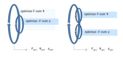
Figure 1: Schematic view of two iterative algorithms. On the left-hand side, the nested optimization method studied in this paper optimizes the pseudo free-energy over one field for each optimization step taken for the other field. On the right hand side, the other iterative method puts both optimization loops on the same level in a third encompassing loop.

Squared gradient

An alternative to the nested optimizations discused above is the use of a new functional based on the gradient of the free energy Borukhov, Andelman, and Orland (1999). At the saddle point

$$\left(\frac{\delta F}{\delta\phi}\right)_{\phi_{SP},\Psi_{SP}}=\left(\frac{\delta F}{\delta\Psi}\right)_{\phi_{SP},\Psi_{SP}}=0$$ (49)

We can build a new functional which is always positive and vanishes at the stationary point:

$$F_{deriv}(\phi,\Psi)=\int\left[\left(\frac{\delta F}{\delta\Psi}\right)^{2}+\left(\frac{\delta F}{\delta\phi}\right)^{2}\right]{\,\rm d}{\bf r}$$ (50)

The minimum of this functional yields the fields at equilibrium. The advantage of this formulation is that all fields can be treated equally by the minimization process which can be managed as a single global optimization.

Generalized scalar functionals

The next algorithm that we test is that based on eq. (37). We denote $\xi(\phi,\Psi)=\frac{\epsilon\nabla^{2}\phi+\sigma-pe\Psi^{2}}{e\lambda}$, and work with the free energy

$$F_{I}(\phi, \Psi)\>=\int\Big{[}\>k_{B}T\left\{\frac{a^{2}}{6}(\nabla\Psi)^{2}+\frac{v}{2}\Psi^{4}\right\}+\frac{\epsilon}{2}(\nabla\phi)^{2}$$

$$+ 2\lambda k_{B}T\>\Big{\{}-\cosh\left(\beta e\phi\right)\;+\;\beta e\phi\;\sinh(\beta e\phi)$$

$$- \;{{\rm sinh^{-1}}}(\xi/2)\;\sinh(\beta e\phi)+\;(\xi/2)\;{{\rm sinh^{-1}}}\left(\xi/2\right)\Big{\}}\Big{]}{\,\rm d}{\bf r}$$

The global minimum is found with a single optimization loop.

Legendre Transform

The Legendre transform of the electrostatic degrees of freedom is still possible in the presence of the extra polymer field. We find the locally defined free energy:

$$F_{L}({\bf D},\Psi)=\int \Big{[}k_{B}T\left\{\frac{a^{2}}{6}(\nabla\Psi)^{2}+\frac{v}{2}\Psi^{4}\right\}$$

$$+ \frac{{\bf D}^{2}}{2\epsilon}+k_{B}T\lambda g(\xi)\Big{]}{\,\rm d}{\bf r}$$

with $\xi={(\sigma-pe\Psi^{2}-{{\rm div}\;}{\bf D})}/{e\lambda}$. The minimum over both $\Psi$ and ${\bf D}$ is found with a single optimization loop.

Numerical Results

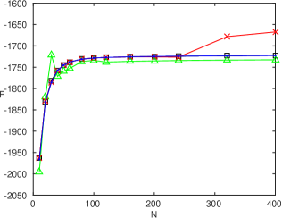
Figure 2: Convergence of free energy as a function of the number of points in the discretization. Blue dots ($\bullet$): Legendre transform. Green triangles: ($\vartriangle$) squared gradient. Black squares: ($\square$) nested loops. Red crosses ($\times$): generalized scalar functionals. Simple minimizer without external derivative information. Only the Legendre method reliably converges for all $N$.

The four functionals were programmed in Matlab. We use the function fminunc to search for the minimum for each case. This function uses a quasi-Newton algorithmDennis and More (1977) and in particular the Broyden-Fletche-Goldfarb-Shanno update. The idea is to use a good, black-box minimizer to study how each formulation converges in time and accuracy as the number of discretization points increase. The ideal is a formulation that converges to high accuracy without the need for detailed tuning of the algorithm for each application. We choose to stop iteration when the functional is converged to within an estimated fraction of $10^{-12}$.

Three quantities are considered to study the performance of each method:

• Convergence of $F$ when the number of points increase.

• The derivative of the functional with respect to each field. We use the $L_{1}$-norm to test the validity of the simulation

• Simulation time as a function of $N$.

Variables are initialized to $\Psi=1$ for the polyelectrolyte field and $\phi=-1$ for the potential. The system size is $24$ nm, where the charge of the capsid is $\sigma=0.4e$ at $R=12$ nm. The bulk concentration of monovalent ions is $\lambda=10\mbox{ mmol.L}^{-1}$ and the water relative permittivity is $\epsilon_{R}=80$. This corresponds to a Debye length of $3\text{ nm}$. The parameters of the polyelectrolyte are set to $a=0.5\text{ nm}$, $v=0.05\text{ nm}^{3}$, and $p=1$. The evolution of the free energies as a function of $N$ is depicted in Fig. (2); Fig. (3) shows the derivatives on stopping.

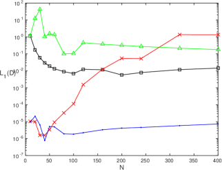
Figure 3: Color code as Fig. 2. Derivatives of the free energy for the virus model for different discretizations and methods on exit from the optimization loop.

We work with values of $N$ up to 400 which gives values of ($1/\kappa h$), eq. (44), up to 50. The discretizations are thus rather stiff. The most robust method appears to be that based on the Legendre transform. Indeed, it is the method that converges and gives the smallest error when the number of points is large, Fig. (2), Fig. (3). We note that the squared gradient method gives poor results with even small $N$ and the generalized scalar functional shows poor convergence for large $N$.

The simulation time of each method is shown in Fig. (4) as a function of discretization; we use a recent intel-based desktop computer. As expected the minimization time scales quadratically with the number of variables in the discretization. We tried other, random, initialisations and found that in all cases the method based on the Legendre transform gives the most stable results, together with a time of calculation which is as good as the other tested algorithms.

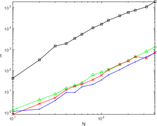
Figure 4: Color code as Fig. 2. Total simulation time as a function of the number of points in the discretization of the free energy. All algorithms display a quadratic growth in time with $N$. The algorithm based on the double loop is much slower than the three other methods. Dash line slope 2.

Stiffness and algorithms

From our numerical experiments we see that naive optimization of an expression with a saddle point leads to slow convergence. It is more surprising that some algorithms that can use convex optimization also give poor numerical results. One possible explanation for the differences observed between the three convex methods is that the algorithms have very different stiffnesses when the number of discretization points increases. As noted above an algorithm based on the Legendre transform has a stiffness which increases as $N^{2}$, whereas both the squared gradient and generalized scalar functionals become much stiffer with scaling in $N^{4}$. This renders numerical codes much more susceptible to numerical round-off errors and also requires more careful stopping criteria. However as stated above our philosophy is that we are looking for free energies that are stable and easy to use without large amounts of algorithmic tuning from the user.

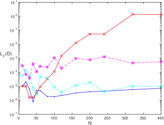
Figure 5: Derivatives of the free energy for the virus model for different discretizations and algorithms on exit from the optimization loop. Blue dots ($\bullet$): Legendre transform, quasi-Newton. Cyan circles ($\circ$): Legendre transform, trust-region. Red cross $\times$: scalar functional, quasi-Newton. Magenta stars ($\star$): scalar functional, trust-region.

More sophisticated black-box algorithms are also available. In particular if we are willing to calculate and program a routine which calculates the first derivative of the free energy with respect to each variable we can find better results. In particular we use another algorithm implemented in Matlab the trust-region algorithm Sorensen (1982). It avoids over-large steps thanks to the limit imposed by the definition of a trust-region, yet it maintains strong convergence properties. The L1-norm of the derivatives Fig. (5) and time used Fig. (6) are compared with the results obtained with the quasi-Newton algorithm. The change of algorithm allows one either to significantly reduce the computational time (Legendre transform method, blue and cyan points), or to better converge (generalized scalar functionals, red and magenta points. With the trust-region algorithm the lack of convergence of the free energy disappears). Thus, using the more sophisticated algorithm with derivative information renders the optimization more reliable or more efficient.

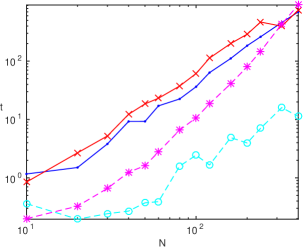
Figure 6: Color code as for Fig. 5. Computational time for different methods.

Conclusion

We have studied the quadratic fluctuations around equilibrium for several expressions for the free energy of charged media. These fluctuations are closely related to dispersion energies and the Debye-Hückel contribution to the free energy of electrolytes. The functional based on the field ${\bf D}$ correctly reproduces this free energy, even though the functional was originally proposed as a minimum principle.

When used in molecular dynamics codes it is important to chose functionals which are not too stiff. We emphasised that the ratio of the largest to smallest eigenvalue in the quadratic form is closely related to the number of time steps which are required to sample all modes. Again the functional based on the vector field ${\bf D}$ seems to display good scaling.

We used a model of a virus to implement and compare the optimization of four free energy functionals. The Legendre-transformed functional shows faster convergence and a greater accuracy in our tests. We suspect that this is linked to the lower stiffness of the Legendre formulation of the free energy.

Acknowledgment

Work financed in part by the ANR grant FSCF. We wish to thank Derek Frydel for discussions and critical readings of the manuscript.

Appendix: Spherical symmetry and discretisation

Our study of determinant identities brought out the importance of discretizations that conserve the adjoint relation between the divergence and gradient operators. Such identities are also important for our study of the minimization of the polyelectrolyte free energy. Non-compatible discretizations give rise to numerical errors which are different between the different formulations. We now show how to discretize within a spherical geometry in such a way as to include important dualities between the discretized equations. The potentials $\phi$ and $\Psi$ are defined on the points of the discretisation, while $\nabla\phi$, $\nabla\Psi$ and ${\bf D}$ are defined on intermediate links. We wish to conserve the fundamental identity

$$\int{\bf D}\cdot\nabla\phi=-\int\phi{{\rm div}\;}{\bf D}+\oint\phi{\bf D}\cdot dS$$ (51)

The discretized left hand side of this equation gives:

$$4\pi\sum_{n}r_{n,n+1}^{2}\left(\frac{\phi_{n+1}-\phi_{n}}{\delta}\right){\bf D}_{n,n+1}$$ (52)

where we have used the simplest differencing scheme for the gradient operator and we define $r_{n,n+1}$ as the position of the centre of the link. Identifying both sides of the identity, a definition of the discretized divergence is obtained:

$${{\rm div}\;}_{n}\;{\bf D}=\frac{{\bf D}_{n,n+1}\>r_{n,n+1}^{2}-{\bf D}_{n-1,n}\>r_{n-1,n}^{2}}{\delta\;r_{n}^{2}}$$ (53)

The Laplacian operator is then defined as usual by $\nabla^{2}=-{{\rm div}\;}_{n}\,{{\rm grad}\;}$.

Appendix: one-loop free energies

We give here the treatment of the one-loop correction in a homogeneous electrolyte. The free energy (compared with the free energy of an empty box) coming from quadratic fluctuations is

$$F_{f}= \frac{k_{B}T}{2}\sum_{q}\log(1+\frac{\kappa^{2}}{q^{2}})$$ (54)

$$= \frac{k_{B}T}{(2\pi)^{2}}\int_{0}^{q_{0}}q^{2}\,{\rm d}q\,\log(1+\kappa^{2}/q^{2})$$ (55)

$$= \frac{k_{B}T}{(2\pi)^{2}}\left(\kappa^{2}q_{0}-\frac{\pi\kappa^{3}}{3}\right)+O(1/q_{0})$$ (56)

Where we introduce an upper cut-off $q_{0}$. The divergence in $q_{0}^{1}$ can be balanced by a purely local self energy of the form $1/(2q^{2})$ corresponding to the Born energy $1/8\pi\epsilon a$ per atom, with $a$ a real-space cut-off. The long-ranged Debye-Hückel energy to the electrolyte is then

$$\frac{F_{DH}}{V}=-\frac{k_{B}T\kappa^{3}}{12\pi}$$ (57)

which comes from

$$F_{DH}=\frac{k_{B}T}{2}\sum_{q}\left(\log(1+\kappa^{2}/q^{2})-\lambda\beta e^{2}/(\epsilon q^{2})\right)$$ (58)

References

- Allen, Hansen, and Melchionna (2001) R. Allen, J.-P. Hansen, and S. Melchionna, “Electrostatic potential inside ionic solutions confined by dielectrics: a variational approach,” Phys. Chem. Chem. Phys. 3, 4177–4186 (2001).
- Fogolari and Briggs (1997) F. Fogolari and J. M. Briggs, “On the variational approach to Poisson-Boltzmann free energies,” Chemical Physics Letters 281, 135 – 139 (1997).
- Reiner and Radke (1990) E. S. Reiner and C. J. Radke, “Variational approach to the electrostatic free energy in charged colloidal suspensions: general theory for open systems,” Journal of the Chemical Society, Faraday Transactions 86, 3901–3912 (1990).
- Note (1) An exception is vanderbilt.
- Landau et al. (1984) L. Landau, E. Lifshits, E. Lifshits, and L. Pitaevskiĭ, Electrodynamics of continuous media:, Pergamon international library of science, technology, engineering, and social studies (Pergamon, 1984).
- Kirzhnits (1987) D. A. Kirzhnits, “General properties of electromagnetic response functions,” Soviet Physics Uspekhi 30, 575 (1987).
- Dolgov, Kirzhnits, and Maksimov (1981) O. Dolgov, D. Kirzhnits, and E. Maksimov, “On an admissible sign of the static dielectric function of matter,” Rev. Mod. Phys. 53, 81–93 (1981).
- Maggs (2012) A. C. Maggs, “A minimizing principle for the poisson-boltzmann equation,” EPL (Europhysics Letters) 98, 16012 (2012).
- Pujos and Maggs (2012) J. S. Pujos and A. C. Maggs, “Legendre transforms for electrostatic energies,” (2012), cite arxiv:1211.6601 Comment: 7 pages; CECAM workshop: New Challenges in Electrostatics of Soft and Disordered Matter (May 7, 2012 to May 10, 2012): http://www.cecam.org/workshop-0-689.html.
- Arnold et al. (2013) A. Arnold, K. Breitsprecher, F. Fahrenberger, S. Kesselheim, O. Lenz, and C. Holm, “Efficient algorithms for electrostatic interactions including dielectric contrasts,” Entropy 15, 4569–4588 (2013).
- Car and Parrinello (1985) R. Car and M. Parrinello, “Unified approach for molecular dynamics and density-functional theory,” Phys. Rev. Lett. 55, 2471–2474 (1985).
- Rottler and Maggs (2004) J. Rottler and A. C. Maggs, “Local molecular dynamics with Coulombic interactions,” Phys. Rev. Lett. 93, 170201 (2004).
- Jadhao, Solis, and de la Cruz (2013) V. Jadhao, F. J. Solis, and M. O. de la Cruz, “Free-energy functionals of the electrostatic potential for Poisson-Boltzmann theory,” Phys. Rev. E 88, 022305 (2013).
- Solis, Jadhao, and Olvera de la Cruz (2013) F. Solis, V. Jadhao, and M. Olvera de la Cruz, “Generating true minima in constrained variational formulations via modified Lagrange multipliers,” Phys. Rev. E 88, 053306 (2013).
- Jadhao, Solis, and de la Cruz (2012) V. Jadhao, F. Solis, and M. de la Cruz, “Simulation of charged systems in heterogeneous dielectric media via a true energy functional,” Phys. Rev. Lett. 109, 223905 (2012).
- Maggs (2004) A. C. Maggs, “Auxiliary field Monte Carlo for charged particles,” The Journal of Chemical Physics 120, 3108–3118 (2004).
- Maggs (2002) A. C. Maggs, “Dynamics of a local algorithm for simulating Coulomb interactions,” The Journal of Chemical Physics 117, 1975–1981 (2002).
- Pasquali and Maggs (2008) S. Pasquali and A. C. Maggs, “Fluctuation-induced interactions between dielectrics in general geometries,” The Journal of Chemical Physics 129, 014703 (2008).
- Podgornik and Zeks (1988) R. Podgornik and B. Zeks, “Inhomogeneous coulomb fluid. a functional integral approach,” J. Chem. Soc., Faraday Trans. 2 84, 611–631 (1988).
- Netz and Orland (1999) R. R. Netz and H. Orland, “Field theory for charged fluids and colloids,” EPL (Europhysics Letters) 45, 726 (1999).
- Wang (2010) Z.-G. Wang, “Fluctuation in electrolyte solutions: The self energy,” Phys. Rev. E 81, 021501 (2010).
- Zia, Redish, and McKay (2009) R. K. P. Zia, E. F. Redish, and S. R. McKay, “Making sense of the Legendre transform,” American Journal of Physics 77, 614–622 (2009).
- Buyukdagli, Achim, and Ala-Nissila (2012) S. Buyukdagli, C. V. Achim, and T. Ala-Nissila, “Electrostatic correlations in inhomogeneous charged fluids beyond loop expansion,” J. Chem. Phys. 137, 104902 (2012).
- Buyukdagli and Ala-Nissila (2014) S. Buyukdagli and T. Ala-Nissila, “Electrostatic correlations on the ionic selectivity of cylindrical membrane nanopores,” The Journal of Chemical Physics 140, 064701 (2014).
- Naji et al. (2013) A. Naji, M. Kanduč, J. Forsman, and R. Podgornik, “Perspective: Coulomb fluids—weak coupling, strong coupling, in between and beyond,” The Journal of Chemical Physics 139, 150901 (2013).
- Xu and Maggs (2014) Z. Xu and A. Maggs, “Solving fluctuation-enhanced Poisson-Boltzmann equations,” Journal of Computational Physics 275, 310 – 322 (2014).
- Koehl and Delarue (2010) P. Koehl and M. Delarue, “Aquasol: An efficient solver for the dipolar Poisson–Boltzmann–Langevin equation,” The Journal of Chemical Physics 132, 064101 (2010).
- Lu et al. (2008) B. Lu, Y. Zhou, M. Holst, and J. McCammon, “Recent progress in numerical methods for the Poisson–Boltzmann equation in biophysical applications,” Communications in Computational Physics 3, 973–1009 (2008).
- Edwards (1965) S. F. Edwards, “The statistical mechanics of polymers with excluded volume,” Proceedings of the Physical Society 85, 613 (1965).
- de Gennes (1979) P.-G. de Gennes, “Scaling concepts in polymer physics,” (Cornell University Press, 1979) Chap. IX.2. Self-Consistent Fields.
- Šiber and Podgornik (2008) A. Šiber and R. Podgornik, “Nonspecific interactions in spontaneous assembly of empty versus functional single-stranded rna viruses,” Phys. Rev. E 78, 051915 (2008).
- Siber, Bozic, and Podgornik (2012) A. Siber, A. L. Bozic, and R. Podgornik, “Energies and pressures in viruses: contribution of nonspecific electrostatic interactions,” Phys. Chem. Chem. Phys. 14, 3746–3765 (2012).
- Borukhov, Andelman, and Orland (1999) I. Borukhov, D. Andelman, and H. Orland, “Effect of polyelectrolyte adsorption on intercolloidal forces,” The Journal of Physical Chemistry B 103, 5042–5057 (1999), http://pubs.acs.org/doi/pdf/10.1021/jp990055r .
- Dennis and More (1977) J. Dennis, J. E. and J. J. More, “Quasi-Newton methods, motivation and theory,” SIAM Review 19, pp. 46–89 (1977).
- Note (2) As is required too in molecular dynamics; these derivatives are already calculated for the square gradient method.
- Sorensen (1982) D. C. Sorensen, “Newton’s method with a model trust region modification,” SIAM Journal on Numerical Analysis 19, pp. 409–426 (1982).