Dicke simulators with emergent collective quantum computational abilities

Abstract

Using an approach inspired from Spin Glasses, we show that the multimode disordered Dicke model is equivalent to a quantum Hopfield network. We propose variational ground states for the system at zero temperature, which we conjecture to be exact in the thermodynamic limit. These ground states contain the information on the disordered qubit-photon couplings. These results lead to two intriguing physical implications. First, once the qubit-photon couplings can be engineered, it should be possible to build scalable pattern-storing systems whose dynamics is governed by quantum laws. Second, we argue with an example how such Dicke quantum simulators might be used as a solver of “hard” combinatorial optimization problems.

The connection of experimentally realizable quantum systems with computation contains promising perspectives from both the fundamental and the technological viewpoint Feynman (1982); Nielsen and Chuang (2010). For example, quantum computational capabilities can be implemented by “quantum gates” Barenco et al. (1995) and by the so-called “adiabatic quantum optimization” technique Farhi et al. (2001); Santoro et al. (2002); Bapst et al. . Today’s experimental technology of highly controllable quantum simulators, recently used for testing theoretical predictions in a wide range of areas of physics Buluta and Nori (2009); Georgescu et al. (2014); Lewenstein et al. (2007), offers new opportunities for exploring computing power for quantum systems.

In the case of light-matter interaction at the quantum level, the reference benchmark is the Dicke model Dicke (1954). Studies of its equilibrium properties have predicted a superradiant transition to occur in the strong coupling and low temperature regime Hepp and Lieb (1973a, b); Wang and Hioe (1973). The superradiant phase is characterized by a macroscopic number of atoms in the excited state whose collective behaviour produces an enhancement of spontaneous emission (proportional to the number of cooperating atoms in the sample). Crucially, this phenomenology is in direct link with experimentally feasible quantum simulators. Recently, Nagy and coworkers Nagy et al. (2010) argued that the Dicke model effectively describes the self-organization phase transition of a Bose-Einstein condensate (BEC) in an optical cavity Baumann et al. (2010, 2011). Additionally, Dimer and colleagues Dimer et al. (2007) proposed a Cavity QED realization of the Dicke model based on cavity-mediated Raman transitions, closer in spirit to the original Dicke’s idea. Evidence of superradiance in this system is reported in Baden et al. (2014). An implementation of generalized Dicke models in hybrid quantum systems has also been put forward Zou et al. (2014). More generally, Dicke-like Hamiltonians describe a variety of physical systems, ranging from Circuit QED Zhang et al. (2014); Nataf and Ciuti (2010); Viehmann et al. (2011); Mlynek et al. (2014); Mezzacapo et al. (2014) to Cavity QED with Dirac fermions in graphene Chirolli et al. (2012); Hagenmüller and Ciuti (2012); Pellegrino et al. (2014). Additionally, disorder and frustration of the atom-photon couplings have an important role in the study of BEC in multimode cavities Gopalakrishnan et al. (2009, 2010). Recent works Gopalakrishnan et al. (2011); Strack and Sachdev (2011) discussed a multimodal-Cavity QED simulator with disordered interactions. The authors argue that these systems could be employed to explore spin-glass properties at the quantum level Gopalakrishnan et al. (2011); Strack and Sachdev (2011); Rotondo et al. (2015). However, the possible quantum computation applications of this new class of quantum simulators remain relatively unexplored.

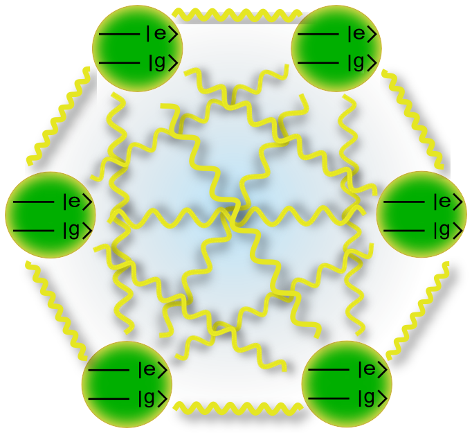
Figure 1: In the Dicke model, photons (yellow lines) mediate a long range interaction between qubits (green circles). The drawing sketches schematically a six qubits system within its fully-connected graph and its internal level structure. In the standard single-mode Dicke model the exchange coupling is fixed at the same value for every pair of qubits. In systems where both many modes and disorder are present, the exchange couplings are qubit-dependent and take the form given by Eq. (3).

In this Letter, we consider a multimode disordered Dicke model with finite number of modes. We calculate exactly (in the thermodynamic limit) the free energy of the system at temperature $T=1/\beta$ and we find a superradiant phase transition characterized by the same free-energy landscape of the Hopfield model Hopfield (1982) in the so-called “symmetry broken” phase, with the typical strong-coupling threshold of the Dicke model. From the theoretical standpoint, our results generalize to the case of quenched disordered couplings the remarkable analysis performed by Lieb et al. Hepp and Lieb (1973a, b); Wang and Hioe (1973). The choice of frozen couplings is compatible with the characteristic time scales involved in light-matter interactions. The calculation of the partition function leads us to suggest variational ground states for the model, which we conjecture to be exact in the thermodynamic limit.

The physical consequences of this analysis are fascinating: once the multimode strong-coupling regime is reached and qubit-photon couplings are engineered, it should be possible to build a pattern-storing system whose underlying dynamics is fully governed by quantum laws. Moreover, Dicke quantum simulators here analyzed may be suitable to implement specific optimization problems, in the spirit of adiabatic quantum computation Bapst et al. ; Farhi et al. (2001); Santoro et al. (2002). We point out a non-polynomial optimization problem Lucas (2014); Farhi et al. (2001); Santoro et al. (2002), number partitioning, which could be implemented in a single mode cavity QED setup with controllable disorder. Computing applications based on cavity mediated interactions might owns the advantage to be a viable way to generate entagled many-body states with remarkable scalability properties, as recently shown in Ref. Aron et al. (2014).

Hopfield’s main idea Hopfield (1982) is that the retrieval of stored information, such as memory patterns, may emerge as a collective dynamical property of microscopic constituents (“neurons”) whose interconnections (“synapses”) are reinforced or weakened through a training phase (e.g. Hebbian learning Hebb (1940, 1961)). This is achieved in his model through a fictitious neuronal-dynamics whose effect is to minimize the Lyapunov cost function:

$$E=-\frac{1}{2}\sum_{i,j=1}^{N}T_{ij}S_{i}S_{j}\,,$$ (1)

where $N$ is the number of neurons, $S_{i}=1$ if the $i$-th neuron is active, and $-1$ otherwise, and the $p$ stored patterns $\xi_{i}^{(k)}=\pm 1$ ($k=1,\cdots,p$) determine the interconnections $T_{ij}$ through the relation: $T_{ij}=1/N\sum_{k}\xi_{i}^{(k)}\xi_{j}^{(k)}-p\,\delta_{ij}$. The analysis in Ref. Hopfield (1982) shows that the long-time dynamics always converges to one of the $p$ stored patterns, i.e. these configurations are the global minima of the cost function (1). The interpretation of this result is that a suitable choice of the interconnections allows to store a given number of memory patterns into the neural network. Data retrieval is achieved through an algorithm that minimizes the energy function (1). A phase transition to a “complex” phase marks the intrinsic limitation on the number of patterns $p$ that can be stored. If $p$ exceeds the critical threshold $p\sim 0.14N$ many failures in the process of retrieval occur Amit et al. (1985a, b).

In this manuscript we consider the following multimode Dicke Hamiltonian:

$$H=\sum_{k=1}^{M}\omega a^{\dagger}_{k}a^{\phantom{{}^{\prime}}}_{k}+\Delta\sum_{i=1}^{N}\sigma^{z}_{i}+\sum_{i,k=1}^{N,M}\tilde{g}_{ik}\left(a^{\phantom{{}^{\prime}}}_{k}+a_{k}^{\dagger}\right)\sigma^{x}_{i}\,,$$ (2)

effectively modelling quantum light-matter interaction of $N$ two-level systems with detuning $\Delta$ and $M$ electromagnetic modes supposed to be quasi-degenerate at the common frequency $\omega$ and with couplings that we parametrize for future convenience as $\tilde{g}_{ik}=\Omega g_{ik}/\sqrt{N}$, where $\Omega$ is the Rabi frequency and the dimensionless $g_{ik}$’s are both atom and mode-dependent. In Cavity QED realizations, $\omega$ represents the detuning between the cavity frequency and the pumping frequency and could be both positive or negative. A possible choice of the couplings is $g_{il}=\cos(k_{l}x_{i})$, being $k_{l}$ the wave vector of the photon and $x_{i}$ the position of $i$-th atom Strack and Sachdev (2011).

We are interested in the thermodynamic properties of this system in the limit $M\ll N$, and thus in evaluating the partition function $Z=\operatorname{Tr}e^{-\beta H}$. This evaluation can be performed rigorously in the thermodynamic limit ($N\rightarrow\infty$) using the techniques introduced in Refs. Hepp and Lieb (1973a, b); Wang and Hioe (1973). We first consider the fully-commuting limit $\Delta=0$. In this case the evaluation of the partition function is straightforward (see Supplementary material) and we obtain $Z=Z_{FB}\,Z_{H}$, where $Z_{FB}$ is a free boson partition function and $Z_{H}$ is a classical Ising model with local quenched exchange interactions of the form:

$$J_{ij}=-\frac{\Omega^{2}}{N}\sum_{k=1}^{M}\frac{g_{ik}\,g_{jk}}{\omega}\,.$$ (3)

The physical interpretation of this result is that photons mediate long range interactions among the atoms, resulting in an atomic effective Hamiltonian described by a fully-connected Ising model (see Fig. 1). The role of the couplings $g_{ik}$ can be understood from Eq. (1) in the context of the Hopfield network. They are the memory pattern stored in the system. By computing exactly the free energy of the model, we will show that this interpretation stays unaltered in the more complicated case $\Delta\neq 0$.

We now proceed to the evaluation of the quantum partition function. We use the method of Wang and coworkers Wang and Hioe (1973); Larson and Lewenstein (2009) (proved to be exact in the thermodynamic limit for $M/N\rightarrow 0$ Hepp and Lieb (1973b)). We introduce a set of coherent states $\ket{\alpha_{k}}$ with $\alpha_{k}=x_{k}+iy_{k}$, one for each electromagnetic mode $k$, and we expand the partition function on this overcomplete basis:

$$Z=\int\prod_{k=1}^{M}\frac{d^{2}\alpha_{k}}{\pi}\,\operatorname{Tr}_{A}\bra{\{\alpha\}}e^{-\beta H}\ket{\{\alpha\}}\,,$$ (4)

where $\operatorname{Tr}_{A}$ is the atomic trace only. The only technical complication is the calculation of the matrix element in (4). This turns out to be equal, apart from non-extensive contributions, to the exponential of the operator in Eq (2) with the replacements $a_{k},~{}a^{\dagger}_{k}\rightarrow\alpha_{k},~{}\alpha_{k}^{\ast}$  Wang and Hioe (1973); Hepp and Lieb (1973b). At this stage the trace over the atomic degrees of freedom can be easily performed. The integral over the imaginary parts of $\alpha_{k}$’s give an overall unimportant constant. Finally, defining the $M$-dimensional vectors $\mathbf{x}=(x_{1},x_{2},\cdots,x_{M})$ and $\mathbf{g}_{i}=(g_{i1},g_{i2},\cdots,g_{iM})$, and with the change of variables $\mathbf{m}=\mathbf{x}/\sqrt{N}$, the partition function assumes a suitable form for performing a saddle-point integration, i.e. $Z=\int\,d^{M}\mathbf{m}\,e^{-Nf(\mathbf{m})}$. Here $f$ is the free energy

$$f(\mathbf{m})=\beta\mathbf{m}\cdot\mathbf{m}-\frac{1}{N}\sum_{i=1}^{N}\log G(\mathbf{m},\mathbf{g}_{i})\,,$$ (5)

with: $G(\mathbf{m},\mathbf{g}_{i})=2\cosh\left[\beta\left(\Delta^{2}+\Omega^{2}(\mathbf{g}_{i}\cdot\mathbf{m})^{2}\right)^{\frac{1}{2}}\right]$.

The order parameter $\mathbf{m}$ describes the superradiant phase transition. Physically, it gives the mean number of photons in every mode Emary and Brandes (2003). Its value is determined by minimizing the free energy in Eq.  (5). Solutions of this optimization problem are, in principle, $\mathbf{g}_{i}$-dependent, but in the thermodynamic limit both the free energy and the saddle-point equation are self-averaging Amit et al. (1985a). Thus we conclude that the free energy and the saddle point equations are given by

$$f(\mathbf{m}) =\beta\mathbf{m}\cdot\mathbf{m}-\Braket{\log G(\mathbf{m},\mathbf{g})}_{\mathbf{g}}\,,$$

$$\mathbf{m} =\frac{\Omega^{2}}{2}\Braket{\frac{(\mathbf{g}\cdot\mathbf{m})\,\mathbf{g}}{\mu(\mathbf{g})}\tanh\left(\beta\mu(\mathbf{g})\right)}_{\mathbf{g}}\,,$$ (6)

with: $\mu(\mathbf{g})=\left(\Delta^{2}+\Omega^{2}(\mathbf{g}\cdot\mathbf{m})^{2}\right)^{\frac{1}{2}}$ and $\braket{\cdots}_{\mathbf{g}}$ representing the average over the disorder distribution. Eq. (6) reduces to the mean-field equations for the Hopfield model for $\Delta\rightarrow 0$ Amit et al. (1985a). Thus, $\Delta$ may be intended as a quantum annealer parameter. To fully specify the model, the probability distribution for the couplings is needed. In the following we will assume

$$P(\mathbf{g})=\prod_{k=1}^{M}\left(\frac{1}{2}\delta\left(g_{k}-1\right)+\frac{1}{2}\delta\left(g_{k}+1\right)\right)\,,$$ (7)

but we have verified that the results are qualitatively robust as long as the disorder is not too peaked around zero in accordance with the classical results of Ref. Amit et al. (1985a) To locate the critical point it suffices to expand in Taylor series Eqs. (6). As in the conventional Dicke model, a temperature-independent threshold $\Omega_{c}^{2}=2\Delta$ emerges. For $\Omega<\Omega_{c}$, the phase transition is inhibited at all temperatures. Whenever the magnitude of the coupling exceeds this threshold value, the critical temperature is located at $T_{c}=\Delta/\operatorname{arctanh}\left(2\Delta/\Omega^{2}\right)$.

Above the critical temperature $T_{c}$ the only solution to (6) is a paramagnetic state, with $m_{k}=0$ for all $k$. Below $T_{c}$, different solutions appear. We now set out to classify these solutions and their stability under temperature decrease. For this analysis, we both considered the Hessian matrix $\partial^{2}{f}/\partial{m_{k}}\partial{m_{l}}$ (see Supplementary materials for its explicit expression) and numerical optimization (Figure 2) . The key point, as mentioned above is that in this “symmetry-broken” phase the system takes $2M$ degenerate ground states (as well as many metastable states energetically well separated from the ground states). In other words, also in this fully quantum limit the free-energy landscape still closely resembles that of the Hopfield model Amit et al. (1985a).

The ground state solutions have the explicit form:

$$\mathbf{m}_{k}=m^{(1)}(\underbrace{0,0,\cdots,0}_{k-1\,\,times},\underbrace{1,0,\cdots,0}_{M-k+1\,\,times})\,.$$ (8)

Equation (6) for the order parameter $m^{(1)}$ reduces to: $2\mu(m^{(1)})=\Omega^{2}\tanh\left(\beta\mu(m^{(1)})\right)$, where $\mu(m^{(1)})=\sqrt{\Delta^{2}+\Omega^{2}(m^{(1)})^{2}}$. In the zero temperature limit the order parameter can be evaluated exactly:

$$m^{(1)}=\pm\sqrt{\frac{\Omega^{2}}{4}-\frac{\Delta^{2}}{\Omega^{2}}}\,.$$ (9)

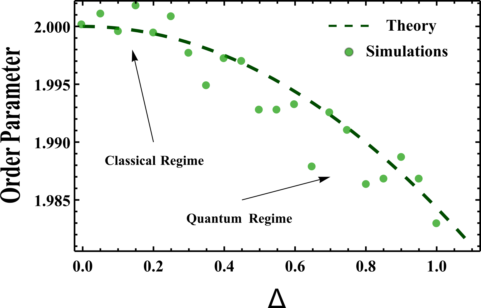
Figure 2: Order parameter $m^{(1)}$ in Eq. (9) as a function of $\Delta$ in the ultrastrong coupling regime at $T=0$. On the theoretical curve (dashed line) are superposed the results (green dots) of a naive numerical optimization algorithm minimizing the ground state energy ansatz in Eq. (11). The parameters of the simulation are $\Omega=4$, $N=100$, $M=10$. Green dots are the result of a single disorder realization. This implies the correctness of our self-averaging hypothesis, which is a good approximation already for $N=100$. The classical Hopfield model is recovered in the limit $\Delta\rightarrow 0$.

At zero temperature the most interesting state is the ground state (GS) of the Hamiltonian (2). Inspired by the calculation above we propose the variational ansatz for the GS:

$$\ket{GS}=\ket{\alpha_{1},\alpha_{2},\cdots,\alpha_{M}}\ket{\text{spin}(\alpha_{1},\cdots,\alpha_{M})}\,,$$ (10)

where $\ket{\alpha_{1},\alpha_{2},\cdots,\alpha_{M}}$ is the product of $M$ coherent states and the spin part is factorized. The mean value of the energy in this GS is given by:

$$E_{GS}(\mathbf{m})=\mathbf{m}\cdot\mathbf{m}-\Braket{\sqrt{\Delta^{2}+\Omega^{2}(\mathbf{g}\cdot\mathbf{m})^{2}}}_{\mathbf{g}}\,.$$ (11)

This expression exactly equals the free-energy computed previously in the limit $\beta\rightarrow\infty$, which leads us to conjecture that our factorized variational ansatz is exact. The quantum phase transition is located at the critical coupling $\Omega=\Omega_{c}=\sqrt{2\Delta}$, at which the paramagnetic solution becomes unstable. In the symmetry-broken phase we have $2M$ degenerate ground states of the form

$$\ket{GS}_{k}=\ket{\underbrace{0,0,\cdots,0}_{k-1\,times},\pm m^{(1)},\underbrace{0,\cdots,0}_{M-k\,times}}\ket{\text{spin}(\pm m^{(1)})}_{k}\,,$$ (12)

with $k=1,\cdots M$. The spin wave function is also factorized $\ket{\text{spin}(\pm m^{(1)})}_{k}=\prod_{i}\ket{s_{i}}_{k}$, with

$$\ket{s_{i}}_{k}=\frac{1}{\mathcal{N}}\left(-\frac{-\Delta+\sqrt{\Delta^{2}+\beta_{ik}^{2}}}{\beta_{ik}}\ket{e_{i}}+\ket{g_{i}}\right)\,,$$ (13)

where $\mathcal{N}$ a normalization, $\beta_{ik}=g_{ik}m^{(1)}$ and $\ket{e_{i}}$, $\ket{g_{i}}$ are $\sigma_{i}^{z}$’s eigenstates. It is worth noting that, as expected, the ground state energy is a self-averaging quantity, whereas the ground states are not, being disorder-dependent also in the thermodynamic limit.

The above calculation shows that in the superradiant phase the ground state of the system is a quantum superposition of the $2M$ degenerate eigenvectors given by Eqs. (12,13). Their explicit form suggests that at fixed disorder and mode number the information about the disordered couplings belonging to the $k$-th mode is printed on the atomic wave function. Moreover, the photonic parts of the wave functions are all orthogonal for $k_{1}\neq k_{2}$ in the thermodynamic limit. This implies that in principle a suitable measure on the photons-subsystem causes the collapse over one of the $2M$ ground states and gives thus the possibility to retrieve information (“patterns”) stored in the atomic wave function. As mentioned above, a single-mode Dicke model has been recently realized with cavity-mediated Raman transitions in cavity QED with ultracold atoms Baden et al. (2014). A Multimode cavity QED setup supporting disordered couplings has been proposed in refs. Gopalakrishnan et al. (2011); Strack and Sachdev (2011), and preliminary evidence of superradiance in this system is found in Wickenbrock et al. (2013). A setup operating in multimode regime has been recently suggested also in Circuit QED Egger and Wilhelm (2013). We are not aware of a setup (in Cavity or Circuit QED) that implements both multimode strong coupling regime and controllable disorder, a necessary condition for the quantum pattern-retrieval system that we conjecture here.

We surmise that Multimode Dicke quantum setups with controllable disorder could be used beyond storage, to simulate specific optimization problems. Indeed, finding the ground state of classical spin models with disordered interactions is equivalent, in most cases, to finding solutions of computationally expensive non-polynomial (NP) problems Lucas (2014). For example, the simplest NP-hard problem, number partitioning, could be implemented in a single-mode cavity QED setup with controllable disorder as follows. Number partitioning can be formulated as an optimization problem Mertens (1998): given a set $\mathcal{A}=\{a_{1},a_{2},\dots,a_{N}\}$ of positive numbers, find a partition, i.e. a subset $\mathcal{A}^{\prime}\subset\mathcal{A}$, such that the residue: $E=|\sum_{a_{j}\in\mathcal{A}^{\prime}}a_{j}-\sum_{a_{j}\notin\mathcal{A}^{\prime}}a_{j}\,|$ is minimized. A partition can be defined by numbers $S_{j}=\pm 1$: $S_{j}=1$ if $a_{j}\in\mathcal{A}^{\prime}$, $S_{j}=-1$ otherwise. The cost function can be replaced by a classical spin hamiltonian, whose ground state is equivalent to the minimum partition:

$$H=\sum_{i,j=1}^{N}a_{i}a_{j}S_{i}S_{j}\,.$$ (14)

In a single mode cavity QED network couplings can be chosen as $g_{i}=\cos(kx_{i})$ Strack and Sachdev (2011). By the definition of $a=~{}\max_{\mathcal{A}}a_{j}$ and $\tilde{a}_{j}=a_{j}/a$, it is possible to engineer the $g_{i}$’s in such a way to implement a given instance of the problem provided that the cavity is in the “blue” detuned regime to ensure the appropriate sign for the couplings, see Eq. (3). With a suitable adiabatic annealing of the atomic detuning $\Delta$, the system should collapse on qubit configurations that are good solutions of the corresponding optimization problem.

In conclusion, this Letter provides the first rigorous analysis of the multimode disordered Dicke model, valid beyond the weak-coupling regime and exact in the thermodynamic limit. The equivalence between multimodal disordered Dicke model and a quantum Hopfield network Nonomura and Nishimori (1995), together with the proposal of a cavity QED setup implementing a non polynomial optimization problem, demonstrates the possibility of quantum computational abilities of this new class of quantum simulators. Our proposal is conceptually complementary to a standard quantum computation perspective Loss and DiVincenzo (1998); Raussendorf et al. (2003). Indeed, the information can be “written” on the qubits through a quantum annealing on the detuning $\Delta$, similarly to what happens for adiabatic quantum computation Farhi et al. (2001); Santoro et al. (2002); Bapst et al. .

Acknowledgements.— We are grateful to B. Bassetti, S. Mandrà, G. Catelani, M. Gherardi, S. Caracciolo, L. Molinari, F. Solgun and A. Morales for useful discussions and feedback on this manuscript. GV was supported by Alexander von Humboldt foundation and Knut och Alice Wallenbergs foundation.

Dicke simulators with emergent collective quantum computational abilities
supporting material

Pietro Rotondo, Marco Cosentino Lagomarsino, and Giovanni Viola

In this material, we give more details on the derivations of the results presented in the main text.

S.I Derivation of Equation (3)

We begin with the derivation of Eq. (3), of the main text. We consider the partition function $Z=\mathrm{Tr}e^{-\beta H}$ with $H$ given in Eq. (2) for $\Delta=0$. In this fully commuting limit we can evaluate the partition function straightforwardly. We introduce new set of bosonic operators:

$$b^{\dagger}_{k}=a^{\dagger}_{k}+\frac{\Omega}{\omega\sqrt{N}}\sum_{i=1}^{N}g_{ik}\sigma^{x}_{i}\,,\qquad b_{k}=a_{k}+\frac{\Omega}{\omega\sqrt{N}}\sum_{i=1}^{N}g_{ik}\sigma^{x}_{i}\,.$$ (S.1)

with $[b_{k^{\prime}},b^{\dagger}_{k}]=\delta_{k,k^{\prime}}$. By means of those, $H$ is written as the sum of two commuting operators:

$$H=\omega\sum_{k=1}^{M}b^{\dagger}_{k}b^{\phantom{\dagger}}_{k}-\frac{\Omega^{2}}{N\omega}\sum_{i,j=1}^{N}\sum_{k=1}^{M}g_{ik}g_{jk}\sigma^{x}_{i}\sigma^{x}_{j}$$ (S.2)

As a byproduct we obtain the factorization of the full partition function S (1):$Z=Z_{B}\,Z_{H}$, where $Z_{B}$ is an overall free boson partition function that we can safely ignore in the thermodynamic limit. On the other hand

$$Z_{H}=\mathrm{Tr}_{\sigma}\exp\left(\beta\sum_{i,j}J_{ij}\sigma_{i}\sigma_{j}\right)$$ (S.3)

is an Ising contribution with both spin and mode dependent couplings $J_{ij}$ of the form given in Eq. (3) of the main text. In Eq.(S.3) $\mathrm{Tr}_{\sigma}$ indicates the trace on the spins only.

S.II Derivation of Equation (5)

In this section we report the derivation of Eq. (5) of the main text, which essentially follows the derivation of Wang and Hioe S (2) proved to be rigorous by Hepp and Lieb S (3). The authors of Ref. S (2) have shown explicitly, in the termodynamic limit, that the convenient way to calculate the trace on the Hilbert space of bosons, in the partition function, is to evaluate it on the set of the coherent states $|\{\alpha\}\rangle$. The photonic matrix element in the partition function of Eq. (4) equals in the thermodynamic limit ($\alpha_{k}=x_{k}+iy_{k}$):

$$\bra{\{\alpha\}}e^{-\beta H}\ket{\{\alpha\}}\simeq\exp\left(-\beta\omega\sum_{k=1}^{M}(x_{k}^{2}+y_{k}^{2})-\beta\Delta\sum_{i=1}^{N}\sigma^{z}_{i}-\beta\frac{\Omega}{\sqrt{N}}\sum_{i=1}^{N}\sum_{k=1}^{M}g_{ik}x_{k}\sigma^{x}_{i}\right)\,.$$ (S.4)

The atomic trace thus factorizes and it can be calculated:

$$Z=\int\prod_{k=1}^{M}\,\frac{dx_{k}\,dy_{k}}{\pi}\,e^{-\beta\omega\sum_{k=1}^{M}(x_{k}^{2}+y_{k}^{2})}\prod_{i=1}^{N}\cosh\left(\beta\sqrt{\Delta^{2}+\frac{\Omega^{2}}{N}\left(\sum_{k=1}^{M}g_{ik}x_{k}\right)^{2}}\right)=\int\prod_{k=1}^{M}\,\frac{dm_{k}}{\pi}e^{-Nf(\mathbf{m},\beta)}\,.$$ (S.5)

In the last term we introduced the vectorial notation defined in the main text. The final expression for the free energy is:

$$f(\mathbf{m},\beta)=\beta\mathbf{m}\cdot\mathbf{m}-\frac{1}{N}\sum_{i=1}^{N}\log\cosh\left(\beta\sqrt{\Delta^{2}+\frac{\Omega^{2}}{N}\left(\mathbf{g}_{i}\cdot\mathbf{m}\right)^{2}}\right)\,,$$ (S.6)

By minimizing the free energy above and using the self averaging property of Eq. (S.6), we obtain the exact mean field equations:

$$\mathbf{m}=\frac{\Omega^{2}}{2}\Braket{\frac{(\mathbf{g}\cdot\mathbf{m})\,\mathbf{g}}{\mu(\mathbf{g})}\tanh\left(\beta\mu(\mathbf{g})\right)}_{\mathbf{g}}$$ (S.7)

To locate the critical point it suffices to expand in Taylor series Eqs. (S.6),(S.7):

$$f(\mathbf{m})-f(\mathbf{0}) =\beta\left(1-\frac{\Omega^{2}}{2\Delta}\tanh(\beta\Delta)\right)\mathbf{m}\cdot\mathbf{m}+O\left(m_{k}^{4}\right)\,,\qquad m_{k}=\frac{\Omega^{2}}{2\Delta}\tanh(\beta\Delta)\,m_{k}+O(m_{k}^{3})\,.$$ (S.8)

As in the conventional Dicke model, a temperature-independent threshold $\Omega_{c}^{2}=2\Delta$ emerges. For $\Omega<\Omega_{c}$, the phase transition is inhibited at all temperatures. Whenever the magnitude of the coupling exceeds this threshold value, the critical temperature is located at $T_{c}=\Delta/\operatorname{arctanh}\left(2\Delta/\Omega^{2}\right)$. Solutions to Eq. (S.7) can be classified according to the number of non-zero components $n$ of the order parameter $\mathbf{m}$ S (4):

$$\mathbf{m}_{n}=m^{(n)}(\underbrace{1,1,\cdots,1}_{n\,\,times},\underbrace{0,0,\cdots,0}_{M-n\,\,times})\,,$$ (S.9)

where all permutations are also possible. In particular, solutions for $n=1$ are the ones with the lowest free energy. There are $2M$ of such solutions, corresponding to the $\mathbb{Z}_{2}\times S_{M}$ symmetry breaking of our multimode Dicke model.

For completeness we report the explicit expression for the Hessian matrix of the free energy, omitted in the main text for space imitations:

$$\frac{\partial^{2}{f}}{\partial{m_{k}}\partial{m_{l}}}=2\delta_{kl}-\Omega^{2}\Braket{\frac{g_{k}g_{l}}{\mu(\mathbf{g})}\tanh\left(\beta\mu(\mathbf{g})\right)}_{\mathbf{g}}+\Omega^{4}\Braket{\frac{(\mathbf{g}\cdot\mathbf{m})^{2}\,g_{k}g_{l}}{\mu(\mathbf{g})^{2}}\left[\frac{\tanh\left(\beta\mu(\mathbf{g})\right)}{\mu(\mathbf{g})}+\beta\mathrm{sech}^{2}\left(\beta\mu(\mathbf{g})\right)\right]}_{\mathbf{g}}\,.$$ (S.10)

References

- Feynman (1982) R. P. Feynman, International Journal of Theoretical Physics 21, 467 (1982).
- Nielsen and Chuang (2010) M. A. Nielsen and I. L. Chuang, Quantum computation and quantum information (Cambridge university press, 2010).
- Barenco et al. (1995) A. Barenco, C. H. Bennett, R. Cleve, D. P. DiVincenzo, N. Margolus, P. Shor, T. Sleator, J. A. Smolin, and H. Weinfurter, Phys. Rev. A 52, 3457 (1995).
- Farhi et al. (2001) E. Farhi, J. Goldstone, S. Gutmann, J. Lapan, A. Lundgren, and D. Preda, Science 292, 472 (2001).
- Santoro et al. (2002) G. E. Santoro, R. Martoňák, E. Tosatti, and R. Car, Science 295, 2427 (2002).
- (6) V. Bapst, L. Foini, F. Krzakala, G. Semerjian, and F. Zamponi, .
- Buluta and Nori (2009) I. Buluta and F. Nori, Science 326, 108 (2009).
- Georgescu et al. (2014) I. M. Georgescu, S. Ashhab, and F. Nori, Rev. Mod. Phys. 86, 153 (2014).
- Lewenstein et al. (2007) M. Lewenstein, A. Sanpera, V. Ahufinger, B. Damski, A. Sen, and U. Sen, Advances in Physics 56, 243 (2007).
- Dicke (1954) R. Dicke, Phys. Rev. 93, 99 (1954).
- Hepp and Lieb (1973a) K. Hepp and E. Lieb, Ann. Phys. 76, 360 (1973a).
- Hepp and Lieb (1973b) K. Hepp and E. Lieb, Phys. Rev. A 8, 2517 (1973b).
- Wang and Hioe (1973) Y. K. Wang and F. T. Hioe, Phys. Rev. A 7, 831 (1973).
- Nagy et al. (2010) D. Nagy, G. Kónya, G. Szirmai, and P. Domokos, Phys. Rev. Lett. 104, 130401 (2010).
- Baumann et al. (2010) K. Baumann, C. Guerlin, F. Brenneke, and T. Esslinger, Nature (London) 464, 1301 (2010).
- Baumann et al. (2011) K. Baumann, R. Mottl, F. Brennecke, and T. Esslinger, Phys. Rev. Lett. 107, 140402 (2011).
- Dimer et al. (2007) F. Dimer, B. Estienne, A. S. Parkins, and H. J. Carmichael, Phys. Rev. A 75, 013804 (2007).
- Baden et al. (2014) M. P. Baden, K. J. Arnold, A. L. Grimsmo, S. Parkins, and M. D. Barrett, Phys. Rev. Lett. 113, 020408 (2014).
- Zou et al. (2014) L. Zou, D. Marcos, S. Diehl, S. Putz, J. Schmiedmayer, and P. Rabl, Phys. Rev. Lett. 113, 023603 (2014).
- Zhang et al. (2014) Y. Zhang, L. Yu, J.-Q. Liang, G. Chen, S. Jia, and F. Nori, Scientific Reports 4, 4083 (2014), arXiv:1308.3948 [quant-ph] .
- Nataf and Ciuti (2010) P. Nataf and C. Ciuti, Nature Communications 1, 72 (2010).
- Viehmann et al. (2011) O. Viehmann, J. von Delft, and F. Marquardt, Phys. Rev. Lett. 107, 113602 (2011).
- Mlynek et al. (2014) J. A. Mlynek, A. A. Abdumalikov, C. Eichler, and A. Wallraff, Nature Communications 5, 5186 (2014).
- Mezzacapo et al. (2014) A. Mezzacapo, U. Las Heras, J. S. Pedernales, L. DiCarlo, E. Solano, and L. Lamata, Scientific Reports 4, 7482 (2014).
- Chirolli et al. (2012) L. Chirolli, M. Polini, V. Giovannetti, and A. MacDonald, Phys. Rev. Lett. 109, 267404 (2012).
- Hagenmüller and Ciuti (2012) D. Hagenmüller and C. Ciuti, Phys. Rev. Lett. 109, 267403 (2012).
- Pellegrino et al. (2014) F. M. D. Pellegrino, L. Chirolli, R. Fazio, V. Giovannetti, and M. Polini, Phys. Rev. B 89, 165406 (2014).
- Gopalakrishnan et al. (2009) S. Gopalakrishnan, B. Lev, and P. Goldbart, Nat. Phys. 5, 845 (2009).
- Gopalakrishnan et al. (2010) S. Gopalakrishnan, B. Lev, and P. Goldbart, Phys. Rev. A 82, 043612 (2010).
- Gopalakrishnan et al. (2011) S. Gopalakrishnan, B. Lev, and P. Goldbart, Phys. Rev. Lett. 107, 277201 (2011).
- Strack and Sachdev (2011) P. Strack and S. Sachdev, Phys. Rev. Lett. 107, 277202 (2011).
- Rotondo et al. (2015) P. Rotondo, E. Tesio, and S. Caracciolo, Phys. Rev. B 91, 014415 (2015).
- Hopfield (1982) J. J. Hopfield, PNAS 79, 2554 (1982).
- Lucas (2014) A. Lucas, Frontiers in Physics 2 (2014), 10.3389/fphy.2014.00005.
- Aron et al. (2014) C. Aron, M. Kulkarni, and H. E. Türeci, ArXiv e-prints (2014), arXiv:1412.8477 [quant-ph] .
- Hebb (1940) D. O. Hebb, Archives of Neurology and Psychiatry 44, 421 (1940).
- Hebb (1961) D. O. Hebb, Brain Mechanism and Learning (1961).
- Amit et al. (1985a) D. J. Amit, H. Gutfreund, and H. Sompolinsky, Phys. Rev. A 32, 1007 (1985a).
- Amit et al. (1985b) D. J. Amit, H. Gutfreund, and H. Sompolinsky, Phys. Rev. Lett. 55, 1530 (1985b).
- Larson and Lewenstein (2009) J. Larson and M. Lewenstein, New Journal of Physics 11, 063027 (2009).
- Emary and Brandes (2003) C. Emary and T. Brandes, Phys. Rev. Lett. 90, 044101 (2003).
- Wickenbrock et al. (2013) A. Wickenbrock, M. Hemmerling, G. R. M. Robb, C. Emary, and F. Renzoni, Phys. Rev. A 87, 043817 (2013).
- Egger and Wilhelm (2013) D. J. Egger and F. K. Wilhelm, Phys. Rev. Lett. 111, 163601 (2013).
- Mertens (1998) S. Mertens, Phys. Rev. Lett. 81, 4281 (1998).
- Nonomura and Nishimori (1995) Y. Nonomura and H. Nishimori, eprint arXiv:cond-mat/9512142 (1995), cond-mat/9512142 .
- Loss and DiVincenzo (1998) D. Loss and D. P. DiVincenzo, Phys. Rev. A 57, 120 (1998).
- Raussendorf et al. (2003) R. Raussendorf, D. Browne, and H. Briegel, Phys. Rev. A 68, 022312 (2003).

References

- S (1) P. Rotondo, E. Tesio and S. Caracciolo, Phys. Rev. B 91 014415 .
- S (2) K. Wang and F. T. Hioe, Phys. Rev. A 7 831.
- S (3) K. Hepp and E. Lieb, Phys. Rev. A 8, 2517.
- S (4) D. J. Amit, H. Gutfreund and H. Sompolinsky, Phys. Rev. A 32 1007.