Optimized dynamical control of state transfer through noisy spin chains

Abstract

We propose a method of optimally controlling the tradeoff of speed and fidelity of state transfer through a noisy quantum channel (spin-chain). This process is treated as qubit state-transfer through a fermionic bath. We show that dynamical modulation of the boundary-qubits levels can ensure state transfer with the best tradeoff of speed and fidelity. This is achievable by dynamically optimizing the transmission spectrum of the channel. The resulting optimal control is robust against both static and fluctuating noise in the channel’s spin-spin couplings. It may also facilitate transfer in the presence of diagonal disorder (on site energy noise) in the channel.

One dimensional (1D) chains of spin-$\frac{1}{2}$ systems with nearest-neighbor couplings, nicknamed spin chains, constitute a paradigmatic quantum many-body system of the Ising type [1]. As such, spin chains are well suited for studying the transition from quantum to classical transport and from mobility to localization of excitations as a function of disorder and temperature [2]. In the context of quantum information (QI), spin chains are envisioned to form reliable quantum channels for QI transmission between nodes (or blocks) [3, 4]. Contenders for the realization of high-fidelity QI transmission are spin chains comprised of superconducting qubits [5, 6], cold atoms [7, 8, 9, 10], nuclear spins in liquid- or solid-state NMR [11, 12, 13, 14, 15, 16, 17, 18], quantum dots [19], ion traps [20, 21] and nitrogen-vacancy (NV) centers in diamond [22, 23, 24, 25].

The distribution of coupling strengths between the spins that form the quantum channel, determines the state transfer-fidelities [3, 26, 27, 28, 29, 30]. Perfect state-transfer (PST) channels can be obtained by precisely engineering each of those couplings [31, 32, 27, 28, 29, 33, 30, 34]. Such engineering is however highly challenging at present, being an unfeasible task for long channels that possess a large number of control parameters and are increasingly sensitive to imperfections as the number of spins grows [35, 34, 36, 37]. A much simpler control may involve only the boundary (source and target) qubits that are connected via the channel. Recently, it has been shown that if the boundary qubits are weakly-coupled to a uniform (homogeneous) channel (i.e., one with identical couplings), quantum states can be transmitted with arbitrarily high fidelity at the expense of increasing the transfer time [38, 39, 40, 41, 42, 43, 44, 36]. Yet such slowdown of the transfer may be detrimental because of omnipresent decoherence.

To overcome this problem, we here propose a hitherto unexplored approach for optimizing the tradeoff between fidelity and speed of state-transfer in quantum channels. This approach employs temporal modulation of the couplings between the boundary qubits and the rest of the channel. This kind of control has been considered before for a different purpose, namely to implement an effective optimal encoding of the state to be transferred [45]. Instead, we treat this modulation as dynamical control of the boundary system which is coupled to a fermionic bath that is treated as a source of noise. The goal of our modulation is to realize an optimal spectral filter [46, 47, 48, 49, 50, 51, 52, 53, 54] that blocks transfer via those channel eigenmodes that are responsible for noise-induced leakage of the QI [55]. We show that under optimal modulation, the fidelity and the speed of transfer can be improved by several orders of magnitude, and the fastest possible transfer is achievable (for a given fidelity).

Our approach allows to reduce the complexity of a large system to that of a simple and small open system where it is possible to apply well developed tools of quantum control to optimize state transfer with few universal control requirements on the source and target qubits. In this picture, the complexity of the channel is simply embodied by correlation functions in such a way that we obtain a universal, simple, analytical expression for the optimal modulation. While in this article we optimize the tradeoff between speed and fidelity so as to avoid decoherence as much as possible, this description [46, 47, 48, 49, 50, 51, 52, 53, 54, 55] allows one to actively suppress decoherence and dissipation in a simple manner, since it may be viewed as a generalization of dynamical decoupling protocols [56, 57, 58, 59]. In what follows, we explicitly deal with a spin-chain quantum channel, but point out that our control may be applicable to a broad variety of other quantum channels.

1 Quantum channel and state transfer fidelity

1.1 Hamiltonian and boundary control

We consider a chain of $N\!+\!2$ spin-$\frac{1}{2}$ particles with XX interactions between nearest neighbors, which is a candidate for a variety of state-transfer protocols [3, 4, 5, 6, 7, 8, 9, 10, 11, 13, 14, 15, 16, 12, 18, 17, 19, 20, 21, 22, 23, 24, 25, 26, 27, 28, 29, 30, 34, 31, 32, 33]. The Hamiltonian is given by

$$H=H_{0}+H_{bc}(t),$$ (1)

$$H_{0}=\sum_{i=1}^{N-1}\frac{J_{i}}{2}\left(\sigma_{i}^{x}\sigma_{i+1}^{x}+\sigma_{i}^{y}\sigma_{i+1}^{y}\right),\>H_{bc}(t)=\alpha(t)\sum_{i\in\{0,N\}}\frac{J_{i}}{2}\left(\sigma_{i}^{x}\sigma_{i+1}^{x}+\sigma_{i}^{y}\sigma_{i+1}^{y}\right),$$ (2)

where $H_{0}$ and $H_{bc}$ stand for the chain and boundary-coupling Hamiltonians, respectively, $\sigma_{i}^{x(y)}$ are the appropriate Pauli matrices and $J_{i}$ are the corresponding exchange-interaction couplings.

1.2 Mapping to a few-body open-quantum system

The magnetization-conserving Hamiltonian $H$ can be mapped onto a non-interacting fermionic Hamiltonian [60] that has the particle-conserving form

$$H_{0}=\sum_{i=1}^{N-1}\frac{J_{i}}{2}\left(c_{i}^{\dagger}c_{i+1}+c_{i}c_{i+1}^{\dagger}\right),\>H_{bc}(t)=\alpha(t)\sum_{i\in\{0,N\}}\frac{J_{i}}{2}\left(c_{i}^{\dagger}c_{i+1}+c_{i}c_{i+1}^{\dagger}\right),$$ (3)

where $c_{j}=\frac{1}{2}e^{i\frac{\pi}{4}\sum_{0}^{j-1}\sigma_{i}^{+}\sigma_{i}^{-}}\sigma_{j}^{-}$ create a fermion at site $j$ and $\sigma^{\pm}=\sigma^{x}\pm i\sigma^{y}$. The Hamiltonian $H_{0}$ can be diagonalized as $H_{0}=\sum_{k=1}^{N}\omega_{k}b_{k}^{\dagger}b_{k}$, where $b_{k}^{\dagger}=\sum_{j=1}^{N}\langle j|\omega_{k}\rangle c_{j}^{\dagger}$ populates a single-particle fermionic eigenstate $|\omega_{k}\rangle$ of energy $\omega_{k}$, and $|j\rangle=|0..01_{j}0..0\rangle$ denote the single-excitation subspace. Under the assumption of mirror symmetry of the couplings with respect to the source and target qubits $J_{i}=J_{N-i}$, the energies $\omega_{k}$ are not degenerate, $\omega_{k}<\omega_{k+1}$, and the eigenvectors have a definite parity that alternates as $\omega_{k}$ increases [28]. This property implies that $\langle j|\omega_{k}\rangle=(-1)^{k-1}\langle N-j+1|\omega_{k}\rangle$ and allows us to rewrite the boundary-coupling Hamiltonian as

$$H_{bc}(t)=\alpha(t)J_{0}c_{0}^{\dagger}\binrel@{\binrel@{\sum}\binrel@@{\mathop{\kern 0.0pt\sum}\limits^{N}}}\binrel@@{\mathop{\kern 0.0pt\binrel@{\sum}\binrel@@{\mathop{\kern 0.0pt\sum}\limits^{N}}}\limits_{k=1}}\langle 1|\omega_{k}\rangle b_{k}+\alpha(t)J_{N}c_{N+1}^{\dagger}\binrel@{\binrel@{\sum}\binrel@@{\mathop{\kern 0.0pt\sum}\limits^{N}}}\binrel@@{\mathop{\kern 0.0pt\binrel@{\sum}\binrel@@{\mathop{\kern 0.0pt\sum}\limits^{N}}}\limits_{k=1}}(-1)^{k-1}\langle N|\omega_{k}\rangle b_{k}+\mathrm{h.c.}$$ (4)

For an odd $N$, there exists a single non-degenerate, zero-energy fermionic mode in the quantum channel, labelled by $k=z=\frac{N+1}{2}$ [39, 44, 25]. As a consequence, the two boundary qubits ($0$ and $N+1$) are resonantly coupled to this mode. Therefore, we consider these three resonant fermionic modes as the “system” $S$ and reinterpret the other fermionic modes as a “bath” $B$. In this picture, the system-bath $SB$ interaction is off-resonant. Then, we rewrite the total Hamiltonian as

$$H=H_{S}(t)+H_{B}+H{}_{SB}(t),$$ (5)

where

$$H_{B}=\sum_{k\neq z,k=1}^{N}\omega_{k}b_{k}^{\dagger}b_{k},\>H_{S}(t)=s_{+}(t)\tilde{J}_{z}b_{z}+\mathrm{h.c.},$$ (6)

$$H_{SB}(t)=s_{+}(t)\sum_{k\in k_{odd}}\tilde{J}_{k}b_{k}+s_{-}(t)\sum_{k\in k_{even}}\tilde{J}_{k}b_{k}+h.c.,$$ (7)

with $s_{\pm}(t)=\alpha(t)(c_{0}^{\dagger}\pm c_{N+1}^{\dagger})$, $\tilde{J}_{k}=J_{1}\langle 1|\omega_{k}\rangle$, $k_{odd}=\{1,3,..,N\},$ provided $k_{odd}\neq z$, and $k_{even}=\{2,4,..,N-1\}$.

The form (5) is amenable to the application of optimal dynamical control of the multipartite system [46, 47, 61, 62, 63, 64]: such control would be a generalization of the single-qubit dynamical control by modulation of the qubit levels [48, 49, 50, 51, 52, 53, 54]. To this end, we rewrite Eq. (7) in the interaction picture as a sum of tensor products between system $S_{j}$ and bath $B_{j}$ operators (see A)

$$H_{SB}^{I}(t)=\sum_{j=1}^{4}S_{j}(t)\otimes B_{j}^{{}^{\dagger}}(t).$$ (8)

From this form one can derive the system density matrix of the system, $\rho_{S}(t)$, in the interaction picture, under the assumption of weak system-bath interaction, to second order in $H_{SB}$, as [46, 48]

$$\rho_{S}(t)=\rho_{S}(0)-t\sum_{i,i^{\prime}=1}^{6}R_{i,i^{\prime}}(t)[\hat{\nu}_{i},\hat{\nu}_{i^{\prime}}\rho_{S}(0)]+h.c.,$$ (9)

where

$$R_{i,i^{\prime}}(t)=\frac{1}{t}\sum_{j,j^{\prime}=1}^{4}\int_{0}^{t}dt^{\prime}\int_{0}^{t^{\prime}}dt"\Phi_{j,j^{\prime}}(t^{\prime}-t")\Omega_{j,i}(t^{\prime})\Omega_{j^{\prime},i^{\prime}}^{*}(t"),$$ (10)

with $\Phi_{j,j^{{}^{\prime}}}(\tau)=\mathrm{Tr}_{B}\left\{B_{j}(\tau)B_{j^{{}^{\prime}}}(0)\rho_{B}(0)\right\}$ denoting the correlation functions of bath operators and $\Omega_{j,i}(t)$ being a rotation-matrix in a chosen basis of operators $\hat{\nu}_{i}$ used to represent the evolving system operators, $S_{j}(t)=\binrel@{\binrel@{\sum}\binrel@@{\mathop{\kern 0.0pt\sum}\limits^{6}}}\binrel@@{\mathop{\kern 0.0pt\binrel@{\sum}\binrel@@{\mathop{\kern 0.0pt\sum}\limits^{6}}}\limits_{i=1}}\Omega_{j,i}(t)\hat{\nu}_{i}$ (A). The solution (9) will be used to calculate and optimize the state-transfer fidelity in what follows.

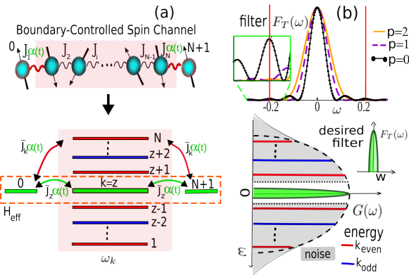
Figure 1: (Color online) (a) Top: State transfer through a spin-channel with boundary-controlled couplings. Bottom: Boundary-controlled spin chain mapped to a non-interacting spinless fermionic system (dashed rectangle) which couples to the bath fermionic-modes $k$ (red even $k$ and blue odd $k$ lines) with strengths $\tilde{J}_{k}\alpha(t)$. The two boundary spins 0 and $N+1$ are resonantly coupled to the chain by the fermionic-mode $z$ with a coupling strength $\tilde{J}_{z}\alpha(t)$ (green lines). (b) Bottom: Interacting bath-spectrum $G_{\pm}(\omega)$ including noise effects (grey color) bounded by the Wigner-semicircle (maximal-disorder) lineshape (dashed contour) with a central gap around $\omega_{z}$. In the central gap, an optimal spectral-filter $F_{T,\pm}(\omega)$ is shown (green color). Top: $F_{T,-}(\omega)$ generated by boundary-control $\alpha_{p}(t)$: $p=0\mbox{ (black dotted), $p=1$(violet dashed), }p=2$ (orange thin). The red vertical lines are the nearest bath-spectrum eigenenergies. The inset is a zoom on the tails of the filter spectrum that protects the state transfer against a general noisy bath with a central gap.

1.3 Fidelity derivation

We are interested in transferring a qubit state $|\psi_{0}\rangle$ initially stored on the $0$ qubit to the $N+1$ qubit . Here $|\psi_{0}\rangle$ is an arbitrary normalized superposition of the spin-down $|0_{0}\rangle$ and spin-up $|1_{0}\rangle$ (single-spin) states. To assess the state transfer over time $T$, we calculate the averaged fidelity $F(T)=\frac{f_{0,N+1}^{2}(T)}{6}+\frac{f_{0,N+1}(T)}{3}+\frac{1}{2}$ [3], which is the state-transfer fidelity averaged over all possible input states $|\psi_{0}\rangle$. In the interaction picture, $f_{0,N+1}(T)=\left|{}_{S}\left\langle\psi\right|\rho_{S}(T)\left|\psi\right\rangle_{S}\right|$ where $|\psi\rangle_{S}=|1_{0}\rangle\otimes|0_{z}0_{N+1}\rangle{}_{S}$ and $|\psi\rangle_{S}\otimes|\psi\rangle_{B}$ is the initial state of $S+B$.

In the ideal regime of an isolated 3-level system, perfect state transfer occurs when the accumulated phase due to the modulation control

$$\phi(T)=\tilde{J_{z}}\int_{0}^{T}\alpha(t)dt$$ (11)

satisfies $\phi(T)=\frac{\pi}{\sqrt{2}}$. Obviously, this condition does not strictly hold when the system-bath interaction is accounted for, yet it is still adequate within the second-order approximation in $H_{SB}$ used in Eq. (9). In this approximation, $f_{0,N+1}(T)$ takes the form

$$f_{0,N+1}(T)=1-\zeta(T),$$ (12)

where

$$\zeta(T)=\Re\int_{0}^{T}\!\!dt\!\int_{0}^{t}\!dt^{\prime}\binrel@{\sum}\binrel@@{\mathop{\kern 0.0pt\sum}\limits_{\pm}}\Omega_{\pm}(t)\Omega_{\pm}(t^{\prime})\Phi_{\pm}(t-t^{\prime})).$$ (13)

Here, $\Phi_{\pm}(t)=\sum_{k\in k{}_{odd(even)}}|\tilde{J}_{k}|^{2}e^{-i\omega_{k}t}$ are the bath-correlation functions, while $\Omega_{+}(t)=\alpha(t)cos(\sqrt{2}\phi(t))$ and $\Omega_{-}(t)=\alpha(t)$ are the corresponding dynamical-control functions (A-B). In the calculations we considered $|\psi\rangle_{B}=|0\rangle_{B}$. However, in the weak-coupling regime the transfer fidelity remains the same for a completely unpolarized state [65, 44] or any other initial state [25] of the bath.

In the energy domain, Eq. (13) has the convolutionless form [48, 49, 50, 51, 52, 53, 54]

$$\zeta(T)=\int_{-\infty}^{\infty}d\omega\binrel@{\sum}\binrel@@{\mathop{\kern 0.0pt\sum}\limits_{\pm}}F_{T,\pm}(\omega)G_{\pm}(\omega),$$ (14)

where the Fourier-transforms

$$G_{\pm}(\omega)=\frac{1}{2\pi}\int_{-\infty}^{\infty}dt\Phi_{\pm}(t)e^{i\omega t},\>F_{T,\pm}(\omega)=\frac{1}{2\pi}|\int_{0}^{T}dt\Omega_{\pm}(t)e^{i\omega t}|^{2}$$ (15)

are the bath-correlation spectra, $G_{\pm}(\omega)$, associated with odd(even) parity modes and the spectral filter functions, $F_{T,\pm}(\omega)$, which can be designed by the modulation control.

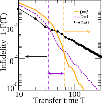
Figure 2: (Color online) Infidelity $1-F(T)$ as a function of transfer time $T$ under optimal control $\alpha_{p}(t)$: $p=0\mbox{ (black dotted), $p=1$(violet dashed), }p=2$ (orange thin), when the noise or bath-correlation spectrum $G(\omega)$ is bounded by the Wigner-semicircle with a central gap around $\omega_{z}$ (C).

2 Optimization method

To ensure the best possible state-transfer fidelity, we use modulation as a tool to minimize the infidelity $\zeta(T)$ in (13-14) by rendering the overlap between the interacting bath- and filter-spectrum functions as small as possible [46, 47].

2.1 Optimizing the modulation control for non-Markovian baths

The minimization of $\zeta(T)$ in (13) can be done for a specific bath-correlation function of a given channel which represents a non-Markovian bath. The Euler-Lagrange (E-L) equation for minimizing $\zeta(T)$ with the energy constraint

$$E(T)=\tilde{J}_{z}^{2}\int_{0}^{T}|\alpha(t)|^{2}dt$$ (16)

turns out to be

$$\frac{d}{dt}(\frac{\partial\zeta}{\partial\dot{\phi}}-\lambda\frac{\partial E}{\partial\dot{\phi}})-(\frac{\partial\zeta}{\partial\phi}-\lambda\frac{\partial E}{\partial\phi})=0,$$ (17)

where $\lambda$ is the Lagrange multiplier and $\dot{\phi}=\tilde{J_{z}}\alpha$. The optimal modulation can be obtained by solving the integro-differential equation

$$\begin{array}[]{cc}\ddot{\phi}(t)&=\frac{\sqrt{E}Q(t,\phi(t),\dot{\phi}(t))}{\tilde{J}_{z}\sqrt{\int_{0}^{T}dt\left|\int_{0}^{t}dt^{\prime}Q(t^{\prime},\phi(t^{\prime}),\dot{\phi}(t^{\prime}))\right|^{2}}},\end{array}$$ (18)

where

$$\begin{array}[]{l}Q(t,\phi(t),\dot{\phi}(t))=\int_{0}^{T}dt^{\prime}\Theta(t-t^{\prime})\frac{\dot{\phi}(t^{\prime})}{2\tilde{J}_{z}^{4}}\!\left(\frac{d\Phi_{+}(t-t^{\prime})}{dt}cos(\sqrt{2}\phi(t))cos(\sqrt{2}\phi(t^{\prime}))+\frac{d\Phi_{-}(t-t^{\prime})}{dt}\right)\\ \;\;\;\;\;\;\;\;\;\;\;\;\;\;\;\;\;\;\;\;\;\;\;\;\;\;\;+\frac{\dot{\phi}(t)}{2\tilde{J}_{z}^{4}}\left(\Phi_{+}(0)cos^{2}(\sqrt{2}\phi(t))+\Phi_{-}(0)\right).\end{array}$$ (19)

The solution of Eq. (18) should satisfy the boundary conditions $\phi(0)=0$ and $\phi(T)=\frac{\pi}{\sqrt{2}}$ to ensure the required state transfer.

In general the bath-correlations have recurrences and time fluctuations due to mesoscopic revivals in finite-length channels. Therefore, it is not trivial to solve Eqs. (18-19) analytically rather than solving them numerically for each specific channel. We however are interested in obtaining universal analytical solutions for state-transfer in the presence of non-Markovian noise sources. To this end, we here discuss suitable criteria for optimizing the state transfer in such cases.

We require the channel to be symmetric with respect to the source and target qubits and the number of eigenvalues to be odd. These requirements allow for a central eigenvalue that is invariant under noise on the couplings. This holds provided a gap exists between the central eigenvalue and the adjacent ones, i.e. they are not strongly blurred (mixed) by the noise, so as not to make them overlap. At the same time, we assume that the discreteness of the bath spectrum of the quantum channel is smoothed out by the noise, since it tends to affect more strongly the higher frequencies [34, 36, 37]. Then, if we consider the central eigenvalue as part of the system, a common characteristic of $G_{\pm}(\omega)$ is to have a central gap (as exemplified in Fig. 1b).

Therefore, in order to minimize the overlap between $G_{\pm}(\omega)$ and $F_{T,\pm}(\omega)$ for general gapped baths, and thereby the transfer infidelity in (14), we will design a narrow bandpass filter centered on the gap.

We present a universal approach that allows us to obtain analytical solutions for a narrow bandpass filter around $\omega_{z}$. Since $G_{-}(\omega)$ has a narrower gap than $G_{+}(\omega)$, we optimize the filter $F_{T,-}(\omega)$ under the variational E-L method. We seek a narrow bandpass filter, whose form on time-domain via Fourier-transform decays as slowly as possible, so as to filter out the higher frequencies. This amounts to maximizing

$$F_{T,-}(\tau)=\int_{-\infty}^{\infty}F_{T,-}(\omega)e^{-i\omega\tau}d\omega=\int_{0}^{T}\alpha(t)\alpha(t+\tau)dt,$$ (20)

subject to the variational E-L equation (17), upon replacing $\zeta$ by $F_{T,-}$. Since there is no explicit dependence on $\phi$, the second term therein is null, $\frac{\partial}{\partial\phi}(F_{T,-}-\lambda_{E}E)=0$, yielding

$$\alpha(t+\tau)+\alpha(t-\tau)=\lambda_{E}\alpha(t)+\lambda_{\phi},$$ (21)

where $\lambda_{E}$ is the Lagrange multiplier and $\lambda_{\phi}$ is an integration constant chosen to satisfy the boundary conditions obeyed by the accumulated phase (11).

Analytical solutions of (21) are obtainable for small $\tau$, corresponding to the differential equation

$$\binrel@{\alpha}\binrel@@{\mathop{\kern 0.0pt\alpha}\limits^{..}}(t)=-\tilde{\lambda}_{E}\alpha(t)+\tilde{\lambda}_{\phi},$$ (22)

with $\tilde{\lambda}_{E}=\frac{-(\lambda_{E}-2)}{\tau^{2}}$ and $\tilde{\lambda}_{\phi}=\frac{\lambda_{\phi}}{\tau^{2}}$ . It has a general solution

$$\alpha(t)=Asin(\omega_{v}t)+Bcos(\omega_{v}t)+C.$$ (23)

The unknown parameters are then optimized under chosen constraints, e.g. on the boundary coupling, the transfer time, the energy, etc.

The frequencies $\omega_{v}$ that give a low and flat filter $F_{T,-}(\omega)$ outside a small range around $\omega=\omega_{z}=0$ are $\omega_{v}=\frac{\pi n}{T}$, $n\epsilon\mathbb{Z}$, since the components of $\alpha(t)$ that oscillate with $\omega_{v}$ then interfere destructively. Only if $n=0,1,2$ will the filter have a single central peak around $\omega=0$, and the contribution of larger frequencies will be suppressed, while the filter-overlap with the central energy level will be maximized; for larger $n$, the central peak splits and additional peaks appear at larger frequencies.

Therefore, the analytical expressions for the optimal solutions satisfying $\phi(0)=0$ and $\phi(T)=\frac{\pi}{\sqrt{2}}$ are found to be

$$\alpha_{p}(t)=\alpha_{M}sin^{p}\left(\frac{\pi t}{T}\right),$$ (24)

where $p=0,1,2$,

$$\alpha_{M}=c_{p}\frac{\pi}{\sqrt{2}\tilde{J}_{z}T}$$ (25)

and $c_{p}=\frac{\sqrt{\pi}\Gamma(\frac{1+p}{2})}{\Gamma(\frac{1+p}{2})}(c_{0}=1,\,c_{1}=\frac{\pi}{2},\,c_{2}=2)$. Here $p=0$ means static control, while $p=1,2$ stand for dynamical control. Note that $T$ and $\alpha_{M}=max\{\alpha_{p}(t)\}$ cannot be independently chosen. If the transfer time is fixed, then the maximum amplitude depends on $p$, $\alpha_{M}=\alpha_{M_{p}}$, according to Eq. (25). Similarly, if the maximum amplitude is kept constant, then the transfer time will depend on $p$, $T=T_{p}$, by Eq. (25).

The different solutions in Eq. (24) are sinc-like bandpass filter functions around $0$ that become narrower as $T$ increases. For $p=0$, which satisfies the minimal-energy condition $E_{min}(T_{0})=\frac{\pi^{2}}{2T_{0}}$, the corresponding filter is the narrowest around $0$, but it has many wiggles on the filter tails (Fig. 1b) which overlap with bath-energies that hamper the transfer. In contrast, the $p=1,2$ bandpass filters are wider (for the same $T$) and require more energy, $E_{1}=\frac{\pi^{2}}{8}E_{{\scriptstyle min}}$ and $E_{2}=\frac{3}{2}E_{min}$ respectively, but these filters are flatter and lower throughout the bath-energy domain.

Hence, the bandpass filter width (i.e. full width at half maximum) and the overlap of its tail-wiggles with bath-energies as a function of $T$, determine which modulations $\alpha_{p}(t)$ are optimal, as shown in the inset of Fig. 1b ($F_{T,+}(\omega)$ filters out a similar spectral range). The shorter $T$, the lower is $p$ that yields the highest fidelity, because the central peak of the filter that produces the dominant overlap with the bath spectrum is then the narrowest. However, as $T$ increases, larger $p$ will give rise to higher fidelity, because now the tails of the filter make the dominant contribution to the overlap. As shown in Fig. 2, the filter for $p=1,2$ can improve the transfer fidelity by orders of magnitude in a noisy gapped bath bounded by the Wigner-semicircle, which is representative of fully randomized channels [66] (C).

2.2 Optimizing the modulation control for a Markovian Bath

We next consider the worst-case scenario of a Markovian bath, where the bath-correlation functions $\Phi_{\pm}(\tau)$ vanish for $\tau>0$. This is the case when the gap is closed by a noise causing the bath energy levels to fluctuate faster than the system dynamics. We note that, finding optimal solutions for the noise spectrum of a Markovian bath is important for the case where the gap is reduced or even lost in static cases.

The infidelity function (13) that must be minimized when the correlation time $\tau_{c}=0$, i.e. $\Phi_{\pm}(\tau)=\delta(\tau)$, is

$$\zeta(T)=\Re\int_{0}^{T}dt\frac{\dot{\phi}^{2}(t)}{\tilde{J}_{z}^{2}}\bigl{(}\Phi_{+}(0)cos^{2}(\sqrt{2}\phi(t))+\Phi_{-}(0)\bigr{)}.$$ (26)

The E-L equation under energy constraint (17), is now

$$\ddot{\phi}(t)\!\left(\Phi_{+}(0)cos^{2}(\sqrt{2}\phi(t))\!+\!\Phi_{-}(0)\!-\!2\lambda\tilde{J}_{z}^{2}\right)\!-\!\sqrt{2}\dot{\phi}^{2}(t)\,\Phi_{+}(0)cos(\sqrt{2}\phi(t))sin(\sqrt{2}\phi(t))\!=\!0.$$ (27)

This equation has a non-trivial analytical solution and the modulation that minimizes $\zeta(T)$ is given by the following transcendental equation

$${\normalcolor\begin{array}[]{c}T\intop_{0}^{\phi(t)}\sqrt{cos(2\sqrt{2}\phi)\Phi_{+}(0)+\Phi_{+}(0)+2\Phi_{-}(0)-2\lambda\tilde{J}_{z}^{2}}d\phi\\ -t\intop_{0}^{\phi(T)}\sqrt{2(\Phi_{+}(0)cos^{2}(\sqrt{2}\phi)+\Phi_{-}(0)-\lambda\tilde{J}_{z}^{2})}d\phi=0.\end{array}}$$ (28)

The infidelity for this optimal modulation almost coincides with the one obtained for static control ($\alpha_{p=0}(t)=\alpha_{M}$ from Eq. (24)), i.e.

$$1-F(T)\approx\frac{\pi^{2}N}{6\sqrt{2}JT}(1-\frac{\pi^{2}N}{16\sqrt{2}JT}),\>T=\frac{\pi\sqrt{N}}{2\alpha_{M}J},$$ (29)

and they only differ by about 0.1%. This optimal modulation can be phenomenologically approximated by

$$\alpha(t)\approx a\alpha_{M}+b\,sin^{q}(\frac{t\pi}{T})),\>q\sim 3.5,\>\frac{b}{a}\sim\frac{1}{3},\>a\sim 0.84,$$ (30)

assuming no constraints ($\lambda=0$). An example of the performance of this solution is discussed below and shown in Fig. 5.

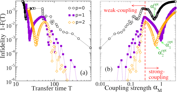
Figure 3: (Color online) Transfer infidelity $1-F(T)$ for a modulated boundary-controlled coupling $\alpha_{p}(t)=\alpha_{M}sin^{p}(\frac{\pi t}{T})$ as a function of (a) the transfer time $T$, (b) the maximum value of the boundary coupling $\alpha_{M}$: $p=0$ (empty circles), $p=1$ (filled squares), $p=2$ control (empty diamonds). The quantum channel is a homogeneous spin-chain with $N+2=31$ spins and $J=1$.

3 Optimal control of transfer in a homogeneous spin-chain channel

Consider a uniform (homogeneous) spin-chain channel, i.e. $J_{i}\equiv J$ in Eq. (1), whose energy eigenvalues are $\omega_{k}=2Jcos(\frac{k\pi}{N+1})$ [38]. In Fig. 3, we show the performance of the general optimal solutions (24) for this specific channel as a function of $\alpha_{M}$ and $T$.

The approach based on Eq. (13) strictly holds in the weak-coupling regime $(\alpha_{M}\ll 1)$ [46, 47, 48, 49, 50, 53, 54]. In this regime (marked with arrows in Fig. 3b), we found that the transfer time is $T_{p}\!\approx\!c_{p}\frac{\pi\sqrt{N}}{2\alpha_{M}J}$, and the infidelity decreases by reducing $\alpha_{M}$ according to a power law, aside from the oscillations due to the discrete nature of the bath-spectrum (see C). The filter tails are sinc-like functions, so that when a zero of the filter matches a bath-energy eigenvalue, the infidelity exhibits a dip. Aside from oscillations, the best tradeoff between speed and fidelity within this regime is given by the optimal modulation with $p=2$ (for the system described in Fig. 3a).

However, this approach can also be extended to strong couplings $\alpha_{M}$, since it becomes compatible with the weak-coupling regime under the optimal filtering process that increases the state fidelity in the interaction picture [51, 62, 63]. The bandpass filter width increases as $T$ decreases; consequently, in the strong coupling regime $(\alpha_{M}\sim 1)$ the filter may now overlap the bath energies closest to $\omega_{z}$, but still block the higher bath energies, which are the most detrimental for the state transfer [34, 36, 37]. Then, the participation of the closest bath energies yields a transfer time $T_{p}\!\approx\!c_{p}\frac{N}{2J}$. There is a clear minimal infidelity value at the point that we denote as $\alpha_{M_{p}}^{opt}$ which depends on $p$ (Fig. 3b); thus extending the previous static-control ($p=0$) results, where an optimal $\alpha_{M_{0}}^{opt}$ was found [26, 67, 68, 36]. The infidelity dip corresponds to a better filtering-out (suppression) of the higher energies, retaining only those that correspond to an almost equidistant spectrum of $\omega_{k}$ around $\omega_{z}$, which allow for coherent transfer [36].

Figure 3b shows that by fixing $\alpha_{M}$, the dynamical control ($p=1,2$) of the boundary-couplings reduces the transfer infidelity by orders of magnitude only at the expense of slowing down the transfer time $T_{p}$ at most by a factor of 2, $\frac{T_{p}}{T_{0}}\approx\frac{c_{p}}{c_{0}}\leq 2$. If the constraint on $\alpha_{M}$ can be relaxed, i.e. more energy can be used, the advantages of dynamical control can be even more appreciated for both infidelity decrease and transfer-time reduction by orders of magnitude, as shown in Fig. 3a. Hence, our main result is that the speed-fidelity tradeoff can be drastically improved under optimal dynamical control.

4 Robustness against different noises

We now explicitly consider the effects of optimal control on noise affecting the coupling strengths, also called off-diagonal noise, causing: $J_{i}\rightarrow J_{i}+J_{i}\Delta_{i}(t),\;i=1,...,N$ with $\Delta_{i}$ being a uniformly distributed random variable in the interval $\left[-\varepsilon_{J},\varepsilon_{J}\right]$. Here $\varepsilon_{J}>0$ characterizes the noise or disorder strength. When $\Delta_{i}$ is time-independent, it is called static noise, as was considered in other state-transfer protocols [69, 70, 34, 36]. When $\Delta_{i}(t)$ is time-dependent, we call it fluctuating noise [71]. These kinds of noises will affect the bath energy levels, while the central energy $\omega_{z}$ remains invariant [34, 37]. In the following we analyse the performance of the control solutions obtained in Sec. 2 for these types of noise and later on, in Sec. 4.4 we discuss briefly the effects of other sources of noise.

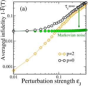
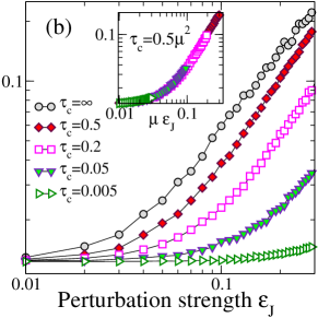
Figure 4: (Color online) Transfer infidelity for a modulated boundary-controlled coupling $\alpha_{p}(t)$ as a function of the perturbation strength $\varepsilon_{J}$ of the noisy homogeneous channel, averaged over $N_{av}$ noise realizations for (a) static and fluctuating noisy channels $\alpha_{M_{0}}^{opt}=0.6$, $\alpha_{M_{2}}^{opt}=0.7$ and $N_{av}=10^{3}$. In static noisy channels, the infidelity obtained under static control $p=0$ (empty circles) is shown to be strongly reduced when dynamical $p=2$ control is applied (empty squares). A fluctuating noisy channel is less damaging; in the Markovian limit, where the correlation time of the noise fluctuations $\tau_{c}\rightarrow 0$ ($p=0$, green solid circles), the infidelity converges to its unperturbed value. The homogeneous channel has $N+2=31$ spins and $J=1$. (b) Same plot for fluctuating noise, ranging between static and Markovian noise for $\alpha_{M_{0}}=0.1$, $T=88$ and $N_{av}=200$. Here $\tau_{c}$ is the correlation time of the noise fluctuations (see text). Faster fluctuations reduce the noise effect and thereby the fidelity decay. The inset shows the scaling of the infidelity, where the effective noise strength is scaled with $\mu=\sqrt{2\tau_{c}}$ (all curves overlap). The scaled noise strength depends on the noise correlation time $\tau_{c}$.

4.1 Static noise

Static control on the boundary-couplings can suppress static noise [34, 36] but here we show that dynamical boundary-control makes the channel even more robust, because it filters out the bath-energies that damage the transfer. To illustrate this point, we compare the effect of modulations $\alpha_{p}(t)$ with $\alpha_{M}=\alpha_{M_{p}}^{opt}$ for $p=0$ and 2 in the strong-coupling regime (Fig. 4a). There is an evident advantage of dynamical control with $p=2$ compared to static control ($p=0$), at the expense of increasing the transfer time by only a factor of 2, $\frac{T_{2}}{T_{0}}\approx 2$. In the weak-coupling regime, if we choose $\alpha_{M}$ such that the transfer fidelity is similar for $p=0$ and $p=2$, then both cases are similarly robust under static disorder, but the modulated case $p=2$ is an order of magnitude faster. Remarkably, because of disorder-induced localization [72, 73, 74, 75], regardless of how small is $\alpha_{M}$, the averaged fidelity under static noise cannot be improved beyond the bound

$$1-\bar{F}\propto N\varepsilon_{J}^{2},\>(\varepsilon_{J}\ll 1).$$ (31)

4.2 Markovian noise

The worst scenario for quantum state transfer is the absence of an energy gap around $\omega_{z}$. This case corresponds to Markovian noise characterized by $\left\langle\Delta_{i}(t)\Delta_{i}(t+\tau)\right\rangle=\delta(\tau)$, where the brackets denote the noise ensemble average, or equivalent to a bath correlation-function that vanishes at $\tau>0$. In this case there is an analytical solution for the optimal modulation given by Eq. (28), although the infidelity achieved by it almost coincides with the one obtained by the static ($p=0$) optimal control (Fig. 5). Counterintuitively, arbitrarily high fidelities can be achieved for such noise by decreasing $max\left|\alpha(t)\right|$ and thereby slowing down the transfer. This comes about because in a Markovian bath, the very fast coupling fluctuations suppress the disorder-localization effects that hamper the transfer fidelity as we show below for a typical case.

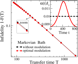
Figure 5: (Color online) Transfer infidelity as a function of the transfer time $T$ for the optimal control solution in the case of a Markovian bath (Eq. (28)) and without modulation ($p=0$). $N+2=31$, $J_{1}=J_{N}$. The corresponding boundary-couplings for $T=860$ are shown in the inset.

4.3 Non-Markovian noise

We now consider a non-Markovian noise of the form $J_{i}+J_{i}\Delta_{i}(t)$, where $\Delta_{i}(t)=\Delta_{i}\left(\left[t/\tau_{c}\right]\right)$, where the integer part $\left[t/\tau_{c}\right]=n$ defines a noise $\Delta_{i}\left(n\right)$ that randomly varies between the interval $\left[-\varepsilon_{J},\varepsilon_{J}\right]$ at time-intervals of $\tau_{c}$ during the transfer. We observe a convergence of the transfer fidelity to its value without noise as the noise correlation time $\tau_{c}$ decreases (Fig. 4b). Consequently the fidelity can be substantially improved by reducing $\alpha_{M}$. The effective noise strength scales down as $\tau_{c}^{1/2}$ (Fig. 4b, inset). By contrast to the Markovian limit $\tau_{c}\rightarrow 0$, dynamical control can strongly reduce the infidelity in the non-Markovian regime that lies between the static and Markovian limits and whose bath-spectrum is gapped.

4.4 Other sources of noise

Timing errors: In addition to resilience to noise affecting the spin-spin couplings, there is another important characteristic of the transfer robustness, namely, the length of the time window in which high fidelity is obtained. The fidelity $F(t)$ under optimal dynamical control ($p=1,2)$, yields a wider time-window around $T$ where the fidelity remains high compared with its static ($p=0)$ counterpart. This allows more time for determining the transferred state or using it for further processing. Consequently, the robustness against timing imperfections [29, 34] is increased under optimal dynamical control.

On-site energy noise: This kind of noise, alias diagonal-noise, can be either static or fluctuating. The static one can give rise to the emergence of quasi-degenerate central states. Then, the dynamical control approach introduced in this work is still capable of isolating the “system” defined here (Sec. 1) from the remaining “bath” levels. It may happen that the spin network is not symmetric with respect to the source and target spins, and then the effective couplings of the source and target qubits with the central level will not be symmetric. This asymmetry can be effectively eliminated by boundary control. On the other hand, a fluctuating diagonal-noise that may produce a fluctuation of the central energy level is here fought by optimizing the tradeoff between speed and fidelity as detailed above. Additional dynamical control of only the source and target spins can be applied to avoid these decoherence effects, by the mapping to an effective 3-level system, as a variant of dynamical decoupling [56, 57, 58, 59].

5 Conclusions

We have proposed a general, optimal dynamical control of the tradeoff between the speed and fidelity of qubit-state transfer through the central-energy global mode of a quantum channel in the presence of either static or fluctuating noise. Dynamical boundary-control has been used to design an optimal spectral filter realizable by universal, simple, modulation shapes. The resulting transfer infidelity and/or transfer time can be reduced by orders of magnitude, while their robustness against noise on the spin-spin couplings is maintained or even improved. Transfer-speed maximization is particularly important in our strive to reduce the random phase accumulated during the transfer when energy fluctuations (diagonal noise) affect the spins [76]. We have shown that, counterintuitively, static noise is more detrimental than fluctuating noise on the spin-spin couplings. This general approach is applicable to quantum channels that can be mapped to Hamiltonians quadratic in bosonic or fermionic operators [15, 16, 12, 44, 77]. We note that our control is complementary to the recently suggested control aimed at balancing possible asymmetric detunings of the boundary qubits from the channel resonance [76, 77].

Appendix A The Hamiltonian in the interaction picture

The system-bath Hamiltonian (Eq. (7) of the main text) splits into a sum of symmetric and antisymmetric system operators that are coupled to odd- and even-bath modes: $H_{SB}(t)=\binrel@{\binrel@{\sum}\binrel@@{\mathop{\kern 0.0pt\sum}\limits^{4}}}\binrel@@{\mathop{\kern 0.0pt\binrel@{\sum}\binrel@@{\mathop{\kern 0.0pt\sum}\limits^{4}}}\limits_{j=1}}\tilde{S}_{j}\otimes\tilde{B}_{j}^{\dagger},$ where $\tilde{S}_{1(3)}=\alpha(t)(c_{0}+(-)c_{N+1})$, $\tilde{S}_{2(4)}=\tilde{S}_{1(3)}^{\dagger}$, $\tilde{B}_{1(3)}=\binrel@{\sum}\binrel@@{\mathop{\kern 0.0pt\sum}\limits_{k\in k_{odd(even)}}}\tilde{J}_{k}b_{k}$ and $\tilde{B}_{2(4)}=\tilde{B}_{1(3)}^{\dagger}$. In the interaction picture $H_{SB}(t)$ becomes

$$H_{SB}^{I}(t)=\sum_{j=1}^{4}S_{j}(t)\otimes B_{j}^{\dagger}(t),$$ (32)

where

$$\begin{array}[]{c}S_{j}(t)=U_{S}^{\dagger}(t)\tilde{S}_{j}(t)U_{S}(t),\,U_{S}(t)=\mathcal{T}e^{-i\intop_{0}^{t}dt^{{}^{\prime}}H_{S}(t^{{}^{\prime}})},\\ B_{j}(t)=U_{B}^{\dagger}(t)\tilde{B}_{j}U_{B}(t),\,U_{B}(t)=e^{-iH_{B}t};\end{array}$$ (33)

and the evolution operators are

$$\begin{array}[]{l}\begin{array}[]{cl}U_{S}(t)=&|0\rangle_{SS}\langle 0|+\left(\frac{\cos(\sqrt{2}\phi(t))+1}{2}\right)\left(|0\rangle\langle 0|+|N+1\rangle\langle N+1|\right)\\ &+\left(\frac{\cos(\sqrt{2}\phi(t))-1}{2}\right)\left(|0\rangle\langle N+1|+|N+1\rangle\langle 0|\right)\\ &+\cos(\sqrt{2}\phi(t))|z\rangle\langle z|-i\,\frac{\sin(\sqrt{2}\phi(t))}{2}\left(|0\rangle\langle z|+|N+1\rangle\langle z|+h.c.\right),\\ U_{B}(t)=&\binrel@{\binrel@{\sum}\binrel@@{\mathop{\kern 0.0pt\sum}\limits_{k=1,k\neq z}}}\binrel@@{\mathop{\kern 0.0pt\binrel@{\sum}\binrel@@{\mathop{\kern 0.0pt\sum}\limits_{k=1,k\neq z}}}\limits^{N}}e^{-i\omega_{k}t}|k\rangle\langle k|+|0\rangle_{BB}\langle 0|,\end{array}\end{array}$$ (34)

where the states $|0\rangle_{S}=|0_{0}0_{z}0_{N+1}\rangle_{S}$ and $|0\rangle_{B}=|0_{1}...0_{N}\rangle_{B}$ refer to the zero-excitation states in the system (S) and bath (B) respectively. Therefore, the bath operators are $B_{1(3)}(t)=\binrel@{\sum}\binrel@@{\mathop{\kern 0.0pt\sum}\limits_{k\in k_{odd(even)}}}|\tilde{J}_{k}|^{2}e^{-i\omega_{k}t}|k\rangle{}_{B}\langle 0|,\,B_{2(4)}(t)=B_{1(3)}^{\dagger}(t)$.

We define a basis of operators $\hat{\nu}_{i}$ to describe the rotating system operators $S_{j}(t)$ via a rotation-matrix $\Omega_{j,i}(t)$. They are given by

$$\begin{array}[]{cc}\hat{\nu}_{1}=|0\rangle_{S}\left(\langle 0|+\langle N+1|\right)&\hat{\nu}_{2}=\hat{\nu}_{1}^{\dagger},\\ \hat{\nu}_{3}=|0\rangle_{S}\langle z|&\hat{\nu}_{4}=\hat{\nu}_{3}^{\dagger},\\ \hat{\nu}_{5}=|0\rangle_{S}\left(\langle 0|-\langle N+1|\right)&\hat{\nu}_{6}=\hat{\nu}_{5}^{\dagger},\end{array}$$ (35)

such that $S_{j}(t)=\binrel@{\binrel@{\sum}\binrel@@{\mathop{\kern 0.0pt\sum}\limits_{i=1}}}\binrel@@{\mathop{\kern 0.0pt\binrel@{\sum}\binrel@@{\mathop{\kern 0.0pt\sum}\limits_{i=1}}}\limits^{6}}\Omega_{j,i}(t)\hat{\nu}_{i}.$ Given that $S_{1}(t)=\dot{\phi}(t)\left(cos(\sqrt{2}\phi(t))\hat{\nu}_{1}-i\,\sqrt{2}sin(\sqrt{2}\phi(t))\hat{\nu}_{3}\right)$, $S_{3}(t)=\dot{\phi}(t)\hat{\nu}_{5},\,S_{2(4)}(t)=S_{1(3)}^{\dagger}(t)$ the rotation-matrix vectors are

$$\begin{array}[]{c}\begin{array}[]{l}\Omega_{1,i}(t)=\dot{\phi}(t)\left(cos(\sqrt{2}\phi(t)),0,-i\,\sqrt{2}sin(\sqrt{2}\phi(t)),0,0,0\right)\\ \Omega_{2,i}(t)=\dot{\phi}(t)\left(0,cos(\sqrt{2}\phi(t)),0,i\,\sqrt{2}sin(\sqrt{2}\phi(t)),0,0\right)\\ \Omega_{3,i}(t)=\dot{\phi}(t)(0,0,0,0,1,0)\\ \Omega_{4,i}(t)=\dot{\phi}(t)(0,0,0,0,0,1).\end{array}\end{array}$$ (36)

Appendix B The fidelity in the interaction picture

Here we derive Eqs. (12-13) from Eq. (9) of the main text. Considering $|\psi\rangle=|100...0\rangle_{SB}=|\psi\rangle_{S}\otimes|0\rangle_{B}$ with $|\psi\rangle_{S}=|1_{0}0_{z}0_{N+1}\rangle_{S}$ as the initial state, the fidelity is reduced to

$$\begin{array}[]{cc}f_{0,N+1}(T)=&\left|{}_{S}\left\langle\psi\right|\rho_{S}(T)\left|\psi\right\rangle_{S}\right|=1-\zeta(T)\end{array},$$ (37)

where $\zeta(T)=T\binrel@{\binrel@{\sum}\binrel@@{\mathop{\kern 0.0pt\sum}\limits^{6}}}\binrel@@{\mathop{\kern 0.0pt\binrel@{\sum}\binrel@@{\mathop{\kern 0.0pt\sum}\limits^{6}}}\limits_{i,i^{\prime}=1}}R_{i,i^{\prime}}(T)\Gamma_{i,i^{{}^{\prime}}}$, with

$$\Gamma_{i,i^{{}^{\prime}}}={}_{S}\left\langle\psi\right|[\hat{\nu}_{i},\hat{\nu}_{i^{\prime}}\left|\psi\right\rangle_{S}{}_{S}\left\langle\psi\right|]\left|\psi\right\rangle_{S}=\delta_{i,2}\delta_{1,i^{\prime}}+\delta_{i,2}\delta_{5,i^{\prime}}+\delta_{i,6}\delta_{1,i^{\prime}}+\delta_{i,6}\delta_{5,i^{\prime}}$$ (38)

and

$$R_{i,i^{\prime}}(T)\!=\!\frac{1}{T}\int_{0}^{T}dt\!\int_{0}^{t}dt^{\prime}(\Phi_{2,1}(t-t^{\prime})\Omega_{2,i}(t)\Omega_{1,i^{\prime}}(t^{\prime})+\Phi_{4,3}(t-t^{\prime})\Omega_{4,i}(t)\Omega_{3,i^{\prime}}(t^{\prime})).$$ (39)

Here $\hat{\nu}_{i^{\prime}}$ and $\Omega_{j,i}$ are as defined in Eqs. (35-36), while the correlation functions are

$$\Phi_{j,j^{\prime}}(t-t^{\prime})=\sum_{k\in k_{odd}}|\tilde{J}_{k}|^{2}e^{-i\omega_{k}(t-t^{\prime})}\delta_{j,2}\delta_{1,j^{\prime}}+\sum_{k\in k_{even}}|\tilde{J}_{k}|^{2}e^{-i\omega_{k}(t-t^{\prime})}\delta_{j,4}\delta_{3,j^{\prime}}.$$ (40)

This leads to the infidelity $\zeta(T)$ of Eq. (13).

Appendix C Considerations for a specific non-Markovian bath: the uniform spin-channel

Consider a uniform (homogeneous) spin-chain channel, i.e. $J_{i}\equiv J$ in Eq.(1), whose energy eigenvalues are $\omega_{k}=2Jcos(\frac{k\pi}{N+1})$. In the weak-coupling regime where $\alpha_{M}\ll 1$, the coupling strength in the interaction $H_{bc}$, $\tilde{J}_{z}=\sqrt{\frac{2}{N+1}}J$ and $\tilde{J}_{k}=\tilde{J}_{z}sin(\frac{k\pi}{N+1})$, are always much smaller than the nearest eigenvalue gap $|\omega_{z}-\omega_{z\pm 1}|\sim\frac{2J}{N}$ [38, 39, 44]. The correlation function of the bath is

$$\Phi_{\pm}(\tau)=\binrel@{\sum}\binrel@@{\mathop{\kern 0.0pt\sum}\limits_{k{}_{odd(even)}}}\left|\sqrt{\frac{2}{N\!+\!1}}Jsin(\frac{k\pi}{N\!+\!1})\right|^{2}e^{-i2Jcos(\frac{k\pi}{N+1})\tau}$$ (41)

and has recurrences and time fluctuations due to mesoscopic revivals, while at short times $t$, it behaves as a Bessel function ${\color[rgb]{0,0,0}{\color[rgb]{1,0,0}{\color[rgb]{0,0,0}\Phi(t)=\frac{2(\alpha_{0}J)^{2}}{J\tau}\mathtt{\mathcal{J}_{1}(}2Jt)}}}$. The latter correlation function represents the limiting case of an infinite channel and it gives a continuous bath-spectrum that becomes a semicircle. In the case of a finite channel, $G(\omega)$ will be discrete but modulated by the semicircle with a central gap. If disorder is considered, the position of the spectrum lines fluctuates from channel to channel but they are essentially modulated by the semicircle with a central gap as was considered in the Fig. 1b of the main text, where

$$G_{\pm}(\omega)=\frac{1}{2}\sqrt{4J^{2}-\omega^{2}}(1-\Theta(\omega-\omega_{l})\Theta(\omega+\omega_{l})),\>\omega_{l}=\frac{3\omega_{z+1}}{4}.$$ (42)

This is the Wigner-distribution for fully randomized channels [66] with a central gap.

References

References

- [1] Ernst Ising. Beitrag zur theorie des ferromagnetismus. Z. Phys., 31(1):253–258, February 1925.
- [2] B Kramer and A MacKinnon. Localization: theory and experiment. Rep. Prog. Phys., 56(12):1469–1564, December 1993.
- [3] Sougato Bose. Quantum Communication through an Unmodulated Spin Chain. Phys. Rev. Lett., 91:207901, November 2003.
- [4] Sougato Bose. Contemporary Physics, 48(1):13–30, 2007.
- [5] A. Lyakhov and C. Bruder. Quantum state transfer in arrays of flux qubits. New J. Phys., 7:181, August 2005.
- [6] J. Majer, J. M. Chow, J. M. Gambetta, Jens Koch, B. R. Johnson, J. A. Schreier, L. Frunzio, D. I. Schuster, A. A. Houck, A. Wallraff, A. Blais, M. H. Devoret, S. M. Girvin, and R. J. Schoelkopf. Coupling superconducting qubits via a cavity bus. Nature, 449(7161):443–447, September 2007.
- [7] L.-M. Duan, E. Demler, and M. D. Lukin. Controlling Spin Exchange Interactions of Ultracold Atoms in Optical Lattices. Phys. Rev. Lett., 91(9):090402, August 2003.
- [8] Michael J. Hartmann, Fernando G. S. L. Brandao, and Martin B. Plenio. Effective Spin Systems in Coupled Microcavities. Phys. Rev. Lett., 99(16):160501, October 2007.
- [9] Takeshi Fukuhara, Adrian Kantian, Manuel Endres, Marc Cheneau, Peter Schauß, Sebastian Hild, David Bellem, Ulrich Schollwöck, Thierry Giamarchi, Christian Gross, Immanuel Bloch, and Stefan Kuhr. Quantum dynamics of a mobile spin impurity. Nat. Phys., 9(4):235–241, April 2013.
- [10] Jonathan Simon, Waseem S. Bakr, Ruichao Ma, M. Eric Tai, Philipp M. Preiss, and Markus Greiner. Quantum simulation of antiferromagnetic spin chains in an optical lattice. Nature, 472(7343):307–312, April 2011.
- [11] Z. L. Mádi, B. Brutscher, T. Schulte-Herbruggen, R. Bruschweiler, and R. R. Ernst. Time-resolved observation of spin waves in a linear chain of nuclear spins. Chem. Phys. Lett., 268(3-4):300–305, April 1997.
- [12] S. Doronin, I. Maksimov, and E. Feldman. Multiple-quantum dynamics of one-dimensional nuclear spin systems in solids. J. Exp. Theor. Phys., 91(3):597, 2000.
- [13] Jingfu Zhang, Gui Lu Long, Wei Zhang, Zhiwei Deng, Wenzhang Liu, and Zhiheng Lu. Simulation of Heisenberg XY interactions and realization of a perfect state transfer in spin chains using liquid nuclear magnetic resonance. Phys. Rev. A, 72(1):012331, July 2005.
- [14] Jingfu Zhang, Nageswaran Rajendran, Xinhua Peng, and Dieter Suter. Iterative quantum-state transfer along a chain of nuclear spin qubits. Phys. Rev. A, 76(1):012317, July 2007.
- [15] P. Cappellaro, C. Ramanathan, and D. G. Cory. Dynamics and control of a quasi-one-dimensional spin system. Phys. Rev. A, 76(3):032317, 2007.
- [16] E. Rufeil-Fiori, C. M. Sánchez, F. Y. Oliva, H. M. Pastawski, and P. R. Levstein. Effective one-body dynamics in multiple-quantum NMR experiments. Phys. Rev. A, 79(3):032324, March 2009.
- [17] Gonzalo A. Álvarez, Mor Mishkovsky, Ernesto P. Danieli, Patricia R. Levstein, Horacio M. Pastawski, and Lucio Frydman. Perfect state transfers by selective quantum interferences within complex spin networks. Phys. Rev. A, 81(6):060302 (R), June 2010.
- [18] Ashok Ajoy, Rama Koteswara Rao, Anil Kumar, and Pranaw Rungta. Algorithmic approach to simulate hamiltonian dynamics and an NMR simulation of quantum state transfer. Phys. Rev. A, 85(3):030303, March 2012.
- [19] D. Petrosyan and P. Lambropoulos. Coherent population transfer in a chain of tunnel coupled quantum dots. Opt. Commun., 264(2):419–425, August 2006.
- [20] B. P. Lanyon, C. Hempel, D. Nigg, M. Müller, R. Gerritsma, F. Zähringer, P. Schindler, J. T. Barreiro, M. Rambach, G. Kirchmair, M. Hennrich, P. Zoller, R. Blatt, and C. F. Roos. Universal digital quantum simulation with trapped ions. Science, 334(6052):57–61, October 2011.
- [21] R. Blatt and C. F. Roos. Quantum simulations with trapped ions. Nat. Phys., 8(4):277–284, April 2012.
- [22] P. Cappellaro, L. Jiang, J. S. Hodges, and M. D. Lukin. Coherence and Control of Quantum Registers Based on Electronic Spin in a Nuclear Spin Bath. Phys. Rev. Lett., 102(21):210502, May 2009.
- [23] P. Neumann, R. Kolesov, B. Naydenov, J. Beck, F. Rempp, M. Steiner, V. Jacques, G. Balasubramanian, M. L. Markham, D. J. Twitchen, S. Pezzagna, J. Meijer, J. Twamley, F. Jelezko, and J. Wrachtrup. Quantum register based on coupled electron spins in a room-temperature solid. Nat. Phys., 6(4):249–253, April 2010.
- [24] N. Y. Yao, L. Jiang, A. V. Gorshkov, P. C. Maurer, G. Giedke, J. I. Cirac, and M. D. Lukin. Scalable architecture for a room temperature solid-state quantum information processor. Nat. Commun., 3:800, April 2012.
- [25] Yuting Ping, Brendon W. Lovett, Simon C. Benjamin, and Erik M. Gauger. Practicality of spin chain wiring in diamond quantum technologies. Phys. Rev. Lett., 110(10):100503, March 2013.
- [26] Analia Zwick and Omar Osenda. Quantum state transfer in a XX chain with impurities. J. Phys. A: Math. Theor., 44:5302, March 2011.
- [27] Matthias Christandl, Nilanjana Datta, Tony C. Dorlas, Artur Ekert, Alastair Kay, and Andrew J. Landahl. Perfect transfer of arbitrary states in quantum spin networks. Phys. Rev. A, 71(3):032312, March 2005.
- [28] Peter Karbach and Joachim Stolze. Spin chains as perfect quantum state mirrors. Phys. Rev. A, 72:30301 (R), September 2005.
- [29] Alastair Kay. Perfect state transfer: Beyond nearest-neighbor couplings. Phys. Rev. A, 73:32306, March 2006.
- [30] Alastair Kay. Perfect, efficient, state transfer and its application as a constructive tool. Int. J. of Quantum Inform., 08(04):641–676, 2010.
- [31] Matthias Christandl, Nilanjana Datta, Artur Ekert, and Andrew J. Landahl. Perfect state transfer in quantum spin networks. Phys. Rev. Lett., 92:187902, May 2004.
- [32] Claudio Albanese, Matthias Christandl, Nilanjana Datta, and Artur Ekert. Mirror inversion of quantum states in linear registers. Phys. Rev. Lett., 93:230502, Nov 2004.
- [33] C. Di Franco, M. Paternostro, and M. S. Kim. Perfect state transfer on a spin chain without state initialization. Phys. Rev. Lett., 101:230502, Dec 2008.
- [34] Analia Zwick, Gonzalo A. Álvarez, Joachim Stolze, and Omar Osenda. Robustness of spin-coupling distributions for perfect quantum state transfer. Phys. Rev. A, 84:22311, August 2011.
- [35] Gonzalo A. Álvarez and Dieter Suter. NMR quantum simulation of localization effects induced by decoherence. Phys. Rev. Lett., 104(23):230403, June 2010.
- [36] Analia Zwick, Gonzalo A. Álvarez, Joachim Stolze, and Omar Osenda. Spin chains for robust state transfer: Modified boundary couplings versus completely engineered chains. Phys. Rev. A, 85(1):012318, January 2012.
- [37] Joachim Stolze, Gonzalo A. Álvarez, Omar Osenda, and Analia Zwick. Robustness of spin-chain state-transfer schemes. In Georgios M. Nikolopoulos and Igor Jex, editors, Quantum State Transfer and Quantum Network Engineering, Quantum Science and Technology Series. Springer, Berlin, 2014.
- [38] Antoni Wojcik, Tomasz Luczak, Pawel Kurzynski, Andrzej Grudka, Tomasz Gdala, and Malgorzata Bednarska. Unmodulated spin chains as universal quantum wires. Phys. Rev. A, 72(3):034303, 2005.
- [39] Antoni Wojcik, Tomasz Luczak, Pawel Kurzynski, Andrzej Grudka, Tomasz Gdala, and Malgorzata Bednarska. Multiuser quantum communication networks. Phys. Rev. A, 75(2):022330, February 2007.
- [40] L. Campos Venuti, C. Degli Esposti Boschi, and M. Roncaglia. Qubit teleportation and transfer across antiferromagnetic spin chains. Phys. Rev. Lett., 99:060401, Aug 2007.
- [41] L. Campos Venuti, S. M. Giampaolo, F. Illuminati, and P. Zanardi. Long-distance entanglement and quantum teleportation in xx spin chains. Phys. Rev. A, 76:052328, Nov 2007.
- [42] Salvatore M. Giampaolo and Fabrizio Illuminati. Long-distance entanglement and quantum teleportation in coupled-cavity arrays. Phys. Rev. A, 80:050301, Nov 2009.
- [43] Salvatore M Giampaolo and Fabrizio Illuminati. Long-distance entanglement in many-body atomic and optical systems. New Journal of Physics, 12(2):025019, 2010.
- [44] N. Y. Yao, L. Jiang, A. V. Gorshkov, Z.-X. Gong, A. Zhai, L.-M. Duan, and M. D. Lukin. Robust Quantum State Transfer in Random Unpolarized Spin Chains. Phys. Rev. Lett., 106:40505, January 2011.
- [45] Henry L. Haselgrove. Optimal state encoding for quantum walks and quantum communication over spin systems. Phys. Rev. A, 72:062326, Dec 2005.
- [46] Jens Clausen, Guy Bensky, and Gershon Kurizki. Bath-Optimized Minimal-Energy Protection of Quantum Operations from Decoherence. Phys. Rev. Lett., 104(4):040401, January 2010.
- [47] Jens Clausen, Guy Bensky, and Gershon Kurizki. Task-optimized control of open quantum systems. Phys. Rev. A, 85(5):052105, May 2012.
- [48] B. M. Escher, G. Bensky, J. Clausen, and G. Kurizki. Optimized control of quantum state transfer from noisy to quiet qubits. J. Phys. B: At. Mol. Opt. Phys., 44(15):154015, August 2011.
- [49] Guy Bensky, David Petrosyan, Johannes Majer, Jörg Schmiedmayer, and Gershon Kurizki. Optimizing inhomogeneous spin ensembles for quantum memory. Phys. Rev. A, 86(1):012310, July 2012.
- [50] David Petrosyan, Guy Bensky, Gershon Kurizki, Igor Mazets, Johannes Majer, and Jörg Schmiedmayer. Reversible state transfer between superconducting qubits and atomic ensembles. Phys. Rev. A, 79(4):040304, April 2009.
- [51] Goren Gordon, Noam Erez, and Gershon Kurizki. Universal dynamical decoherence control of noisy single- and multi-qubit systems. J. Phys. B: At. Mol. Opt. Phys., 40(9):S75, May 2007.
- [52] Goren Gordon, Gershon Kurizki, and Daniel A. Lidar. Optimal Dynamical Decoherence Control of a Qubit. Phys. Rev. Lett., 101(1):010403, July 2008.
- [53] A. G. Kofman and G. Kurizki. Universal Dynamical Control of Quantum Mechanical Decay: Modulation of the Coupling to the Continuum. Phys. Rev. Lett., 87(27):270405, December 2001.
- [54] A. G. Kofman and G. Kurizki. Unified Theory of Dynamically Suppressed Qubit Decoherence in Thermal Baths. Phys. Rev. Lett., 93(13):130406, September 2004.
- [55] Lian-Ao Wu, Gershon Kurizki, and Paul Brumer. Master equation and control of an open quantum system with leakage. Phys. Rev. Lett., 102(8):080405, February 2009.
- [56] Lorenza Viola and Seth Lloyd. Dynamical suppression of decoherence in two-state quantum systems. Phys. Rev. A, 58:2733–2744, Oct 1998.
- [57] Lorenza Viola, Emanuel Knill, and Seth Lloyd. Dynamical decoupling of open quantum systems. Physical Review Letters, 82(12):2417, March 1999.
- [58] Lorenza Viola and Emanuel Knill. Robust dynamical decoupling of quantum systems with bounded controls. Phys. Rev. Lett., 90:037901, Jan 2003.
- [59] K. Khodjasteh and D. A. Lidar. Fault-tolerant quantum dynamical decoupling. Phys. Rev. Lett., 95:180501, Oct 2005.
- [60] Elliott Lieb, Theodore Schultz, and Daniel Mattis. Two soluble models of an antiferromagnetic chain. Ann. Phys., 16(3):407–466, December 1961.
- [61] Goren Gordon and Gershon Kurizki. Scalability of decoherence control in entangled systems. Phys. Rev. A, 83(3):032321, March 2011.
- [62] Goren Gordon. Dynamical decoherence control of multi-partite systems. J. Phys. B: At. Mol. Opt. Phys., 42(22):223001, November 2009.
- [63] Gershon Kurizki. Universal dynamical control of open quantum systems. ISRN Optics, 2013:783865, 2013.
- [64] P. Rebentrost, I. Serban, T. Schulte-Herbrüggen, and F. K. Wilhelm. Optimal control of a qubit coupled to a non-markovian environment. Phys. Rev. Lett., 102:090401, Mar 2009.
- [65] Ernesto P. Danieli, Horacio M. Pastawski, and Gonzalo A. Álvarez. Quantum dynamics under coherent and incoherent effects of a spin bath in the keldysh formalism: application to a spin swapping operation. Chem. Phys. Lett., 402(1):88, January 2005.
- [66] Eugene P. Wigner. On the distribution of the roots of certain symmetric matrices. Ann. Math., 67(2):325–327, March 1958.
- [67] L. Banchi, T. J. G. Apollaro, A. Cuccoli, R. Vaia, and P. Verrucchi. Long quantum channels for high-quality entanglement transfer. New J. Phys., 13(12):123006, December 2011.
- [68] L. Banchi, T. J. G. Apollaro, A. Cuccoli, R. Vaia, and P. Verrucchi. Optimal dynamics for quantum-state and entanglement transfer through homogeneous quantum systems. Phys. Rev. A, 82(5):052321, November 2010.
- [69] Gabriele de Chiara, Davide Rossini, Simone Montangero, and Rosario Fazio. From perfect to fractal transmission in spin chains. Phys. Rev. A, 72:12323, July 2005.
- [70] R. Ronke, T. P. Spiller, and I. D’Amico. Effect of perturbations on information transfer in spin chains. Phys. Rev. A, 83:12325, January 2011.
- [71] D. Burgarth. Quantum state transfer and time-dependent disorder in quantum chains. The European Physical Journal Special Topics, 151(1):147–155, 2007.
- [72] Charles E. Porter. Statistical Theories of Spectra Fluctuations: a Collection of Reprints and Original Papers. Acad. Press., 1965.
- [73] Yoseph Imry. Introduction to Mesoscopic Physics. Oxford University Press, 2001.
- [74] V.M Akulin and G Kurizki. Spectral lines of symmetrically shaped particles or clusters with internal disorder. Phys. Lett. A, 174(3):267–272, March 1993.
- [75] S. Pellegrin, A. Kozhekin, A. Sarfati, V. M. Akulin, and G. Kurizki. Mie resonance in dielectric droplets with internal disorder. Phys. Rev. A, 63(3):033814, February 2001.
- [76] Ashok Ajoy and Paola Cappellaro. Perfect quantum transport in arbitrary spin networks. Phys. Rev. B, 87:064303, Feb 2013.
- [77] N. Y. Yao, Z.-X. Gong, C. R. Laumann, S. D. Bennett, L.-M. Duan, M. D. Lukin, L. Jiang, and A. V. Gorshkov. Quantum logic between remote quantum registers. Phys. Rev. A, 87:022306, Feb 2013.