A link between microstructure evolution and macroscopic response in elasto-plasticity: formulation and numerical approximation of the higher-dimensional Continuum Dislocation Dynamics theory

Abstract

Micro-plasticity theories and models are suitable to explain and predict mechanical response of devices on length scales where the influence of the carrier of plastic deformation – the dislocations – cannot be neglected or completely averaged out. To consider these effects without resolving each single dislocation a large variety of continuum descriptions has been developed, amongst which the higher-dimensional continuum dislocation dynamics (hdCDD) theory by Hochrainer et al. (Phil. Mag. 87, pp. 1261-1282) takes a different, statistical approach and contains information that are usually only contained in discrete dislocation models. We present a concise formulation of hdCDD in a general single-crystal plasticity context together with a discontinuous Galerkin scheme for the numerical implementation which we evaluate by numerical examples: a thin film under tensile and shear loads. We study the influence of different realistic boundary conditions and demonstrate that dislocation fluxes and their lines’ curvature are key features in small-scale plasticity.

url]http://www.matsim.techfak.uni-erlangen.de

1 Introduction

Plastic deformation of metals has been utilized by man since the copper age and the knowledge of how to process metals (by e.g. forging) has constantly grown. However, the physical mechanisms underlying the empirical procedures could not be understood until the crystalline structure of metals was investigated by Rutherford at the beginning of the 20th century. Subsequent attempts to explain the discrepancy between the theoretically predicted shear strength of a metal and the experimentally observed yield stresses lead to the concept of the ‘dislocation’ – a linear crystal defect – which was proposed in the 1930s independently by Orowan (1934), Polanyi (1934) and Taylor (1934a). Two decades later Kondo (1952), Nye (1953), Bilby et al. (1955) and Kröner (1958) independently introduced equivalent measures for the average plastic deformation state of a crystal in the form of a second-rank dislocation density tensor. This ’Kröner-Nye tensor’ is introduced to link the microscopically discontinuous to a macroscopically continuous deformation state and is the fundamental quantity in Kröner’s continuum theory of dislocations. It has been used widely until today (see e.g. the related works in Acharya and Fressengeas (2012); Taupin et al. (2013); Le and Günther (2014)). This tensor, however, only captures inhomogeneous plastic deformation states associated with so-called geometrically necessary dislocations (GNDs) and does not account for the accumulation of so-called statistically stored dislocations (SSDs) in homogeneous plasticity. This limits the applicability of the classical dislocation density measure within continuum theories of plasticity.

Phenomenological continuum models for plasticity which are not based on dislocation mechanics have been successful in a wide range of engineering applications. They operate on length scales where the properties of materials and systems are scale invariant. The scale-invariance, however, breaks down at dimensions below a few micro-meters, which is also a scale of growing technological interest. These microstructural effects become more and more pronounced in small systems and lead to so-called ’size effects’ (e.g. Ashby, 1970; Arzt, 1998; Stolken and Evans, 1998; Greer and De Hosson, 2011). Phenomenological continuum theories incorporate internal length scales by introducing strain gradient terms – sometimes based on the consideration of GND densities – into their constitutive equations (e.g. Fleck et al., 1994; Nix and Gao, 1998; Gurtin, 2002; Gao and Huang, 2003; Zhang et al., 2014) but are not able to consider fluxes of dislocations or the conversion of SSDs into GNDs and vice versa. Refined continuum formulations (with or without strain gradients) include additional information in a mechanism-based approach (Engels et al., 2012; Li et al., 2014) or take multi-scale approaches by directly including information from lower scale models (Wallin et al., 2008; Xiong et al., 2012).

Discrete dislocation dynamics (DDD) models (e.g. Kubin and Canova, 1992; Devincre and Kubin, 1997; Fivel et al., 1997; Ghoniem et al., 2000; Weygand et al., 2002; Bulatov and Cai, 2002; Arsenlis et al., 2007; Zhou et al., 2010; Po et al., 2014) contain very detailed information about the dislocation microstructure and the interaction and evolution of dislocations and have been successful over the last two decades in predicting plasticity at the micro-meter scale. DDD simulations allow to investigate complex plastic deformation mechanisms but are, however, due to their high computational cost limited to small system sizes/small densities.

A different approach which is closely related to DDD and which generalizes the classical continuum theory of dislocations was undertaken by Groma et al. (Groma, 1997; Groma et al., 2003). They used methods from statistical physics to describe systems of positive and negative straight edge dislocations in analogy to densities of charged point particles. The resulting evolution equations are able to faithfully describe fluxes of signed edge dislocations and the conversion of SSDs into GNDs (and vice versa). This approach has been successfully used by a number of groups (e.g. Yefimov et al., 2004; Kratochvil et al., 2007; Hirschberger et al., 2011; Scardia et al., 2014). A generalization to systems of curved dislocation loops, however, is not straightforward. Pioneering steps into that direction have been undertaken by Kosevich (1979); El-Azab (2000); Sedláček et al. (2003). Furthermore, ’screw-edge’ representations have been introduced as an approximation by Arsenlis et al. (2004); Zaiser and Hochrainer (2006); Reuber et al. (2014) and Leung et al. (2015); Xiang and co-workers developed a model for the evolution of curved systems of geometrically necessary dislocations (Xiang, 2009). Their model also includes line tension effects and was e.g. applied to model Frank-Read sources (Zhu et al., 2014). A new approach based on statistical averages of differential geometrical formulations of dislocation lines has been done by Hochrainer (Hochrainer, 2006; Hochrainer et al., 2007; Sandfeld et al., 2010) who generalized the statistical approach of Groma towards systems of dislocations with arbitrary line orientation and line curvature introducing the higher-dimensional Continuum Dislocation Dynamics (hdCDD) theory. The key idea of hdCDD is based on mapping spatial, parameterized dislocation lines into a higher-dimensional configuration space, which contains the local line orientation as additional information. This is particularly useful in situations with complex microstructure (Sandfeld et al., 2010, 2015). In order to avoid the high computational cost of the higher-dimensional configuration space, ’integrated’ variants of hdCDD – denoted by CDD – have also been developed recently and their simplifying assumptions already have been benchmarked for a number of situation (Hochrainer et al., 2009; Sandfeld et al., 2011; Hochrainer et al., 2014; Zaiser and Sandfeld, 2014; Monavari et al., 2014). Furthermore, very recently one CDD variant has been coupled to a strain gradient plasticity model (Wulfinghoff and Böhlke, 2015) and was used to study size effects of a composite material. Until now hdCDD nonetheless serves as reference method for all CDD formulations, since it can be considered as an almost exact continuum representation of ensembles of curved dislocations and allows to access many relevant microstructural information.

In this article, we derive and formulate the governing equations for hdCDD in a general crystal plasticity context. We start by introducing the formulation for single-crystal plasticity and the elasto-plastic boundary value problem and connect this to the dislocation system in a staggered scheme. The evolution of the dislocation density and the dislocation curvature density is computed in representative slip planes depending on the dislocation velocity. This is approximated by a discontinuous Galerkin (DG) scheme introduced in Sect. 3 with a local Fourier ansatz suitable for the higher dimensional configuration space. Numerical examples in Sect. 4 – tension and shearing of a thin film – demonstrate the influence of passivated and non-passivated surfaces on the microstructure evolution. Furthermore we study the influence of the lines’ curvature on the plastic deformation behavior and also on the stress-strain response of the specimen and compare with the formulation of Groma.

2 Crystal elasto-plasticity based on the hdCDD theory

In this section we introduce the elastic eigenstrain problem and its variational formulation (Sect. 2.1 and Sect. 2.2) and two different models for representing slip planes (Sect. 2.3) in a continuum framework. Then we outline the hdCDD theory extending the classical quantities from Kröner’s continuum theory: the governing equations for the evolution of dislocation density and curvature density as defined by the higher dimensional continuum dislocation dynamics theory are introduced in Sect. 2.5; our model for the dislocation velocity governing the dislocation dynamics is determined by the constitutive setting explained in Sect. 2.7.

2.1 A continuum model for single-crystal plasticity

Let the reference configuration $\mathcal{B}$ be a bounded Lipschitz domain in $\mathbb{R}^{3}$ and let $\partial_{\text{D}}\mathcal{B}\cup\partial_{\text{N}}\mathcal{B}=\partial\mathcal{B}$ be a non-overlapping decomposition into Dirichlet boundary $\partial_{\text{D}}\mathcal{B}$ and Neumann boundary $\partial_{\text{N}}\mathcal{B}$. The position of a material point is denoted by $\textstyle\mathbf{x}$ and the displacement of the body from its reference configuration by $\mathchoice{\mbox{\boldmath$\displaystyle\mathbf{u}$}}{\mbox{\boldmath$\textstyle\mathbf{u}$}}{\mbox{\boldmath$\scriptstyle\mathbf{u}$}}{\mbox{\boldmath$\scriptscriptstyle\mathbf{u}$}}(\mathchoice{\mbox{\boldmath$\displaystyle\mathbf{x}$}}{\mbox{\boldmath$\textstyle\mathbf{x}$}}{\mbox{\boldmath$\scriptstyle\mathbf{x}$}}{\mbox{\boldmath$\scriptscriptstyle\mathbf{x}$}},t)$. The distortion tensor

$$\mathrm{D}\mathchoice{\mbox{\boldmath$\displaystyle\mathbf{u}$}}{\mbox{\boldmath$\textstyle\mathbf{u}$}}{\mbox{\boldmath$\scriptstyle\mathbf{u}$}}{\mbox{\boldmath$\scriptscriptstyle\mathbf{u}$}} = \mathchoice{\mbox{\boldmath$\displaystyle\mathbf{\beta}$}}{\mbox{\boldmath$\textstyle\mathbf{\beta}$}}{\mbox{\boldmath$\scriptstyle\mathbf{\beta}$}}{\mbox{\boldmath$\scriptscriptstyle\mathbf{\beta}$}}^{\text{el}}+\mathchoice{\mbox{\boldmath$\displaystyle\mathbf{\beta}$}}{\mbox{\boldmath$\textstyle\mathbf{\beta}$}}{\mbox{\boldmath$\scriptstyle\mathbf{\beta}$}}{\mbox{\boldmath$\scriptscriptstyle\mathbf{\beta}$}}^{\text{pl}}$$ (1)

is decomposed additively into elastic and plastic parts $\mathchoice{\mbox{\boldmath$\displaystyle\mathbf{\beta}$}}{\mbox{\boldmath$\textstyle\mathbf{\beta}$}}{\mbox{\boldmath$\scriptstyle\mathbf{\beta}$}}{\mbox{\boldmath$\scriptscriptstyle\mathbf{\beta}$}}^{\text{el}}$ and $\mathchoice{\mbox{\boldmath$\displaystyle\mathbf{\beta}$}}{\mbox{\boldmath$\textstyle\mathbf{\beta}$}}{\mbox{\boldmath$\scriptstyle\mathbf{\beta}$}}{\mbox{\boldmath$\scriptscriptstyle\mathbf{\beta}$}}^{\text{pl}}$, respectively. Small deformations are assumed so that the infinitesimal strain is given by

$$\mathchoice{\mbox{\boldmath$\displaystyle\mathbf{\varepsilon}$}}{\mbox{\boldmath$\textstyle\mathbf{\varepsilon}$}}{\mbox{\boldmath$\scriptstyle\mathbf{\varepsilon}$}}{\mbox{\boldmath$\scriptscriptstyle\mathbf{\varepsilon}$}}=\mathchoice{\mbox{\boldmath$\displaystyle\mathbf{\varepsilon}$}}{\mbox{\boldmath$\textstyle\mathbf{\varepsilon}$}}{\mbox{\boldmath$\scriptstyle\mathbf{\varepsilon}$}}{\mbox{\boldmath$\scriptscriptstyle\mathbf{\varepsilon}$}}(\mathchoice{\mbox{\boldmath$\displaystyle\mathbf{u}$}}{\mbox{\boldmath$\textstyle\mathbf{u}$}}{\mbox{\boldmath$\scriptstyle\mathbf{u}$}}{\mbox{\boldmath$\scriptscriptstyle\mathbf{u}$}})=\operatorname*{sym}(\mathrm{D}\mathchoice{\mbox{\boldmath$\displaystyle\mathbf{u}$}}{\mbox{\boldmath$\textstyle\mathbf{u}$}}{\mbox{\boldmath$\scriptstyle\mathbf{u}$}}{\mbox{\boldmath$\scriptscriptstyle\mathbf{u}$}})\,.$$ (2)

Plastic slip is assumed to take place on $N$ slip systems determined by a unit normal $\mathchoice{\mbox{\boldmath$\displaystyle\mathbf{m}$}}{\mbox{\boldmath$\textstyle\mathbf{m}$}}{\mbox{\boldmath$\scriptstyle\mathbf{m}$}}{\mbox{\boldmath$\scriptscriptstyle\mathbf{m}$}}_{s}$ and slip direction $\mathchoice{\mbox{\boldmath$\displaystyle\mathbf{d}$}}{\mbox{\boldmath$\textstyle\mathbf{d}$}}{\mbox{\boldmath$\scriptstyle\mathbf{d}$}}{\mbox{\boldmath$\scriptscriptstyle\mathbf{d}$}}_{s}=\frac{1}{b_{s}}\mathchoice{\mbox{\boldmath$\displaystyle\mathbf{b}$}}{\mbox{\boldmath$\textstyle\mathbf{b}$}}{\mbox{\boldmath$\scriptstyle\mathbf{b}$}}{\mbox{\boldmath$\scriptscriptstyle\mathbf{b}$}}_{s}$ on the $s$-th system, where $\mathchoice{\mbox{\boldmath$\displaystyle\mathbf{b}$}}{\mbox{\boldmath$\textstyle\mathbf{b}$}}{\mbox{\boldmath$\scriptstyle\mathbf{b}$}}{\mbox{\boldmath$\scriptscriptstyle\mathbf{b}$}}_{s}$ is the Burgers vector of length $b_{s}=|\mathchoice{\mbox{\boldmath$\displaystyle\mathbf{b}$}}{\mbox{\boldmath$\textstyle\mathbf{b}$}}{\mbox{\boldmath$\scriptstyle\mathbf{b}$}}{\mbox{\boldmath$\scriptscriptstyle\mathbf{b}$}}_{s}|$. As an example, the face-centered cubic (FCC) crystal has $N=12$ slip systems. In special situations symmetry can be exploited and the case $N=1$ or $N=2$ can be considered over the crystal of thin film via shearing and bending situations.

The plastic shear strain in the slip system $s$ is denoted by $\gamma_{s}$. In the single crystal, we assume that the plastic part of the displacement gradient is given by the sum over the contributions from all active slip systems

$$\mathchoice{\mbox{\boldmath$\displaystyle\mathbf{\beta}$}}{\mbox{\boldmath$\textstyle\mathbf{\beta}$}}{\mbox{\boldmath$\scriptstyle\mathbf{\beta}$}}{\mbox{\boldmath$\scriptscriptstyle\mathbf{\beta}$}}^{\text{pl}} = \sum\nolimits_{s}\gamma_{s}\mathchoice{\mbox{\boldmath$\displaystyle\mathbf{M}$}}{\mbox{\boldmath$\textstyle\mathbf{M}$}}{\mbox{\boldmath$\scriptstyle\mathbf{M}$}}{\mbox{\boldmath$\scriptscriptstyle\mathbf{M}$}}_{s}$$ (3)

where $\mathchoice{\mbox{\boldmath$\displaystyle\mathbf{M}$}}{\mbox{\boldmath$\textstyle\mathbf{M}$}}{\mbox{\boldmath$\scriptstyle\mathbf{M}$}}{\mbox{\boldmath$\scriptscriptstyle\mathbf{M}$}}_{s}=\frac{1}{b_{s}}\mathchoice{\mbox{\boldmath$\displaystyle\mathbf{b}$}}{\mbox{\boldmath$\textstyle\mathbf{b}$}}{\mbox{\boldmath$\scriptstyle\mathbf{b}$}}{\mbox{\boldmath$\scriptscriptstyle\mathbf{b}$}}_{s}\otimes\mathchoice{\mbox{\boldmath$\displaystyle\mathbf{m}$}}{\mbox{\boldmath$\textstyle\mathbf{m}$}}{\mbox{\boldmath$\scriptstyle\mathbf{m}$}}{\mbox{\boldmath$\scriptscriptstyle\mathbf{m}$}}_{s}=\mathchoice{\mbox{\boldmath$\displaystyle\mathbf{d}$}}{\mbox{\boldmath$\textstyle\mathbf{d}$}}{\mbox{\boldmath$\scriptstyle\mathbf{d}$}}{\mbox{\boldmath$\scriptscriptstyle\mathbf{d}$}}_{s}\otimes\mathchoice{\mbox{\boldmath$\displaystyle\mathbf{m}$}}{\mbox{\boldmath$\textstyle\mathbf{m}$}}{\mbox{\boldmath$\scriptstyle\mathbf{m}$}}{\mbox{\boldmath$\scriptscriptstyle\mathbf{m}$}}_{s}$ is the projection tensor accounting for the orientation of the slip system $s$. Depending on the vector of plastic shear strains $\mathchoice{\mbox{\boldmath$\displaystyle\mathbf{\gamma}$}}{\mbox{\boldmath$\textstyle\mathbf{\gamma}$}}{\mbox{\boldmath$\scriptstyle\mathbf{\gamma}$}}{\mbox{\boldmath$\scriptscriptstyle\mathbf{\gamma}$}}=(\gamma_{1},\dots,\gamma_{N})^{\top}$, the plastic strain is given by

$$\mathchoice{\mbox{\boldmath$\displaystyle\mathbf{\varepsilon}$}}{\mbox{\boldmath$\textstyle\mathbf{\varepsilon}$}}{\mbox{\boldmath$\scriptstyle\mathbf{\varepsilon}$}}{\mbox{\boldmath$\scriptscriptstyle\mathbf{\varepsilon}$}}^{\text{pl}}=\mathchoice{\mbox{\boldmath$\displaystyle\mathbf{\varepsilon}$}}{\mbox{\boldmath$\textstyle\mathbf{\varepsilon}$}}{\mbox{\boldmath$\scriptstyle\mathbf{\varepsilon}$}}{\mbox{\boldmath$\scriptscriptstyle\mathbf{\varepsilon}$}}^{\text{pl}}(\mathchoice{\mbox{\boldmath$\displaystyle\mathbf{\gamma}$}}{\mbox{\boldmath$\textstyle\mathbf{\gamma}$}}{\mbox{\boldmath$\scriptstyle\mathbf{\gamma}$}}{\mbox{\boldmath$\scriptscriptstyle\mathbf{\gamma}$}})=\text{sym}(\mathchoice{\mbox{\boldmath$\displaystyle\mathbf{\beta}$}}{\mbox{\boldmath$\textstyle\mathbf{\beta}$}}{\mbox{\boldmath$\scriptstyle\mathbf{\beta}$}}{\mbox{\boldmath$\scriptscriptstyle\mathbf{\beta}$}}^{\text{pl}})=\sum\nolimits_{s}\gamma_{s}\mathchoice{\mbox{\boldmath$\displaystyle\mathbf{M}$}}{\mbox{\boldmath$\textstyle\mathbf{M}$}}{\mbox{\boldmath$\scriptstyle\mathbf{M}$}}{\mbox{\boldmath$\scriptscriptstyle\mathbf{M}$}}_{s}^{\text{sym}}\,,\qquad\mathchoice{\mbox{\boldmath$\displaystyle\mathbf{M}$}}{\mbox{\boldmath$\textstyle\mathbf{M}$}}{\mbox{\boldmath$\scriptstyle\mathbf{M}$}}{\mbox{\boldmath$\scriptscriptstyle\mathbf{M}$}}_{s}^{\text{sym}}=\operatorname*{sym}(\mathchoice{\mbox{\boldmath$\displaystyle\mathbf{M}$}}{\mbox{\boldmath$\textstyle\mathbf{M}$}}{\mbox{\boldmath$\scriptstyle\mathbf{M}$}}{\mbox{\boldmath$\scriptscriptstyle\mathbf{M}$}}_{s})\,.$$ (4)

This defines the elastic strain

$$\mathchoice{\mbox{\boldmath$\displaystyle\mathbf{\varepsilon}$}}{\mbox{\boldmath$\textstyle\mathbf{\varepsilon}$}}{\mbox{\boldmath$\scriptstyle\mathbf{\varepsilon}$}}{\mbox{\boldmath$\scriptscriptstyle\mathbf{\varepsilon}$}}^{\text{el}} = \mathchoice{\mbox{\boldmath$\displaystyle\mathbf{\varepsilon}$}}{\mbox{\boldmath$\textstyle\mathbf{\varepsilon}$}}{\mbox{\boldmath$\scriptstyle\mathbf{\varepsilon}$}}{\mbox{\boldmath$\scriptscriptstyle\mathbf{\varepsilon}$}}^{\text{el}}(\mathchoice{\mbox{\boldmath$\displaystyle\mathbf{u}$}}{\mbox{\boldmath$\textstyle\mathbf{u}$}}{\mbox{\boldmath$\scriptstyle\mathbf{u}$}}{\mbox{\boldmath$\scriptscriptstyle\mathbf{u}$}},\mathchoice{\mbox{\boldmath$\displaystyle\mathbf{\gamma}$}}{\mbox{\boldmath$\textstyle\mathbf{\gamma}$}}{\mbox{\boldmath$\scriptstyle\mathbf{\gamma}$}}{\mbox{\boldmath$\scriptscriptstyle\mathbf{\gamma}$}})\quad=\quad\mathchoice{\mbox{\boldmath$\displaystyle\mathbf{\varepsilon}$}}{\mbox{\boldmath$\textstyle\mathbf{\varepsilon}$}}{\mbox{\boldmath$\scriptstyle\mathbf{\varepsilon}$}}{\mbox{\boldmath$\scriptscriptstyle\mathbf{\varepsilon}$}}(\mathchoice{\mbox{\boldmath$\displaystyle\mathbf{u}$}}{\mbox{\boldmath$\textstyle\mathbf{u}$}}{\mbox{\boldmath$\scriptstyle\mathbf{u}$}}{\mbox{\boldmath$\scriptscriptstyle\mathbf{u}$}})-\mathchoice{\mbox{\boldmath$\displaystyle\mathbf{\varepsilon}$}}{\mbox{\boldmath$\textstyle\mathbf{\varepsilon}$}}{\mbox{\boldmath$\scriptstyle\mathbf{\varepsilon}$}}{\mbox{\boldmath$\scriptscriptstyle\mathbf{\varepsilon}$}}^{\text{pl}}(\mathchoice{\mbox{\boldmath$\displaystyle\mathbf{\gamma}$}}{\mbox{\boldmath$\textstyle\mathbf{\gamma}$}}{\mbox{\boldmath$\scriptstyle\mathbf{\gamma}$}}{\mbox{\boldmath$\scriptscriptstyle\mathbf{\gamma}$}})\,.$$ (5)

2.2 Variational balance equations

The macroscopic equilibrium equation is given by

$$-\operatorname*{div}\mathchoice{\mbox{\boldmath$\displaystyle\mathbf{\sigma}$}}{\mbox{\boldmath$\textstyle\mathbf{\sigma}$}}{\mbox{\boldmath$\scriptstyle\mathbf{\sigma}$}}{\mbox{\boldmath$\scriptscriptstyle\mathbf{\sigma}$}} = \mathchoice{\mbox{\boldmath$\displaystyle\mathbf{f}$}}{\mbox{\boldmath$\textstyle\mathbf{f}$}}{\mbox{\boldmath$\scriptstyle\mathbf{f}$}}{\mbox{\boldmath$\scriptscriptstyle\mathbf{f}$}}_{\mathcal{B}}\quad\text{ in }\,\mathcal{B}\,,$$ (6)

with the body force $\mathchoice{\mbox{\boldmath$\displaystyle\mathbf{f}$}}{\mbox{\boldmath$\textstyle\mathbf{f}$}}{\mbox{\boldmath$\scriptstyle\mathbf{f}$}}{\mbox{\boldmath$\scriptscriptstyle\mathbf{f}$}}_{\mathcal{B}}$ and the constitutive relation for the Cauchy stress tensor

$$\mathchoice{\mbox{\boldmath$\displaystyle\mathbf{\sigma}$}}{\mbox{\boldmath$\textstyle\mathbf{\sigma}$}}{\mbox{\boldmath$\scriptstyle\mathbf{\sigma}$}}{\mbox{\boldmath$\scriptscriptstyle\mathbf{\sigma}$}}=\mathbb{C}:\mathchoice{\mbox{\boldmath$\displaystyle\mathbf{\varepsilon}$}}{\mbox{\boldmath$\textstyle\mathbf{\varepsilon}$}}{\mbox{\boldmath$\scriptstyle\mathbf{\varepsilon}$}}{\mbox{\boldmath$\scriptscriptstyle\mathbf{\varepsilon}$}}^{\text{el}}=\mathbb{C}:(\mathchoice{\mbox{\boldmath$\displaystyle\mathbf{\varepsilon}$}}{\mbox{\boldmath$\textstyle\mathbf{\varepsilon}$}}{\mbox{\boldmath$\scriptstyle\mathbf{\varepsilon}$}}{\mbox{\boldmath$\scriptscriptstyle\mathbf{\varepsilon}$}}-\mathchoice{\mbox{\boldmath$\displaystyle\mathbf{\varepsilon}$}}{\mbox{\boldmath$\textstyle\mathbf{\varepsilon}$}}{\mbox{\boldmath$\scriptstyle\mathbf{\varepsilon}$}}{\mbox{\boldmath$\scriptscriptstyle\mathbf{\varepsilon}$}}^{\text{pl}})$$ (7)

depending on the elasticity tensor $\mathbb{C}$. The macroscopic boundary conditions are

$$\mathchoice{\mbox{\boldmath$\displaystyle\mathbf{u}$}}{\mbox{\boldmath$\textstyle\mathbf{u}$}}{\mbox{\boldmath$\scriptstyle\mathbf{u}$}}{\mbox{\boldmath$\scriptscriptstyle\mathbf{u}$}}=\mathchoice{\mbox{\boldmath$\displaystyle\mathbf{u}$}}{\mbox{\boldmath$\textstyle\mathbf{u}$}}{\mbox{\boldmath$\scriptstyle\mathbf{u}$}}{\mbox{\boldmath$\scriptscriptstyle\mathbf{u}$}}_{\text{D}}\ \text{ on }\ \partial_{\text{D}}\mathcal{B}, \mathchoice{\mbox{\boldmath$\displaystyle\mathbf{\sigma}$}}{\mbox{\boldmath$\textstyle\mathbf{\sigma}$}}{\mbox{\boldmath$\scriptstyle\mathbf{\sigma}$}}{\mbox{\boldmath$\scriptscriptstyle\mathbf{\sigma}$}}\mathchoice{\mbox{\boldmath$\displaystyle\mathbf{n}$}}{\mbox{\boldmath$\textstyle\mathbf{n}$}}{\mbox{\boldmath$\scriptstyle\mathbf{n}$}}{\mbox{\boldmath$\scriptscriptstyle\mathbf{n}$}}=\mathchoice{\mbox{\boldmath$\displaystyle\mathbf{g}$}}{\mbox{\boldmath$\textstyle\mathbf{g}$}}{\mbox{\boldmath$\scriptstyle\mathbf{g}$}}{\mbox{\boldmath$\scriptscriptstyle\mathbf{g}$}}_{\text{N}}\ \text{ on }\ \partial_{\text{N}}\mathcal{B}\,,$$ (8)

where $\mathchoice{\mbox{\boldmath$\displaystyle\mathbf{u}$}}{\mbox{\boldmath$\textstyle\mathbf{u}$}}{\mbox{\boldmath$\scriptstyle\mathbf{u}$}}{\mbox{\boldmath$\scriptscriptstyle\mathbf{u}$}}_{\text{D}}$ is a prescribed displacement for Dirichlet boundary and $\mathchoice{\mbox{\boldmath$\displaystyle\mathbf{g}$}}{\mbox{\boldmath$\textstyle\mathbf{g}$}}{\mbox{\boldmath$\scriptstyle\mathbf{g}$}}{\mbox{\boldmath$\scriptscriptstyle\mathbf{g}$}}_{\text{N}}$ is an applied traction for Neumann boundary. Let $U=\big{\{}\mathchoice{\mbox{\boldmath$\displaystyle\mathbf{u}$}}{\mbox{\boldmath$\textstyle\mathbf{u}$}}{\mbox{\boldmath$\scriptstyle\mathbf{u}$}}{\mbox{\boldmath$\scriptscriptstyle\mathbf{u}$}}\in\mathrm{H}^{1}(\mathcal{B},\mathbb{R}^{3})\colon\mathchoice{\mbox{\boldmath$\displaystyle\mathbf{u}$}}{\mbox{\boldmath$\textstyle\mathbf{u}$}}{\mbox{\boldmath$\scriptstyle\mathbf{u}$}}{\mbox{\boldmath$\scriptscriptstyle\mathbf{u}$}}=\mathchoice{\mbox{\boldmath$\displaystyle\mathbf{0}$}}{\mbox{\boldmath$\textstyle\mathbf{0}$}}{\mbox{\boldmath$\scriptstyle\mathbf{0}$}}{\mbox{\boldmath$\scriptscriptstyle\mathbf{0}$}}$ on $\partial_{\text{D}}\mathcal{B}\big{\}}$, and assume that $\mathchoice{\mbox{\boldmath$\displaystyle\mathbf{u}$}}{\mbox{\boldmath$\textstyle\mathbf{u}$}}{\mbox{\boldmath$\scriptstyle\mathbf{u}$}}{\mbox{\boldmath$\scriptscriptstyle\mathbf{u}$}}_{\text{D}}$ extends to $\mathcal{B}$. Then, for given $\mathchoice{\mbox{\boldmath$\displaystyle\mathbf{\varepsilon}$}}{\mbox{\boldmath$\textstyle\mathbf{\varepsilon}$}}{\mbox{\boldmath$\scriptstyle\mathbf{\varepsilon}$}}{\mbox{\boldmath$\scriptscriptstyle\mathbf{\varepsilon}$}}^{\text{pl}}=\mathchoice{\mbox{\boldmath$\displaystyle\mathbf{\varepsilon}$}}{\mbox{\boldmath$\textstyle\mathbf{\varepsilon}$}}{\mbox{\boldmath$\scriptstyle\mathbf{\varepsilon}$}}{\mbox{\boldmath$\scriptscriptstyle\mathbf{\varepsilon}$}}^{\text{pl}}(\mathchoice{\mbox{\boldmath$\displaystyle\mathbf{\gamma}$}}{\mbox{\boldmath$\textstyle\mathbf{\gamma}$}}{\mbox{\boldmath$\scriptstyle\mathbf{\gamma}$}}{\mbox{\boldmath$\scriptscriptstyle\mathbf{\gamma}$}})$ , we have in weak form: find $\mathchoice{\mbox{\boldmath$\displaystyle\mathbf{u}$}}{\mbox{\boldmath$\textstyle\mathbf{u}$}}{\mbox{\boldmath$\scriptstyle\mathbf{u}$}}{\mbox{\boldmath$\scriptscriptstyle\mathbf{u}$}}\in\mathchoice{\mbox{\boldmath$\displaystyle\mathbf{u}$}}{\mbox{\boldmath$\textstyle\mathbf{u}$}}{\mbox{\boldmath$\scriptstyle\mathbf{u}$}}{\mbox{\boldmath$\scriptscriptstyle\mathbf{u}$}}_{\text{D}}+U$ such that

$$\int_{\mathcal{B}}\big{(}\mathchoice{\mbox{\boldmath$\displaystyle\mathbf{\varepsilon}$}}{\mbox{\boldmath$\textstyle\mathbf{\varepsilon}$}}{\mbox{\boldmath$\scriptstyle\mathbf{\varepsilon}$}}{\mbox{\boldmath$\scriptscriptstyle\mathbf{\varepsilon}$}}(\mathchoice{\mbox{\boldmath$\displaystyle\mathbf{u}$}}{\mbox{\boldmath$\textstyle\mathbf{u}$}}{\mbox{\boldmath$\scriptstyle\mathbf{u}$}}{\mbox{\boldmath$\scriptscriptstyle\mathbf{u}$}})-\mathchoice{\mbox{\boldmath$\displaystyle\mathbf{\varepsilon}$}}{\mbox{\boldmath$\textstyle\mathbf{\varepsilon}$}}{\mbox{\boldmath$\scriptstyle\mathbf{\varepsilon}$}}{\mbox{\boldmath$\scriptscriptstyle\mathbf{\varepsilon}$}}^{\text{pl}}\big{)}:\mathbb{C}:\mathchoice{\mbox{\boldmath$\displaystyle\mathbf{\varepsilon}$}}{\mbox{\boldmath$\textstyle\mathbf{\varepsilon}$}}{\mbox{\boldmath$\scriptstyle\mathbf{\varepsilon}$}}{\mbox{\boldmath$\scriptscriptstyle\mathbf{\varepsilon}$}}(\delta\mathchoice{\mbox{\boldmath$\displaystyle\mathbf{u}$}}{\mbox{\boldmath$\textstyle\mathbf{u}$}}{\mbox{\boldmath$\scriptstyle\mathbf{u}$}}{\mbox{\boldmath$\scriptscriptstyle\mathbf{u}$}})\,\mathrm{d}\mathchoice{\mbox{\boldmath$\displaystyle\mathbf{x}$}}{\mbox{\boldmath$\textstyle\mathbf{x}$}}{\mbox{\boldmath$\scriptstyle\mathbf{x}$}}{\mbox{\boldmath$\scriptscriptstyle\mathbf{x}$}}=\int_{\mathcal{B}}\mathchoice{\mbox{\boldmath$\displaystyle\mathbf{f}$}}{\mbox{\boldmath$\textstyle\mathbf{f}$}}{\mbox{\boldmath$\scriptstyle\mathbf{f}$}}{\mbox{\boldmath$\scriptscriptstyle\mathbf{f}$}}_{\mathcal{B}}\cdot\delta\mathchoice{\mbox{\boldmath$\displaystyle\mathbf{u}$}}{\mbox{\boldmath$\textstyle\mathbf{u}$}}{\mbox{\boldmath$\scriptstyle\mathbf{u}$}}{\mbox{\boldmath$\scriptscriptstyle\mathbf{u}$}}\,\mathrm{d}\mathchoice{\mbox{\boldmath$\displaystyle\mathbf{x}$}}{\mbox{\boldmath$\textstyle\mathbf{x}$}}{\mbox{\boldmath$\scriptstyle\mathbf{x}$}}{\mbox{\boldmath$\scriptscriptstyle\mathbf{x}$}}+\int_{\partial_{\text{N}}\mathcal{B}}\mathchoice{\mbox{\boldmath$\displaystyle\mathbf{g}$}}{\mbox{\boldmath$\textstyle\mathbf{g}$}}{\mbox{\boldmath$\scriptstyle\mathbf{g}$}}{\mbox{\boldmath$\scriptscriptstyle\mathbf{g}$}}_{\text{N}}\cdot\delta\mathchoice{\mbox{\boldmath$\displaystyle\mathbf{u}$}}{\mbox{\boldmath$\textstyle\mathbf{u}$}}{\mbox{\boldmath$\scriptstyle\mathbf{u}$}}{\mbox{\boldmath$\scriptscriptstyle\mathbf{u}$}}\,\mathrm{d}\mathchoice{\mbox{\boldmath$\displaystyle\mathbf{a}$}}{\mbox{\boldmath$\textstyle\mathbf{a}$}}{\mbox{\boldmath$\scriptstyle\mathbf{a}$}}{\mbox{\boldmath$\scriptscriptstyle\mathbf{a}$}}\,,\qquad\delta\mathchoice{\mbox{\boldmath$\displaystyle\mathbf{u}$}}{\mbox{\boldmath$\textstyle\mathbf{u}$}}{\mbox{\boldmath$\scriptstyle\mathbf{u}$}}{\mbox{\boldmath$\scriptscriptstyle\mathbf{u}$}}\in U\,.$$ (9)

This is complemented by an evolution equation for the plastic shear strain (the Orowan relation (Orowan, 1940)) depending on the dislocation density and the dislocation velocity.

2.3 Dislocation densities, plastic shear strain, and the representation of physical slip planes

Since continuum dislocation theories operate with averaged measures one has to consider slip planes in a consistent sense (i.e., consistent with the averaging). In the slip system $s$, we use a discrete set of ’crystallographic’ slip planes (SP) of distance ${\vartriangle}s>0$

$$\Gamma_{s,g}=\big{\{}\mathchoice{\mbox{\boldmath$\displaystyle\mathbf{z}$}}{\mbox{\boldmath$\textstyle\mathbf{z}$}}{\mbox{\boldmath$\scriptstyle\mathbf{z}$}}{\mbox{\boldmath$\scriptscriptstyle\mathbf{z}$}}_{s,g}+\eta\mathchoice{\mbox{\boldmath$\displaystyle\mathbf{d}$}}{\mbox{\boldmath$\textstyle\mathbf{d}$}}{\mbox{\boldmath$\scriptstyle\mathbf{d}$}}{\mbox{\boldmath$\scriptscriptstyle\mathbf{d}$}}_{s}+\xi\mathchoice{\mbox{\boldmath$\displaystyle\mathbf{d}$}}{\mbox{\boldmath$\textstyle\mathbf{d}$}}{\mbox{\boldmath$\scriptstyle\mathbf{d}$}}{\mbox{\boldmath$\scriptscriptstyle\mathbf{d}$}}_{s}\times\mathchoice{\mbox{\boldmath$\displaystyle\mathbf{m}$}}{\mbox{\boldmath$\textstyle\mathbf{m}$}}{\mbox{\boldmath$\scriptstyle\mathbf{m}$}}{\mbox{\boldmath$\scriptscriptstyle\mathbf{m}$}}_{s}\colon(\eta,\xi)\in\mathbb{R}^{2}\big{\}}\,,$$ (10)

where $\mathchoice{\mbox{\boldmath$\displaystyle\mathbf{z}$}}{\mbox{\boldmath$\textstyle\mathbf{z}$}}{\mbox{\boldmath$\scriptstyle\mathbf{z}$}}{\mbox{\boldmath$\scriptscriptstyle\mathbf{z}$}}_{s,g}\in\Gamma_{s,g}$ denotes the origin of the local $(\eta,\xi)$ coordinate system which is aligned such that the Burgers vector $\mathchoice{\mbox{\boldmath$\displaystyle\mathbf{b}$}}{\mbox{\boldmath$\textstyle\mathbf{b}$}}{\mbox{\boldmath$\scriptstyle\mathbf{b}$}}{\mbox{\boldmath$\scriptscriptstyle\mathbf{b}$}}_{s}$ points into positive $\eta$ direction and $\xi$ points into the line direction of a positive edge dislocation; a position in the slip plane is denoted by $\mathchoice{\mbox{\boldmath$\displaystyle\mathbf{r}$}}{\mbox{\boldmath$\textstyle\mathbf{r}$}}{\mbox{\boldmath$\scriptstyle\mathbf{r}$}}{\mbox{\boldmath$\scriptscriptstyle\mathbf{r}$}}\in\Gamma_{s,g}$. Each SP is expanded to a thin layer of width $h\leq{\vartriangle}s$ (collecting a small number of physical slip planes)

$$\mathcal{B}_{s,g}=\Bigl{\{}\mathchoice{\mbox{\boldmath$\displaystyle\mathbf{z}$}}{\mbox{\boldmath$\textstyle\mathbf{z}$}}{\mbox{\boldmath$\scriptstyle\mathbf{z}$}}{\mbox{\boldmath$\scriptscriptstyle\mathbf{z}$}}\in\mathcal{B}\colon\mathchoice{\mbox{\boldmath$\displaystyle\mathbf{z}$}}{\mbox{\boldmath$\textstyle\mathbf{z}$}}{\mbox{\boldmath$\scriptstyle\mathbf{z}$}}{\mbox{\boldmath$\scriptscriptstyle\mathbf{z}$}}=\mathchoice{\mbox{\boldmath$\displaystyle\mathbf{r}$}}{\mbox{\boldmath$\textstyle\mathbf{r}$}}{\mbox{\boldmath$\scriptstyle\mathbf{r}$}}{\mbox{\boldmath$\scriptscriptstyle\mathbf{r}$}}+\zeta\mathchoice{\mbox{\boldmath$\displaystyle\mathbf{m}$}}{\mbox{\boldmath$\textstyle\mathbf{m}$}}{\mbox{\boldmath$\scriptstyle\mathbf{m}$}}{\mbox{\boldmath$\scriptscriptstyle\mathbf{m}$}}_{s}\text{ with }\mathchoice{\mbox{\boldmath$\displaystyle\mathbf{r}$}}{\mbox{\boldmath$\textstyle\mathbf{r}$}}{\mbox{\boldmath$\scriptstyle\mathbf{r}$}}{\mbox{\boldmath$\scriptscriptstyle\mathbf{r}$}}\in\Gamma_{s,g}\text{ and }|\zeta|\leq h/2\Big{\}}\,.$$ (11)

In our model, the dislocation density in the slip system $s$ is represented by the average $\rho_{s,g}$ in the layer $\mathcal{B}_{s,g}$ such that the sum of all $\rho_{s,g}$ integrated over each layer equals the total dislocation line length in $\mathcal{B}$.

Experimental observation of surface slip traces. This illustrative example shows a plastically deformed (cadmium) single crystal (height $\approx 800$µm).

. Permission granted by DoITPoMS

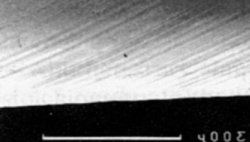
The physical model idealizes the real specimen: The ’crystallographic’ slip planes are evenly spaced with distance ${\vartriangle}s$ which is typically much smaller than the simulated distance in the numerical model below.

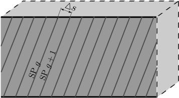
Numerical model
The ’numerical slip planes’ represent a number of physical slip planes either in a quasi-discrete setting (Case 1, left) or in a fully continuous setting (Case 2, right).

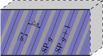
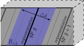
Case 1: direct SP representation     Case 2: averaged SP representation            

Figure 1: From the real system to the numerical model: representation of crystallographic slip planes for one slip system.

Since the evolution of the dislocation density $\rho_{s,g}$ and the Orowan relation of the plastic shear strain are evaluated only in the crystallographic slip planes $\Gamma_{s,g}$, the continuum approach requires to extend the values to the body $\mathcal{B}$. For this purpose, we introduce the orthogonal projection $P_{s,g}\colon\mathcal{B}\longrightarrow\Gamma_{s,g}$, and for $\mathchoice{\mbox{\boldmath$\displaystyle\mathbf{r}$}}{\mbox{\boldmath$\textstyle\mathbf{r}$}}{\mbox{\boldmath$\scriptstyle\mathbf{r}$}}{\mbox{\boldmath$\scriptscriptstyle\mathbf{r}$}}\in\Gamma_{s,g}\setminus\mathcal{B}$ the plastic shear strain $\gamma_{s,g}$ is extended by constant continuation. We consider two cases (compare Fig. 1):

Case 1: Direct representation of crystallographic SPs.

We set

$$\gamma_{s}(\mathchoice{\mbox{\boldmath$\displaystyle\mathbf{r}$}}{\mbox{\boldmath$\textstyle\mathbf{r}$}}{\mbox{\boldmath$\scriptstyle\mathbf{r}$}}{\mbox{\boldmath$\scriptscriptstyle\mathbf{r}$}}) = \begin{cases}\frac{{\vartriangle}s}{h}\gamma_{s,g}({\mathchoice{\mbox{\boldmath$\displaystyle\mathbf{r}$}}{\mbox{\boldmath$\textstyle\mathbf{r}$}}{\mbox{\boldmath$\scriptstyle\mathbf{r}$}}{\mbox{\boldmath$\scriptscriptstyle\mathbf{r}$}}})&\mathchoice{\mbox{\boldmath$\displaystyle\mathbf{r}$}}{\mbox{\boldmath$\textstyle\mathbf{r}$}}{\mbox{\boldmath$\scriptstyle\mathbf{r}$}}{\mbox{\boldmath$\scriptscriptstyle\mathbf{r}$}}\in\mathcal{B}_{s,g}\text{ for some }g\,,\\ 0&\text{else}\end{cases}$$ (12)

where the factor of ${{\vartriangle}s}/{h}$ accounts for the fact that the plastic strain will be defined for the elastic BVP only in the blue regions in Case 1. The objective of Case 1 is to analyze how to choose ${\vartriangle}s$ and $h$ for our density-based micro-structure representation. This case also serves as a reference for Case 2 and was set up following the idea of discrete dislocation dynamics simulations: for the limit $h\rightarrow 0$ we can approach a discrete SP representation; this provides benchmark data for Case 2.

Case 2: Averaged representation of crystallographic SPs.

Alternatively, we average over multiple crystallographical SPs in order to arrive at a representation of, e.g., dislocation density or plastic strain in which they are distributed field quantities – not only within the SP but also in direction of the slip system normal. Therefore, we first collapse a number of crystallographic SPs that are contained within a region of width ${\vartriangle}\overline{s}\gg h$ into one representative SP by summing up the respective dislocation field variables over ${\vartriangle}\overline{s}$. The representative SPs are numbered by $\overline{g}$. All points $\textstyle\mathbf{r}$ of this layer belong to the domain

$$\overline{\mathcal{B}}_{s,\overline{g}}=\Bigl{\{}\mathchoice{\mbox{\boldmath$\displaystyle\mathbf{z}$}}{\mbox{\boldmath$\textstyle\mathbf{z}$}}{\mbox{\boldmath$\scriptstyle\mathbf{z}$}}{\mbox{\boldmath$\scriptscriptstyle\mathbf{z}$}}\in\mathcal{B}\colon\mathchoice{\mbox{\boldmath$\displaystyle\mathbf{z}$}}{\mbox{\boldmath$\textstyle\mathbf{z}$}}{\mbox{\boldmath$\scriptstyle\mathbf{z}$}}{\mbox{\boldmath$\scriptscriptstyle\mathbf{z}$}}=\mathchoice{\mbox{\boldmath$\displaystyle\mathbf{r}$}}{\mbox{\boldmath$\textstyle\mathbf{r}$}}{\mbox{\boldmath$\scriptstyle\mathbf{r}$}}{\mbox{\boldmath$\scriptscriptstyle\mathbf{r}$}}_{\overline{g}}+\zeta\mathchoice{\mbox{\boldmath$\displaystyle\mathbf{m}$}}{\mbox{\boldmath$\textstyle\mathbf{m}$}}{\mbox{\boldmath$\scriptstyle\mathbf{m}$}}{\mbox{\boldmath$\scriptscriptstyle\mathbf{m}$}}_{s}\text{ with }\mathchoice{\mbox{\boldmath$\displaystyle\mathbf{r}$}}{\mbox{\boldmath$\textstyle\mathbf{r}$}}{\mbox{\boldmath$\scriptstyle\mathbf{r}$}}{\mbox{\boldmath$\scriptscriptstyle\mathbf{r}$}}_{\overline{g}}\in\Gamma_{s,\overline{g}}\text{ and }|\zeta|\leq{\vartriangle}\overline{s}/2\Big{\}}.$$ (13)

The domains $\overline{\mathcal{B}}_{s,\overline{g}}$ are non-overlapping with $\bigcup\limits_{\overline{g}}\overline{\mathcal{B}}_{s,\overline{g}}=\mathcal{B}$. For the plastic shear strain in $\overline{\mathcal{B}}_{s,\overline{g}}$ we define the average

$$\overline{\gamma}_{s,\overline{g}}=\frac{{\vartriangle}s}{{\vartriangle}\overline{s}}\sum\limits_{\Gamma_{s,g}\cap\mathcal{B}\subset\overline{\mathcal{B}}_{s,\overline{g}}}\gamma_{s,g}\,.$$ (14)

At points between the representative slip planes

$$\mathchoice{\mbox{\boldmath$\displaystyle\mathbf{r}$}}{\mbox{\boldmath$\textstyle\mathbf{r}$}}{\mbox{\boldmath$\scriptstyle\mathbf{r}$}}{\mbox{\boldmath$\scriptscriptstyle\mathbf{r}$}}=\frac{{\vartriangle}\overline{s}-\zeta}{{\vartriangle}\overline{s}}P_{s,\overline{g}}\mathchoice{\mbox{\boldmath$\displaystyle\mathbf{r}$}}{\mbox{\boldmath$\textstyle\mathbf{r}$}}{\mbox{\boldmath$\scriptstyle\mathbf{r}$}}{\mbox{\boldmath$\scriptscriptstyle\mathbf{r}$}}+\frac{\zeta}{{\vartriangle}\overline{s}}P_{s,\overline{g}+1}\mathchoice{\mbox{\boldmath$\displaystyle\mathbf{r}$}}{\mbox{\boldmath$\textstyle\mathbf{r}$}}{\mbox{\boldmath$\scriptstyle\mathbf{r}$}}{\mbox{\boldmath$\scriptscriptstyle\mathbf{r}$}}\,,\qquad\zeta\in[0,{\vartriangle}\overline{\textbullet}{s}]$$

we define the plastic shear strain in the body $\mathcal{B}$ by linear interpolation

$$\gamma_{s}(\mathchoice{\mbox{\boldmath$\displaystyle\mathbf{r}$}}{\mbox{\boldmath$\textstyle\mathbf{r}$}}{\mbox{\boldmath$\scriptstyle\mathbf{r}$}}{\mbox{\boldmath$\scriptscriptstyle\mathbf{r}$}})=\frac{{\vartriangle}\overline{s}-\zeta}{{\vartriangle}\overline{s}}\overline{\gamma}_{s,\overline{g}}(P_{s,\overline{g}}\mathchoice{\mbox{\boldmath$\displaystyle\mathbf{r}$}}{\mbox{\boldmath$\textstyle\mathbf{r}$}}{\mbox{\boldmath$\scriptstyle\mathbf{r}$}}{\mbox{\boldmath$\scriptscriptstyle\mathbf{r}$}})+\frac{\zeta}{{\vartriangle}\overline{s}}\overline{\gamma}_{s,\overline{g}+1}(P_{s,\overline{g}+1}\mathchoice{\mbox{\boldmath$\displaystyle\mathbf{r}$}}{\mbox{\boldmath$\textstyle\mathbf{r}$}}{\mbox{\boldmath$\scriptstyle\mathbf{r}$}}{\mbox{\boldmath$\scriptscriptstyle\mathbf{r}$}})\,.$$ (15)

2.4 Kröner’s continuum dislocation dynamics theory

The hdCDD theory extends Kröner’s continuum dislocation model (Kröner, 1958), which is based on the dislocation density tensor (the so-called Kröner-Nye tensor)

$$\mathbf{\alpha} = \nabla\times\mathchoice{\mbox{\boldmath$\displaystyle\mathbf{\beta}$}}{\mbox{\boldmath$\textstyle\mathbf{\beta}$}}{\mbox{\boldmath$\scriptstyle\mathbf{\beta}$}}{\mbox{\boldmath$\scriptscriptstyle\mathbf{\beta}$}}^{\text{pl}}$$ (16)

relating the plastic distortion in an averaging volume to a dislocation density. Thus, we have

$$\nabla\cdot\mathchoice{\mbox{\boldmath$\displaystyle\mathbf{\alpha}$}}{\mbox{\boldmath$\textstyle\mathbf{\alpha}$}}{\mbox{\boldmath$\scriptstyle\mathbf{\alpha}$}}{\mbox{\boldmath$\scriptscriptstyle\mathbf{\alpha}$}} = 0$$ (17)

which implies that dislocation lines cannot end or start within the crystal.

In the special case that all dislocations in an averaging volume form smooth bundles of non-intersecting lines which all have the same line orientation, they are geometrically necessary; the respective dislocation density is referred to as the GND density $\rho^{\text{G}}$. Based on this volume density, the dislocation density tensor depends on the average line orientation $\textstyle\mathbf{l}$ and the Burgers vector $\textstyle\mathbf{b}$ and is given by

$$\mathchoice{\mbox{\boldmath$\displaystyle\mathbf{\alpha}$}}{\mbox{\boldmath$\textstyle\mathbf{\alpha}$}}{\mbox{\boldmath$\scriptstyle\mathbf{\alpha}$}}{\mbox{\boldmath$\scriptscriptstyle\mathbf{\alpha}$}}=\rho^{\text{G}}\mathchoice{\mbox{\boldmath$\displaystyle\mathbf{l}$}}{\mbox{\boldmath$\textstyle\mathbf{l}$}}{\mbox{\boldmath$\scriptstyle\mathbf{l}$}}{\mbox{\boldmath$\scriptscriptstyle\mathbf{l}$}}\otimes\mathchoice{\mbox{\boldmath$\displaystyle\mathbf{b}$}}{\mbox{\boldmath$\textstyle\mathbf{b}$}}{\mbox{\boldmath$\scriptstyle\mathbf{b}$}}{\mbox{\boldmath$\scriptscriptstyle\mathbf{b}$}}\,.$$ (18)

Now we consider a specific slip system $s$. If all GNDs move with the same velocity $\mathchoice{\mbox{\boldmath$\displaystyle\mathbf{v}$}}{\mbox{\boldmath$\textstyle\mathbf{v}$}}{\mbox{\boldmath$\scriptstyle\mathbf{v}$}}{\mbox{\boldmath$\scriptscriptstyle\mathbf{v}$}}_{s}=v_{s}\mathchoice{\mbox{\boldmath$\displaystyle\mathbf{l}$}}{\mbox{\boldmath$\textstyle\mathbf{l}$}}{\mbox{\boldmath$\scriptstyle\mathbf{l}$}}{\mbox{\boldmath$\scriptscriptstyle\mathbf{l}$}}_{s}\times\mathchoice{\mbox{\boldmath$\displaystyle\mathbf{d}$}}{\mbox{\boldmath$\textstyle\mathbf{d}$}}{\mbox{\boldmath$\scriptstyle\mathbf{d}$}}{\mbox{\boldmath$\scriptscriptstyle\mathbf{d}$}}_{s}$, one obtains the evolution equation

$$\partial_{t}\mathchoice{\mbox{\boldmath$\displaystyle\mathbf{\alpha}$}}{\mbox{\boldmath$\textstyle\mathbf{\alpha}$}}{\mbox{\boldmath$\scriptstyle\mathbf{\alpha}$}}{\mbox{\boldmath$\scriptscriptstyle\mathbf{\alpha}$}}_{s} = -\nabla\times(\mathchoice{\mbox{\boldmath$\displaystyle\mathbf{v}$}}{\mbox{\boldmath$\textstyle\mathbf{v}$}}{\mbox{\boldmath$\scriptstyle\mathbf{v}$}}{\mbox{\boldmath$\scriptscriptstyle\mathbf{v}$}}_{s}\times\mathchoice{\mbox{\boldmath$\displaystyle\mathbf{\alpha}$}}{\mbox{\boldmath$\textstyle\mathbf{\alpha}$}}{\mbox{\boldmath$\scriptstyle\mathbf{\alpha}$}}{\mbox{\boldmath$\scriptscriptstyle\mathbf{\alpha}$}}_{s})\,.$$ (19)

The scalar velocity $v_{s}=|\mathchoice{\mbox{\boldmath$\displaystyle\mathbf{v}$}}{\mbox{\boldmath$\textstyle\mathbf{v}$}}{\mbox{\boldmath$\scriptstyle\mathbf{v}$}}{\mbox{\boldmath$\scriptscriptstyle\mathbf{v}$}}_{s}|$ is a constitutive function depending on, e.g., stresses of the solution of the elastic boundary value problem (9).

2.5 A higher-dimensional model for continuum dislocation dynamics of curved dislocations

In order to represent systems of curved dislocations and their evolution in a representative slip plane $\Gamma_{s,g}$, Hochrainer generalized Kröner’s theory (Kröner, 1958) and the statistical approach of Groma (Groma, 1997; Groma et al., 2003) towards systems of dislocations with arbitrary line orientation and line curvature introducing the higher-dimensional Continuum Dislocation Dynamics (hdCDD) theory (Hochrainer, 2006; Hochrainer et al., 2007; Sandfeld et al., 2010). hdCDD is based on mapping spatial, parameterized dislocation lines into a higher-dimensional configuration space $\Gamma_{s,g}\times S^{1}$, where $S^{1}=\mathbb{R}/2\pi\mathbb{Z}\equiv[0,2\pi)$ is the orientation space containing the local line orientation as additional information. The continuum representation of lines in this configuration space requires the notion of a so-called generalized line direction $\mathchoice{\mbox{\boldmath$\displaystyle\mathbf{L}$}}{\mbox{\boldmath$\textstyle\mathbf{L}$}}{\mbox{\boldmath$\scriptstyle\mathbf{L}$}}{\mbox{\boldmath$\scriptscriptstyle\mathbf{L}$}}_{s,g}$ and generalized velocity $\mathchoice{\mbox{\boldmath$\displaystyle\mathbf{V}$}}{\mbox{\boldmath$\textstyle\mathbf{V}$}}{\mbox{\boldmath$\scriptstyle\mathbf{V}$}}{\mbox{\boldmath$\scriptscriptstyle\mathbf{V}$}}_{s,g}$ together with the dislocation density tensor of second order ${\mathchoice{\mbox{\boldmath$\displaystyle\mathbf{\alpha}$}}{\mbox{\boldmath$\textstyle\mathbf{\alpha}$}}{\mbox{\boldmath$\scriptstyle\mathbf{\alpha}$}}{\mbox{\boldmath$\scriptscriptstyle\mathbf{\alpha}$}}}^{\text{I\!I}}_{s,g}$, which is also defined in the configuration space. This density tensor contains the Kröner-Nye tensor as a special case but is furthermore able to describe the evolution of very general systems of curved dislocations with arbitrary orientation; in particular the common differentiation between GND and SSD density becomes dispensable. Similar to Kröner’s or Groma’s frameworks, this continuum theory again also describes only the kinematics, i.e., the evolution of dislocation density in a given velocity field. The additionally available information of hdCDD, e.g. line orientation and curvature, however, is crucial for determining dislocation interaction stresses and modeling physically-based boundary conditions in a realistic manner.

In the following, $\mathchoice{\mbox{\boldmath$\displaystyle\mathbf{r}$}}{\mbox{\boldmath$\textstyle\mathbf{r}$}}{\mbox{\boldmath$\scriptstyle\mathbf{r}$}}{\mbox{\boldmath$\scriptscriptstyle\mathbf{r}$}}=(\eta,\xi)$ is a point in the slip plane and $(\mathchoice{\mbox{\boldmath$\displaystyle\mathbf{r}$}}{\mbox{\boldmath$\textstyle\mathbf{r}$}}{\mbox{\boldmath$\scriptstyle\mathbf{r}$}}{\mbox{\boldmath$\scriptscriptstyle\mathbf{r}$}},\varphi)$ denotes a point in $\Gamma_{s,g}\times S^{1}$. The dislocation density on $\Gamma_{s,g}$ must be understood as a volume density, and thus to obtain the total line length in the SP we have to integrate $\rho_{s,g}^{\mathcal{B}}$ over $\mathcal{B}_{s,g}$. Let $\mathchoice{\mbox{\boldmath$\displaystyle\mathbf{l}$}}{\mbox{\boldmath$\textstyle\mathbf{l}$}}{\mbox{\boldmath$\scriptstyle\mathbf{l}$}}{\mbox{\boldmath$\scriptscriptstyle\mathbf{l}$}}_{s}(\varphi)=\cos\varphi\,\mathchoice{\mbox{\boldmath$\displaystyle\mathbf{d}$}}{\mbox{\boldmath$\textstyle\mathbf{d}$}}{\mbox{\boldmath$\scriptstyle\mathbf{d}$}}{\mbox{\boldmath$\scriptscriptstyle\mathbf{d}$}}_{s}+\sin\varphi\,\mathchoice{\mbox{\boldmath$\displaystyle\mathbf{d}$}}{\mbox{\boldmath$\textstyle\mathbf{d}$}}{\mbox{\boldmath$\scriptstyle\mathbf{d}$}}{\mbox{\boldmath$\scriptscriptstyle\mathbf{d}$}}_{s}\times\mathchoice{\mbox{\boldmath$\displaystyle\mathbf{m}$}}{\mbox{\boldmath$\textstyle\mathbf{m}$}}{\mbox{\boldmath$\scriptstyle\mathbf{m}$}}{\mbox{\boldmath$\scriptscriptstyle\mathbf{m}$}}_{s}$ be the canonical spatial line direction, and $\mathchoice{\mbox{\boldmath$\displaystyle\mathbf{L}$}}{\mbox{\boldmath$\textstyle\mathbf{L}$}}{\mbox{\boldmath$\scriptstyle\mathbf{L}$}}{\mbox{\boldmath$\scriptscriptstyle\mathbf{L}$}}_{s,g}(\mathchoice{\mbox{\boldmath$\displaystyle\mathbf{r}$}}{\mbox{\boldmath$\textstyle\mathbf{r}$}}{\mbox{\boldmath$\scriptstyle\mathbf{r}$}}{\mbox{\boldmath$\scriptscriptstyle\mathbf{r}$}},\varphi)=(\mathchoice{\mbox{\boldmath$\displaystyle\mathbf{l}$}}{\mbox{\boldmath$\textstyle\mathbf{l}$}}{\mbox{\boldmath$\scriptstyle\mathbf{l}$}}{\mbox{\boldmath$\scriptscriptstyle\mathbf{l}$}}_{s},k_{s,g})^{\top}$ defines the generalized line direction in the higher-order configuration space, where $k_{s,g}$ is the average line curvature. The dislocation density tensor of second order is given by

$${\mathchoice{\mbox{\boldmath$\displaystyle\mathbf{\alpha}$}}{\mbox{\boldmath$\textstyle\mathbf{\alpha}$}}{\mbox{\boldmath$\scriptstyle\mathbf{\alpha}$}}{\mbox{\boldmath$\scriptscriptstyle\mathbf{\alpha}$}}}^{\text{I\!I}}_{s,g}(\mathchoice{\mbox{\boldmath$\displaystyle\mathbf{r}$}}{\mbox{\boldmath$\textstyle\mathbf{r}$}}{\mbox{\boldmath$\scriptstyle\mathbf{r}$}}{\mbox{\boldmath$\scriptscriptstyle\mathbf{r}$}},\varphi)=\rho_{s,g}(\mathchoice{\mbox{\boldmath$\displaystyle\mathbf{r}$}}{\mbox{\boldmath$\textstyle\mathbf{r}$}}{\mbox{\boldmath$\scriptstyle\mathbf{r}$}}{\mbox{\boldmath$\scriptscriptstyle\mathbf{r}$}},\varphi)\mathchoice{\mbox{\boldmath$\displaystyle\mathbf{L}$}}{\mbox{\boldmath$\textstyle\mathbf{L}$}}{\mbox{\boldmath$\scriptstyle\mathbf{L}$}}{\mbox{\boldmath$\scriptscriptstyle\mathbf{L}$}}_{s,g}(\mathchoice{\mbox{\boldmath$\displaystyle\mathbf{r}$}}{\mbox{\boldmath$\textstyle\mathbf{r}$}}{\mbox{\boldmath$\scriptstyle\mathbf{r}$}}{\mbox{\boldmath$\scriptscriptstyle\mathbf{r}$}},\varphi)\otimes\mathchoice{\mbox{\boldmath$\displaystyle\mathbf{b}$}}{\mbox{\boldmath$\textstyle\mathbf{b}$}}{\mbox{\boldmath$\scriptstyle\mathbf{b}$}}{\mbox{\boldmath$\scriptscriptstyle\mathbf{b}$}}_{s}\,,$$ (20)

and the evolution equation for this tensor has the form

$$\partial_{t}{\mathchoice{\mbox{\boldmath$\displaystyle\mathbf{\alpha}$}}{\mbox{\boldmath$\textstyle\mathbf{\alpha}$}}{\mbox{\boldmath$\scriptstyle\mathbf{\alpha}$}}{\mbox{\boldmath$\scriptscriptstyle\mathbf{\alpha}$}}}^{\text{I\!I}}_{s,g}(\mathchoice{\mbox{\boldmath$\displaystyle\mathbf{r}$}}{\mbox{\boldmath$\textstyle\mathbf{r}$}}{\mbox{\boldmath$\scriptstyle\mathbf{r}$}}{\mbox{\boldmath$\scriptscriptstyle\mathbf{r}$}},\varphi)=-\hat{\nabla}\times\left(\mathchoice{\mbox{\boldmath$\displaystyle\mathbf{V}$}}{\mbox{\boldmath$\textstyle\mathbf{V}$}}{\mbox{\boldmath$\scriptstyle\mathbf{V}$}}{\mbox{\boldmath$\scriptscriptstyle\mathbf{V}$}}_{s,g}(\mathchoice{\mbox{\boldmath$\displaystyle\mathbf{r}$}}{\mbox{\boldmath$\textstyle\mathbf{r}$}}{\mbox{\boldmath$\scriptstyle\mathbf{r}$}}{\mbox{\boldmath$\scriptscriptstyle\mathbf{r}$}},\varphi)\times{\mathchoice{\mbox{\boldmath$\displaystyle\mathbf{\alpha}$}}{\mbox{\boldmath$\textstyle\mathbf{\alpha}$}}{\mbox{\boldmath$\scriptstyle\mathbf{\alpha}$}}{\mbox{\boldmath$\scriptscriptstyle\mathbf{\alpha}$}}}^{\text{I\!I}}_{s,g}(\mathchoice{\mbox{\boldmath$\displaystyle\mathbf{r}$}}{\mbox{\boldmath$\textstyle\mathbf{r}$}}{\mbox{\boldmath$\scriptstyle\mathbf{r}$}}{\mbox{\boldmath$\scriptscriptstyle\mathbf{r}$}},\varphi)\right)\,,$$ (21)

with $\hat{\nabla}=(\partial_{\eta},\partial_{\xi},\partial_{\varphi})$, where the vector $\mathchoice{\mbox{\boldmath$\displaystyle\mathbf{V}$}}{\mbox{\boldmath$\textstyle\mathbf{V}$}}{\mbox{\boldmath$\scriptstyle\mathbf{V}$}}{\mbox{\boldmath$\scriptscriptstyle\mathbf{V}$}}_{s,g}=(-v_{s,g}\partial_{\varphi}\mathchoice{\mbox{\boldmath$\displaystyle\mathbf{l}$}}{\mbox{\boldmath$\textstyle\mathbf{l}$}}{\mbox{\boldmath$\scriptstyle\mathbf{l}$}}{\mbox{\boldmath$\scriptscriptstyle\mathbf{l}$}}_{s},-\mathchoice{\mbox{\boldmath$\displaystyle\mathbf{L}$}}{\mbox{\boldmath$\textstyle\mathbf{L}$}}{\mbox{\boldmath$\scriptstyle\mathbf{L}$}}{\mbox{\boldmath$\scriptscriptstyle\mathbf{L}$}}_{s,g}\cdot\hat{\nabla}v_{s,g})$ denotes the generalized velocity in configuration space. For detailed information on derivations and implications of these equations refer to (Hochrainer et al., 2007; Sandfeld et al., 2010).

Since the dislocation density tensor of second order is determined by the dislocation density and the average line curvature, inserting (20) in the evolution equation (21) results into the equivalent system for $\rho_{s,g}$ and $k_{s,g}$. Introducing the curvature density $q_{s,g}=\rho_{s,g}k_{s,g}$, this takes the form

$$\partial_{t}\rho_{s,g} = -\hat{\nabla}\cdot\left(\rho_{s,g}\mathchoice{\mbox{\boldmath$\displaystyle\mathbf{V}$}}{\mbox{\boldmath$\textstyle\mathbf{V}$}}{\mbox{\boldmath$\scriptstyle\mathbf{V}$}}{\mbox{\boldmath$\scriptscriptstyle\mathbf{V}$}}_{s,g}\right)+q_{s,g}v_{s,g}\,,$$ (22a)

$$\partial_{t}q_{s,g} = -\hat{\nabla}\cdot\left(q_{s,g}\mathchoice{\mbox{\boldmath$\displaystyle\mathbf{V}$}}{\mbox{\boldmath$\textstyle\mathbf{V}$}}{\mbox{\boldmath$\scriptstyle\mathbf{V}$}}{\mbox{\boldmath$\scriptscriptstyle\mathbf{V}$}}_{s,g}\right)-\rho_{s,g}\Big{(}\mathchoice{\mbox{\boldmath$\displaystyle\mathbf{L}$}}{\mbox{\boldmath$\textstyle\mathbf{L}$}}{\mbox{\boldmath$\scriptstyle\mathbf{L}$}}{\mbox{\boldmath$\scriptscriptstyle\mathbf{L}$}}_{s,g}\cdot\hat{\nabla}(\mathchoice{\mbox{\boldmath$\displaystyle\mathbf{L}$}}{\mbox{\boldmath$\textstyle\mathbf{L}$}}{\mbox{\boldmath$\scriptstyle\mathbf{L}$}}{\mbox{\boldmath$\scriptscriptstyle\mathbf{L}$}}_{s,g}\cdot\hat{\nabla}v_{s,g})\Big{)}$$ (22b)

(see (Ebrahimi et al., 2014) for an interpretation of these two equations as integrated total line length in $\mathcal{B}_{s,g}$ and the number of closed dislocation loops, respectively). The system (22) is complemented by boundary conditions which define, e.g., whether a dislocation can leave the crystal (free surface) or not (impenetrable surface). In the latter case, the density flux through the boundary is set to zero, e.g. $\rho_{s,g}\mathchoice{\mbox{\boldmath$\displaystyle\mathbf{v}$}}{\mbox{\boldmath$\textstyle\mathbf{v}$}}{\mbox{\boldmath$\scriptstyle\mathbf{v}$}}{\mbox{\boldmath$\scriptscriptstyle\mathbf{v}$}}_{s,g}\cdot\mathchoice{\mbox{\boldmath$\displaystyle\mathbf{n}$}}{\mbox{\boldmath$\textstyle\mathbf{n}$}}{\mbox{\boldmath$\scriptstyle\mathbf{n}$}}{\mbox{\boldmath$\scriptscriptstyle\mathbf{n}$}}=0$, where $\textstyle\mathbf{n}$ is the outward unit normal at the boundary $\partial\mathcal{B}$.

2.6 Averaged quantities in the slip planes

From a formal point of view the Kröner-Nye framework with equations (18) and (19) corresponds to the higher-dimensional Hochrainer framework (20) and (21) where $\mathchoice{\mbox{\boldmath$\displaystyle\mathbf{l}$}}{\mbox{\boldmath$\textstyle\mathbf{l}$}}{\mbox{\boldmath$\scriptstyle\mathbf{l}$}}{\mbox{\boldmath$\scriptscriptstyle\mathbf{l}$}}_{s}$ and $\mathchoice{\mbox{\boldmath$\displaystyle\mathbf{v}$}}{\mbox{\boldmath$\textstyle\mathbf{v}$}}{\mbox{\boldmath$\scriptstyle\mathbf{v}$}}{\mbox{\boldmath$\scriptscriptstyle\mathbf{v}$}}_{s}$ are replaced by their higher-dimensional counterparts. One can retrieve the Kröner-Nye tensor for the slip plane $s$ from the density function by

$$\mathchoice{\mbox{\boldmath$\displaystyle\mathbf{\alpha}$}}{\mbox{\boldmath$\textstyle\mathbf{\alpha}$}}{\mbox{\boldmath$\scriptstyle\mathbf{\alpha}$}}{\mbox{\boldmath$\scriptscriptstyle\mathbf{\alpha}$}}_{s,g}(\mathchoice{\mbox{\boldmath$\displaystyle\mathbf{r}$}}{\mbox{\boldmath$\textstyle\mathbf{r}$}}{\mbox{\boldmath$\scriptstyle\mathbf{r}$}}{\mbox{\boldmath$\scriptscriptstyle\mathbf{r}$}})=\int\nolimits_{0}^{2\pi}\rho_{s,g}(\mathchoice{\mbox{\boldmath$\displaystyle\mathbf{r}$}}{\mbox{\boldmath$\textstyle\mathbf{r}$}}{\mbox{\boldmath$\scriptstyle\mathbf{r}$}}{\mbox{\boldmath$\scriptscriptstyle\mathbf{r}$}},\varphi)\mathchoice{\mbox{\boldmath$\displaystyle\mathbf{l}$}}{\mbox{\boldmath$\textstyle\mathbf{l}$}}{\mbox{\boldmath$\scriptstyle\mathbf{l}$}}{\mbox{\boldmath$\scriptscriptstyle\mathbf{l}$}}_{s}(\varphi)\otimes\mathchoice{\mbox{\boldmath$\displaystyle\mathbf{b}$}}{\mbox{\boldmath$\textstyle\mathbf{b}$}}{\mbox{\boldmath$\scriptstyle\mathbf{b}$}}{\mbox{\boldmath$\scriptscriptstyle\mathbf{b}$}}_{s}\,\mathrm{d}\varphi.$$ (23)

Other classical measures can be derived as well, e.g. the total scalar density is obtained by integrating $\rho_{s,g}(\mathchoice{\mbox{\boldmath$\displaystyle\mathbf{r}$}}{\mbox{\boldmath$\textstyle\mathbf{r}$}}{\mbox{\boldmath$\scriptstyle\mathbf{r}$}}{\mbox{\boldmath$\scriptscriptstyle\mathbf{r}$}},\varphi)$ over all orientations and the GND density is obtained as the norm of the GND vector $\mathchoice{\mbox{\boldmath$\displaystyle\mathbf{\kappa}$}}{\mbox{\boldmath$\textstyle\mathbf{\kappa}$}}{\mbox{\boldmath$\scriptstyle\mathbf{\kappa}$}}{\mbox{\boldmath$\scriptscriptstyle\mathbf{\kappa}$}}_{s,g}=[(\mathchoice{\mbox{\boldmath$\displaystyle\mathbf{\alpha}$}}{\mbox{\boldmath$\textstyle\mathbf{\alpha}$}}{\mbox{\boldmath$\scriptstyle\mathbf{\alpha}$}}{\mbox{\boldmath$\scriptscriptstyle\mathbf{\alpha}$}}_{s,g})_{11},(\mathchoice{\mbox{\boldmath$\displaystyle\mathbf{\alpha}$}}{\mbox{\boldmath$\textstyle\mathbf{\alpha}$}}{\mbox{\boldmath$\scriptstyle\mathbf{\alpha}$}}{\mbox{\boldmath$\scriptscriptstyle\mathbf{\alpha}$}}_{s,g})_{12}]$. The GND vector and the GND vector rotated by $\pi/2$ derive as

$$\mathchoice{\mbox{\boldmath$\displaystyle\mathbf{\kappa}$}}{\mbox{\boldmath$\textstyle\mathbf{\kappa}$}}{\mbox{\boldmath$\scriptstyle\mathbf{\kappa}$}}{\mbox{\boldmath$\scriptscriptstyle\mathbf{\kappa}$}}_{s,g}(\mathchoice{\mbox{\boldmath$\displaystyle\mathbf{r}$}}{\mbox{\boldmath$\textstyle\mathbf{r}$}}{\mbox{\boldmath$\scriptstyle\mathbf{r}$}}{\mbox{\boldmath$\scriptscriptstyle\mathbf{r}$}})=\int\nolimits_{0}^{2\pi}\rho_{s,g}(\mathchoice{\mbox{\boldmath$\displaystyle\mathbf{r}$}}{\mbox{\boldmath$\textstyle\mathbf{r}$}}{\mbox{\boldmath$\scriptstyle\mathbf{r}$}}{\mbox{\boldmath$\scriptscriptstyle\mathbf{r}$}},\varphi)\mathchoice{\mbox{\boldmath$\displaystyle\mathbf{l}$}}{\mbox{\boldmath$\textstyle\mathbf{l}$}}{\mbox{\boldmath$\scriptstyle\mathbf{l}$}}{\mbox{\boldmath$\scriptscriptstyle\mathbf{l}$}}_{s}(\varphi)\,\text{d}\varphi\,,\qquad\mathchoice{\mbox{\boldmath$\displaystyle\mathbf{\kappa}$}}{\mbox{\boldmath$\textstyle\mathbf{\kappa}$}}{\mbox{\boldmath$\scriptstyle\mathbf{\kappa}$}}{\mbox{\boldmath$\scriptscriptstyle\mathbf{\kappa}$}}_{s,g}^{\perp}(\mathchoice{\mbox{\boldmath$\displaystyle\mathbf{r}$}}{\mbox{\boldmath$\textstyle\mathbf{r}$}}{\mbox{\boldmath$\scriptstyle\mathbf{r}$}}{\mbox{\boldmath$\scriptscriptstyle\mathbf{r}$}})=\int\nolimits_{0}^{2\pi}\rho_{s,g}(\mathchoice{\mbox{\boldmath$\displaystyle\mathbf{r}$}}{\mbox{\boldmath$\textstyle\mathbf{r}$}}{\mbox{\boldmath$\scriptstyle\mathbf{r}$}}{\mbox{\boldmath$\scriptscriptstyle\mathbf{r}$}},\varphi)\partial_{\varphi}\mathchoice{\mbox{\boldmath$\displaystyle\mathbf{l}$}}{\mbox{\boldmath$\textstyle\mathbf{l}$}}{\mbox{\boldmath$\scriptstyle\mathbf{l}$}}{\mbox{\boldmath$\scriptscriptstyle\mathbf{l}$}}_{s}(\varphi)\,\text{d}\varphi\,,$$ (24)

where $\partial_{\varphi}\mathchoice{\mbox{\boldmath$\displaystyle\mathbf{l}$}}{\mbox{\boldmath$\textstyle\mathbf{l}$}}{\mbox{\boldmath$\scriptstyle\mathbf{l}$}}{\mbox{\boldmath$\scriptscriptstyle\mathbf{l}$}}_{s}(\varphi)=-\sin\varphi\,\mathchoice{\mbox{\boldmath$\displaystyle\mathbf{d}$}}{\mbox{\boldmath$\textstyle\mathbf{d}$}}{\mbox{\boldmath$\scriptstyle\mathbf{d}$}}{\mbox{\boldmath$\scriptscriptstyle\mathbf{d}$}}_{s}+\cos\varphi\,\mathchoice{\mbox{\boldmath$\displaystyle\mathbf{d}$}}{\mbox{\boldmath$\textstyle\mathbf{d}$}}{\mbox{\boldmath$\scriptstyle\mathbf{d}$}}{\mbox{\boldmath$\scriptscriptstyle\mathbf{d}$}}_{s}\times\mathchoice{\mbox{\boldmath$\displaystyle\mathbf{m}$}}{\mbox{\boldmath$\textstyle\mathbf{m}$}}{\mbox{\boldmath$\scriptstyle\mathbf{m}$}}{\mbox{\boldmath$\scriptscriptstyle\mathbf{m}$}}_{s}$ is the orthogonal line direction, and the total scalar densities are given by

$$\rho^{\text{tot}}_{s,g}(\mathchoice{\mbox{\boldmath$\displaystyle\mathbf{r}$}}{\mbox{\boldmath$\textstyle\mathbf{r}$}}{\mbox{\boldmath$\scriptstyle\mathbf{r}$}}{\mbox{\boldmath$\scriptscriptstyle\mathbf{r}$}})=\int\nolimits_{0}^{2\pi}\rho_{s,g}(\mathchoice{\mbox{\boldmath$\displaystyle\mathbf{r}$}}{\mbox{\boldmath$\textstyle\mathbf{r}$}}{\mbox{\boldmath$\scriptstyle\mathbf{r}$}}{\mbox{\boldmath$\scriptscriptstyle\mathbf{r}$}},\varphi)\,\mathrm{d}\varphi\,,\qquad q^{\text{tot}}_{s,g}(\mathchoice{\mbox{\boldmath$\displaystyle\mathbf{r}$}}{\mbox{\boldmath$\textstyle\mathbf{r}$}}{\mbox{\boldmath$\scriptstyle\mathbf{r}$}}{\mbox{\boldmath$\scriptscriptstyle\mathbf{r}$}})=\int\nolimits_{0}^{2\pi}q_{s,g}(\mathchoice{\mbox{\boldmath$\displaystyle\mathbf{r}$}}{\mbox{\boldmath$\textstyle\mathbf{r}$}}{\mbox{\boldmath$\scriptstyle\mathbf{r}$}}{\mbox{\boldmath$\scriptscriptstyle\mathbf{r}$}},\varphi)\,\mathrm{d}\varphi\,.$$ (25)

The plastic shear strain is determined integrating the Orowan relation over the orientation space

$$\partial_{t}\gamma_{s,g}(\mathchoice{\mbox{\boldmath$\displaystyle\mathbf{r}$}}{\mbox{\boldmath$\textstyle\mathbf{r}$}}{\mbox{\boldmath$\scriptstyle\mathbf{r}$}}{\mbox{\boldmath$\scriptscriptstyle\mathbf{r}$}}) = b_{s}\int\nolimits_{0}^{2\pi}\rho_{s,g}(\mathchoice{\mbox{\boldmath$\displaystyle\mathbf{r}$}}{\mbox{\boldmath$\textstyle\mathbf{r}$}}{\mbox{\boldmath$\scriptstyle\mathbf{r}$}}{\mbox{\boldmath$\scriptscriptstyle\mathbf{r}$}},\varphi)v_{s,g}(\mathchoice{\mbox{\boldmath$\displaystyle\mathbf{r}$}}{\mbox{\boldmath$\textstyle\mathbf{r}$}}{\mbox{\boldmath$\scriptstyle\mathbf{r}$}}{\mbox{\boldmath$\scriptscriptstyle\mathbf{r}$}},\varphi)\,{\rm d}\varphi\,.$$ (26)

Thus, for the case that the dislocation velocity is independent of the orientation this simplifies to the classical plastic strain rate equation $\partial_{t}\gamma_{s,g}=b_{s}\rho_{s,g}^{\text{tot}}v_{s,g}$ (Orowan, 1940).

2.7 The dislocation velocity

Continuum dislocation models are ’kinematic’ theories predicting the flux of density depending on the dislocation velocity $v_{s,g}$ as a constitutive ingredient. Hence, in Kröner’s, Groma’s and Hochrainer’s theories alike, stresses from dislocation interactions are not a priori included in these theories and need to be determined separately. How to derive physically meaningful dislocation interaction stress components is a topic of ongoing research; details about rigorous analysis of some dislocation systems in a continuum framework can be found in (e.g. Zaiser et al., 2001; Groma et al., 2003; El-Azab et al., 2007; Sandfeld et al., 2013; Schulz et al., 2014; Scardia et al., 2014). Here, we base the dynamics of our dislocation systems on the following assumptions for the velocity function:

1. The scalar velocity $v_{s,g}$ in $\Gamma_{s,g}$ is assumed to depend linearly on the stresses acting on dislocations.

2. The velocity function is decomposed into different stress contributions of two separate classes: the projection of the resolved stress $\tau_{s,g}=\mathchoice{\mbox{\boldmath$\displaystyle\mathbf{M}$}}{\mbox{\boldmath$\textstyle\mathbf{M}$}}{\mbox{\boldmath$\scriptstyle\mathbf{M}$}}{\mbox{\boldmath$\scriptscriptstyle\mathbf{M}$}}_{s}:\mathchoice{\mbox{\boldmath$\displaystyle\mathbf{\sigma}$}}{\mbox{\boldmath$\textstyle\mathbf{\sigma}$}}{\mbox{\boldmath$\scriptstyle\mathbf{\sigma}$}}{\mbox{\boldmath$\scriptscriptstyle\mathbf{\sigma}$}}$ computed from the solution of the elastic BVP (9), and stresses governing short-range elastic dislocation interactions (the back stress $\tau_{s,g}^{\text{b}}$, line tension $\tau_{s,g}^{\text{lt}}$, and the yield stress $\tau_{s,g}^{\text{y}}$).

3. We assume that dislocations move only if the yield stress is exceeded by the other stress contributions $\tau^{\text{0}}_{s,g}=\tau_{s,g}-\tau_{s,g}^{\text{b}}-\tau_{s,g}^{\text{lt}}$, and the flow direction is determined by the sign of $\tau^{\text{0}}_{s,g}$.

With these assumptions the velocity function takes the form

$$v_{s,g}=\left\{\begin{array}[]{ll}\frac{b_{s}}{B}\operatorname*{sgn}(\tau_{s,g}^{0})(|\tau_{s,g}^{0}|-\tau_{s,g}^{\text{y}})&\;\;\text{if}\;\;|\tau_{s,g}^{0}|>\tau_{s,g}^{\text{y}},\\ \vspace{-1mm}\\ 0&\;\;\text{otherwise},\end{array}\right.$$ (30)

which assumes an overdamped dislocation motion neglecting inertial effects. $B>0$ is the respective drag coefficient.

The resolved stress $\tau_{s,g}$ depends on the global boundary value problem and includes the contribution from the eigenstrain, which governs the long-range interaction between dislocations (see e.g. Kröner, 1955; El-Azab et al., 2007; Sandfeld et al., 2013).

The back stress is an approximation for the repelling forces between parallel dislocations with the same line direction (see e.g. Groma et al., 2003; Hirschberger et al., 2011; Schulz et al., 2014). For a system of curved dislocations we adapt a formulation which was suggested and implemented in the related works (Hochrainer, 2006; Sandfeld, 2010), and we define

$$\tau_{s,g}^{\text{b}} =\frac{D\mu b_{s}}{\rho_{s,g}^{\text{tot}}}\nabla\cdot\mathchoice{\mbox{\boldmath$\displaystyle\mathbf{\kappa}$}}{\mbox{\boldmath$\textstyle\mathbf{\kappa}$}}{\mbox{\boldmath$\scriptstyle\mathbf{\kappa}$}}{\mbox{\boldmath$\scriptscriptstyle\mathbf{\kappa}$}}_{s,g}^{\perp}\,.$$ (31)

This implies that the back stress at $\textstyle\mathbf{r}$ in direction of $\mathchoice{\mbox{\boldmath$\displaystyle\mathbf{l}$}}{\mbox{\boldmath$\textstyle\mathbf{l}$}}{\mbox{\boldmath$\scriptstyle\mathbf{l}$}}{\mbox{\boldmath$\scriptscriptstyle\mathbf{l}$}}_{s}(\varphi)$ is proportional to the gradient of GNDs perpendicular to the line direction. Here, $\mu$ is the shear modulus, $D\in[0.4,1]$ is a constant and was obtained in Groma et al. (2003) by statistical analysis of discrete dislocation systems.

The line tension $\tau_{s,g}^{\text{lt}}$ describes the self-interaction of a dislocation loop (a loop subjected to no other stress would contract due to the line tension). In general this depends on the local character of the line (e.g., whether it is a screw or edge dislocation, cf. Foreman (1967)). For simplicity we use an approximation by a constant line tension which is independent of the line orientation

$$\tau^{\text{lt}}_{s,g}=\frac{T_{s}}{b_{s}}\frac{q^{\text{tot}}_{s,g}}{\rho^{\text{tot}}_{s,g}}$$ (32)

where the constant $T_{s}\in[0.5\mu b_{s}^{2},\,1.0\mu b_{s}^{2}]$ describes the strength of the interaction and $q_{s,g}^{\text{tot}}$ is the average curvature density. Finally, the yield stress is governed by a Taylor-type term in the case of only one active slip system

$$\tau^{\text{y}}_{s,g}=a\mu b_{s}\sqrt{\rho^{\text{tot}}_{s,g}}$$ (33)

with a constant $a\in[0.2,0.4]$ , see e.g. Taylor (1934b) or the overview in Basinski and Basinski (1979). In general, the yield stress can depend on the dislocation density of all slip systems (Kubin et al., 2008); this will be considered as well in Study 3 below.

3 A numerical scheme for the reduced 2D system

For the numerical evaluation of the physical behavior of our model we consider a 2D reduction of the fully coupled system, where we assume to have a homogeneous distribution over the $z$ direction and slip plane normals $\mathchoice{\mbox{\boldmath$\displaystyle\mathbf{m}$}}{\mbox{\boldmath$\textstyle\mathbf{m}$}}{\mbox{\boldmath$\scriptstyle\mathbf{m}$}}{\mbox{\boldmath$\scriptscriptstyle\mathbf{m}$}}_{s}$ in the $x-y$ plane. This leads to $\partial_{\eta}\rho_{s,g}\equiv\partial_{\eta}q_{s,g}\equiv\partial_{\eta}v_{s,g}\equiv 0$ everywhere in the system. In this section we describe the discretization for a single slip plane $\Gamma=\Gamma_{s,g}$; for simplicity we skip the indices $s$ and $g$.

Reduced hdCDD over 1D slip plane

Rewriting (22) using $\partial_{\eta}\rho\equiv\partial_{\eta}q\equiv\partial_{\eta}v\equiv 0$ yields

$$\partial_{t}\rho = -\widetilde{\nabla}\cdot(\rho\mathchoice{\mbox{\boldmath$\displaystyle\mathbf{\widetilde{V}}$}}{\mbox{\boldmath$\textstyle\mathbf{\widetilde{V}}$}}{\mbox{\boldmath$\scriptstyle\mathbf{\widetilde{V}}$}}{\mbox{\boldmath$\scriptscriptstyle\mathbf{\widetilde{V}}$}})+qv$$ (34a)

$$\partial_{t}q = -\widetilde{\nabla}\cdot(q\mathchoice{\mbox{\boldmath$\displaystyle\mathbf{\widetilde{V}}$}}{\mbox{\boldmath$\textstyle\mathbf{\widetilde{V}}$}}{\mbox{\boldmath$\scriptstyle\mathbf{\widetilde{V}}$}}{\mbox{\boldmath$\scriptscriptstyle\mathbf{\widetilde{V}}$}})-\rho\cos\varphi\partial_{\xi}\Big{(}\cos\varphi\partial_{\xi}v+k\partial_{\varphi}v\Big{)}-q\partial_{\varphi}\Big{(}\cos\varphi\partial_{\xi}v+k\partial_{\varphi}v\Big{)}$$ (34b)

with $\widetilde{\nabla}=(\partial_{\xi},\partial_{\varphi})^{\top}$ and $\mathchoice{\mbox{\boldmath$\displaystyle\mathbf{\widetilde{V}}$}}{\mbox{\boldmath$\textstyle\mathbf{\widetilde{V}}$}}{\mbox{\boldmath$\scriptstyle\mathbf{\widetilde{V}}$}}{\mbox{\boldmath$\scriptscriptstyle\mathbf{\widetilde{V}}$}}=(v\sin\varphi,-\cos\varphi\partial_{\xi}v-k\partial_{\varphi}v)^{\top}$. Assuming that the velocity does not exhibit any angular anisotropy the system (34) reduces further to

$$\partial_{t}\rho = -\widetilde{\nabla}\cdot(\rho\mathchoice{\mbox{\boldmath$\displaystyle\mathbf{\widetilde{V}}$}}{\mbox{\boldmath$\textstyle\mathbf{\widetilde{V}}$}}{\mbox{\boldmath$\scriptstyle\mathbf{\widetilde{V}}$}}{\mbox{\boldmath$\scriptscriptstyle\mathbf{\widetilde{V}}$}})+qv$$ (35a)

$$\partial_{t}q = -\widetilde{\nabla}\cdot(q\mathchoice{\mbox{\boldmath$\displaystyle\mathbf{\widetilde{V}}$}}{\mbox{\boldmath$\textstyle\mathbf{\widetilde{V}}$}}{\mbox{\boldmath$\scriptstyle\mathbf{\widetilde{V}}$}}{\mbox{\boldmath$\scriptscriptstyle\mathbf{\widetilde{V}}$}})-\rho(\cos\varphi)^{2}\partial_{\xi}^{2}v+q\sin\varphi\partial_{\xi}v\,.$$ (35b)

We rewrite (35) in the equivalent form of a linear conservation law for $\mathchoice{\mbox{\boldmath$\displaystyle\mathbf{w}$}}{\mbox{\boldmath$\textstyle\mathbf{w}$}}{\mbox{\boldmath$\scriptstyle\mathbf{w}$}}{\mbox{\boldmath$\scriptscriptstyle\mathbf{w}$}}=(\rho,q)^{\top}$, i.e.,

$$\partial_{t}\mathchoice{\mbox{\boldmath$\displaystyle\mathbf{w}$}}{\mbox{\boldmath$\textstyle\mathbf{w}$}}{\mbox{\boldmath$\scriptstyle\mathbf{w}$}}{\mbox{\boldmath$\scriptscriptstyle\mathbf{w}$}}+\widetilde{\nabla}\cdot\mathchoice{\mbox{\boldmath$\displaystyle\mathbf{F}$}}{\mbox{\boldmath$\textstyle\mathbf{F}$}}{\mbox{\boldmath$\scriptstyle\mathbf{F}$}}{\mbox{\boldmath$\scriptscriptstyle\mathbf{F}$}}(\mathchoice{\mbox{\boldmath$\displaystyle\mathbf{w}$}}{\mbox{\boldmath$\textstyle\mathbf{w}$}}{\mbox{\boldmath$\scriptstyle\mathbf{w}$}}{\mbox{\boldmath$\scriptscriptstyle\mathbf{w}$}})+\mathchoice{\mbox{\boldmath$\displaystyle\mathbf{B}$}}{\mbox{\boldmath$\textstyle\mathbf{B}$}}{\mbox{\boldmath$\scriptstyle\mathbf{B}$}}{\mbox{\boldmath$\scriptscriptstyle\mathbf{B}$}}\mathchoice{\mbox{\boldmath$\displaystyle\mathbf{w}$}}{\mbox{\boldmath$\textstyle\mathbf{w}$}}{\mbox{\boldmath$\scriptstyle\mathbf{w}$}}{\mbox{\boldmath$\scriptscriptstyle\mathbf{w}$}} = \mathchoice{\mbox{\boldmath$\displaystyle\mathbf{0}$}}{\mbox{\boldmath$\textstyle\mathbf{0}$}}{\mbox{\boldmath$\scriptstyle\mathbf{0}$}}{\mbox{\boldmath$\scriptscriptstyle\mathbf{0}$}}\quad\,\text{ in }\,\Gamma\times S^{1},$$ (36)

where $\widetilde{\nabla}\cdot\mathchoice{\mbox{\boldmath$\displaystyle\mathbf{F}$}}{\mbox{\boldmath$\textstyle\mathbf{F}$}}{\mbox{\boldmath$\scriptstyle\mathbf{F}$}}{\mbox{\boldmath$\scriptscriptstyle\mathbf{F}$}}(\mathchoice{\mbox{\boldmath$\displaystyle\mathbf{w}$}}{\mbox{\boldmath$\textstyle\mathbf{w}$}}{\mbox{\boldmath$\scriptstyle\mathbf{w}$}}{\mbox{\boldmath$\scriptscriptstyle\mathbf{w}$}})=\partial_{\xi}(\mathchoice{\mbox{\boldmath$\displaystyle\mathbf{F}$}}{\mbox{\boldmath$\textstyle\mathbf{F}$}}{\mbox{\boldmath$\scriptstyle\mathbf{F}$}}{\mbox{\boldmath$\scriptscriptstyle\mathbf{F}$}}_{1}\mathchoice{\mbox{\boldmath$\displaystyle\mathbf{w}$}}{\mbox{\boldmath$\textstyle\mathbf{w}$}}{\mbox{\boldmath$\scriptstyle\mathbf{w}$}}{\mbox{\boldmath$\scriptscriptstyle\mathbf{w}$}})+\partial_{\varphi}(\mathchoice{\mbox{\boldmath$\displaystyle\mathbf{F}$}}{\mbox{\boldmath$\textstyle\mathbf{F}$}}{\mbox{\boldmath$\scriptstyle\mathbf{F}$}}{\mbox{\boldmath$\scriptscriptstyle\mathbf{F}$}}_{2}\mathchoice{\mbox{\boldmath$\displaystyle\mathbf{w}$}}{\mbox{\boldmath$\textstyle\mathbf{w}$}}{\mbox{\boldmath$\scriptstyle\mathbf{w}$}}{\mbox{\boldmath$\scriptscriptstyle\mathbf{w}$}})$ with

$$\mathchoice{\mbox{\boldmath$\displaystyle\mathbf{F}$}}{\mbox{\boldmath$\textstyle\mathbf{F}$}}{\mbox{\boldmath$\scriptstyle\mathbf{F}$}}{\mbox{\boldmath$\scriptscriptstyle\mathbf{F}$}}_{1}=\begin{pmatrix}v\sin\varphi&0\\ 0&v\sin\varphi\end{pmatrix}\,,\quad\mathchoice{\mbox{\boldmath$\displaystyle\mathbf{F}$}}{\mbox{\boldmath$\textstyle\mathbf{F}$}}{\mbox{\boldmath$\scriptstyle\mathbf{F}$}}{\mbox{\boldmath$\scriptscriptstyle\mathbf{F}$}}_{2}=\begin{pmatrix}-\cos\varphi\partial_{\xi}v&0\\ 0&-\cos\varphi\partial_{\xi}v\end{pmatrix}\,,\quad\mathchoice{\mbox{\boldmath$\displaystyle\mathbf{B}$}}{\mbox{\boldmath$\textstyle\mathbf{B}$}}{\mbox{\boldmath$\scriptstyle\mathbf{B}$}}{\mbox{\boldmath$\scriptscriptstyle\mathbf{B}$}}=\begin{pmatrix}0&-v\\ (\cos\varphi)^{2}\partial_{\xi}^{2}v&-\sin\varphi\partial_{\xi}v\end{pmatrix}$$

depending on the dislocation velocity $v$.

For this first-order system we now construct a discontinuous Galerkin discretization in space, since this discretization is well adapted to conservation laws, leads to a better approximation for discontinuous weak solutions and is significantly less diffusive than standard continuous Lagrange elements (Hesthaven and Warburton, 2008).

The Runge–Kutta discontinuous Galerkin (RKDG) method

The system (36) reads as follows: find $\mathchoice{\mbox{\boldmath$\displaystyle\mathbf{w}$}}{\mbox{\boldmath$\textstyle\mathbf{w}$}}{\mbox{\boldmath$\scriptstyle\mathbf{w}$}}{\mbox{\boldmath$\scriptscriptstyle\mathbf{w}$}}:\Gamma\times S^{1}\times[0,T]\to\mathbb{R}^{2}$ solving

$$\partial_{t}\mathchoice{\mbox{\boldmath$\displaystyle\mathbf{w}$}}{\mbox{\boldmath$\textstyle\mathbf{w}$}}{\mbox{\boldmath$\scriptstyle\mathbf{w}$}}{\mbox{\boldmath$\scriptscriptstyle\mathbf{w}$}}+\mathchoice{\mbox{\boldmath$\displaystyle\mathbf{A}$}}{\mbox{\boldmath$\textstyle\mathbf{A}$}}{\mbox{\boldmath$\scriptstyle\mathbf{A}$}}{\mbox{\boldmath$\scriptscriptstyle\mathbf{A}$}}\mathchoice{\mbox{\boldmath$\displaystyle\mathbf{w}$}}{\mbox{\boldmath$\textstyle\mathbf{w}$}}{\mbox{\boldmath$\scriptstyle\mathbf{w}$}}{\mbox{\boldmath$\scriptscriptstyle\mathbf{w}$}} = \mathchoice{\mbox{\boldmath$\displaystyle\mathbf{0}$}}{\mbox{\boldmath$\textstyle\mathbf{0}$}}{\mbox{\boldmath$\scriptstyle\mathbf{0}$}}{\mbox{\boldmath$\scriptscriptstyle\mathbf{0}$}}\quad\text{ in }\,\Gamma\times S^{1}$$

subject to the initial condition $\mathchoice{\mbox{\boldmath$\displaystyle\mathbf{w}$}}{\mbox{\boldmath$\textstyle\mathbf{w}$}}{\mbox{\boldmath$\scriptstyle\mathbf{w}$}}{\mbox{\boldmath$\scriptscriptstyle\mathbf{w}$}}(\mathchoice{\mbox{\boldmath$\displaystyle\mathbf{r}$}}{\mbox{\boldmath$\textstyle\mathbf{r}$}}{\mbox{\boldmath$\scriptstyle\mathbf{r}$}}{\mbox{\boldmath$\scriptscriptstyle\mathbf{r}$}},\varphi,0)=\mathchoice{\mbox{\boldmath$\displaystyle\mathbf{w}$}}{\mbox{\boldmath$\textstyle\mathbf{w}$}}{\mbox{\boldmath$\scriptstyle\mathbf{w}$}}{\mbox{\boldmath$\scriptscriptstyle\mathbf{w}$}}_{0}(\mathchoice{\mbox{\boldmath$\displaystyle\mathbf{r}$}}{\mbox{\boldmath$\textstyle\mathbf{r}$}}{\mbox{\boldmath$\scriptstyle\mathbf{r}$}}{\mbox{\boldmath$\scriptscriptstyle\mathbf{r}$}},\varphi)$, periodic boundary conditions $\mathchoice{\mbox{\boldmath$\displaystyle\mathbf{w}$}}{\mbox{\boldmath$\textstyle\mathbf{w}$}}{\mbox{\boldmath$\scriptstyle\mathbf{w}$}}{\mbox{\boldmath$\scriptscriptstyle\mathbf{w}$}}(\xi,\eta,0,t)=\mathchoice{\mbox{\boldmath$\displaystyle\mathbf{w}$}}{\mbox{\boldmath$\textstyle\mathbf{w}$}}{\mbox{\boldmath$\scriptstyle\mathbf{w}$}}{\mbox{\boldmath$\scriptscriptstyle\mathbf{w}$}}(\xi,\eta,2\pi,t)$ in $\varphi$, and where $\mathchoice{\mbox{\boldmath$\displaystyle\mathbf{A}$}}{\mbox{\boldmath$\textstyle\mathbf{A}$}}{\mbox{\boldmath$\scriptstyle\mathbf{A}$}}{\mbox{\boldmath$\scriptscriptstyle\mathbf{A}$}}\mathchoice{\mbox{\boldmath$\displaystyle\mathbf{w}$}}{\mbox{\boldmath$\textstyle\mathbf{w}$}}{\mbox{\boldmath$\scriptstyle\mathbf{w}$}}{\mbox{\boldmath$\scriptscriptstyle\mathbf{w}$}}=\widetilde{\nabla}\cdot\mathchoice{\mbox{\boldmath$\displaystyle\mathbf{F}$}}{\mbox{\boldmath$\textstyle\mathbf{F}$}}{\mbox{\boldmath$\scriptstyle\mathbf{F}$}}{\mbox{\boldmath$\scriptscriptstyle\mathbf{F}$}}(\mathchoice{\mbox{\boldmath$\displaystyle\mathbf{w}$}}{\mbox{\boldmath$\textstyle\mathbf{w}$}}{\mbox{\boldmath$\scriptstyle\mathbf{w}$}}{\mbox{\boldmath$\scriptscriptstyle\mathbf{w}$}})+\mathchoice{\mbox{\boldmath$\displaystyle\mathbf{B}$}}{\mbox{\boldmath$\textstyle\mathbf{B}$}}{\mbox{\boldmath$\scriptstyle\mathbf{B}$}}{\mbox{\boldmath$\scriptscriptstyle\mathbf{B}$}}\mathchoice{\mbox{\boldmath$\displaystyle\mathbf{w}$}}{\mbox{\boldmath$\textstyle\mathbf{w}$}}{\mbox{\boldmath$\scriptstyle\mathbf{w}$}}{\mbox{\boldmath$\scriptscriptstyle\mathbf{w}$}}=\mathchoice{\mbox{\boldmath$\displaystyle\mathbf{F}$}}{\mbox{\boldmath$\textstyle\mathbf{F}$}}{\mbox{\boldmath$\scriptstyle\mathbf{F}$}}{\mbox{\boldmath$\scriptscriptstyle\mathbf{F}$}}_{1}\partial_{\xi}\mathchoice{\mbox{\boldmath$\displaystyle\mathbf{w}$}}{\mbox{\boldmath$\textstyle\mathbf{w}$}}{\mbox{\boldmath$\scriptstyle\mathbf{w}$}}{\mbox{\boldmath$\scriptscriptstyle\mathbf{w}$}}+\mathchoice{\mbox{\boldmath$\displaystyle\mathbf{F}$}}{\mbox{\boldmath$\textstyle\mathbf{F}$}}{\mbox{\boldmath$\scriptstyle\mathbf{F}$}}{\mbox{\boldmath$\scriptscriptstyle\mathbf{F}$}}_{2}\partial_{\varphi}\mathchoice{\mbox{\boldmath$\displaystyle\mathbf{w}$}}{\mbox{\boldmath$\textstyle\mathbf{w}$}}{\mbox{\boldmath$\scriptstyle\mathbf{w}$}}{\mbox{\boldmath$\scriptscriptstyle\mathbf{w}$}}+(\partial_{\xi}\mathchoice{\mbox{\boldmath$\displaystyle\mathbf{F}$}}{\mbox{\boldmath$\textstyle\mathbf{F}$}}{\mbox{\boldmath$\scriptstyle\mathbf{F}$}}{\mbox{\boldmath$\scriptscriptstyle\mathbf{F}$}}_{1}+\partial_{\varphi}\mathchoice{\mbox{\boldmath$\displaystyle\mathbf{F}$}}{\mbox{\boldmath$\textstyle\mathbf{F}$}}{\mbox{\boldmath$\scriptstyle\mathbf{F}$}}{\mbox{\boldmath$\scriptscriptstyle\mathbf{F}$}}_{2}+\mathchoice{\mbox{\boldmath$\displaystyle\mathbf{B}$}}{\mbox{\boldmath$\textstyle\mathbf{B}$}}{\mbox{\boldmath$\scriptstyle\mathbf{B}$}}{\mbox{\boldmath$\scriptscriptstyle\mathbf{B}$}})\mathchoice{\mbox{\boldmath$\displaystyle\mathbf{w}$}}{\mbox{\boldmath$\textstyle\mathbf{w}$}}{\mbox{\boldmath$\scriptstyle\mathbf{w}$}}{\mbox{\boldmath$\scriptscriptstyle\mathbf{w}$}}$.

In the first step we derive a semi-discrete discontinuous Galerkin scheme. Let $\mathcal{T}_{h}=\big{\{}K\}$ be a triangulation of $\mathcal{B}$, and assume that this triangulation is aligned with the slip plane $\Gamma$, i.e., $\Gamma=\bigcup_{f\in\mathcal{F}_{\Gamma}}f$ with faces $f\in\mathcal{F}_{\Gamma}=\big{\{}\partial K\cap\Gamma\colon K\in\mathcal{T}_{h}\big{\}}$. Let $\mathcal{Z}_{h}$ be the set of all vertices of the triangulation. For a fixed face $\bar{f}=\operatorname*{conv}\{\mathchoice{\mbox{\boldmath$\displaystyle\mathbf{z}$}}{\mbox{\boldmath$\textstyle\mathbf{z}$}}{\mbox{\boldmath$\scriptstyle\mathbf{z}$}}{\mbox{\boldmath$\scriptscriptstyle\mathbf{z}$}}_{j-1},\mathchoice{\mbox{\boldmath$\displaystyle\mathbf{z}$}}{\mbox{\boldmath$\textstyle\mathbf{z}$}}{\mbox{\boldmath$\scriptstyle\mathbf{z}$}}{\mbox{\boldmath$\scriptscriptstyle\mathbf{z}$}}_{j}\}$ with $\mathchoice{\mbox{\boldmath$\displaystyle\mathbf{z}$}}{\mbox{\boldmath$\textstyle\mathbf{z}$}}{\mbox{\boldmath$\scriptstyle\mathbf{z}$}}{\mbox{\boldmath$\scriptscriptstyle\mathbf{z}$}}_{j-1},\mathchoice{\mbox{\boldmath$\displaystyle\mathbf{z}$}}{\mbox{\boldmath$\textstyle\mathbf{z}$}}{\mbox{\boldmath$\scriptstyle\mathbf{z}$}}{\mbox{\boldmath$\scriptscriptstyle\mathbf{z}$}}_{j}\in\Gamma$ we observe

$$\mathchoice{\mbox{\boldmath$\displaystyle\mathbf{A}$}}{\mbox{\boldmath$\textstyle\mathbf{A}$}}{\mbox{\boldmath$\scriptstyle\mathbf{A}$}}{\mbox{\boldmath$\scriptscriptstyle\mathbf{A}$}}(\mathchoice{\mbox{\boldmath$\displaystyle\mathbf{w}$}}{\mbox{\boldmath$\textstyle\mathbf{w}$}}{\mbox{\boldmath$\scriptstyle\mathbf{w}$}}{\mbox{\boldmath$\scriptscriptstyle\mathbf{w}$}},\mathchoice{\mbox{\boldmath$\displaystyle\mathbf{\psi}$}}{\mbox{\boldmath$\textstyle\mathbf{\psi}$}}{\mbox{\boldmath$\scriptstyle\mathbf{\psi}$}}{\mbox{\boldmath$\scriptscriptstyle\mathbf{\psi}$}})_{f\times S^{1}} = \int_{f\times S^{1}}\big{(}\widetilde{\nabla}\cdot\mathchoice{\mbox{\boldmath$\displaystyle\mathbf{F}$}}{\mbox{\boldmath$\textstyle\mathbf{F}$}}{\mbox{\boldmath$\scriptstyle\mathbf{F}$}}{\mbox{\boldmath$\scriptscriptstyle\mathbf{F}$}}(\mathchoice{\mbox{\boldmath$\displaystyle\mathbf{w}$}}{\mbox{\boldmath$\textstyle\mathbf{w}$}}{\mbox{\boldmath$\scriptstyle\mathbf{w}$}}{\mbox{\boldmath$\scriptscriptstyle\mathbf{w}$}})+\mathchoice{\mbox{\boldmath$\displaystyle\mathbf{B}$}}{\mbox{\boldmath$\textstyle\mathbf{B}$}}{\mbox{\boldmath$\scriptstyle\mathbf{B}$}}{\mbox{\boldmath$\scriptscriptstyle\mathbf{B}$}}\mathchoice{\mbox{\boldmath$\displaystyle\mathbf{w}$}}{\mbox{\boldmath$\textstyle\mathbf{w}$}}{\mbox{\boldmath$\scriptstyle\mathbf{w}$}}{\mbox{\boldmath$\scriptscriptstyle\mathbf{w}$}}\big{)}\cdot\mathchoice{\mbox{\boldmath$\displaystyle\mathbf{\psi}$}}{\mbox{\boldmath$\textstyle\mathbf{\psi}$}}{\mbox{\boldmath$\scriptstyle\mathbf{\psi}$}}{\mbox{\boldmath$\scriptscriptstyle\mathbf{\psi}$}}\,\mathrm{d}\xi\mathrm{d}\varphi$$

$$= \int_{f\times S^{1}}\big{(}-\mathchoice{\mbox{\boldmath$\displaystyle\mathbf{F}$}}{\mbox{\boldmath$\textstyle\mathbf{F}$}}{\mbox{\boldmath$\scriptstyle\mathbf{F}$}}{\mbox{\boldmath$\scriptscriptstyle\mathbf{F}$}}(\mathchoice{\mbox{\boldmath$\displaystyle\mathbf{w}$}}{\mbox{\boldmath$\textstyle\mathbf{w}$}}{\mbox{\boldmath$\scriptstyle\mathbf{w}$}}{\mbox{\boldmath$\scriptscriptstyle\mathbf{w}$}})\cdot\widetilde{\nabla}\mathchoice{\mbox{\boldmath$\displaystyle\mathbf{\psi}$}}{\mbox{\boldmath$\textstyle\mathbf{\psi}$}}{\mbox{\boldmath$\scriptstyle\mathbf{\psi}$}}{\mbox{\boldmath$\scriptscriptstyle\mathbf{\psi}$}}+\mathchoice{\mbox{\boldmath$\displaystyle\mathbf{B}$}}{\mbox{\boldmath$\textstyle\mathbf{B}$}}{\mbox{\boldmath$\scriptstyle\mathbf{B}$}}{\mbox{\boldmath$\scriptscriptstyle\mathbf{B}$}}\mathchoice{\mbox{\boldmath$\displaystyle\mathbf{w}$}}{\mbox{\boldmath$\textstyle\mathbf{w}$}}{\mbox{\boldmath$\scriptstyle\mathbf{w}$}}{\mbox{\boldmath$\scriptscriptstyle\mathbf{w}$}}\cdot\mathchoice{\mbox{\boldmath$\displaystyle\mathbf{\psi}$}}{\mbox{\boldmath$\textstyle\mathbf{\psi}$}}{\mbox{\boldmath$\scriptstyle\mathbf{\psi}$}}{\mbox{\boldmath$\scriptscriptstyle\mathbf{\psi}$}}\big{)}\,\mathrm{d}\xi\mathrm{d}\varphi+\int_{S^{1}}\mathchoice{\mbox{\boldmath$\displaystyle\mathbf{\widetilde{n}}$}}{\mbox{\boldmath$\textstyle\mathbf{\widetilde{n}}$}}{\mbox{\boldmath$\scriptstyle\mathbf{\widetilde{n}}$}}{\mbox{\boldmath$\scriptscriptstyle\mathbf{\widetilde{n}}$}}\cdot\mathchoice{\mbox{\boldmath$\displaystyle\mathbf{F}$}}{\mbox{\boldmath$\textstyle\mathbf{F}$}}{\mbox{\boldmath$\scriptstyle\mathbf{F}$}}{\mbox{\boldmath$\scriptscriptstyle\mathbf{F}$}}(\mathchoice{\mbox{\boldmath$\displaystyle\mathbf{w}$}}{\mbox{\boldmath$\textstyle\mathbf{w}$}}{\mbox{\boldmath$\scriptstyle\mathbf{w}$}}{\mbox{\boldmath$\scriptscriptstyle\mathbf{w}$}})\cdot\mathchoice{\mbox{\boldmath$\displaystyle\mathbf{\psi}$}}{\mbox{\boldmath$\textstyle\mathbf{\psi}$}}{\mbox{\boldmath$\scriptstyle\mathbf{\psi}$}}{\mbox{\boldmath$\scriptscriptstyle\mathbf{\psi}$}}\Big{|}_{\mathchoice{\mbox{\boldmath$\displaystyle\mathbf{z}$}}{\mbox{\boldmath$\textstyle\mathbf{z}$}}{\mbox{\boldmath$\scriptstyle\mathbf{z}$}}{\mbox{\boldmath$\scriptscriptstyle\mathbf{z}$}}_{j-1}}^{\mathchoice{\mbox{\boldmath$\displaystyle\mathbf{z}$}}{\mbox{\boldmath$\textstyle\mathbf{z}$}}{\mbox{\boldmath$\scriptstyle\mathbf{z}$}}{\mbox{\boldmath$\scriptscriptstyle\mathbf{z}$}}_{j}}\mathrm{d}\varphi$$

for all smooth functions $\mathchoice{\mbox{\boldmath$\displaystyle\mathbf{\psi}$}}{\mbox{\boldmath$\textstyle\mathbf{\psi}$}}{\mbox{\boldmath$\scriptstyle\mathbf{\psi}$}}{\mbox{\boldmath$\scriptscriptstyle\mathbf{\psi}$}}\colon f\times S^{1}\longrightarrow\mathbb{R}^{2}$. For the discretization we choose an ansatz space $X_{f}$ on every face defining a discontinuous ansatz space $X_{h}=\big{\{}\mathchoice{\mbox{\boldmath$\displaystyle\mathbf{\psi}$}}{\mbox{\boldmath$\textstyle\mathbf{\psi}$}}{\mbox{\boldmath$\scriptstyle\mathbf{\psi}$}}{\mbox{\boldmath$\scriptscriptstyle\mathbf{\psi}$}}_{h}\in\mathrm{L}_{2}(\Gamma,\mathbb{R}^{2})\colon\mathchoice{\mbox{\boldmath$\displaystyle\mathbf{\psi}$}}{\mbox{\boldmath$\textstyle\mathbf{\psi}$}}{\mbox{\boldmath$\scriptstyle\mathbf{\psi}$}}{\mbox{\boldmath$\scriptscriptstyle\mathbf{\psi}$}}_{h}|_{f}\in X_{f}\big{\}}$ and the numerical flux

$$\mathchoice{\mbox{\boldmath$\displaystyle\mathbf{F}$}}{\mbox{\boldmath$\textstyle\mathbf{F}$}}{\mbox{\boldmath$\scriptstyle\mathbf{F}$}}{\mbox{\boldmath$\scriptscriptstyle\mathbf{F}$}}_{f,e}^{*}(\mathchoice{\mbox{\boldmath$\displaystyle\mathbf{\psi}$}}{\mbox{\boldmath$\textstyle\mathbf{\psi}$}}{\mbox{\boldmath$\scriptstyle\mathbf{\psi}$}}{\mbox{\boldmath$\scriptscriptstyle\mathbf{\psi}$}}_{h}) = \{\!\{\mathchoice{\mbox{\boldmath$\displaystyle\mathbf{F}$}}{\mbox{\boldmath$\textstyle\mathbf{F}$}}{\mbox{\boldmath$\scriptstyle\mathbf{F}$}}{\mbox{\boldmath$\scriptscriptstyle\mathbf{F}$}}_{f}\mathchoice{\mbox{\boldmath$\displaystyle\mathbf{\psi}$}}{\mbox{\boldmath$\textstyle\mathbf{\psi}$}}{\mbox{\boldmath$\scriptstyle\mathbf{\psi}$}}{\mbox{\boldmath$\scriptscriptstyle\mathbf{\psi}$}}_{h}\}\!\}_{f,e}+\frac{C_{f}}{2}[[\mathchoice{\mbox{\boldmath$\displaystyle\mathbf{\psi}$}}{\mbox{\boldmath$\textstyle\mathbf{\psi}$}}{\mbox{\boldmath$\scriptstyle\mathbf{\psi}$}}{\mbox{\boldmath$\scriptscriptstyle\mathbf{\psi}$}}_{h}]]_{f,e}\mathchoice{\mbox{\boldmath$\displaystyle\mathbf{\widetilde{n}}$}}{\mbox{\boldmath$\textstyle\mathbf{\widetilde{n}}$}}{\mbox{\boldmath$\scriptstyle\mathbf{\widetilde{n}}$}}{\mbox{\boldmath$\scriptscriptstyle\mathbf{\widetilde{n}}$}}$$

on the face intersections $e=\partial f\cap\partial f_{e}$ (which are single points in a 1D slip plane). Here, we choose the stabilization constant $C_{f}=|\mathchoice{\mbox{\boldmath$\displaystyle\mathbf{\widetilde{V}}$}}{\mbox{\boldmath$\textstyle\mathbf{\widetilde{V}}$}}{\mbox{\boldmath$\scriptstyle\mathbf{\widetilde{V}}$}}{\mbox{\boldmath$\scriptscriptstyle\mathbf{\widetilde{V}}$}}|$, and the average and the jump along a normal $\textstyle\mathbf{\widetilde{n}}$ oriented from $f$ to $f_{e}$ are given by

$$\{\!\{\mathchoice{\mbox{\boldmath$\displaystyle\mathbf{F}$}}{\mbox{\boldmath$\textstyle\mathbf{F}$}}{\mbox{\boldmath$\scriptstyle\mathbf{F}$}}{\mbox{\boldmath$\scriptscriptstyle\mathbf{F}$}}\mathchoice{\mbox{\boldmath$\displaystyle\mathbf{w}$}}{\mbox{\boldmath$\textstyle\mathbf{w}$}}{\mbox{\boldmath$\scriptstyle\mathbf{w}$}}{\mbox{\boldmath$\scriptscriptstyle\mathbf{w}$}}_{h}\}\!\}_{f,e}:=\frac{1}{2}\Big{(}\mathchoice{\mbox{\boldmath$\displaystyle\mathbf{F}$}}{\mbox{\boldmath$\textstyle\mathbf{F}$}}{\mbox{\boldmath$\scriptstyle\mathbf{F}$}}{\mbox{\boldmath$\scriptscriptstyle\mathbf{F}$}}\mathchoice{\mbox{\boldmath$\displaystyle\mathbf{w}$}}{\mbox{\boldmath$\textstyle\mathbf{w}$}}{\mbox{\boldmath$\scriptstyle\mathbf{w}$}}{\mbox{\boldmath$\scriptscriptstyle\mathbf{w}$}}_{h}|_{f}+\mathchoice{\mbox{\boldmath$\displaystyle\mathbf{F}$}}{\mbox{\boldmath$\textstyle\mathbf{F}$}}{\mbox{\boldmath$\scriptstyle\mathbf{F}$}}{\mbox{\boldmath$\scriptscriptstyle\mathbf{F}$}}\mathchoice{\mbox{\boldmath$\displaystyle\mathbf{w}$}}{\mbox{\boldmath$\textstyle\mathbf{w}$}}{\mbox{\boldmath$\scriptstyle\mathbf{w}$}}{\mbox{\boldmath$\scriptscriptstyle\mathbf{w}$}}_{h}|_{f_{e}}\Big{)}\,, [[\mathchoice{\mbox{\boldmath$\displaystyle\mathbf{w}$}}{\mbox{\boldmath$\textstyle\mathbf{w}$}}{\mbox{\boldmath$\scriptstyle\mathbf{w}$}}{\mbox{\boldmath$\scriptscriptstyle\mathbf{w}$}}_{h}]]_{f,e}:=\mathchoice{\mbox{\boldmath$\displaystyle\mathbf{w}$}}{\mbox{\boldmath$\textstyle\mathbf{w}$}}{\mbox{\boldmath$\scriptstyle\mathbf{w}$}}{\mbox{\boldmath$\scriptscriptstyle\mathbf{w}$}}_{h}|_{f}-\mathchoice{\mbox{\boldmath$\displaystyle\mathbf{w}$}}{\mbox{\boldmath$\textstyle\mathbf{w}$}}{\mbox{\boldmath$\scriptstyle\mathbf{w}$}}{\mbox{\boldmath$\scriptscriptstyle\mathbf{w}$}}_{h}|_{f_{e}}\,,$$

respectively. On the open boundary, we set $\mathchoice{\mbox{\boldmath$\displaystyle\mathbf{w}$}}{\mbox{\boldmath$\textstyle\mathbf{w}$}}{\mbox{\boldmath$\scriptstyle\mathbf{w}$}}{\mbox{\boldmath$\scriptscriptstyle\mathbf{w}$}}_{h}|_{f_{e}}=\mathchoice{\mbox{\boldmath$\displaystyle\mathbf{w}$}}{\mbox{\boldmath$\textstyle\mathbf{w}$}}{\mbox{\boldmath$\scriptstyle\mathbf{w}$}}{\mbox{\boldmath$\scriptscriptstyle\mathbf{w}$}}_{h}|_{f}$ and $\mathchoice{\mbox{\boldmath$\displaystyle\mathbf{w}$}}{\mbox{\boldmath$\textstyle\mathbf{w}$}}{\mbox{\boldmath$\scriptstyle\mathbf{w}$}}{\mbox{\boldmath$\scriptscriptstyle\mathbf{w}$}}_{h}|_{f_{e}}=-\mathchoice{\mbox{\boldmath$\displaystyle\mathbf{w}$}}{\mbox{\boldmath$\textstyle\mathbf{w}$}}{\mbox{\boldmath$\scriptstyle\mathbf{w}$}}{\mbox{\boldmath$\scriptscriptstyle\mathbf{w}$}}_{h}|_{f}$ for the impenetrable boundary. Now, defining locally

$$(\mathchoice{\mbox{\boldmath$\displaystyle\mathbf{A}$}}{\mbox{\boldmath$\textstyle\mathbf{A}$}}{\mbox{\boldmath$\scriptstyle\mathbf{A}$}}{\mbox{\boldmath$\scriptscriptstyle\mathbf{A}$}}_{f,h}\mathchoice{\mbox{\boldmath$\displaystyle\mathbf{w}$}}{\mbox{\boldmath$\textstyle\mathbf{w}$}}{\mbox{\boldmath$\scriptstyle\mathbf{w}$}}{\mbox{\boldmath$\scriptscriptstyle\mathbf{w}$}}_{h},\mathchoice{\mbox{\boldmath$\displaystyle\mathbf{\psi}$}}{\mbox{\boldmath$\textstyle\mathbf{\psi}$}}{\mbox{\boldmath$\scriptstyle\mathbf{\psi}$}}{\mbox{\boldmath$\scriptscriptstyle\mathbf{\psi}$}}_{h})_{f\times S^{1}} = \int_{f\times S^{1}}\big{(}-\mathchoice{\mbox{\boldmath$\displaystyle\mathbf{F}$}}{\mbox{\boldmath$\textstyle\mathbf{F}$}}{\mbox{\boldmath$\scriptstyle\mathbf{F}$}}{\mbox{\boldmath$\scriptscriptstyle\mathbf{F}$}}(\mathchoice{\mbox{\boldmath$\displaystyle\mathbf{w}$}}{\mbox{\boldmath$\textstyle\mathbf{w}$}}{\mbox{\boldmath$\scriptstyle\mathbf{w}$}}{\mbox{\boldmath$\scriptscriptstyle\mathbf{w}$}}_{h})\cdot\widetilde{\nabla}\mathchoice{\mbox{\boldmath$\displaystyle\mathbf{\psi}$}}{\mbox{\boldmath$\textstyle\mathbf{\psi}$}}{\mbox{\boldmath$\scriptstyle\mathbf{\psi}$}}{\mbox{\boldmath$\scriptscriptstyle\mathbf{\psi}$}}_{h}+\mathchoice{\mbox{\boldmath$\displaystyle\mathbf{B}$}}{\mbox{\boldmath$\textstyle\mathbf{B}$}}{\mbox{\boldmath$\scriptstyle\mathbf{B}$}}{\mbox{\boldmath$\scriptscriptstyle\mathbf{B}$}}\mathchoice{\mbox{\boldmath$\displaystyle\mathbf{w}$}}{\mbox{\boldmath$\textstyle\mathbf{w}$}}{\mbox{\boldmath$\scriptstyle\mathbf{w}$}}{\mbox{\boldmath$\scriptscriptstyle\mathbf{w}$}}_{h}\cdot\mathchoice{\mbox{\boldmath$\displaystyle\mathbf{\psi}$}}{\mbox{\boldmath$\textstyle\mathbf{\psi}$}}{\mbox{\boldmath$\scriptstyle\mathbf{\psi}$}}{\mbox{\boldmath$\scriptscriptstyle\mathbf{\psi}$}}_{h}\big{)}\,\mathrm{d}\xi\mathrm{d}\varphi+\int_{S^{1}}\mathchoice{\mbox{\boldmath$\displaystyle\mathbf{\widetilde{n}}$}}{\mbox{\boldmath$\textstyle\mathbf{\widetilde{n}}$}}{\mbox{\boldmath$\scriptstyle\mathbf{\widetilde{n}}$}}{\mbox{\boldmath$\scriptscriptstyle\mathbf{\widetilde{n}}$}}\cdot\mathchoice{\mbox{\boldmath$\displaystyle\mathbf{F}$}}{\mbox{\boldmath$\textstyle\mathbf{F}$}}{\mbox{\boldmath$\scriptstyle\mathbf{F}$}}{\mbox{\boldmath$\scriptscriptstyle\mathbf{F}$}}^{*}_{f,e}(\mathchoice{\mbox{\boldmath$\displaystyle\mathbf{w}$}}{\mbox{\boldmath$\textstyle\mathbf{w}$}}{\mbox{\boldmath$\scriptstyle\mathbf{w}$}}{\mbox{\boldmath$\scriptscriptstyle\mathbf{w}$}}_{h})\cdot\mathchoice{\mbox{\boldmath$\displaystyle\mathbf{\psi}$}}{\mbox{\boldmath$\textstyle\mathbf{\psi}$}}{\mbox{\boldmath$\scriptstyle\mathbf{\psi}$}}{\mbox{\boldmath$\scriptscriptstyle\mathbf{\psi}$}}_{h}\Big{|}_{\mathchoice{\mbox{\boldmath$\displaystyle\mathbf{z}$}}{\mbox{\boldmath$\textstyle\mathbf{z}$}}{\mbox{\boldmath$\scriptstyle\mathbf{z}$}}{\mbox{\boldmath$\scriptscriptstyle\mathbf{z}$}}_{j-1}}^{\mathchoice{\mbox{\boldmath$\displaystyle\mathbf{z}$}}{\mbox{\boldmath$\textstyle\mathbf{z}$}}{\mbox{\boldmath$\scriptstyle\mathbf{z}$}}{\mbox{\boldmath$\scriptscriptstyle\mathbf{z}$}}_{j}}\mathrm{d}\varphi$$

yields the discrete operator by $(\mathchoice{\mbox{\boldmath$\displaystyle\mathbf{A}$}}{\mbox{\boldmath$\textstyle\mathbf{A}$}}{\mbox{\boldmath$\scriptstyle\mathbf{A}$}}{\mbox{\boldmath$\scriptscriptstyle\mathbf{A}$}}_{h}\mathchoice{\mbox{\boldmath$\displaystyle\mathbf{w}$}}{\mbox{\boldmath$\textstyle\mathbf{w}$}}{\mbox{\boldmath$\scriptstyle\mathbf{w}$}}{\mbox{\boldmath$\scriptscriptstyle\mathbf{w}$}}_{h},\mathchoice{\mbox{\boldmath$\displaystyle\mathbf{\psi}$}}{\mbox{\boldmath$\textstyle\mathbf{\psi}$}}{\mbox{\boldmath$\scriptstyle\mathbf{\psi}$}}{\mbox{\boldmath$\scriptscriptstyle\mathbf{\psi}$}}_{h})_{\Gamma\times S^{1}}=\sum_{f}(\mathchoice{\mbox{\boldmath$\displaystyle\mathbf{A}$}}{\mbox{\boldmath$\textstyle\mathbf{A}$}}{\mbox{\boldmath$\scriptstyle\mathbf{A}$}}{\mbox{\boldmath$\scriptscriptstyle\mathbf{A}$}}_{f,h}\mathchoice{\mbox{\boldmath$\displaystyle\mathbf{w}$}}{\mbox{\boldmath$\textstyle\mathbf{w}$}}{\mbox{\boldmath$\scriptstyle\mathbf{w}$}}{\mbox{\boldmath$\scriptscriptstyle\mathbf{w}$}}_{h},\mathchoice{\mbox{\boldmath$\displaystyle\mathbf{\psi}$}}{\mbox{\boldmath$\textstyle\mathbf{\psi}$}}{\mbox{\boldmath$\scriptstyle\mathbf{\psi}$}}{\mbox{\boldmath$\scriptscriptstyle\mathbf{\psi}$}}_{h})_{f\times S^{1}}$. We choose a DG ansatz space with Fourier basis functions $X_{f}=\mathbb{P}_{k}\otimes\mathbb{F}_{n}$, where $\mathbb{P}_{k}=\operatorname*{span}\{1,\xi,\dots,\xi^{k}\}$ are polynomials, and the truncated Fourier space is given by $\mathbb{F}_{n}=\operatorname*{span}\{1,\cos(\varphi),\sin(\varphi),\dots,\cos(n\varphi),\sin(n\varphi)\}$ . Thus, the components of $\mathchoice{\mbox{\boldmath$\displaystyle\mathbf{w}$}}{\mbox{\boldmath$\textstyle\mathbf{w}$}}{\mbox{\boldmath$\scriptstyle\mathbf{w}$}}{\mbox{\boldmath$\scriptscriptstyle\mathbf{w}$}}_{h}=(\rho_{h},k_{h})$ have the form

$$\rho_{h}(\xi,\varphi)=\sum_{l=0}^{k}\xi^{l}\Big{(}a_{l0}+\sum_{m=1}^{n}\big{(}a_{lm}\cos(m\varphi)+b_{lm}\sin(m\varphi)\big{)}\Big{)}$$

and similar for $q_{h}$. The Runge–Kutta time discretization is now obtained by the method of lines. Therefore, choosing a basis $\mathchoice{\mbox{\boldmath$\displaystyle\mathbf{\psi}$}}{\mbox{\boldmath$\textstyle\mathbf{\psi}$}}{\mbox{\boldmath$\scriptstyle\mathbf{\psi}$}}{\mbox{\boldmath$\scriptscriptstyle\mathbf{\psi}$}}^{1},\dots,\mathchoice{\mbox{\boldmath$\displaystyle\mathbf{\psi}$}}{\mbox{\boldmath$\textstyle\mathbf{\psi}$}}{\mbox{\boldmath$\scriptstyle\mathbf{\psi}$}}{\mbox{\boldmath$\scriptscriptstyle\mathbf{\psi}$}}^{N_{h}}$ of $X_{h}$ yields the matrix formulation

$$\underline{M}\partial_{t}\underline{w}(t)+\underline{A}\,\underline{w}(t) = 0$$ (37)

with $\underline{M}\,=\,\left((\mathchoice{\mbox{\boldmath$\displaystyle\mathbf{\psi}$}}{\mbox{\boldmath$\textstyle\mathbf{\psi}$}}{\mbox{\boldmath$\scriptstyle\mathbf{\psi}$}}{\mbox{\boldmath$\scriptscriptstyle\mathbf{\psi}$}}^{k},\mathchoice{\mbox{\boldmath$\displaystyle\mathbf{\psi}$}}{\mbox{\boldmath$\textstyle\mathbf{\psi}$}}{\mbox{\boldmath$\scriptstyle\mathbf{\psi}$}}{\mbox{\boldmath$\scriptscriptstyle\mathbf{\psi}$}}^{m})\right)_{m,k}$ and $\underline{A}\,=\,\left(\mathchoice{\mbox{\boldmath$\displaystyle\mathbf{A}$}}{\mbox{\boldmath$\textstyle\mathbf{A}$}}{\mbox{\boldmath$\scriptstyle\mathbf{A}$}}{\mbox{\boldmath$\scriptscriptstyle\mathbf{A}$}}_{h}(\mathchoice{\mbox{\boldmath$\displaystyle\mathbf{\psi}$}}{\mbox{\boldmath$\textstyle\mathbf{\psi}$}}{\mbox{\boldmath$\scriptstyle\mathbf{\psi}$}}{\mbox{\boldmath$\scriptscriptstyle\mathbf{\psi}$}}^{k},\mathchoice{\mbox{\boldmath$\displaystyle\mathbf{\psi}$}}{\mbox{\boldmath$\textstyle\mathbf{\psi}$}}{\mbox{\boldmath$\scriptstyle\mathbf{\psi}$}}{\mbox{\boldmath$\scriptscriptstyle\mathbf{\psi}$}}^{m})\right)_{m,k}$. This yields for the time step from $t_{n}$ to $t_{n+1}$

$$\underline{w}^{n+1}=\underline{w}^{n}-{\vartriangle}t\underline{M}^{-1}\underline{A}\big{(}\underline{w}^{n}-\frac{1}{2}{\vartriangle}t\underline{M}^{-1}\underline{A}\big{(}\underline{w}^{n}-\frac{1}{3}{\vartriangle}t\underline{M}^{-1}\underline{A}\big{(}\underline{w}^{n}-\frac{1}{4}{\vartriangle}t\underline{M}^{-1}\underline{A}\,\underline{w}^{n}\big{)}\big{)}\big{)}$$

for the classical explicit Runge–Kutta schemes of order 4 (see Hochbruck et al. (2015) for alternative time integration methods in combination with DG schemes).

Finite element discretization of the solid

Let $V_{h}=\big{\{}\mathchoice{\mbox{\boldmath$\displaystyle\mathbf{v}$}}{\mbox{\boldmath$\textstyle\mathbf{v}$}}{\mbox{\boldmath$\scriptstyle\mathbf{v}$}}{\mbox{\boldmath$\scriptscriptstyle\mathbf{v}$}}\in\mathrm{H}^{1}(\mathcal{B})^{2}\colon\mathchoice{\mbox{\boldmath$\displaystyle\mathbf{v}$}}{\mbox{\boldmath$\textstyle\mathbf{v}$}}{\mbox{\boldmath$\scriptstyle\mathbf{v}$}}{\mbox{\boldmath$\scriptscriptstyle\mathbf{v}$}}|_{K}\in\mathbb{P}_{1}(K)$ for $K\in\mathcal{T}_{h}\big{\}}$ be a standard finite element space for the displacements and set $V_{h}(\mathchoice{\mbox{\boldmath$\displaystyle\mathbf{u}$}}{\mbox{\boldmath$\textstyle\mathbf{u}$}}{\mbox{\boldmath$\scriptstyle\mathbf{u}$}}{\mbox{\boldmath$\scriptscriptstyle\mathbf{u}$}}_{\text{D}})=\big{\{}\mathchoice{\mbox{\boldmath$\displaystyle\mathbf{v}$}}{\mbox{\boldmath$\textstyle\mathbf{v}$}}{\mbox{\boldmath$\scriptstyle\mathbf{v}$}}{\mbox{\boldmath$\scriptscriptstyle\mathbf{v}$}}\in V_{h}\colon\mathchoice{\mbox{\boldmath$\displaystyle\mathbf{v}$}}{\mbox{\boldmath$\textstyle\mathbf{v}$}}{\mbox{\boldmath$\scriptstyle\mathbf{v}$}}{\mbox{\boldmath$\scriptscriptstyle\mathbf{v}$}}(\mathchoice{\mbox{\boldmath$\displaystyle\mathbf{z}$}}{\mbox{\boldmath$\textstyle\mathbf{z}$}}{\mbox{\boldmath$\scriptstyle\mathbf{z}$}}{\mbox{\boldmath$\scriptscriptstyle\mathbf{z}$}})=\mathchoice{\mbox{\boldmath$\displaystyle\mathbf{u}$}}{\mbox{\boldmath$\textstyle\mathbf{u}$}}{\mbox{\boldmath$\scriptstyle\mathbf{u}$}}{\mbox{\boldmath$\scriptscriptstyle\mathbf{u}$}}_{\text{D}}(\mathchoice{\mbox{\boldmath$\displaystyle\mathbf{z}$}}{\mbox{\boldmath$\textstyle\mathbf{z}$}}{\mbox{\boldmath$\scriptstyle\mathbf{z}$}}{\mbox{\boldmath$\scriptscriptstyle\mathbf{z}$}})$ for all nodal points $\mathchoice{\mbox{\boldmath$\displaystyle\mathbf{z}$}}{\mbox{\boldmath$\textstyle\mathbf{z}$}}{\mbox{\boldmath$\scriptstyle\mathbf{z}$}}{\mbox{\boldmath$\scriptscriptstyle\mathbf{z}$}}\in\mathcal{Z}_{h}\cap\partial_{\text{D}}\mathcal{B}\big{\}}$. For $\mathchoice{\mbox{\boldmath$\displaystyle\mathbf{u}$}}{\mbox{\boldmath$\textstyle\mathbf{u}$}}{\mbox{\boldmath$\scriptstyle\mathbf{u}$}}{\mbox{\boldmath$\scriptscriptstyle\mathbf{u}$}}\in V_{h}$ the strain $\mathchoice{\mbox{\boldmath$\displaystyle\mathbf{\varepsilon}$}}{\mbox{\boldmath$\textstyle\mathbf{\varepsilon}$}}{\mbox{\boldmath$\scriptstyle\mathbf{\varepsilon}$}}{\mbox{\boldmath$\scriptscriptstyle\mathbf{\varepsilon}$}}(\mathchoice{\mbox{\boldmath$\displaystyle\mathbf{u}$}}{\mbox{\boldmath$\textstyle\mathbf{u}$}}{\mbox{\boldmath$\scriptstyle\mathbf{u}$}}{\mbox{\boldmath$\scriptscriptstyle\mathbf{u}$}})$ and the stress $\mathchoice{\mbox{\boldmath$\displaystyle\mathbf{\sigma}$}}{\mbox{\boldmath$\textstyle\mathbf{\sigma}$}}{\mbox{\boldmath$\scriptstyle\mathbf{\sigma}$}}{\mbox{\boldmath$\scriptscriptstyle\mathbf{\sigma}$}}=\mathbb{C}:\mathchoice{\mbox{\boldmath$\displaystyle\mathbf{\varepsilon}$}}{\mbox{\boldmath$\textstyle\mathbf{\varepsilon}$}}{\mbox{\boldmath$\scriptstyle\mathbf{\varepsilon}$}}{\mbox{\boldmath$\scriptscriptstyle\mathbf{\varepsilon}$}}$ is piecewise constant in $K$. Now, the coupled algorithm is defined as follows:

S0) Select ${\vartriangle}t>0$, $t_{\text{max}}>0$, set $n=0$,  set initial values for $\rho_{s,g}^{0},q_{s,g}^{0},\gamma_{s,g}^{0}$ on $\Gamma_{s,g}$. S1) Set $t_{n}=n{\vartriangle}t$, $\mathchoice{\mbox{\boldmath$\displaystyle\mathbf{u}$}}{\mbox{\boldmath$\textstyle\mathbf{u}$}}{\mbox{\boldmath$\scriptstyle\mathbf{u}$}}{\mbox{\boldmath$\scriptscriptstyle\mathbf{u}$}}_{\text{D}}^{n}=\mathchoice{\mbox{\boldmath$\displaystyle\mathbf{u}$}}{\mbox{\boldmath$\textstyle\mathbf{u}$}}{\mbox{\boldmath$\scriptstyle\mathbf{u}$}}{\mbox{\boldmath$\scriptscriptstyle\mathbf{u}$}}_{\text{D}}(t_{n})$, $\mathchoice{\mbox{\boldmath$\displaystyle\mathbf{f}$}}{\mbox{\boldmath$\textstyle\mathbf{f}$}}{\mbox{\boldmath$\scriptstyle\mathbf{f}$}}{\mbox{\boldmath$\scriptscriptstyle\mathbf{f}$}}_{\mathcal{B}}^{n}=\mathchoice{\mbox{\boldmath$\displaystyle\mathbf{f}$}}{\mbox{\boldmath$\textstyle\mathbf{f}$}}{\mbox{\boldmath$\scriptstyle\mathbf{f}$}}{\mbox{\boldmath$\scriptscriptstyle\mathbf{f}$}}_{\mathcal{B}}(t_{n})$ and $\mathchoice{\mbox{\boldmath$\displaystyle\mathbf{g}$}}{\mbox{\boldmath$\textstyle\mathbf{g}$}}{\mbox{\boldmath$\scriptstyle\mathbf{g}$}}{\mbox{\boldmath$\scriptscriptstyle\mathbf{g}$}}_{\text{N}}^{n}=\mathchoice{\mbox{\boldmath$\displaystyle\mathbf{g}$}}{\mbox{\boldmath$\textstyle\mathbf{g}$}}{\mbox{\boldmath$\scriptstyle\mathbf{g}$}}{\mbox{\boldmath$\scriptscriptstyle\mathbf{g}$}}_{\text{N}}(t_{n})$. Compute $\gamma_{s}^{n}$ in $\mathcal{B}$ from $\gamma_{s,g}^{n}$ in $\Gamma_{s,g}$ (depending on Case 1 or 2). S2) Evaluate the plastic strain $\mathchoice{\mbox{\boldmath$\displaystyle\mathbf{\varepsilon}$}}{\mbox{\boldmath$\textstyle\mathbf{\varepsilon}$}}{\mbox{\boldmath$\scriptstyle\mathbf{\varepsilon}$}}{\mbox{\boldmath$\scriptscriptstyle\mathbf{\varepsilon}$}}^{\text{pl},n}|_{K}=\sum_{s}\gamma_{s}^{n}|_{K}\mathchoice{\mbox{\boldmath$\displaystyle\mathbf{M}$}}{\mbox{\boldmath$\textstyle\mathbf{M}$}}{\mbox{\boldmath$\scriptstyle\mathbf{M}$}}{\mbox{\boldmath$\scriptscriptstyle\mathbf{M}$}}_{s}^{\text{sym}}$ and compute $\mathchoice{\mbox{\boldmath$\displaystyle\mathbf{u}$}}{\mbox{\boldmath$\textstyle\mathbf{u}$}}{\mbox{\boldmath$\scriptstyle\mathbf{u}$}}{\mbox{\boldmath$\scriptscriptstyle\mathbf{u}$}}^{n}\in V_{h}(\mathchoice{\mbox{\boldmath$\displaystyle\mathbf{u}$}}{\mbox{\boldmath$\textstyle\mathbf{u}$}}{\mbox{\boldmath$\scriptstyle\mathbf{u}$}}{\mbox{\boldmath$\scriptscriptstyle\mathbf{u}$}}_{\text{D}}^{n})$ with $\displaystyle\int_{\mathcal{B}}\mathchoice{\mbox{\boldmath$\displaystyle\mathbf{\varepsilon}$}}{\mbox{\boldmath$\textstyle\mathbf{\varepsilon}$}}{\mbox{\boldmath$\scriptstyle\mathbf{\varepsilon}$}}{\mbox{\boldmath$\scriptscriptstyle\mathbf{\varepsilon}$}}(\mathchoice{\mbox{\boldmath$\displaystyle\mathbf{u}$}}{\mbox{\boldmath$\textstyle\mathbf{u}$}}{\mbox{\boldmath$\scriptstyle\mathbf{u}$}}{\mbox{\boldmath$\scriptscriptstyle\mathbf{u}$}}^{n}):\mathbb{C}:\mathchoice{\mbox{\boldmath$\displaystyle\mathbf{\varepsilon}$}}{\mbox{\boldmath$\textstyle\mathbf{\varepsilon}$}}{\mbox{\boldmath$\scriptstyle\mathbf{\varepsilon}$}}{\mbox{\boldmath$\scriptscriptstyle\mathbf{\varepsilon}$}}(\delta\mathchoice{\mbox{\boldmath$\displaystyle\mathbf{u}$}}{\mbox{\boldmath$\textstyle\mathbf{u}$}}{\mbox{\boldmath$\scriptstyle\mathbf{u}$}}{\mbox{\boldmath$\scriptscriptstyle\mathbf{u}$}})\,\mathrm{d}\mathchoice{\mbox{\boldmath$\displaystyle\mathbf{x}$}}{\mbox{\boldmath$\textstyle\mathbf{x}$}}{\mbox{\boldmath$\scriptstyle\mathbf{x}$}}{\mbox{\boldmath$\scriptscriptstyle\mathbf{x}$}}=\int_{\mathcal{B}}\mathchoice{\mbox{\boldmath$\displaystyle\mathbf{\varepsilon}$}}{\mbox{\boldmath$\textstyle\mathbf{\varepsilon}$}}{\mbox{\boldmath$\scriptstyle\mathbf{\varepsilon}$}}{\mbox{\boldmath$\scriptscriptstyle\mathbf{\varepsilon}$}}^{\text{pl},n}:\mathbb{C}:\mathchoice{\mbox{\boldmath$\displaystyle\mathbf{\varepsilon}$}}{\mbox{\boldmath$\textstyle\mathbf{\varepsilon}$}}{\mbox{\boldmath$\scriptstyle\mathbf{\varepsilon}$}}{\mbox{\boldmath$\scriptscriptstyle\mathbf{\varepsilon}$}}(\delta\mathchoice{\mbox{\boldmath$\displaystyle\mathbf{u}$}}{\mbox{\boldmath$\textstyle\mathbf{u}$}}{\mbox{\boldmath$\scriptstyle\mathbf{u}$}}{\mbox{\boldmath$\scriptscriptstyle\mathbf{u}$}})\,\mathrm{d}\mathchoice{\mbox{\boldmath$\displaystyle\mathbf{x}$}}{\mbox{\boldmath$\textstyle\mathbf{x}$}}{\mbox{\boldmath$\scriptstyle\mathbf{x}$}}{\mbox{\boldmath$\scriptscriptstyle\mathbf{x}$}}+\int_{\mathcal{B}}\mathchoice{\mbox{\boldmath$\displaystyle\mathbf{f}$}}{\mbox{\boldmath$\textstyle\mathbf{f}$}}{\mbox{\boldmath$\scriptstyle\mathbf{f}$}}{\mbox{\boldmath$\scriptscriptstyle\mathbf{f}$}}_{\mathcal{B}}\cdot\delta\mathchoice{\mbox{\boldmath$\displaystyle\mathbf{u}$}}{\mbox{\boldmath$\textstyle\mathbf{u}$}}{\mbox{\boldmath$\scriptstyle\mathbf{u}$}}{\mbox{\boldmath$\scriptscriptstyle\mathbf{u}$}}\,\mathrm{d}\mathchoice{\mbox{\boldmath$\displaystyle\mathbf{x}$}}{\mbox{\boldmath$\textstyle\mathbf{x}$}}{\mbox{\boldmath$\scriptstyle\mathbf{x}$}}{\mbox{\boldmath$\scriptscriptstyle\mathbf{x}$}}+\int_{\partial_{\text{N}}\mathcal{B}}\mathchoice{\mbox{\boldmath$\displaystyle\mathbf{g}$}}{\mbox{\boldmath$\textstyle\mathbf{g}$}}{\mbox{\boldmath$\scriptstyle\mathbf{g}$}}{\mbox{\boldmath$\scriptscriptstyle\mathbf{g}$}}_{\text{N}}\cdot\delta\mathchoice{\mbox{\boldmath$\displaystyle\mathbf{u}$}}{\mbox{\boldmath$\textstyle\mathbf{u}$}}{\mbox{\boldmath$\scriptstyle\mathbf{u}$}}{\mbox{\boldmath$\scriptscriptstyle\mathbf{u}$}}\,\mathrm{d}\mathchoice{\mbox{\boldmath$\displaystyle\mathbf{a}$}}{\mbox{\boldmath$\textstyle\mathbf{a}$}}{\mbox{\boldmath$\scriptstyle\mathbf{a}$}}{\mbox{\boldmath$\scriptscriptstyle\mathbf{a}$}}\,,\ \delta\mathchoice{\mbox{\boldmath$\displaystyle\mathbf{u}$}}{\mbox{\boldmath$\textstyle\mathbf{u}$}}{\mbox{\boldmath$\scriptstyle\mathbf{u}$}}{\mbox{\boldmath$\scriptscriptstyle\mathbf{u}$}}\in V_{h}(0).$ S3) On $f=K\cap K^{\prime}\subset\Gamma_{s,g}$ set $\tau_{s,g}^{n}|_{f}=\frac{1}{2}\Big{(}\mathchoice{\mbox{\boldmath$\displaystyle\mathbf{\sigma}$}}{\mbox{\boldmath$\textstyle\mathbf{\sigma}$}}{\mbox{\boldmath$\scriptstyle\mathbf{\sigma}$}}{\mbox{\boldmath$\scriptscriptstyle\mathbf{\sigma}$}}^{n}|_{K}+\mathchoice{\mbox{\boldmath$\displaystyle\mathbf{\sigma}$}}{\mbox{\boldmath$\textstyle\mathbf{\sigma}$}}{\mbox{\boldmath$\scriptstyle\mathbf{\sigma}$}}{\mbox{\boldmath$\scriptscriptstyle\mathbf{\sigma}$}}^{n}|_{K^{\prime}}\Big{)}:\mathchoice{\mbox{\boldmath$\displaystyle\mathbf{M}$}}{\mbox{\boldmath$\textstyle\mathbf{M}$}}{\mbox{\boldmath$\scriptstyle\mathbf{M}$}}{\mbox{\boldmath$\scriptscriptstyle\mathbf{M}$}}_{s}$ and compute velocities $v_{s,g}^{n}$ (eqn. (30)). S4) Compute $(\rho_{s,g}^{n+1},q_{s,g}^{n+1})$ independently on every $\Gamma_{s,g}$ by $M$ explicit Runge–Kutta steps for (37) with step size ${\vartriangle}t/M$ and fixed velocity $v_{s,g}^{n}$. S5) If $t_{n}<t_{\text{max}}$, set $n=n+1$ and go to S1).

Since this scheme is in step S4) fully explicit, the Courant-Friedrich-Levy condition requires sufficiently small time steps. Also the coupling with the boundary value problem S2) is explicit. In our numerical tests we choose the global time step ${\vartriangle}t$ and the local time step ${\vartriangle}t/M$ small enough to observe convergence by comparing the results with different mesh resolution $h$ and time steps ${\vartriangle}t$.

4 Numerical experiments

We evaluate our model for a single-crystal thin film with idealized passivated and non-passivated surfaces in tensile and shear test settings. These are well established model tests for crystal plasticity models (see e.g. Liu et al., 2011; Schwarz et al., 2005; Zaiser et al., 2007; Deshpande et al., 2005; Fredriksson and Gudmundson, 2005; Fertig and Baker, 2009). The novelty of hdCDD, however, is that we can directly link the dislocation microstructure in almost DDD-like details to the macroscopic response. In the following, we study in particular the influence of the line curvature and two different physical boundary conditions in single- and multislip configurations. Additionally, we numerically evaluate effects due to averaging for Case 1 and 2. We note, that especially the line curvature is an important physical quantity that, however, only can be represented by few continuum models (e.g Sedláček et al., 2003; Xiang, 2009) - a fact that makes detailed comparisons with other approaches difficult.

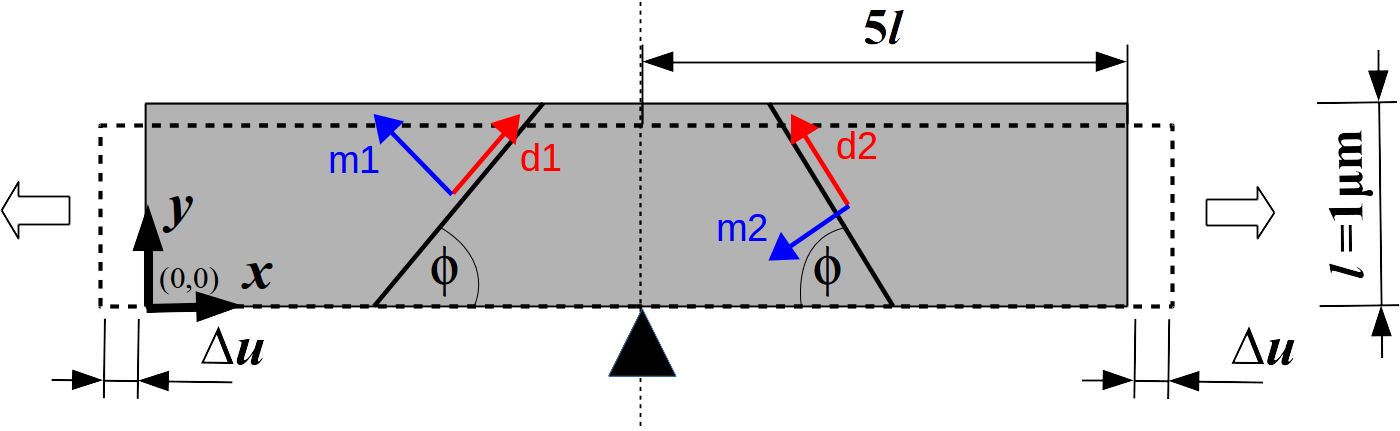
(a) Tensile test: Displacements are prescribed at left and right boundaries, top and bottom boundaries are free surfaces.

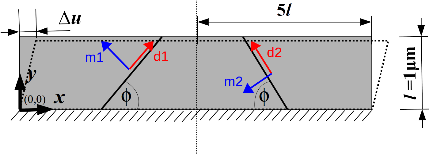
(b) Shear test: Displacements are prescribed at bottom and top boundaries, left and right boundaries are free surfaces.

Figure 2: Geometry and boundary conditions of the investigated model systems for the tensile test (Study 1 and Study 2) and the shear test (Study 3).

Geometry and slip system

We consider the configurations as shown in Fig. 2 for the investigation of the deformation behavior of a thin, single-crystalline Al film assuming plane strain. The film is represented by a 2-dimensional body $\mathcal{B}=(0,10l)\times(0,l)$ with $l=1$ µm. We consider one or two active slip systems ($N=1$ or 2) with 1-dimensional (crystallographic) slip planes determined by

$$\mathchoice{\mbox{\boldmath$\displaystyle\mathbf{d}$}}{\mbox{\boldmath$\textstyle\mathbf{d}$}}{\mbox{\boldmath$\scriptstyle\mathbf{d}$}}{\mbox{\boldmath$\scriptscriptstyle\mathbf{d}$}}^{1}=\cos\phi~{}\mathchoice{\mbox{\boldmath$\displaystyle\mathbf{e}$}}{\mbox{\boldmath$\textstyle\mathbf{e}$}}{\mbox{\boldmath$\scriptstyle\mathbf{e}$}}{\mbox{\boldmath$\scriptscriptstyle\mathbf{e}$}}_{1}+\sin\phi~{}\mathchoice{\mbox{\boldmath$\displaystyle\mathbf{e}$}}{\mbox{\boldmath$\textstyle\mathbf{e}$}}{\mbox{\boldmath$\scriptstyle\mathbf{e}$}}{\mbox{\boldmath$\scriptscriptstyle\mathbf{e}$}}_{2}\,, \mathchoice{\mbox{\boldmath$\displaystyle\mathbf{m}$}}{\mbox{\boldmath$\textstyle\mathbf{m}$}}{\mbox{\boldmath$\scriptstyle\mathbf{m}$}}{\mbox{\boldmath$\scriptscriptstyle\mathbf{m}$}}^{1}=-\sin\phi~{}\mathchoice{\mbox{\boldmath$\displaystyle\mathbf{e}$}}{\mbox{\boldmath$\textstyle\mathbf{e}$}}{\mbox{\boldmath$\scriptstyle\mathbf{e}$}}{\mbox{\boldmath$\scriptscriptstyle\mathbf{e}$}}_{1}+\cos\phi~{}\mathchoice{\mbox{\boldmath$\displaystyle\mathbf{e}$}}{\mbox{\boldmath$\textstyle\mathbf{e}$}}{\mbox{\boldmath$\scriptstyle\mathbf{e}$}}{\mbox{\boldmath$\scriptscriptstyle\mathbf{e}$}}_{2}\,,$$ (38a)

$$\mathchoice{\mbox{\boldmath$\displaystyle\mathbf{d}$}}{\mbox{\boldmath$\textstyle\mathbf{d}$}}{\mbox{\boldmath$\scriptstyle\mathbf{d}$}}{\mbox{\boldmath$\scriptscriptstyle\mathbf{d}$}}^{2}=-\cos\phi~{}\mathchoice{\mbox{\boldmath$\displaystyle\mathbf{e}$}}{\mbox{\boldmath$\textstyle\mathbf{e}$}}{\mbox{\boldmath$\scriptstyle\mathbf{e}$}}{\mbox{\boldmath$\scriptscriptstyle\mathbf{e}$}}_{1}+\sin\phi~{}\mathchoice{\mbox{\boldmath$\displaystyle\mathbf{e}$}}{\mbox{\boldmath$\textstyle\mathbf{e}$}}{\mbox{\boldmath$\scriptstyle\mathbf{e}$}}{\mbox{\boldmath$\scriptscriptstyle\mathbf{e}$}}_{2}\,, \mathchoice{\mbox{\boldmath$\displaystyle\mathbf{m}$}}{\mbox{\boldmath$\textstyle\mathbf{m}$}}{\mbox{\boldmath$\scriptstyle\mathbf{m}$}}{\mbox{\boldmath$\scriptscriptstyle\mathbf{m}$}}^{2}=-\sin\phi~{}\mathchoice{\mbox{\boldmath$\displaystyle\mathbf{e}$}}{\mbox{\boldmath$\textstyle\mathbf{e}$}}{\mbox{\boldmath$\scriptstyle\mathbf{e}$}}{\mbox{\boldmath$\scriptscriptstyle\mathbf{e}$}}_{1}-\cos\phi~{}\mathchoice{\mbox{\boldmath$\displaystyle\mathbf{e}$}}{\mbox{\boldmath$\textstyle\mathbf{e}$}}{\mbox{\boldmath$\scriptstyle\mathbf{e}$}}{\mbox{\boldmath$\scriptscriptstyle\mathbf{e}$}}_{2}$$ (38b)

with the angle $\phi=\pi/3$ between slip planes and the film surfaces. The distance between crystallographic slip planes is set to ${\vartriangle}s=0.05,0.1,0.2$ µm, respectively. For the thickness of the crystallographic layer $\mathcal{B}_{s,g}$ we choose $h=0.5{\vartriangle}s$. In Case 2, we set ${\vartriangle}\overline{s}=0.2,0.4$ µm. As material we use aluminum with a Young’s modulus of $E=7\cdot 10^{10}$ Pa, Poisson ratio $\nu=0.3$, Burgers vector size $b=2.56\cdot 10^{-10}$ m and drag coefficient $B=2.0\cdot 10^{-4}$ Pa$\cdot$s.

Numerical aspects

We use two different finite element meshes: the mesh for the elastic problem consists of triangular linear finite elements with altogether $\approx 223\,000$ degrees of freedom (dofs), the hdCDD mesh consists of linear Fourier elements with, e.g. $\approx 262\,000$ dofs for Case 1 with ${\vartriangle}s=100$ nm and $h=50$ nm. For the time integration we used a step size of ${\vartriangle}t=10^{-3}$µs with $M=10$ ’micro-time steps’ per macroscopic displacement increment, resulting in $6\cdot 10^{3}$ micro-time steps for reaching the total strain of $\varepsilon^{\text{tot}}=1.2\%$. For the shear test the same step size is used with a total number of $5\cdot 10^{3}$ micro-time steps for obtaining the total strain of $\varepsilon^{\text{tot}}=2.5\%$. During each of the micro-time steps the stresses from the elastic BVP are kept constant and only the dislocation microstructure with the respective short-range interaction stresses evolves.

Boundary conditions

For the two different systems we introduce different boundary conditions for the elasticity problem:

• For the symmetric tensile test we consider prescribed boundary displacements along the left and right boundary face (at $x_{1}=0$ and $x_{1}=10l$, respectively). We increase the displacements with a constant rate $\dot{u}_{1,{\rm right}}=-\dot{u}_{1,{\rm left}}=1.0$ m/s for $t\in[0,0.06]$ µs. In order to avoid vertical translations we additionally fix the displacements at the point $(5l,0)^{\top}$.

• For the shear test we consider prescribed boundary displacements along the upper surface at $x_{2}=l$ and fixed displacements at the lower surface at $x_{2}=0$. The upper prescribed displacements are increased with a constant rate $\dot{u}_{1,\rm{up}}=1.0$ m/s for $t\in[0,0.05]$ µs.

For both systems, also the boundary conditions for the dislocation problem w.r.t. dislocation fluxes have to be considered. In physical terms surfaces can either be open (dislocations can leave the film) or impenetrable (dislocations can not leave the film). Open boundaries can simply be modeled by extrapolating the hdCDD field values. For impenetrable surfaces we require (i) that the flux of dislocation density normal to the surface vanishes and that (ii) dislocations directly at the surface must be straight and thus must have zero curvature. Numerically, we model the impenetrable flux boundary condition by introducing a numerical inflow defined as the negative outflow of density and curvature densities on the considered boundary.

Initial values

We construct consistent initial values which guarantee that, e.g., the solenoidality of ${\mathchoice{\mbox{\boldmath$\displaystyle\mathbf{\alpha}$}}{\mbox{\boldmath$\textstyle\mathbf{\alpha}$}}{\mbox{\boldmath$\scriptstyle\mathbf{\alpha}$}}{\mbox{\boldmath$\scriptscriptstyle\mathbf{\alpha}$}}}^{\text{I\!I}}$ (i.e. $\operatorname*{div}{\mathchoice{\mbox{\boldmath$\displaystyle\mathbf{\alpha}$}}{\mbox{\boldmath$\textstyle\mathbf{\alpha}$}}{\mbox{\boldmath$\scriptstyle\mathbf{\alpha}$}}{\mbox{\boldmath$\scriptscriptstyle\mathbf{\alpha}$}}}^{\text{I\!I}}=0$) is not violated and that the GND density vector comes out as a gradient of the plastic slip. This is done by superposition of $N_{\rm d}$ randomly distributed discrete dislocation loops in a 2D slip plane followed by an appropriate ’smearing-out’ procedure as described in detail in the appendix. One-dimensional slip plane data are then obtained by integrating the CDD field values over the second, homogeneous direction (see Fig. 3). Depending on the used averaging, i.e. Case 1 or 2, we finally have to consider the distance of the representative slip planes.

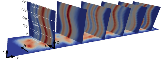
Figure 3: Visualization of the initial dislocation density in the higher-dimensional configuration space for a system with 25 representative slip planes, each of them containing 28 ’smeared-out’ randomly positioned loops. In vertical direction the variable $\varphi\in[0,2\pi]$ is displayed for some of the 25 slip planes; the dashed white lines indicate the line orientation for screw and edge segments (compare Burgers vector direction in the spatial plane). Each of the wavy distributions corresponds to (a) dislocation loop(s). On the bottom plane the spatial projection of the total density $\rho^{\text{tot}}$ is shown as spatial average as seen in ’Case 2’.

4.1 Study 1: The influence of boundary conditions (Case 1)

For this investigation we use 80 representative slip planes and the shear strain extension of Case 1, starting in each SP with 5 dislocation loops of radius $r$ between 100 nm and 200 nm at random positions. The height of the quasi-discrete numerical SPs has a relatively small value of $h=50$ nm below which no appreciable difference in the system response could be observed (also see Study 2). For averaging purposes we assume an out-of-plane length of $L_{z}=l/\sin(\phi)=1.15$ µm resulting in an average dislocation density $\langle\rho\rangle=3.1\times 10^{13}/{\rm m}^{2}$. For the analysis of the influence of boundary conditions we study two configurations: in the first configuration we choose open boundaries (abbreviated as ’open BCs’), i.e. dislocations can leave the volume, and the second imposes impenetrable boundaries (abbreviated as ’imp. BCs’), i.e. dislocations can not leave the volume through the surface $\partial B$. The simulation is driven by a prescribed constant strain rate $\dot{\varepsilon}=0.2$ µs^-1 until the maximum total strain $\varepsilon^{\rm tot}=1.2\%$ is reached.

                

Figure 4: Initial distribution and time evolution of total density $\rho^{\text{tot}}$, Case 1, with open and impenetrable boundary conditions for the dislocation density.

In Fig. 4 the evolution of the total density $\rho^{\rm tot}$ at three distinct time steps in the $x-y$-plane is illustrated.

We observe that the configuration with open boundaries approaches a constant total density distribution along the slip planes while the system with impenetrable boundaries forms pile-ups of dislocations at the boundary with constant density values in between. To analyze this behavior we investigate the dislocation microstructure in the higher-dimensional configuration space for a slip plane in the center of the film in more detail (Fig. 5).

                                

Figure 5: Time evolution of hdCDD density $\rho(\xi,\varphi)$, curvature density $q(\xi,\varphi)$ and curvature $k(\xi,\varphi)=q(\xi,\varphi)/\rho(\xi,\varphi)$ for open (left block) and impenetrable boundaries (right block) for a slip plane with random initial values taken from the center region of Fig. 4. On the vertical axis is the line orientation $\varphi\in[0,2\pi]$, on the horizontal axis is the local $\xi$ coordinate, the small text label indicates the maximum field value.

The higher-dimensional fields show that for both dislocation boundary conditions after an initial ’incubation’ time the center region of the slip plane approaches a state which is characterized by only screw dislocations of positive and negative orientation: $\rho(x,\varphi)$ is approximately non-zero only for the orientations $\varphi=\pi/2$ and $\varphi=3\pi/2$. The reason for this is that dislocation loops expanded and segments with edge orientation either left the film through the surface or pile up against the surface. In any case, only screw segments are left behind which in this 2D model thread the film into the out-of-plane direction. Investigating the curvature $k=\rho/q$ we also see that the screw segments are nearly straight (i.e. $k\approx 0$); only for the impenetrable boundaries we find a non-zero curvature shortly before the surface: here, dislocations need to bend strongly in order to adjust from the threading screw dislocation orientation to the geometry of the films’ surface.

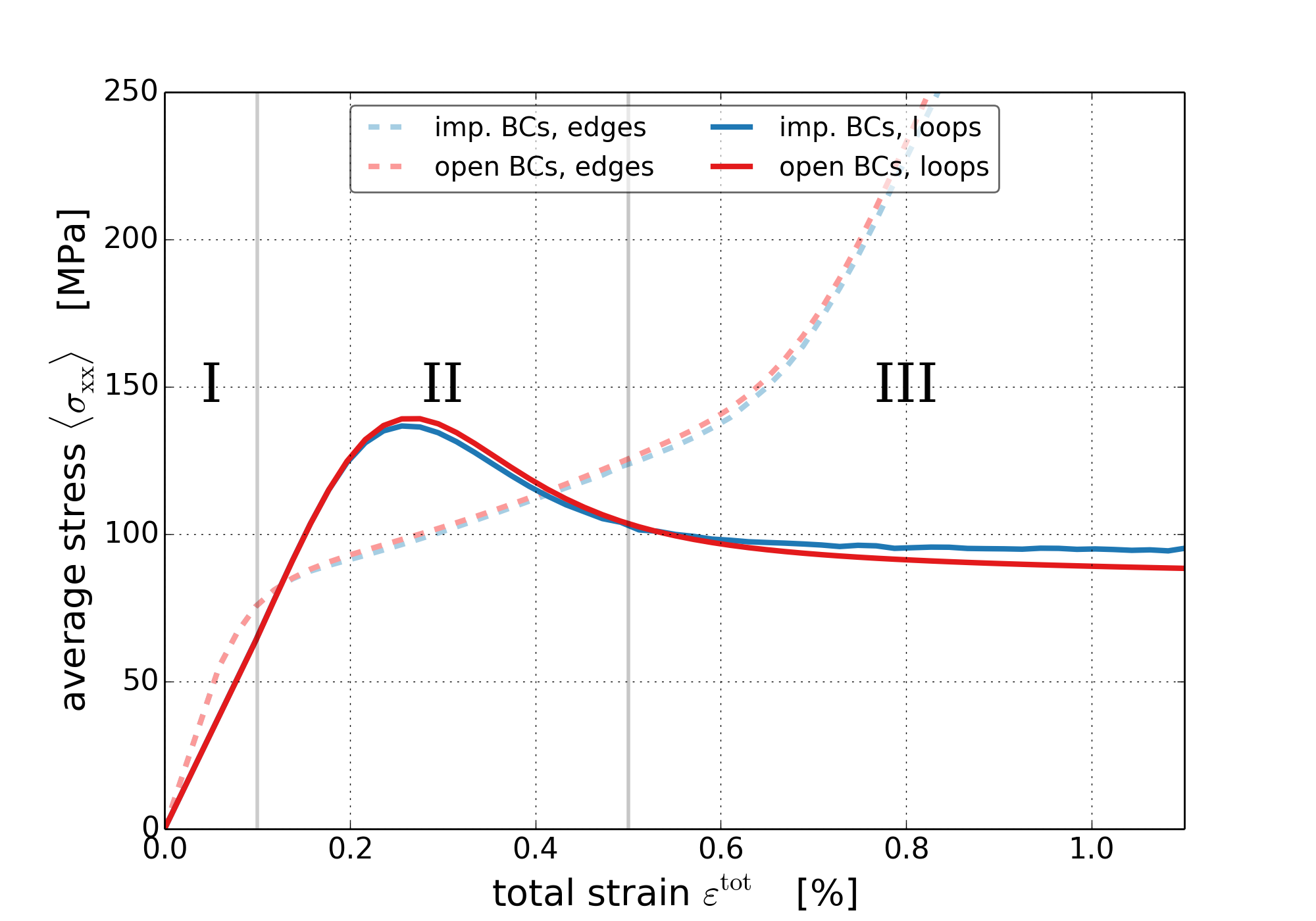
(a) average stress vs. total strain

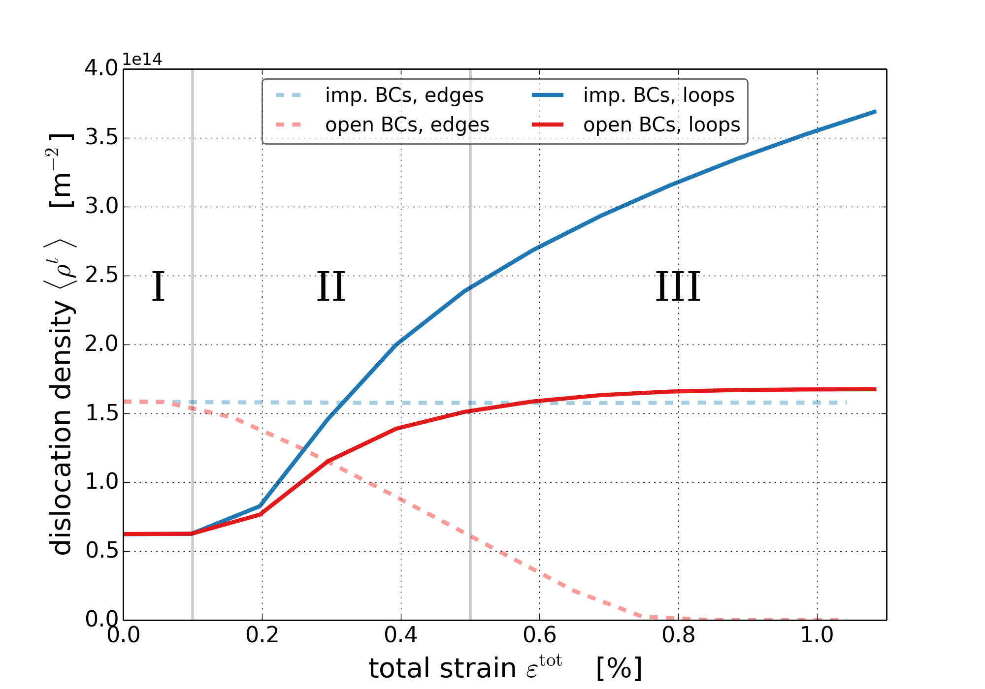
(b) average total density vs. total strain

Figure 6: Macroscopic quantities (Case 1) for two different boundary conditions (open and impenetrable) and two different initial configurations (consisting of either only loops or only straight edge dislocations). The three different time snapshots in Fig. 5 correspond to the different regimes I, II, and III, respectively.

This also suggests that the amount of dislocations inside the film for the impenetrable system will be significantly higher: to begin with, dislocations are not ’lost’ by out-flux through the surfaces, and an additionally increased line length production will take place due to the high dislocation curvature near the surfaces. Plotting the average density evolution in Fig. 6 (b) shows that in the elastic regime I the dislocation density is constant, i.e. the resolved shear stress is not large enough to overcome the yield stress. This is followed in regime II by a transition of ’free loop expansion’ which results in a high dislocation multiplication rate. Towards regime III, edge components are then lost through open surfaces, while for impenetrable BCs edge dislocations are deposited at the surfaces. The open system contains at final strain a density which is smaller roughly by a factor of 3, and additionally the average density even reaches a stationary state (threading screw segments are straight and thus only translate). For the system with impenetrable surfaces the average density increases approximately linearly (caused by the constant line length increase of deposited edges).

What are the consequences for the macroscopic stress-strain response? A higher dislocation density, on the one hand, obviously comes with a stronger influence of the Taylor equation for the yield stress. On the other hand, a higher plastic activity, where the density comes in through the Orowan relation, causes plastic softening through the solution of the elastic eigenstrain BVP. The competition of these two effects can be observed in the macroscopic stress-strain curve in Fig. 6 (a) where at larger strains the obtained stress level for the system with open boundaries is only slightly lower. Interesting to note is also the initial ’hump’ right after the elastic regime I when softening sets in. This is caused by the fact that at an early stage dislocation loops are still comparatively small and thus contribute with a high line tension effect which effectively reduces the resolved shear stress. Once loops have expanded, this contribution is reduced and the softening behavior is sustained. A very similar behavior is also observed in DDD simulations (Weygand and Gumbsch, 2005).

Finally, we compare the evolution of the initial dislocation loop distribution to a distribution of positive and negative edge dislocations (dashed lines in Fig. 6), which would be the equivalent of a ’Groma-type model’. Therefore, we choose the number of edge dislocations such that the initial density is similar to the saturation density of loops with open BCs. We observe that after the onset of plastic yield edge dislocations flow towards the surfaces (regime II). They either get lost through the surfaces (open BCs) or pile up against the surface (imp. BCs) in which case the density simply stays constant because the number of edge dislocations in preserved. This microstructure results in a dramatically different stress-strain response as compared to the system with curved dislocations: because we have neither an increase in density nor a line tension one can only observe a linear hardening (regime II) which – regardless the boundary condition – is followed by a nearly elastic regime III where the stresses are considerably different from those reached for the system with dislocation loops. The loss of dislocations through surfaces (and ultimately the ’dislocation starvation’) has been experimentally observed in nano/micro pillar compression tests (Shan et al., 2008; Jerusalem et al., 2012) as well. This starvation effect also gave rise to a second elastic regime as observed in our edge dislocation system. In a 3D geometry we also would find this for a distribution of dislocation loops and open BCs.

4.2 Study 2: Spatial coarsening from Case 1 to Case 2

In Case 1 we considered slip planes as quasi-discrete objects mimicking the situation in DDD simulations. This not only requires a very high spatial resolution for the finite element scheme, but it is also somewhat unsatisfying from a conceptual point of view to have two different resolutions (within the slip plane and perpendicular to it). If this can be avoided by use of Case 2 and whether it is admissible will be studied subsequently: for a given initial distribution of dislocations loops we compare the asymptotic system response for $h\rightarrow 0$ in Case 1 and then compare with results obtained for different values of ${\vartriangle}\overline{s}$ in Case 2.

   

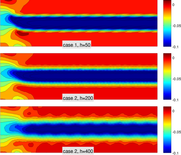
(a) Distribution of the stress component $\sigma_{xx}$ on the left half part $(0,5l)\times(0,l)$.

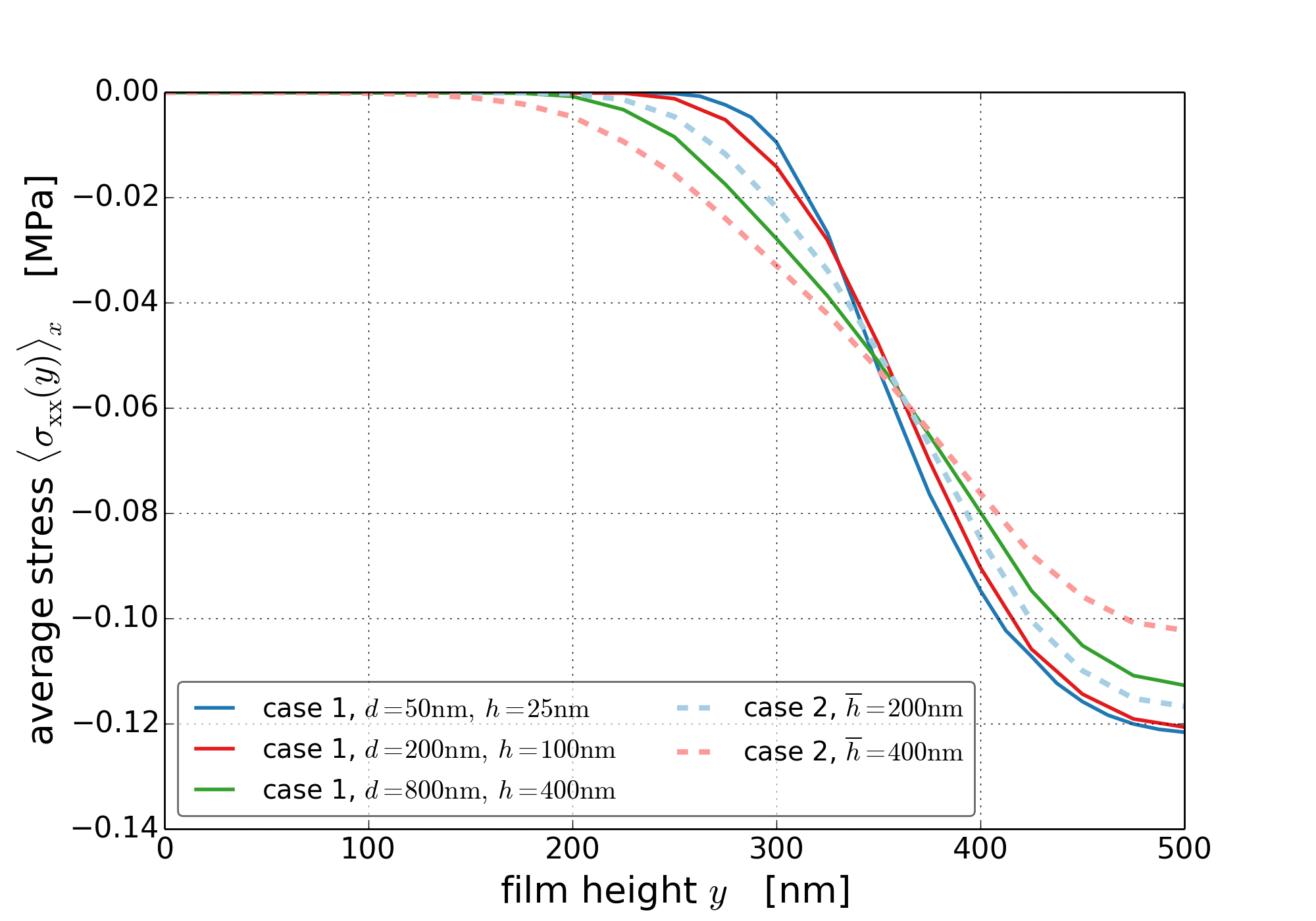
(b) Averaged stress $\langle\sigma_{xx}\rangle=\frac{1}{L_{x}}\int_{0}^{L_{y}}\sigma_{xx}\,{\rm d}x$ at $\varepsilon^{\rm tot}=0$.

Figure 7: Comparison of Case 1 and Case 2 for different numerical SP heights at $t=0$ for a homogeneous distribution of loops of the same radius. (a) shows the spatial stress distribution, (b) shows averaged stress profiles across the height. Since the configuration is symmetric, only half of the profile is shown.

All system and geometry properties are the same as in the previous Study 1, but this time we only compute stresses for a given dislocation configuration. To make the configurations easier to compare we simply choose a homogeneous distribution of loops. Fig. 7 (a) shows the resulting stresses for the quasi-discrete Case 1 for a SP height of $h=50$ nm and two different discretizations for Case 2. If we average these stress distributions we obtain stress profiles as shown in Fig. 7 (b). It shows that for values of $h=100$ nm and below the stresses do not change appreciably anymore. Running the same simulations for Case 2 where the plastic strain is coarse grained in between the numerical SPs and comparing with the results for Case 1 allows for the conclusion that for this system a ${\vartriangle}\overline{s}=200$ nm is sufficient; also the stress-strain behavior (not shown) does not show any significant difference. The considered situation of a homogeneous loop distribution is of course artificial. In fact, differences during time evolution in particular between the very coarse Case 2 and the fine Case 1 become larger if we start with the random initial values and as the plastic slip becomes more heterogeneous (early in regime II). Nonetheless, even there, our chosen approximation of Case 2 with ${\vartriangle}\overline{s}=200$ nm is sufficient.

The advantage of the interpolation approach used in Case 2 becomes obvious when we take a look at the degrees of freedoms and the computational time used for the simulations from Study 1 shown in Tab. 1: using Case 2 with ${\vartriangle}\overline{s}=200$ nm instead of Case 1 even with ${\vartriangle}s=100$ nm, $h=50$ nm gives already a speedup factor of nearly 2, while at the same time no appreciable differences in the results - also for the time dependent simulations - could be observed.

configuration	dofs (FEM + DG)	comp. time in h on 8 procs.
Case 1, ${\vartriangle}s=\phantom{0}50$ nm, $h=\phantom{0}25$ nm	214 962 + 1 049 600	7:39:33
Case 1, ${\vartriangle}s=100$ nm, $h=\phantom{0}50$ nm	54 682 + 0262 400	1:49:01
Case 1, ${\vartriangle}s=200$ nm, $h=100$ nm	54 682 + 0131 200	1:00:35
Case 2, ${\vartriangle}\overline{s}=200$ nm	54 682 + 0131 200	1:00:44
Case 2, ${\vartriangle}\overline{s}=400$ nm	54 682 + 0065 600	0:46:04

Table 1: Comparison of computational time and degrees of freedom for Case 1 and Case 2.

4.3 Study 3: A double slip configuration with Case 2

We now investigate the macroscopic elasto-plastic response together with the microstructural evolution in a configuration with the two slip systems (38). We use fully averaged dislocation distributions (Case 2 with ${\vartriangle}\overline{s}=200$ nm), and the interaction of the dislocation densities in the two systems is described by the yield stress

$$\tau^{\text{y}}_{s,g}=a\mu b_{s}\sqrt{\rho^{\text{tot}}_{1}+\rho^{\text{tot}}_{2}}\,,$$ (39)

where $\rho^{\text{tot}}_{s}$ is reconstructed in $\mathcal{B}$ from $\rho^{\text{tot}}_{s,g}$ by averaging and interpolation using the construction (15). This particular form of the yield stress represents that dislocations on the one slip system act as forest for the family of dislocations on the other slip system and vice versa (see e.g. Kubin et al., 2008). The line tension is obtained in full analogy to Study 1 for each slip system separately. Subsequently, we compare a single slip and double slip scenario with the following initial distribution of the dislocation density: in both cases we have altogether 800 dislocation loops in an averaging volume for which we again assume an out-of-plane averaging length of $L_{z}=1.15$ µm. The loops’ radii are taken from a uniform random distribution in the range of $[100,200]$ nm. We either distribute them across the two slip systems or only across a single slip system such that the average dislocation density in the full body is always the same. In this study we only consider open boundaries since we focus here on the investigation of the hardening/softening effects introduced by the interaction of the slip systems and the concomitant change in dislocation microstructure. The results are illustrated in Fig. 8 –10.

Initially ($\varepsilon^{\rm tot}\leq 0.2\%$) both systems respond nearly perfectly elastic because the resolved shear stress is in almost all regions smaller than the yield stress. This can be seen in the linear increase in Fig. 9a which is a consequence of the (nearly) zero velocity in Fig. 8 (c) and (f).

Eventually ($0.2\%<\varepsilon^{\rm tot}<0.5\%$), starting from the outer regions of the density distribution where $\rho^{\rm tot}$ is smaller, the yield stress will be overcome. This results in a non-zero dislocation velocity mainly in the surface-near regions (Fig. 8 (c) and (f) and further plots shown in appendix B). Already shortly after $\varepsilon^{\rm tot}=0.2\%$ it becomes visible that the single slip and double slip systems behave very differently. The reason for this lies in the crystallography of the model systems: the Burgers vectors of the symmetrically inclined slip systems are such that under the prescribed shear deformation the diagonal components in the plastic strain tensors will cancel out. This results in a higher resolved shear stress since the plastic softening contribution is smaller. At the same time, however, the resulting velocity is higher, giving rise to more dislocation activity which can be observed in the plastic strain profile (compare Fig. 8 (b) and (e)). For the single slip situation these relations are just the other way around: the plastic slip reduces the resolved shear stress and thus the dislocation velocity. The reduced plastic activity also shows in the evolution of the dislocation density and plastic slip which happens at a lower rate than for the double slip system, cf. Fig. 9b.

profiles for the single slip configuration

profiles for the double slip configuration

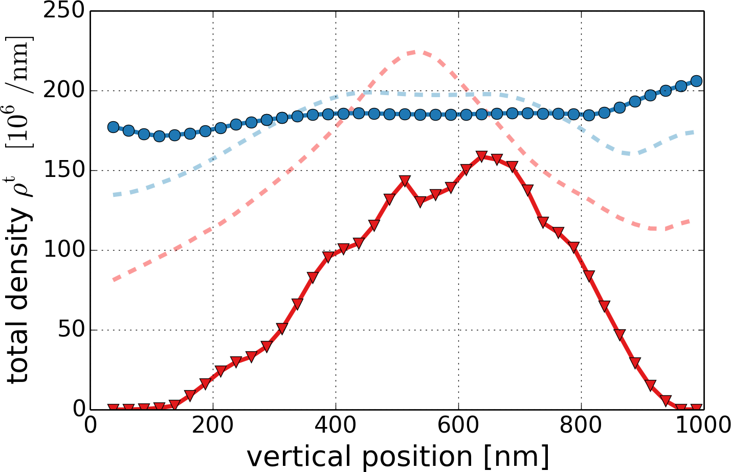
(a) total density

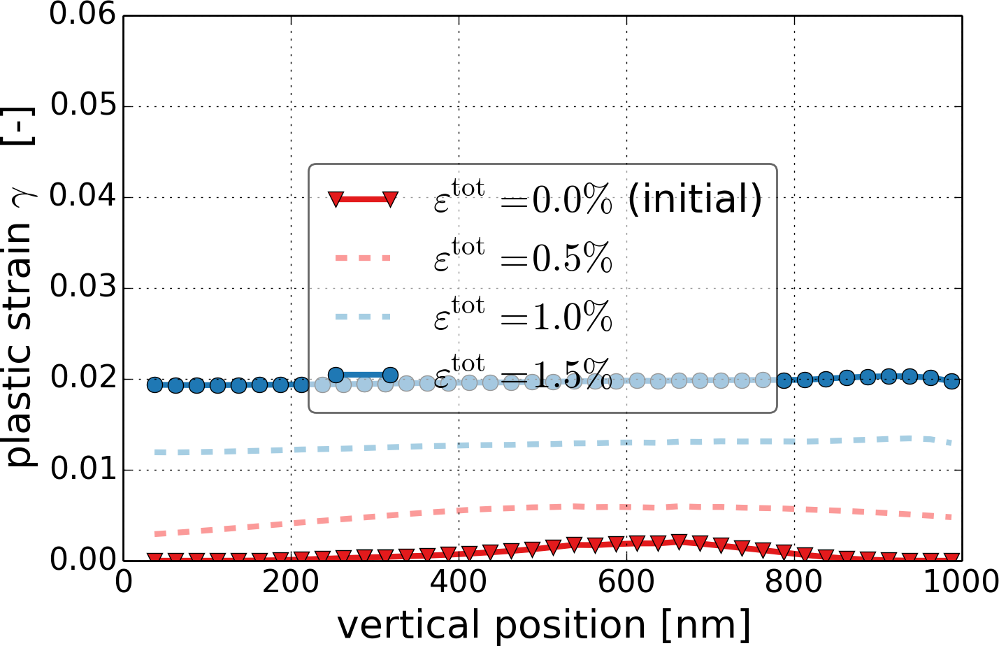
(b) plastic slip

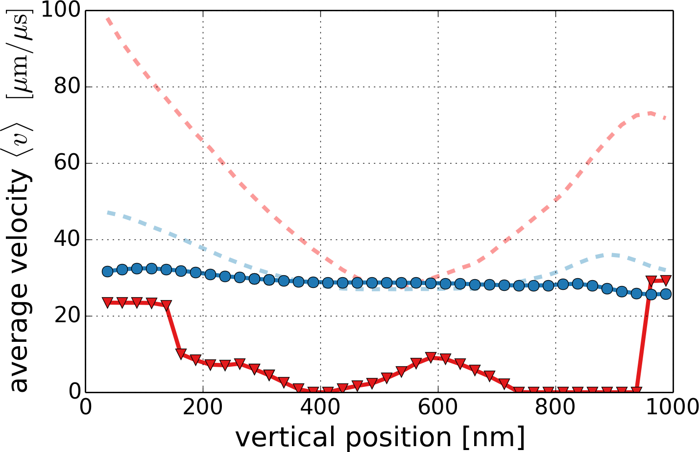
(c) velocity

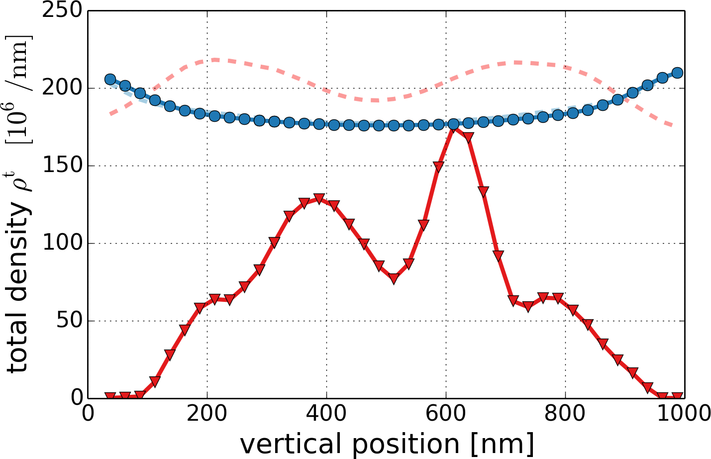
(d) total density

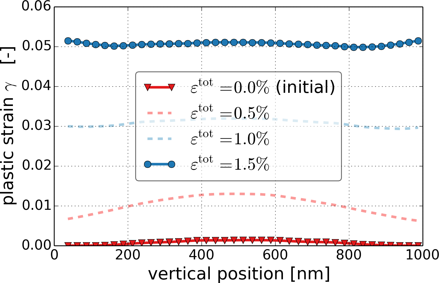
(e) plastic slip

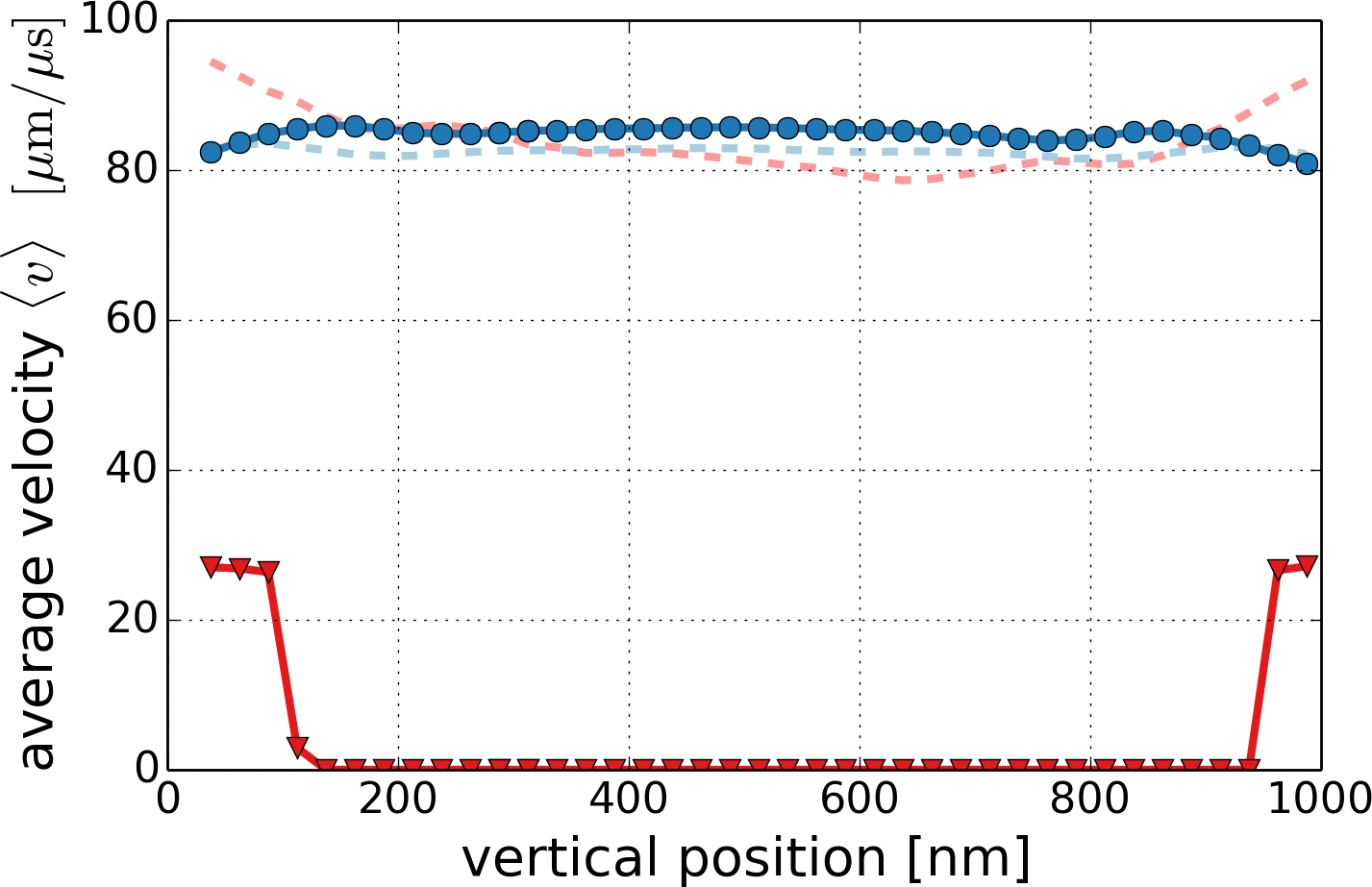
(f) velocity

Figure 8: Profiles of CDD field variables along a central slip plane for the single slip (a-c) and double slip configuration (d-f) for 4 different time steps. Double slip density values and plastic slip (d-f) were multiplied by a factor of 2 to make them comparable with the single slip situation.

We will now take a closer look at details of the stress-strain curve (Fig. 9a). What causes the ’humps’ and different maxima for single/double slip following the elastic regime at $\varepsilon^{\rm tot}\approx 0.5\%$? Fig. 10 shows the higher-dimensional density, curvature density and curvature fields. There it can be seen, that for the single slip system the lower velocity broadens the density distribution but does not allow for a more significant expansion of loops and thus retards the density production. As a consequence of the reduced loop expansion, the loops’ curvature is also much higher for the single slip system, giving rise to a more pronounced influence of the line tension (cf. plots in Appendix B); as a consequence of the retarded density production the yield stress is effectively lower. The latter shows in Fig. 9a in the lower maximum of the hump as compared to the double slip situation; the former shows in the steeper inclination following the hump. While loops expand the influence of the line tension becomes smaller and tends to zero with edge segments leaving the film and screw dislocations becoming straight lines. The influence of the yield stress approaches a constant value once the density from the nearly straight edge dislocations saturates. Therefore, towards larger total strains ($>2\%$) the only difference between the single and double slip system stems from the plastic strain, while microscopic, short-range stresses had a stronger influence on early details of the stress-strain response.

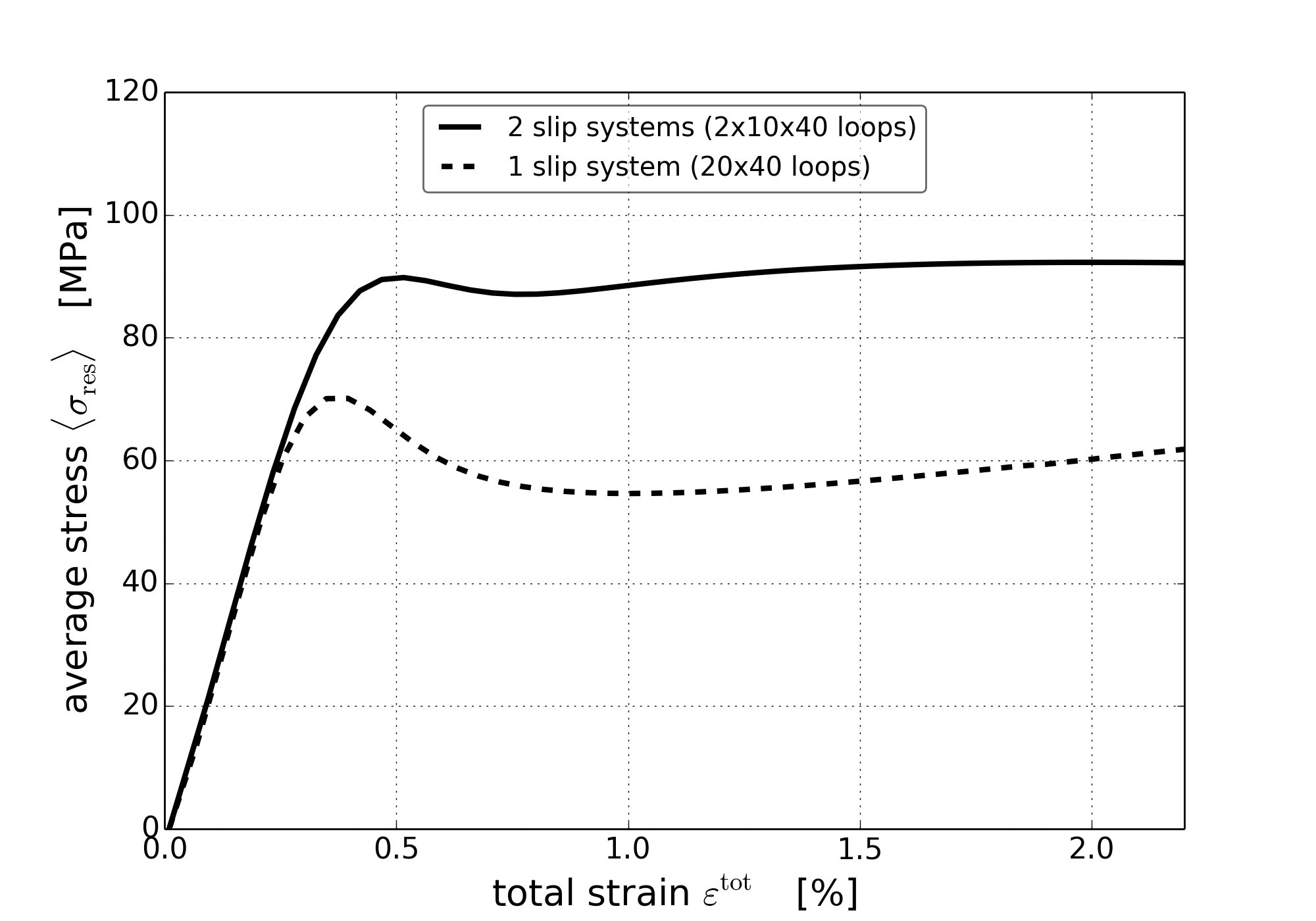
(a) average resolved shear stress vs. total strain

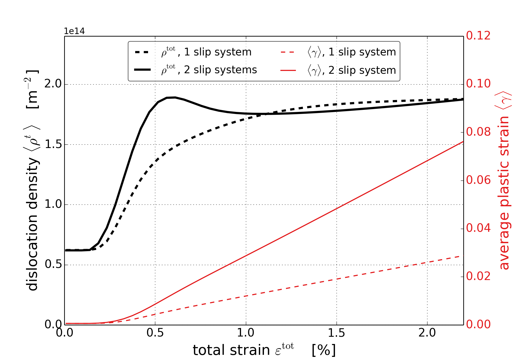
(b) average total density vs. total strain

Figure 9: Stress-strain plot and evolution of total density and plastic slip for the single slip and double slip configuration.

                                

Figure 10: Time evolution of hdCDD density $\rho(\xi,\varphi)$, curvature density $q(\xi,\varphi)$ and curvature $k(\xi,\varphi)=q(\xi,\varphi)/\rho(\xi,\varphi)$ for open boundaries, left: in single slip configuration (compare Study 1, Fig. 5) and right: in double slip configuration with random initial values taken from the center region of Fig. 11. On the vertical axis is the line orientation $\varphi\in[0,2\pi]$, on the horizontal axis is the local $\xi$ coordinate, the small text label indicate the maximum field value (comparison with Fig. 5 of Study 1).

5 Summary and Conclusion

Modeling and prediction of crystal-plasticity on the micro-meter scale requires a faithful representation of the underlying physical mechanisms. We introduced the higher-dimensional CDD theory as a mathematical description of the kinematic behavior of statistically averaged ensembles of dislocations. A special emphasis was put on a consistent geometric description of the CDD field equations for the general case of arbitrarily oriented slip systems. In particular the transfer of information from two-dimensional crystallographic slip planes to the three-dimensional continuous body was concisely formulated. Furthermore, a conservative discontinuous Galerkin scheme suitable for the dislocation problem was derived. These model formulations were then applied to simulate different plain-strain slip geometries under tensile and shear loading conditions together with different physical boundary conditions. We analyzed in detail how systems of dislocation evolve while they interact with each other due to short-range and long-range stress components. In doing so we could directly link the dislocation microstructure – represented by the higher-dimensional density and curvature density – to the macroscopic behavior (e.g. stress-strain response or average density). By comparing to systems of straight edge dislocations we observed that there the line curvature has a strong influence on the initial hardening behavior which is then complemented by a sustained influence of mobile screw dislocations: the quantitative and qualitative change in the stress-strain curve could be well explained by hdCDD. Furthermore, we showed how physical boundary conditions influence the orientation distribution of dislocations and again, how this impacts the system response. Finally, we studied a double slip configuration where we could attribute the distinctly different hardening behavior for single/double slip to microstructural aspects.

The hdCDD model contains microstructural information which otherwise is only available in DDD simulations. These microstructural details have a strong influence on the system response, which is why a comparison with other models is difficult: no other standard continuum plasticity model is able to represent e.g. the conversion of SSDs into GNDs and the dislocation line length production accompanied by expansion of dislocation loops. For this, direct comparisons with DDD simulation will be extremely interesting and helpful to further benchmark our model. The necessary extraction of information from DDD simulations and conversion into continuous fields, however, is a non trivial task which needs to be undertaken with care in future work. More realistic CDD systems will additionally require to incorporate further dislocation interactions and reactions as well as mechanisms for dislocation sources or annihilation which are not a priori included in the CDD theory (see e.g. Sandfeld and Hochrainer (2011) and Zhu et al. (2014) for steps into this direction). DDD simulations will be very useful there as well. With this we hope to go beyond what up to date is possible with DDD and apply CDD to realistic three-dimensional systems with large numbers of interacting dislocations and plastic strain.

Appendix A: Computation of consistent initial values

Special care has to be taken with creating initial values for CDD simulations. ’Consistent initial values’ are those which represent averaged systems of dislocations such that the solenoidality of ${\mathchoice{\mbox{\boldmath$\displaystyle\mathbf{\alpha}$}}{\mbox{\boldmath$\textstyle\mathbf{\alpha}$}}{\mbox{\boldmath$\scriptstyle\mathbf{\alpha}$}}{\mbox{\boldmath$\scriptscriptstyle\mathbf{\alpha}$}}}^{\text{I\!I}}$ is not violated, i.e. $\operatorname*{div}{\mathchoice{\mbox{\boldmath$\displaystyle\mathbf{\alpha}$}}{\mbox{\boldmath$\textstyle\mathbf{\alpha}$}}{\mbox{\boldmath$\scriptstyle\mathbf{\alpha}$}}{\mbox{\boldmath$\scriptscriptstyle\mathbf{\alpha}$}}}^{\text{I\!I}}=0$. An additional constraint is the compatibility between a resulting GND density and the plastic shear, $\mathchoice{\mbox{\boldmath$\displaystyle\mathbf{\kappa}$}}{\mbox{\boldmath$\textstyle\mathbf{\kappa}$}}{\mbox{\boldmath$\scriptstyle\mathbf{\kappa}$}}{\mbox{\boldmath$\scriptscriptstyle\mathbf{\kappa}$}}^{\perp}=-\frac{1}{b}\nabla\gamma_{s}$. One way of guaranteeing these conditions is to create initial values in a 2-dimensional slip plane by superposition of objects which a priori fulfill these conditions. E.g. one may choose a closed dislocation loop of radius $R$ with center point $\mathbf{r}_{0}$; a point $\mathbf{r}$ in $\Gamma_{s,g}$ then has the distance $d=|R(-\sin\varphi,\cos\varphi)+\mathbf{r}_{0}-\mathbf{r}|$ from the loops’ line and the density and the curvature can be obtained by ’smearing-out’ the line such that the total line length $2\pi R$ is preserved, i.e.,

$$\rho(\mathbf{r},\varphi)=\begin{cases}\frac{R\exp(-1/(1-(d/d_{0})^{2}))}{2\pi\int_{0}^{d_{0}}t\exp(-1/(1-(t/d_{0})^{2}))\,\mathrm{d}t}&\quad{\rm if}\quad d<d_{0}\,,\\ 0&\quad\text{else,}\end{cases}$$

where the parameter $d_{0}$ governs the width of the compact density distribution around the line. Note, that this results in an area density i.e. $\rho$ has the unit of line length per area. The curvature density can be obtained as $\displaystyle q(\mathbf{r},\varphi)=\frac{\rho(\mathbf{r},\varphi)}{R}$. The corresponding plastic slip generated by the expanded loop is given by $\displaystyle\gamma(\mathbf{r})=b\int_{|\mathbf{r}-\mathbf{r}_{0}|}^{R+d_{0}}\int_{0}^{2\pi}\rho(\eta,0,\varphi)\,{\rm d}\varphi\,{\rm d}\eta$. We superimpose $N_{d}$ such dislocation loops with randomly chosen centers of the loops with a uniform distribution and such that the compact function for the CDD fields fits completely into the slip plane. Additionally, the loops’ radii are chosen from a uniform random distribution. The 1D-slip planes represent a homogeneous distribution into the second direction, so that we integrate the CDD fields along the width for $\rho_{s,g}(\xi),q_{s,g}(\xi)$ and $\gamma_{s,g}(\xi)$, see Fig. 3 for an visualization.

Appendix B: Evolution of CDD field quantities for Study 3

The following figures show the evolution of total density for the single and double slip system (Fig. 11). The largest difference in these two situations is that due to the different stress state in double slip the dislocation activity is much more pronounced. In Fig. 12 also the profiles for all relevant CDD field quantities and stress components are shown. One of the key feature of hdCDD is that the distinction into GNDs and SSDs is obtained naturally from the higher-dimensional configuration space. This can be also observed in the evolution of the integrated quantities $\rho^{\rm tot}$ and $\kappa^{\rm edge}$ in Fig. 12 (a)+(b) and (g)+(h). Therein, the difference $\rho^{\rm tot}-|\kappa^{\rm edge}|$ would yield the SSD density of edges.

                      

Figure 11: Initial distribution and time evolution of total density $\rho_{s,g}^{\text{tot}}$ for Case 2, Study 3, for system with $s=1$ and $s=1,2$ at $t=0.01$ µs and $t=0.02$ µs with open boundary conditions for the dislocation density.

profiles for the single slip configuration

(a) total density

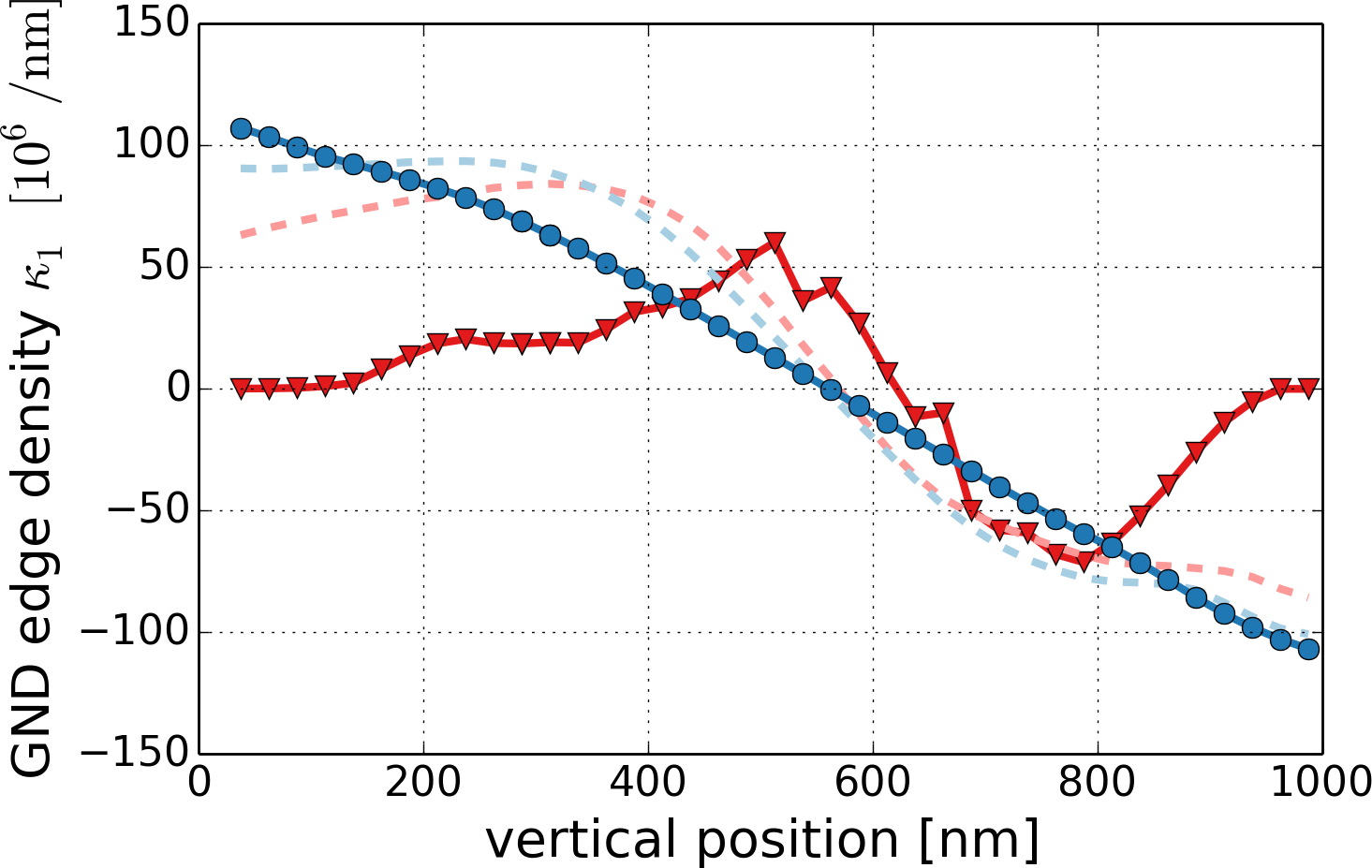
(b) GND density (edges)

(c) plastic slip

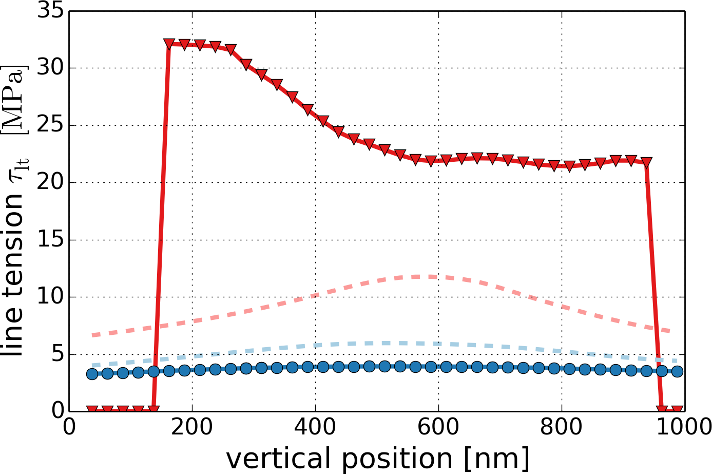
(d) line tension

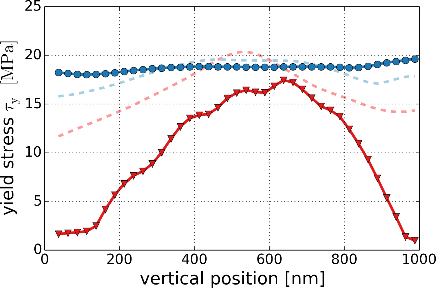
(e) yield stress

(f) velocity

(g) total density

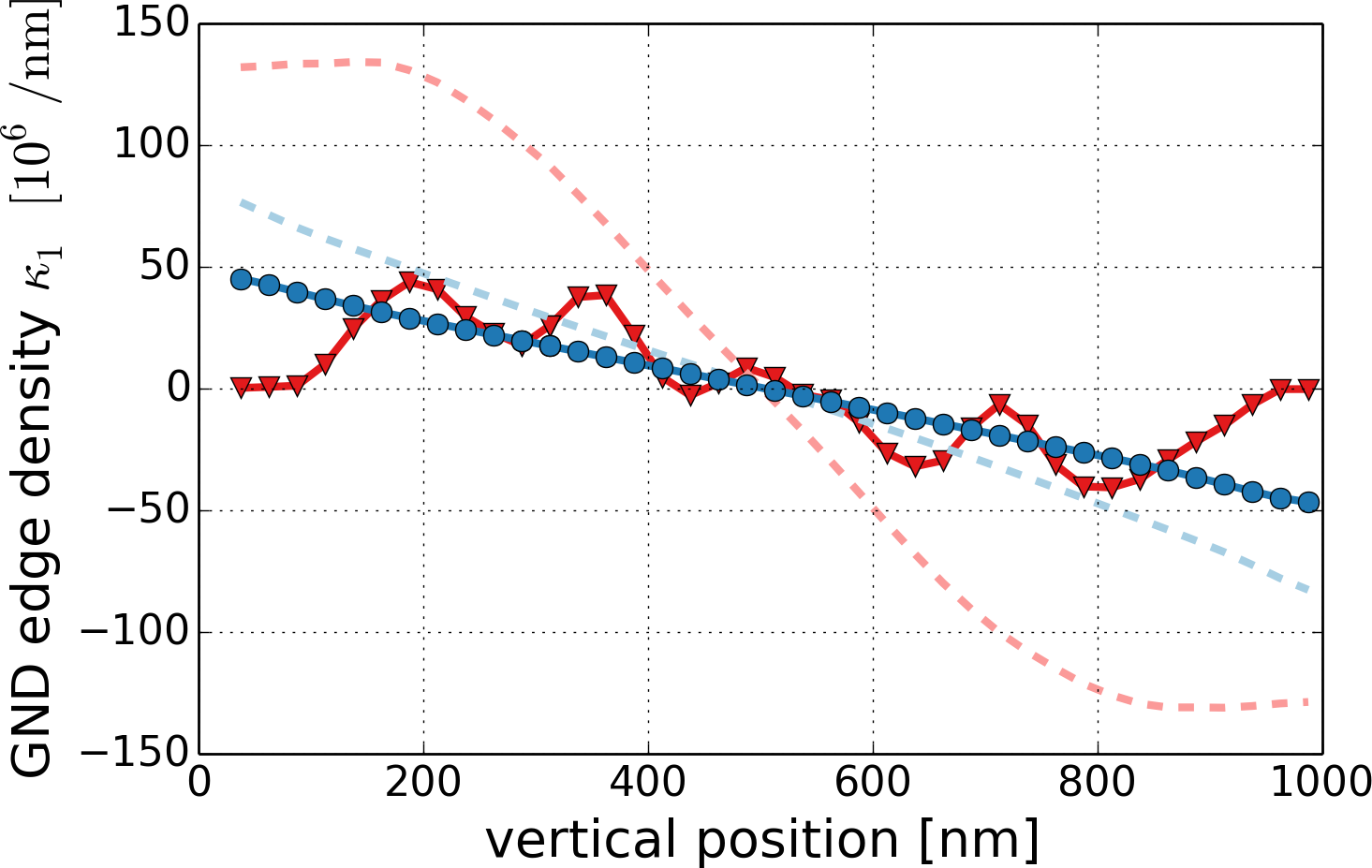
(h) GND density (edges)

(i) plastic slip

profiles for the double slip configuration

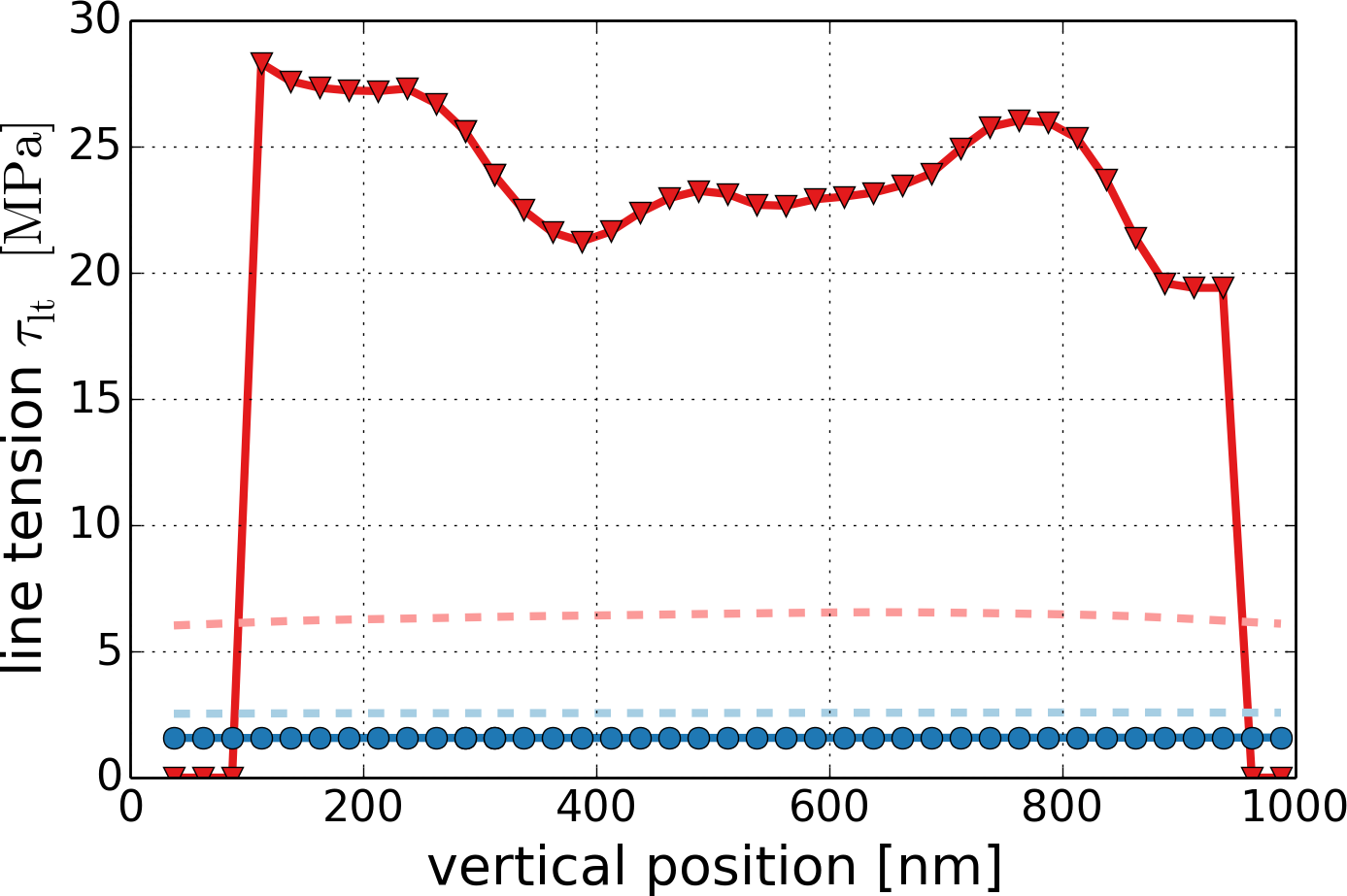
(j) line tension

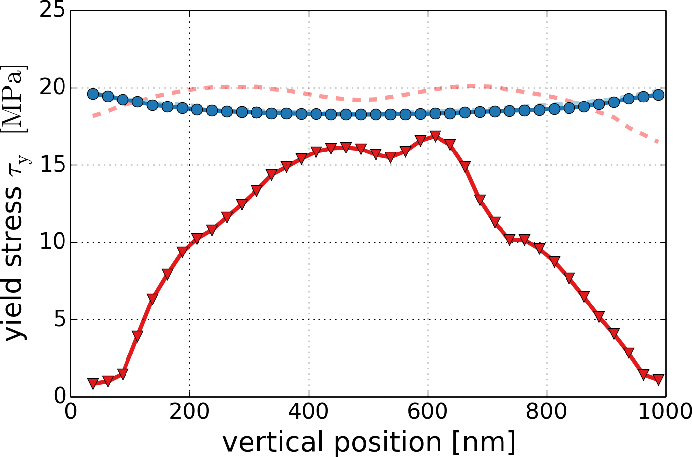
(k) yield stress

(l) velocity

Figure 12: Profiles of CDD field variables along a center slip plane for single slip (a-f) and double slip (g-l) configuration. Density values and plastic slip for the double slip configuration (g)-(i) were multiplied by a factor of 2 to make them comparable with the single slip configuration.

Bibliography

Bibliography

- Acharya and Fressengeas (2012) Acharya, A., Fressengeas, C., 2012. Coupled phase transformations and plasticity as a field theory of deformation incompatibility. International Journal of Fracture 174, 87–94.
- Arsenlis et al. (2007) Arsenlis, A., Cai, W., Tang, M., Rhee, M., Oppelstrup, T., Hommes, G., Pierce, T. G., Bulatov, V. V., 2007. Enabling strain hardening simulations with dislocation dynamics. Modelling and Simulation in Materials Science and Engineering 15, 553–595.
- Arsenlis et al. (2004) Arsenlis, A., Parks, D. M., Becker, R., Bulatov, V. V., 2004. On the evolution of crystallographic dislocation density in non-homogeneously deforming crystals. Journal of the Mechanics and Physics of Solids 52 (6), 1213–1246.
- Arzt (1998) Arzt, E., 1998. Size effects in materials due to microstructural and dimensionalconstraints: a comparative review. Acta Materialia 46 (16), 5611–5626.
- Ashby (1970) Ashby, M., 1970. The deformation of plastically non-homogeneous materials. Philosophical Magazine 21, 399–424.
- Basinski and Basinski (1979) Basinski, S., Basinski, Z., 1979. Dislocations in Solids: Plastic Deformation and Work Hardening. Vol. 4. North-Holland, Amsterdam,.
- Bilby et al. (1955) Bilby, B. A., Bullough, R., Smith, E., 1955. Continuous distributions of dislocations: A new application of the methods of non-riemannian geometry. Proceedings of the Royal Society of London. Series A 231, 263–273.
- Bulatov and Cai (2002) Bulatov, V. V., Cai, W., 2002. Nodal effects in dislocation mobility. Physical Review Letters 89 (11), 115501 1–4.
- Deshpande et al. (2005) Deshpande, V., Needleman, A., Van der Giessen, E., 2005. Plasticity size effects in tension and compression of single crystals. Journal of the Mechanics and Physics of Solids 53 (12), 2661–2691.
- Devincre and Kubin (1997) Devincre, B., Kubin, L. P., 1997. Mesoscopic simulations of dislocations and plasticity. Materials Science and Engineering: A 8, 234–236.
- Ebrahimi et al. (2014) Ebrahimi, A., Monavari, M., Hochrainer, T., 2014. Numerical implementation of continuum dislocation dynamics with the discontinuous Galerkin method. Materials Research Society Symposium Proceedings 1651.
- El-Azab (2000) El-Azab, A., 2000. Statistical mechanics treatment of the evolution of dislocation distributions in single crystals. Physical Review B 61 (18), 11956–11966.
- El-Azab et al. (2007) El-Azab, A., Deng, J., Tang, M., 2007. Statistical characterization of dislocation ensembles. Philosophical Magazine 87, 1201–1223.
- Engels et al. (2012) Engels, P., Ma, A., Hartmaier, A., 2012. Continuum simulation of the evolution of dislocation densities during nanoindentation. International Journal of Plasticity 38 (0), 159–169.
- Fertig and Baker (2009) Fertig, R. S., Baker, S. P., 2009. Simulation of dislocations and strength in thin films: A review. Progress in Materials Science 54 (6), 874–908.
- Fivel et al. (1997) Fivel, M., Verdier, M., Ganova, G., 1997. 3d simulation of a nanoindentation test at a mesoscopic scale. Materials Science and Engineering: A 234-236, 923–926.
- Fleck et al. (1994) Fleck, N., Muller, G., Ashby, M., Hutchinson, J., 1994. Strain gradient plasticity - theory and experiment. Acta Metallurgica et Materialia 42 (2), 475–487.
- Foreman (1967) Foreman, A., 1967. Bowing of a dislocation segment. Philosophical Magazine 15 (137), 1011–1021.
- Fredriksson and Gudmundson (2005) Fredriksson, P., Gudmundson, P., 2005. Size-dependent yield strength of thin films. International Journal of Plasticity 21 (9), 1834–1854.
- Gao and Huang (2003) Gao, H., Huang, Y., 2003. Geometrically necessary dislocation and size-dependent plasticity. Scripta Materialia 48 (2), 113–118.
- Ghoniem et al. (2000) Ghoniem, N. M., Tong, S., Sun, L., 2000. Parametric dislocation dynamics: A thermodynamics-based approach to investigations of mesoscopic plastic deformation. Physical Review B 61 (2), 913.
- Greer and De Hosson (2011) Greer, J. R., De Hosson, J. T. M., 2011. Plasticity in small-sized metallic systems: Intrinsic versus extrinsic size effect. Progress in Materials Science 56 (6), 654–724.
- Groma (1997) Groma, I., 1997. Link between the microscopic and mesoscopic length-scale description of the collective behavior of dislocations. Physical Review B 56 (10), 5807–5813.
- Groma et al. (2003) Groma, I., Csikor, F., Zaiser, M., 2003. Spatial correlations and higher-order gradient terms in a continuum description of dislocation dynamics. Acta Materialia 51, 1271–1281.
- Gurtin (2002) Gurtin, M. E., 2002. A gradient theory of single-crystal viscoplasticity that accounts for geometrically necessary dislocations. Journal of the Mechanics and Physics of Solids 50 (1), 5–32.
- Hesthaven and Warburton (2008) Hesthaven, J. S., Warburton, T., 2008. Nodal discontinuous Galerkin methods. Vol. 54 of Texts in Applied Mathematics. Springer, New York.
- Hirschberger et al. (2011) Hirschberger, C. B., Peerlings, R. H. J., Brekelmans, W A M andGeers, M. G. D., 2011. On the role of dislocation conservation in single-slip crystal plasticity. Modelling and Simullation in Materials Scicience and Engineering 19.
- Hochbruck et al. (2015) Hochbruck, M., Pažur, T., Schulz, A., Thawinan, E., Wieners, C., 2015. Efficient time integration for discontinuous Galerkin approximations of linear wave equations. Zeitschrift fur Angewandte Mathematik und Mechanik 95 (3), 237–259.
- Hochrainer (2006) Hochrainer, T., 2006. Evolving systems of curved dislocations: Mathematical foundations of a statistical theory. Ph.D. thesis, University of Karlsruhe, IZBS.
- Hochrainer et al. (2014) Hochrainer, T., Sandfeld, S., Zaiser, M., Gumbsch, P., 2014. Continuum dislocation dynamics: towards a physical theory of crystal plasticity. Journal of the Mechanics and Physics of Solids 63, 167–178.
- Hochrainer et al. (2007) Hochrainer, T., Zaiser, M., Gumbsch, P., 2007. A three-dimensional continuum theory of dislocation systems: kinematics and mean-field formulation. Philosophical Magazine 87 (8-9), 1261–1282.
- Hochrainer et al. (2009) Hochrainer, T., Zaiser, M., Gumbsch, P., 2009. Dislocation transport and line length increase in averaged descriptions of dislocations. AIP Conference Proceedings 1168 (1), 1133–1136.
- Jerusalem et al. (2012) Jerusalem, A., Fernandez, A., Kunz, A., Greer, J. R., 2012. Continuum modeling of dislocation starvation and subsequent nucleation in nano-pillar compressions. Scripta Materialia 66 (2), 93–96.
- Kondo (1952) Kondo, K., 1952. On the geometrical and physical foundations of the theory of yielding. Proceedings of the 2nd Japan National Congress for Applied Mechechanics, 41–47.
- Kosevich (1979) Kosevich, A. M., 1979. Crystal dislocations and the theory of elasticity. In: Nabarro, F. R. (Ed.), Dislocations in Solids. Vol. 1. North Holland, Amsterdam, pp. 33–141.
- Kratochvil et al. (2007) Kratochvil, J., Kruzik, M., Sedlacek, R., 2007. Statistically based continuum model of misoriented dislocation cell structure formation. Physical Reviews B 75 (6), 064104–1 – 064104–14.
- Kröner (1955) Kröner, E., 1955. Der fundamentale zusammenhang zwischen versetzungsdichte und spannungsfunktion. Zeitschrift für Physik 142, 463–475.
- Kröner (1958) Kröner, E., 1958. Kontinuumstheorie der Versetzungen und Eigenspannungen. Springer.
- Kubin and Canova (1992) Kubin, L., Canova, G., 1992. The modeling of dislocation patterns. Scripta Metallurgica et Materialia 27 (8), 957–962.
- Kubin et al. (2008) Kubin, L., Devincre, B., Hoc, T., 2008. Modeling dislocation storage rates and mean free paths in face-centered cubic crystals. Acta Materialia 56, 6040–6049.
- Le and Günther (2014) Le, K., Günther, C., 2014. Nonlinear continuum dislocation theory revisited. International Journal of Plasticity 53 (0), 164–178.
- Leung et al. (2015) Leung, H., Leung, P., Cheng, B., Ngan, A., 2015. A new dislocation-density-function dynamics scheme for computational crystal plasticity by explicit consideration of dislocation elastic interactions. International Journal of Plasticity 67 (0), 1–25.
- Li et al. (2014) Li, D., Zbib, H., Sun, X., Khaleel, M., 2014. Predicting plastic flow and irradiation hardening of iron single crystal with mechanism-based continuum dislocation dynamics. International Journal of Plasticity 52 (0), 3–17, in Honor of Hussein Zbib.
- Liu et al. (2011) Liu, Z., Zhuang, Z., Liu, X., Zhao, X., Zhang, Z., 2011. A dislocation dynamics based higher-order crystal plasticity model and applications on confined thin-film plasticity. International Journal of Plasticity 27 (2), 201–216.
- Monavari et al. (2014) Monavari, M., Zaiser, M., Sandfeld, S., 2014. Comparison of closure approximations for continuous dislocation dynamics. Materials Research Society Symposium Proceedings 1651.
- Nix and Gao (1998) Nix, W. D., Gao, H., 1998. Indentation size effects in crystalline materials: A law for strain gradient plasticity. Journal of the Mechanics and Physics of Solids 46 (3), 411–425.
- Nye (1953) Nye, J., 1953. Some geometrical relations in dislocated crystals. Acta Metallurgica 1, 153–162.
- Orowan (1934) Orowan, E., 1934. Zur Kristallplastizität. Zeitschrift für Physik 89, 605–659.
- Orowan (1940) Orowan, E., 1940. Problems of plastic gliding. Proceedings of the Physical Society 52 (1), 8.
- Po et al. (2014) Po, G., Mohamed, M. S., Crosby, T., Erel, C., El-Azab, A., Ghoniem, N. M., 2014. Recent progress in discrete dislocation dynamics and its applications to micro plasticity. The Journal of The Minerals, Metals & Materials Society, 1–13.
- Polanyi (1934) Polanyi, M., 1934. Über eine Art Gitterstörung, die einen Kristall plastisch machen könnte. Zeitschrift für Physik 89, 660–664.
- Reuber et al. (2014) Reuber, C., Eisenlohr, P., Roters, F., Raabe, D., 2014. Dislocation density distribution around an indent in single-crystalline nickel: Comparing nonlocal crystal plasticity finite-element predictions with experiments. Acta Materialia 71 (0), 333–348.
- Sandfeld (2010) Sandfeld, S., 2010. The evolution of dislocation density in a higher-order continuum theory of dislocation plasticity. Shaker Verlag Aachen, Germany.
- Sandfeld and Hochrainer (2011) Sandfeld, S., Hochrainer, T., 2011. Towards Frank-Read sources in the continuum dislocation dynamics theory. AIP Conference Proceedings 1389.
- Sandfeld et al. (2010) Sandfeld, S., Hochrainer, T., Zaiser, M., Gumbsch, P., 2010. Numerical implementation of a 3d continuum theory of dislocation dynamics and application to microbending. Philosophical Magazine 90 (27), 3697–3728.
- Sandfeld et al. (2011) Sandfeld, S., Hochrainer, T., Zaiser, M., Gumbsch, P., 2011. Continuum modeling of dislocation plasticity: Theory, numerical implementation and validation by discrete dislocation simulations. Journal of Materials Research 26 (5), 623–632.
- Sandfeld et al. (2013) Sandfeld, S., Monavari, M., Zaiser, M., 2013. From systems of discrete dislocations to a continuous field description: stresses and averaging aspects. Modelling and Simulation in Materials Science and Engineering 21 (8), 085006.
- Sandfeld et al. (2015) Sandfeld, S., Verbeke, V., Devincre, B., 2015. Orientation-dependent pattern formation in a 1.5d continuum model of curved dislocations. Materials Research Society Symposium Proceedings 1755.
- Scardia et al. (2014) Scardia, L., Peerlings, R., Peletier, M., Geers, M., 2014. Mechanics of dislocation pile-ups: A unification of scaling regimes. Journal of the Mechanics and Physics of Solids 70 (1), 42–61.
- Schulz et al. (2014) Schulz, K., Schmitt, S., Dickl, D., Sandfeld, S., Weygand, D., Gumbsch, P., 2014. Analysis of dislocation pile-ups using a dislocation-based continuum theory. Modelling and Simulation in Materials Science and Engineering 22 (2), 025008.
- Schwarz et al. (2005) Schwarz, C., Sedlacek, R., Werner, E., 2005. Application of a continuum dislocation-based model to a tensile test on a thin film. Materials Science and Engineering: A 400, 443–447, Intenational Conference on Fundamentals of Plastic Deformation, La Colle sur Loup, France, Sep. 13-17, 2004.
- Sedláček et al. (2003) Sedláček, R., Kratochvíl, J., Werner, E., 2003. The importance of being curved. Philosophical Magazine 83 (31-34), 3735–3752.
- Sedláček et al. (2003) Sedláček, R., Kratochvíl, J., Werner, E., 2003. The importance of being curved: bowing dislocations in a continuum description. Philosophical Magazine 83 (31-34), 3735–3752.
- Shan et al. (2008) Shan, Z. W., Mishra, R. K., Syed Asif, S. A., Warren, O. L., Minor, A. M., 2008. Mechanical annealing and source-limited deformation in submicrometre-diameter ni crystals. Nature Materials 7 (2), 115–119.
- Stolken and Evans (1998) Stolken, J., Evans, A., 1998. A microbend test method for measuring the plasticity length scale. Acta Materialia 46, 5109–5115.
- Taupin et al. (2013) Taupin, V., Capolungo, L., Fressengeas, C., Das, A., Upadhyay, M., 2013. Grain boundary modeling using an elasto-plastic theory of dislocation and disclination fields. Journal of the Mechanics and Physics of Solids 61 (2), 370–384.
- Taylor (1934a) Taylor, G., 1934a. The mechanism of plastic deformation of crystals. Proceedings of the Royal Society of London. Series A, Mathematical and Physical Sciences 145, 362–415.
- Taylor (1934b) Taylor, G. I., 1934b. The mechanism of plastic deformation of crystals. part I. theoretical. Proceedings of the Royal Society of London A: Mathematical, Physical and Engineering Sciences 145 (855), 362–387.
- Wallin et al. (2008) Wallin, M., Curtin, W., Ristinmaa, M., Needleman, A., 2008. Multi-scale plasticity modeling: Coupled discrete dislocation and continuum crystal plasticity. Journal of the Mechanics and Physics of Solids 56 (11), 3167–3180.
- Weygand et al. (2002) Weygand, D., Friedman, L. H., van der Giessen, E., Needleman, A., 2002. Aspects of boundary-value problem solutions with three-dimensionaldislocation dynamics. Modelling and Simulation in Materials Science and Engineering 10, 437–468.
- Weygand and Gumbsch (2005) Weygand, D., Gumbsch, P., 2005. Study of dislocation reactions and rearrangements under different loading conditions. Modelling and Simulation in Engineering 400-401, 158–161.
- Wulfinghoff and Böhlke (2015) Wulfinghoff, S., Böhlke, T., 2015. Gradient crystal plasticity including dislocation-based work-hardening and dislocation transport. International Journal of Plasticity, http://dx.doi.org/10.1016/j.ijplas.2014.12.003.
- Xiang (2009) Xiang, Y., 2009. Continuum approximation of the Peach-Koehler force on dislocations in a slip plane. Journal of the Mechanics and Physics of Solids 57 (4), 728–743.
- Xiong et al. (2012) Xiong, L., Deng, Q., Tucker, G., McDowell, D. L., Chen, Y., 2012. A concurrent scheme for passing dislocations from atomistic to continuum domains. Acta Materialia 60 (3), 899–913.
- Yefimov et al. (2004) Yefimov, S., Groma, I., van der Giessen, E., 2004. A comparison of a statistical-mechanics based plasticity model with discrete dislocation plasticity calculations. J. Mech. and Phys. Solids 52 (2), 279 – 300.
- Zaiser and Hochrainer (2006) Zaiser, M., Hochrainer, T., 2006. Some steps towards a continuum representation of 3d dislocation systems. Scripta Materialia 54 (5), 717–721.
- Zaiser et al. (2001) Zaiser, M., Miguel, M.-C., Groma, I., 2001. Statistical dynamics of dislocation systems: The influence of dislocation-dislocationcorrelations. Physical Review B 64, 224102.
- Zaiser et al. (2007) Zaiser, M., Nikitas, N., Hochrainer, T., Aifantis, E., 2007. Modelling size effects using 3d density-based dislocation dynamics. Philosophical Magazine 87, 1283–1306.
-
Zaiser and Sandfeld (2014)
Zaiser, M., Sandfeld, S., 2014. Scaling properties of dislocation simulations
in the similitude regime. Modelling and Simulation in Materials Science and
Engineering 22 (6).
URL http://iopscience.iop.org/0965-0393/22/6/065012/ - Zhang et al. (2014) Zhang, X., Aifantis, K. E., Ngan, A. H., 2014. Interpreting the stress-strain response of al micropillars through gradient plasticity. Materials Science and Engineering: A 591 (0), 38–45.
- Zhou et al. (2010) Zhou, C. Z., Biner, S. B., LeSar, R., 2010. Discrete dislocation dynamics simulations of plasticity at small scales. Acta Materialia 58, 1565–1577.
- Zhu et al. (2014) Zhu, Y., Wang, H., Zhu, X., Xiang, Y., 2014. A continuum model for dislocation dynamics incorporating Frank-Read sources and Hall-Petch relation in two dimensions. International Journal of Plasticity 60 (0), 19–39.