Range optimized theory of electron liquids with application to the homogeneous gas

Abstract

A simple optimization scheme is used to compute the density-density response function of an electron liquid. Higher order terms in the perturbation expansion beyond the random phase approximation are summed approximately by enforcing the constraint that the spin density pair correlation functions be positive. The theory is applied to the 3-D homogeneous electron gas at zero temperature. Quantitative comparison is made with previous theory and data from quantum Monte Carlo simulation. When thermodynamic consistency is enforced on the compressibility, agreement with the available simulation data is very good for the entire paramagnetic region, from weakly to strongly correlated densities. In this case, the accuracy of the theory is comparable to or better than the best of previous theory, including the full GW approximation. In addition, it is found that the spin susceptibility diverges at a lower density ($r_{s}\approx 107$) than the current estimate for the liquid-solid transition. Application of the theory to inhomogeneous electron liquids is discussed.

I Introduction

In many practical calculations of electronic structure, such as for semiconductors and molecules, the density-density response function $\chi$ plays a central role. The popular Kohn-Sham electronic density functional theory (DFT)Kohn (1999); Perdew and Kurth (2003); Capelle (2006), and Hedin’s “GW” approximation (GWA) of many-body perturbation theoryHedin (1965); Aulbur et al. (2000) are two such methods that use $\chi$.

In DFT, $\chi$ is an important ingredient in the exchange-correlation functional, $E_{xc}$, which is the main object for approximations in the theory.Perdew and Kurth (2003) The workhorse local density approximation (LDA) and its generalizations avoid explicitly estimating $\chi$ for the inhomogeneous liquid. Instead, they approximate $E_{xc}$ by relying on knowing the correlations of a simpler system, the homogeneous electron gas, i.e, jellium.Giuliani and Vignale (2005) The correlations of this latter system have been computed accurately using theory and quantum Monte Carlo (QMC) simulation.Gorobchenko et al. (1989) While being very accurate for the electron structure of molecules and electron density of many systems, DFT-LDA and its variants have the limitation of not being able to describe accurately band gaps, nor London dispersion (i.e., van der Waals) interactions very well.Perdew and Kurth (2003) The former is crucial to understanding the properties of semiconductors, while the latter is important to understanding weakly bonded systems, such as water. A recent branch of DFT uses the adiabatic-connection fluctuation-dissipation form for the correlation energy, which is the troublesome part of $E_{xc}$. In this branch there is much current interest in the use of the random phase approximation (RPA) for $\chi$.Angyan et al. (2011) Unlike the LDA, this DFT-RPA does predict reasonable band gaps for many solids,Niquet and Gonze (2004) and, with some extra effort, reasonable London dispersion interactions between atoms.Toulouse et al. (2009); Klimes and Michaelides (2012)

In GWA, $\chi$ enters through the screened potential $W$ to compute ultimately the one-particle Green’s function, $G$, from which the band structure is extracted.Hedin (1965); Giuliani and Vignale (2005) In perturbative calculations around a DFT reference state, known as “one-shot GW,” $\chi$ is almost always taken to have a simple RPA form. In the full version of GWA, $\chi$ is computed in a self-consistent loop along with $G$. Being able to predict accurate band structure for many solids, GWA has rapidly become one of the main methods for computing the electronic structure of crystalline materials.Bruneval et al. (2006); Yu and Cardona (2010) A drawback to this approach though is that the full, self-consistent solution often does not improve the predictions of the theory, and can make it worse.Holm and von Barth (1998) Application of the GWA to jellium has shown that the main weakness is the expression for $\chi$ obtained from $G$.Holm and von Barth (1998)

For both approaches then, a better way to compute $\chi$ would be very desired. In this paper, a simple scheme called range optimization is described that goes beyond the RPA for $\chi$ to accomplish this task. Range optimization was originally used to improve the RPA theory of classical molecules. This “range-optimized” RPA (RO-RPA) theory was able to describe very well the equilibrium structure and thermodynamics of strongly charged polyelectrolyte solutions.Donley et al. (2004, 2005); Donley and Heine (2006) It has also been applied successfully to the study of the hydrated electron.Donley et al. (2014) Given that a number of weaknesses of the GWA became apparent only after the full version had been implemented for jellium, it is important for the theory here to be analyzed first for that system. This is the intent of the present paper. As will be shown below, the scheme applied to jellium greatly improves the predictions of the theory over the basic RPA. A new algorithm to implement range optimization, valid for inhomogeneous liquids, is also described here.

II Theory

Let the analysis be confined to a homogeneous electron gas, i.e., jellium, in 3-D at zero temperature in the paramagnetic phase. As a reminder, jellium has a balancing background of positive charge that is uniform and rigid.Fetter and Walecka (2003); Giuliani and Vignale (2005)

The theory here is centered around the time-ordered, spin density-density response function (or spin polarization propagator), $\chi_{ij}(x,x^{\prime})$, where $i$ and $j$ label the spin ($\uparrow$ and $\downarrow$), and $x\equiv\{{\bf r},t\}$, with ${\bf r}$ being the position and $t$ the time. It is defined as:

$$\chi_{ij}(x,x^{\prime})={1\over i\hbar}{\langle\Psi_{0}|T[\delta{\hat{n}}_{i}(x)\delta{\hat{n}}_{j}(x^{\prime})]|\Psi_{0}\rangle\over\langle\Psi_{0}|\Psi_{0}\rangle}.$$ (II.1)

Here, $|\Psi_{0}\rangle$ is the system ground state, and $T$ denotes the time ordered product. Also,

$$\delta{\hat{n}}_{i}(x)={\hat{n}}_{i}(x)-\langle{\hat{n}}_{i}(x)\rangle,$$ (II.2)

where ${\hat{n}}_{i}(x)$ is the number density operator in the Heisenberg representation for spin $i$ electrons at point $x$,Fetter and Walecka (2003) and $\langle{\hat{n}}_{i}(x)\rangle$ denotes its ground state average. For the paramagnetic phase, $\langle{\hat{n}}_{\uparrow}(x)\rangle=\langle{\hat{n}}_{\downarrow}(x)\rangle=n/2$, where $n$ is the average electron density.

Jellium is translationally invariant and $\chi$ is symmetric with respect to $x\leftrightarrow x^{\prime}$, so $\chi_{ij}(x,x^{\prime})\rightarrow\chi_{ij}(r,\tau)$, where $r=|{\bf r}-{\bf r}^{\prime}|$ and $\tau=t-t^{\prime}$. For this case, it is helpful to work with the dual Fourier transform, $\chi_{ij}(k,\omega)$, $k=|{\bf k}|$ being the wavevector and $\omega$ the frequency.

A number of useful quantities can be obtained from $\chi_{ij}(k,\omega)$.Giuliani and Vignale (2005) First is the system compressibility $K$:

$${K_{0}\over K}=-N(0)\lim_{k\rightarrow 0}\left[{1\over\chi(k,0)}+v(k)\right],$$ (II.3)

where $\chi(k,\omega)=\sum_{ij}\chi_{ij}(k,\omega)$ is the total density-density response function, and $N(0)=mk_{F}/(\pi^{2}\hbar^{2})$, with $m$ being the electron mass, and $k_{F}=(3\pi^{2}n)^{1/3}$ being the Fermi wavevector.Giuliani and Vignale (2005) Also, $K_{0}$ is the compressibility of the non-interacting gas, and $v(k)$ is the Fourier transform of the electron-electron Coulomb potential, $v(r)=e^{2}/r$, with $e$ being the electron charge. Second is the spin susceptibility $\chi_{S}$:

$${\chi_{P}\over\chi_{S}}=-N(0)\lim_{k\rightarrow 0}\left[{1\over 2(\chi_{\uparrow\uparrow}(k,0)-\chi_{\uparrow\downarrow}(k,0))}\right],$$ (II.4)

where $\chi_{P}$ is the spin susceptibility of the non-interacting gas. Third are the partial static structure factors:

$$S_{ij}(k)={2i\hbar\over\pi n}\int_{0}^{\infty}d\omega\chi_{ij}(k,\omega),$$ (II.5)

which are real, and have exploited that $\chi_{ij}(k,\omega)$ is symmetric about $\omega=0$. Fourth are the spin-spin pair correlation (or radial distribution) functions:

$$g_{ij}(r)=1+{2\over n}\int{d{\bf k}\over(2\pi)^{3}}\bigl{[}S_{ij}(k)-\delta_{ij}\bigr{]}exp(i{\bf k}\cdot{\bf r}),$$ (II.6)

where $\delta_{ij}$ is the Kronecker delta. The pair correlation function $g_{ij}(r)$ is proportional to the equilibrium probability density of there being an electron of spin $j$ a distance $r$ from one with spin $i$ at the same time. As a density, $g_{ij}(r)$ is strictly positive for all $r$. Last, the correlation energy $E_{corr}$ can be obtained from $S_{ij}(k)$.Fetter and Walecka (2003) Two expressions for $E_{corr}$ were used and they are given in Sec. III below.

Define the matrix inverse of $\chi_{ij}(k,\omega)$ by $\sum_{s}\chi_{is}(k,\omega)\chi_{sj}^{-1}(k,\omega)=\delta_{ij}$. This inverse can be represented exactly as:

$$\chi_{ij}^{-1}(k,\omega)={\tilde{\chi}}_{ij}^{-1}(k,\omega)-v_{ij}(k),$$ (II.7)

where $v_{ij}(k)=v(k)$, and ${\tilde{\chi}}_{ij}(k,\omega)$ is the proper spin density-density response function (or proper spin polarization propagator).Fetter and Walecka (2003); Giuliani and Vignale (2005) It is helpful to rewrite Eq.(II.7) as:

$$\chi_{ij}^{-1}(k,\omega)=\chi_{0ij}^{-1}(k,\omega)-v_{ij}(k)-u_{ij}(k,\omega),$$ (II.8)

where $u_{ij}(k,\omega)=\chi_{0ij}^{-1}(k,\omega)-{\tilde{\chi}}_{ij}^{-1}(k,\omega)$ and $\chi_{0ij}(k,\omega)=\delta_{ij}\chi_{0}(k,\omega)/2$, with $\chi_{0}(k,\omega)$ being the total density-density response function of the non-interacting gas, i.e., the Lindhard function. This Lindhard function can be computed analytically.Fetter and Walecka (2003)

Setting $u_{ij}(k,\omega)$ to zero reduces Eq.(II.8) to the familiar RPA expression for $\chi_{ij}$.Giuliani and Vignale (2005) As is well known, the RPA tends to work well if the interactions are weak. However, for strongly interacting systems it works less well, causing, for example, the pair correlation functions $g_{ij}(r)$ to be (very) negative at small $r$.

More recent research on jellium has steadily improved upon the RPA. Almost all of these theories have worked with the one-component expression for the total density-density response function, $\chi(k,\omega)$, by developing accurate approximations to the static and dynamic local field factors, $G_{+}(k)$ and $G_{+}(k,\omega)$, respectively. These are defined by:

$$\chi^{-1}(k,\omega)=\chi_{0}^{-1}(k,\omega)-v(k)[1-G_{+}],$$ (II.9)

where $G_{+}$ denotes $G_{+}(k)$ or $G_{+}(k,\omega)$. In this manner, the one-component optimized potential, $u=-vG_{+}$.

The best of these theories now agree with QMC simulation data for the paramagnetic state for the correlation energy $E_{corr}$ within a few percent for the density range of most metals, $2<r_{s}<6$.Vosko et al. (1980); Gorobchenko et al. (1989) Here, $r_{s}=r_{0}/a_{0}=1/(\alpha k_{F}a_{0})$, where $r_{0}=({3/(4\pi n)})^{1/3}$ is the average distance between electrons, $a_{0}$ is the Bohr radius, and $\alpha=(4/(9\pi))^{1/3}$. A limitation of these theories though is that they usually apply only to the paramagnetic, i.e., zero polarization state. This local field factor approach can be extended to examine partially polarized states, and thus give information about the jellium phase diagram.Tanaka and Ichimaru (1989) However, the cost is an increase in the complexity of the theory. As such, a different path will be taken here.

To go beyond the RPA for the multi-component model, Eq.(II.8), the range optimization scheme will be used. This scheme has been described in detail elsewhere,Donley et al. (2004, 2005) but a summary is given here.

The aim is to approximate the higher order terms embodied in $u_{ij}(k,\omega)$ in some manner. First, let $u_{ij}(k,\omega)$ be independent of frequency $\omega$. This approximation is not necessary, but is a sensible one for computing the static equilibrium properties of the gas, such as $g_{ij}(r)$ and $E_{corr}$. Next, let $u_{ij}(k)$ be real. This follows the common assumption that the static local field factor $G_{+}(k)$ is dominated by its real part.Giuliani and Vignale (2005) In this manner, the inverse Fourier transform of $u_{ij}(k)$, $u_{ij}(r)$, can be viewed as a short-ranged attractive potential that counteracts the strong electron-electron Coulomb repulsion in $v(r)$ at small $r$. What then is $u_{ij}(r)$?

Now, the RPA works well at high density, $r_{s}<1$, where the kinetic energy and exchange interactions dominate the Coulomb repulsion. At low density, $r_{s}\gg 1$, where the RPA breaks down, the electron-electron Coulomb repulsion causes $g_{ij}(r)$ to be essentially zero out to some range $\sigma_{ij}$ (see Figure 1). Notice though that if $g_{ij}(r)$ were zero, it makes little difference to the electrons that the repulsion at that distance were infinite as opposed to just very large. As such, replace the Coulomb potential with a hard-core one for distances $r<\sigma_{ij}$. While the RPA fails for hard-core potentials naturally, methods developed in the classical theory of liquids have found ways to overcome this problem.Hansen and McDonald (1986) One is the mean spherical approximation (MSA) closure.Lebowitz and Percus (1966)

Applied to jellium, the MSA states that if $\sigma_{ij}$ is the range of the hard-core potential between electrons of spin $i$ and $j$, then $g_{ij}(r)$ is zero inside this range. But since $g_{ij}(r)$ is zero inside, the equations relating $u_{ij}(r)$ to $g_{ij}(r)$ can be used to determine $u_{ij}(r)$ inside. That is, $u_{ij}(r)$ takes whatever form is needed to ensure that $g_{ij}(r)$ is zero inside the core. The closure is summarized as:

$$g_{ij}(r) =0,\ r<\sigma_{ij},$$

$$u_{ij}(r) =0,\ r>\sigma_{ij}.$$ (II.10)

This closure, along with Eqs. (II.5), (II.6) and (II.8), form a closed set of equations for $g_{ij}(r)$ and $u_{ij}(r)$, assuming the $\sigma_{ij}$ are known. The last step is to optimize the range, $\sigma_{ij}$, by letting it have the smallest value such that $g_{ij}(r)$ is positive for all $r$. Since the theory will now work properly for low and high densities, it presumably will work well for intermediate densities as well. This set of self-consistent equations will be referred to as RO-RPA theory.

There are at least two ways to compute the compressibility: by the structure route using $\chi(k,0)$ in Eq.(II.3), and by the energy route using an expression for the total energyGiuliani and Vignale (2005). Since the RO-RPA theory is approximate, the structure and energy routes will not give the same value for $K$. It is well known though that enforcing consistency between these two routes, i.e., enforcing the “sum rule”, can improve a theory, often greatly.Dickman and Stell (1996) This thermodynamic consistency can be attained under range optimization by noticing that $g_{ij}(r)$ need not be set to zero inside the core. Instead, the minimum of $g_{ij}(r)$ could have a non-zero value, $g_{0}$. The MSA closure can then be generalized to:

$$g_{ij}(r) =g_{0},\ r<\sigma_{ij},$$

$$u_{ij}(r) =0,\ r>\sigma_{ij},$$ (II.11)

where the value of $g_{0}$ is determined by enforcing the sum rule on the compressibility. This extra condition, along with the RO-RPA equations above, will be referred to as “thermodynamically consistent” RO-RPA (TCRO-RPA) theory.

III Numerical solution

All theories were solved numerically as follows. Functions of $r$ or $k$ were solved on a grid of $N_{r}$ points with spacing $\Delta r$ or $\Delta k=\pi/(N_{r}\Delta r)$, respectively. Unless stated otherwise, $N_{r}$ and $\Delta r$ were set to $2^{11}$ and $0.05/k_{F}$, respectively. To compute the static structure factor $S_{ij}(k)$, the integration of $\chi_{ij}(k,\omega)$ over $\omega$ given by Eq.(II.5) was performed along the positive real axis. It is well known that along the real axis, a contribution to $S_{ij}(k)$ from the plasmon mode must be accounted forPines and Nozieres (1999); Giuliani and Vignale (2005) and that was done. As a check though, the integration was also performed along the positive imaginary axis.Pines and Nozieres (1999); Hedin (1965) In either case, the integral over frequency was evaluated using Romberg integrationPress et al. (1992) with the relative error tolerance being $10^{-6}$ and $10^{-9}$ for the real and imaginary axis cases, respectively.

Once $S_{ij}(k)$ was computed, the integral over $k$ in Eq.(II.6) was evaluated by inverse Fourier transform to obtain $g_{ij}(r)$. As a check on the accuracy, the RPA values for $g_{ij}(0)$ were computed. It was found that unlike the correlation energy, $E_{corr}$, $g_{ij}(0)$ was sensitive to the grid spacing, but setting $N_{r}=2^{16}$ and $\Delta r=0.05/(32k_{F})$ gave convergent RPA values of $g_{ij}(0)$ within $0.1\%$. The grid spacing did not affect greatly any other quantity, though for increased accuracy in determining the density at which the spin susceptibility $\chi_{S}$ diverged, $N_{r}$ and $\Delta r$ were set to $2^{13}$ and $0.0125/k_{F}$, respectively, for $r_{s}\geq 70$.

A new algorithm was used to implement range optimization. This new algorithm has two advantages over the one used in past workDonley et al. (2004, 2005); Donley and Heine (2006); Donley et al. (2014): it is straightforward to apply to inhomogeneous liquids, and is more efficient even for jellium. It is as follows: 1) An initial guess is made for the optimized potentials $u_{ij}(r)$, which could be zero. 2) With the $u_{ij}(r)$, the theory is solved as described above for the pair correlation functions $g_{ij}(r)$. 3) The difference $\Delta g_{ij}(r)=g_{ij}(r)-g0$ is computed for all $r$, where $g0=0$ for standard range optimization. 4) As a variation on Picard iterationHansen and McDonald (1986), the change in the value of the optimized potential is set to $\alpha\Delta g_{ij}(r)$, with the mixing parameter $\alpha\leq 0.25$. 5) Since the optimized potential is an attractive potential, its new value for each $r$ is checked to determine if it is greater than zero; if so, it is set to zero. 6) The difference between the new and old values is checked to determine if the potential has converged; if not, the steps starting at 2) are repeated until convergence is obtained. Here, the relative error tolerance on each point of $u_{ij}(r)$ was $10^{-4}$, although in some cases it was reduced to $10^{-5}$ as a check.

Note that in this algorithm the optimized ranges, $\sigma_{ij}$, are not considered explicitly. Instead, the algorithm relies on knowing only the value of the pair correlation function, $g_{ij}$, to obtain a refined guess for the optimized potential, $u_{ij}$, at the same point. In that way, the above algorithm can be used for inhomogeneous liquids by the mere replacement of $g_{ij}(r)$ and $u_{ij}(r)$ with $g_{ij}({\bf r}_{1},{\bf r}_{2})$ and $u_{ij}({\bf r}_{1},{\bf r}_{2})$, respectively, and then using the inhomogeneous analog of Eq.(II.8).Martin (2004)

For all theories except TCRO-RPA the correlation energy was computed in the usual manner as a charging integral over the coupling constant $e^{2}$, i.e., via the adiabatic-connection fluctuation-dissipation theorem.Fetter and Walecka (2003) Define $\epsilon_{c}=2a_{0}E_{corr}/(Ne^{2})$ as a scaled correlation energy per particle (in units of Rydbergs), with $N$ being total number of electrons. Then this energy equation is:

$$\epsilon_{c}(r_{s})={4\pi\over\alpha r_{s}}\int_{0}^{1}d\lambda\ w(\lambda),$$ (III.1)

where

$$w(\lambda)={1\over 2\pi^{2}k_{F}}\int_{0}^{\infty}dk\left[S(k,\lambda)-S(k,0)\right].$$ (III.2)

Here, $S(k,\lambda)={1/2}\sum_{ij}S_{ij}(k,\lambda)$ is the total structure factor for a gas with electron-electron potential $\lambda v(r)$. The integral over $k$, Eq.(III.2), was computed via quadrature. The charging integral, Eq.(III.1), was computed using Romberg integration with an error tolerance of $10^{-4}$.

Enforcing thermodynamic consistency for the TCRO-RPA theory was done as follows. First, for a given value of $r_{s}$, a value for $g0$ was guessed. Then the optimized potentials, $u_{ij}(r)$, were computed in the same manner as for the RO-RPA. Next, the compressibility was computed using the structure route formula, Eq.(II.3). For the compressibility via the energy route, its value was computed initially using the Perdew-Wang fit for the correlation energy $E_{corr}$,Perdew and Wang (1992) and an expression relating the total energy to the compressibility.Giuliani and Vignale (2005) The change in the value of $g0$ was set proportional to the difference between values of $K_{0}/K$ from these two routes. With this new $g0$, steps 2)-6) above were repeated, and this iteration was continued until the value of $g0$ converged. This procedure was repeated to obtain $\chi_{ij}(k,\omega)$ on a grid for $0\leq r_{s}\leq 11$ (see below) with spacing $\Delta r_{s}=0.1$.

These density-density response functions were then used to compute the correlation energy over this range. The representation of $E_{corr}$ expressed as an integral over $r_{s}$ was used:Singwi et al. (1968); Utsumi and Ichimaru (1980)

$$\epsilon_{c}(r_{s})=\epsilon_{c}^{rpa}(r_{s})-{4\over\pi\alpha r_{s}^{2}}\int_{0}^{r_{s}}dx\Delta\gamma(x),$$ (III.3)

where

$$\Delta\gamma(r_{s})=-{1\over 2k_{F}}\int_{0}^{\infty}dk\left[S(k,r_{s})-S_{rpa}(k,r_{s})\right].$$ (III.4)

Here, $\epsilon_{c}^{rpa}(r_{s})$ and $S_{rpa}(k,r_{s})$ are the RPA values for the correlation energy and total structure factor, respectively, at mean separation $r_{s}$. An accurate interpolation formula for $\epsilon_{c}^{rpa}$ due to Perdew-WangPerdew and Wang (1992) was used here.

The integral, Eq.(III.4), for $\Delta\gamma(r_{s})$ was computed for each $r_{s}$ in the same manner as for Eq.(III.2). The energy route expression for the compressibility consists of derivatives of $\epsilon_{c}$ with respect to $r_{s}$. To minimize errors then, this set of $\Delta\gamma$ values was then fit to an $n$th degree polynomial in $r_{s}$. Degree $n=11$ was found to give a sufficiently accurate fit ($n=9$ worked almost as well). With this functional form, Eq.(III.3) was evaluated analytically. The self-consistent theory for $g_{0}$ was then solved again, with the new and old values for $\epsilon_{c}$ being used to compute the energy route $K$ with a mixture of 1:1 old to new. After new density-density response functions, $\chi_{ij}(k,\omega)$ were computed, the procedure to compute new values for $\epsilon_{c}$ was repeated. It was found that the fitted values for $K$ had converged to within $10^{-3}$ ($10^{-5}$ for $\epsilon_{c}$) for $r_{s}\leq 10$ after seven iterations.

At $r_{s}\approx 0$, $g_{0}\approx 0$ naturally, then $g_{0}$ rose to a maximum of 0.177 at $r_{s}\approx 1.7$, and then gradually dropped to zero again at $r_{s}\approx 10.8$. When the positivity constraint on $g_{ij}(r)$ was relaxed, $g_{0}$ became slightly negative as $r_{s}$ increased beyond 10.8. Since this positivity constraint on $g_{ij}(r)$ is more important than enforcing a sum rule, $r_{s}\approx 10.8$ is then the limit of the usefulness of enforcing thermodynamic consistency on the compressibility. However, it will be shown below that since the RO-RPA is most accurate at low density, this limit is not regarded as important.

For comparison, some results of the theories of Singwi-Tosi-Land-Sjölander (STLS),Singwi et al. (1968) and Utsumi and Ichimaru (UI) Utsumi and Ichimaru (1980) will also be shown. The UI theory is considered accurate for the short range behavior of the pair correlation function at metallic densities.Gorobchenko et al. (1989) The STLS theory is considered accurate for the correlation energy and almost as accurate as UI for the pair correlation function, but is also straightforward to implement. The theory has also been generalized to apply to inhomogeneous liquids in atoms and ions.Gould and Dobson (2012) The STLS theory was solved for the total structure factor $S(k)$ in a similar manner to that of $S_{ij}(k)$ for the RO-RPA. Once $S(k)$ was determined self-consistently, the spin-averaged $g(r)={1/4}\sum_{ij}g_{ij}(r)$ was obtained by inverse Fourier transform using the analog of Eq.(II.6). The UI theory was solved in the same manner as the RPA, but with $v(k)\rightarrow v(k)(1-G_{+}(k))$. Values for the static local field factor $G_{+}(k)$ were interpolated from data presented in Table I of Utsumi and Ichimaru (1980).

IV Results

Unless noted otherwise, all RO-RPA results given here will be for the multi-component version described in Sec.II above. Results of the one- and multi-component versions of the RPA are the same for the quantities examined here.

Figure 1 shows results for the spin-averaged pair correlation function, $g(r)$, for various densities. As a comparison, QMC simulation data of Ceperley and co-workers is also shown.Ceperley and Alder (1980); Zong et al. (2002) As can be seen, the predictions of the RO-RPA are much improved over the RPA, with the RO-RPA outperforming, as expected, the STLS theory at very low density, $r_{s}=50$. For $r_{s}=2$, the contact value, $g(0)=0.176$ and 0.175 for the UI and TCRO-RPA theories, respectively, which are 10% smaller than the simulation value. For $r_{s}=10$, the thermodynamically consistent value of $g_{0}$ was close to zero. Consequently, the TCRO-RPA prediction for $g(r)$ (not shown) is almost the same as the RO-RPA for this density (and lower densities). Holm and von Barth have shown that the one-shot and fully self-consistent GWA produce only modest improvement in the local structure of $g(r)$ over the RPA, for the metallic density $r_{s}=4$.Holm and von Barth (2004)

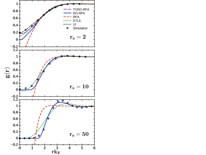
Figure 1: Spin-averaged pair correlation function $g(r)$ as a function of distance $r$ for various densities. The meanings of the curves and symbols are shown in the figure legend. For $r_{s}=$ 2 and 10, the simulation data are from Ceperley and AlderCeperley and Alder (1980) as obtained from Gori-Giorgi et al.Gori-Giorgi et al. (2000) For $r_{s}=50$, the simulation data are from Zong et al.Zong et al. (2002) The contact value $g(0)$ from the RPA theory is -0.66, -3.95 and -15.1 for $r_{s}=$ 2, 10 and 50, respectively.

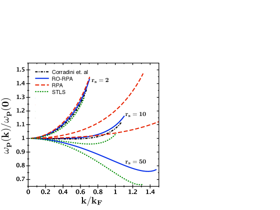
Figure 2: Plasmon dispersion curves for various scaled average electron separations $r_{s}$. The meanings of the curves are shown in the figure legend. An $r_{s}$ label refers to the closest RO-RPA curve. For the other theories, the trend is for the slope of $\omega_{p}(k)$ at small $k$ to decrease as $r_{s}$ increases. The complete RPA curve for $r_{s}=50$ is not shown, it terminating with value $\omega_{p}(k)/\omega_{p}(0)=1.55$ at $k/k_{F}=2.36$. The Corradini et al. curves were obtained using their fitCorradini et al. (1998) of $G_{+}(k,0)$ to simulation dataMoroni et al. (1995).

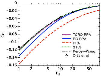
Figure 3: Scaled correlation energy per particle $\epsilon_{c}$ (in Rydbergs) as a function of the scaled average electron separation $r_{s}$. The meanings of the curves and symbols are shown in the figure legend. The Perdew-Wang curve is a fit Perdew and Wang (1992) to simulation data Ceperley and Alder (1980).

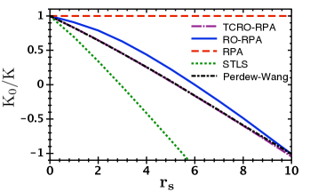
Figure 4: Scaled inverse compressibility $K_{0}/K$ as a function of the scaled average electron separation $r_{s}$, obtained using Eq.(II.3). The meanings of the curves are shown in the figure legend. Note that the TCRO-RPA and Perdew-Wang curves overlap for almost all densities shown.

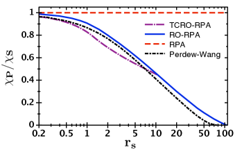
Figure 5: Scaled inverse spin susceptibility $\chi_{P}/\chi_{S}$ as a function of the scaled average electron separation $r_{s}$, obtained using Eq.(II.4). The meanings of the curves are shown in the figure legend.

As mentioned above, the focus on static properties partly justified ignoring the frequency dependence of the optimized potentials, $u_{ij}$. However, the structure of the multi-component theory is such that when mapped to the one-component form for $\chi(k,\omega)$, Eq.(II.9), the local field factor $G_{+}$ that arises is frequency dependent. It is interesting then to examine theoretical predictions for a dynamic property of the gas: its collective excitations, i.e., plasmons.Fetter and Walecka (2003); Giuliani and Vignale (2005)

Figure 2 shows the plasmon frequency $\omega_{p}$ as a function of wavevector $k$ for various theories and simulation data for the same densities as given in Figure 1. As shown, the plasmon frequency is normalized by its value at zero wavenumber: $\omega_{p}(0)=\sqrt{4\pi ne^{2}/m}$. The curves terminate at the beginning of the electron-hole continuum of the non-interacting electron gas.Giuliani and Vignale (2005) The Corradini et al. curves were obtained using their fitCorradini et al. (1998); Giuliani and Vignale (2005) of $G_{+}(k,0)$ to QMC simulation data of Moroni et al.Moroni et al. (1995) for $r_{s}=2$, 5 and 10. While not shown in the figure, the predictions of the theory of UIUtsumi and Ichimaru (1980) for $r_{s}=2$ are essentially the same as those shown for Corradini et al. As can be seen, the RO-RPA predicts larger plasmon frequencies than the STLS theory for all densities, with the difference increasing somewhat as $r_{s}$ increases. The RO-RPA predictions agree well with the results using the Corradini et al. fit for both densities, $r_{s}=2$ and 10. It has been shown elsewhere that the fully self-consistent GWA gives poor predictions for the spectral properties of jellium, including the plasmon modes.Holm and von Barth (1998)

Figure 3 shows theoretical predictions for the scaled correlation energy per particle, $\epsilon_{c}$, as a function of the scaled average electron separation, $r_{s}$. Also shown are simulation data of Ortiz et al.Ortiz et al. (1999), and the Perdew-Wang fitPerdew and Wang (1992) to simulation data of Ceperley and AlderCeperley and Alder (1980). Vosko et al.Vosko et al. (1980) show results for $\epsilon_{c}$ for other theories for the paramagnetic phase. As can be seen, the predictions of the RO-RPA greatly improve upon those of the RPA. As mentioned above, the density range of most metals is $2\leq r_{s}\leq 6$.Ashcroft and Mermin (1976) For this range, the RO-RPA values for $\epsilon_{c}$ are more negative than those of simulation by 15% on average, while the RPA values are more negative by 46% on average. The accuracy of the RO-RPA increases with decreasing density such that, for example, at $r_{s}=40$, its value for $\epsilon_{c}$ is within 3% of simulation. The thermodynamically consistent theory, TCRO-RPA, improves even more on the RPA: its predictions for $\epsilon_{c}$ are within 4% of simulation over the metallic density range. Interestingly, the predictions of the one-component RO-RPA theory, while being inferior to the multi-component theory for almost every other quantity, are slightly better than the multi-component for $\epsilon_{c}$ when thermodynamic consistency is enforced. The one-component TCRO-RPA theory agrees with the Perdew-Wang fit to within 3% for the metallic density range. This accuracy is the same or only slightly less than that of the most accurate theories for $\epsilon_{c}$: STLS,Singwi et al. (1968) and Vashishta and Singwi,Vashishta and Singwi (1972) which agree with simulation within 2% and 3%, respectively, over this density range (the UI theory agrees within 7%Utsumi and Ichimaru (1980)). While it has been tested to date for only a few densities, the fully self-consistent GWA gives very good agreement for $\epsilon_{c}$, within 1% for $r_{s}=2$ and 4.Holm and von Barth (1998) Given the mediocre predictions of the theory for other properties, this good agreement is thought to be to due to a large cancellation of effects.Holm and von Barth (2004)

Figure 4 shows results for the scaled inverse of the compressibility, $K_{0}/K$, as defined by the structure equation, Eq.(II.3) above. Simulation values were obtained using the Perdew-Wang fitPerdew and Wang (1992) to data of Ceperley and AlderCeperley and Alder (1980) for the correlation energy, and an expression relating the compressibility to the total energyGiuliani and Vignale (2005). For jellium, simulation studiesCeperley and Alder (1980) show that the inverse compressibility goes to zero at $r_{s}=5.25$. The RO-RPA predicts a zero at $r_{s}=6$, which is $14\%$ higher. As a comparison, the STLS theory predicts a zero at $r_{s}=3$, which is 55% less than simulation. As is well known, the RPA gives the non-interacting value at all densities. Interestingly, the TCRO-RPA predictions agree very well with the Perdew-Wang fitted data, within 0.1%, up to $r_{s}=8$.

Figure 5 shows results for the scaled inverse of the spin susceptibility, $\chi_{P}/\chi_{S}$, as defined by the structure equation, Eq.(II.4) above. As for $K$, simulation values were obtained using the Perdew-Wang fitPerdew and Wang (1992) for the correlation energy, and an expression relating $\chi_{S}$ to the total energyGiuliani and Vignale (2005). A divergence in $\chi_{S}$ is identified with a second-order transition from the paramagnetic state to a polarized state. In Hartree-Fock theory, this polarized state was identified with the fully polarized, i.e., ferromagnetic, state.Fetter and Walecka (2003) Simulation work appeared to have reinforced this idea.Ceperley and Alder (1980) In the Hartree-Fock and RPA theories, the density of the divergence of $\chi_{S}$ is slightly lower (higher $r_{s}$) than the density for paramagnetic-ferromagnetic phase coexistence. In their fit then, Perdew and Wang reasoned that the true density of divergence occurs at an $r_{s}$ slightly above that for paramagnetic-ferromagnetic coexistence, $r_{s}=73$, which was computed via simulation by Ceperley and Alder.Ceperley and Alder (1980) This reasoning yielded a divergence of $\chi_{S}$ at $r_{s}=77.5$. This zero of $1/\chi_{S}$ can be seen in Figure 5.

Subsequent simulation work by Ortiz et al. found that partially polarized states were energetically favorable at higher densities (lower $r_{s}$), and the transition from the paramagnetic to a partially polarized state was continuous.Ortiz et al. (1999) Later simulation work by Zong et al. underscored this picture, though their estimate of the density of this transition was lower, $r_{s}\approx 50$.Zong et al. (2002) In addition, Zong et al. estimated the transition to the ferromagnetic state was at $r_{s}\approx 100$, which was also their estimate for the transition to the Wigner solid state.Zong et al. (2002)

As can be seen in Figure 5, the RO-RPA predicts a divergence at $r_{s}\approx 107$, in good agreement with the estimate of Zong et al. for the paramagnetic-ferromagnetic transition. So, either the RO-RPA overestimates the value of $r_{s}$ for the paramagnetic-partially polarized transition by a factor of two, or predicts that only the paramagnetic-ferromagnetic transition is second order. Given the accuracy of the RO-RPA for the correlation energy at low density, the latter explanation appears more plausible. However, the RO-RPA value for the density of divergence was obtained from the structure route expression for the susceptibility, and usually estimates using the energy route are more accurate. Given the from of the RO-RPA multi-component theory, it is straightforward to generalize it to compute $E_{corr}$ as a function of the fractional spin polarization, $p\equiv\langle n_{\uparrow}(x)-n_{\downarrow}(x)\rangle/n$, and thus determine coexistence and spinodal boundaries. The solution to this puzzle then is left to future research.

In this work, thermodynamic consistency was enforced on the compressibility, which is a measure of the sensitivity of the electron density to changes in the pressure. It is not expected then that this method would necessarily improve the predictions of the theory for the spin susceptibility, which is a measure of the sensitivity of a different quantity, the spin polarization, to changes in the magnetic field. Nonetheless, it is interesting to examine the TCRO-RPA predictions for $\chi_{S}$. As can be seen in Figure 5, the TCRO-RPA values agree well with the Perdew-Wang fit at very high density (small $r_{s}$), but drop below the Perdew-Wang curve at $r_{s}\approx 0.5$. For example, at $r_{s}=2$, the TCRO-RPA value is 10% below the Perdew-Wang one. For $r_{s}>2$, the TCRO-RPA curve asymptotically approaches the RO-RPA curve, terminating at it at $r_{s}\approx 10.8$. At that point, the TCRO-RPA curve is above the Perdew-Wang curve. In other words, the agreement with the fitted simulation data appears to be better for the RO-RPA than for the TCRO-RPA. It has been remarked elsewhere that the Perdew-Wang fit is not that accurate for polarized states.Giuliani and Vignale (2005) It seems unlikely though that this inaccuracy would be that large near $p=0$. A clarifying task then would be to compute $\chi_{S}$ via the energy route. For this, $E_{corr}$ would be computed for small $p$ and constant $r_{s}$, while enforcing thermodynamic consistency on $K$ (or even $\chi_{S}$).

V Summary and discussion

In summary, the range optimization scheme was applied to the RPA theory for jellium. It was shown that this RO-RPA theory gives greatly improved predictions for the gas properties as shown by its results for the pair correlation function $g(r)$, compressibility $K$ and spin susceptibility $\chi_{S}$. For the correlation energy, $E_{corr}$, the theory is most accurate at low densities, but it still gives predictions within 15% of simulation for the density range of most metals, $2\leq r_{s}\leq 6$. Enforcing thermodynamic consistency on the compressibility improves the agreement with simulation to within 4% for this density range, while the one-component version of the theory is slightly better at 3%. This agreement is comparable to the most accurate of the previous theories for $E_{corr}$.Singwi et al. (1968); Vashishta and Singwi (1972); Holm and von Barth (1998) Also, the RO-RPA appears to outperform the STLS theory in comparison with simulation data for the plasmon modes and compressibility, and the pair correlation function at low density.

The thermodynamically consistent theory could be further improved by conducting the range optimization to obey the cusp condition on $g(r)$ near $r=0$.Kimball (1973) Also, since range optimization can be applied to any theory in which the positivity condition of $g(r)$ is violated, improvements in the accuracy of the basic theory are possible.

One noteworthy result was that the RO-RPA theory predicts a divergence of $\chi_{S}$ at a density that is lower than current estimates for the liquid-solid transition.Zong et al. (2002); Giuliani and Vignale (2005) Thus, no divergence of $\chi_{S}$ is predicted for the liquid phase. This result was obtained using the structure route expression for $\chi_{S}$, Eq.(II.4). Given the evidence from simulations for a transition to partially polarized states,Ortiz et al. (1999); Zong et al. (2002) it would be interesting within the RO-RPA to examine the phase behavior of jellium as a function of polarization using the energy route.Tanaka and Ichimaru (1989) Further, since the temperature dependent density-density response function can be represented by an equation almost identical to Eq.(II.7),Fetter and Walecka (2003) the full temperature dependent phase diagram can be obtained.

As stated above, one aim of this work is to apply range optimization to inhomogeneous electron liquids, to compute the band structure of semiconductors, for example. It was shown in Sec.III how the new algorithm to implement range optimization can be applied to inhomogeneous liquids, and results for that will be presented in a future work.