Rescattering effects in laser-assisted electron-atom bremsstrahlung

Abstract

Rescattering effects in nonresonant spontaneous laser-assisted electron-atom bremsstrahlung (LABrS) are analyzed within the framework of time-dependent effective-range (TDER) theory. It is shown that high energy LABrS spectra exhibit rescattering plateau structures that are similar to those that are well-known in strong field laser-induced processes as well as those that have been predicted theoretically in laser-assisted collision processes. In the limit of a low-frequency laser field, an analytic description of LABrS is obtained from a rigorous quantum analysis of the exact TDER results for the LABrS amplitude. This amplitude is represented as a sum of factorized terms involving three factors, each having a clear physical meaning. The first two factors are the exact field-free amplitudes for electron-atom bremsstrahlung and for electron-atom scattering, and the third factor describes free electron motion in the laser field along a closed trajectory between the first (scattering) and second (rescattering) collision events. Finally, a generalization of these TDER results to the case of LABrS in a Coulomb field is discussed.

1 Introduction

An intense laser field significantly modifies the bremsstrahlung (BrS) process accompanying electron-atom or electron-ion scattering, i.e., an electron colliding with a target can efficiently convert the combined energies of a number of laser photons, each with energy $\hbar\omega$, into the energy of a spontaneously emitted photon $\hbar\Omega$. In comparison with field-free BrS, in laser-assisted BrS (LABrS) the spectral energies can be significantly extended and resonant-like enhancements of the LABrS cross sections may appear.

There have been relatively few prior studies of LABrS processes. Karapetyan and Fedorov [1] have shown that LABrS spectra for electron scattering from a Coulomb potential exhibit resonant peaks (at $\Omega=k\omega$, where $k$ is integer), which occur only in the limit of an intense laser field. The electron-Coulomb interaction was treated in [1] within the Born approximation. Zhou and Rosenberg [2] investigated LABrS beyond the Born approximation in the scattering potential for the case of a low-frequency laser field. They found a series of resonant peaks in the BrS spectrum, separated by $\hbar\omega$, that are related to resonant features in field-free electron-atom scattering. The approach used in [2] is based on the low-frequency Kroll-Watson result [3] for the electron scattering state and its “resonant” modification. These two seminal works by Karapetyan and Fedorov [1] and by Zhou and Rosenberg [2] have led to a number of more recent analyses. These have been described briefly in section 4.5 of the review of Ehlotzky et al. [4]. A comparative analysis of LABrS for electron-Coulomb scattering within the Born and low-frequency approximations (in accordance with [1] and [2] respectively) has been given in a recent paper by Dondera and Florescu [5], who also review there other works on non-relativistic LABrS.

A common feature of the above works is that they do not describe effects of laser-induced electron rescattering on an atomic target. These rescattering effects are well known in multiphoton processes involving bound atomic states, such as high-order harmonic generation (HHG) and above-threshold ionization/detachment (ATI/ATD). In those processes they lead to the appearance of broad, plateau-like structures in the HHG and ATI/ATD spectra [6, 7, 8]. Also, plateaus in the high-energy (multiphoton) spectra of laser-assisted collisional processes involving an initially free (i.e., continuum) electron have been predicted for laser-assisted electron scattering (LAES) [9, 10] and laser-assisted radiative recombination/attachment (LARR/LARA) [11, 12]. Interest in such plateaus centers on the possibility of transferring large amounts of energy from a laser field into either electron kinetic energy or high-energy spontaneous photons (or harmonics) without significant decreases in the yields as the number $n$ of absorbed photons increases over a wide interval of $n$.

The theoretical description of laser-assisted electron-atom processes for the case of an intense laser field necessarily requires an accurate treatment of both the electron-laser and electron-atom interactions in order to properly describe the strong field plateau phenomena. An appropriate approach that meets this requirement is based on time-dependent effective range (TDER) theory [13], which combines the effective range theory (for the electron-atom interaction) with the quasienergy or Floquet theory (for the electron-laser field interaction). This approach was employed recently to describe resonant phenomena in the LABrS process [14]. Namely, a resonant mechanism for LABrS involving the resonant transition into a laser-dressed intermediate quasi-bound state (corresponding respectively to a field-free bound state of either a neutral atom or a negative ion) accompanied by ionization or detachment of this state by the laser field has been considered. However, rescattering effects were not investigated in [14]. An important advantage of the TDER theory is that it allows an accurate quantum derivation of closed-form analytic formulas for the cross sections of strong field processes that take into account the rescattering effects non-perturbatively in the limit of a low frequency laser field. Such formulas were obtained for both laser-induced processes ( such as HHG [15] and ATI/ATD [16]) and laser-assisted collisional processes (such as LAES [17, 18] and LARR/LARA [12]). For collisional processes, the analytic formulas describe accurately the high-energy part of the electron (for LAES) or photon (for LARR/LARA) spectra, which cannot be described using the well-known Bunkin-Fedorov [19] or Kroll-Watson [3] approximations. The analytic results have a factorized structure, in which the atomic factors represent exact field-free amplitudes evaluated using the instantaneous kinetic electron momenta in the laser field, thus allowing us to generalize the effective range approximation to the case of an arbitrary atomic potential.

In this paper, we consider rescattering effects in nonresonant LABrS, i.e., we study the process of spontaneous photon emission during electron-atom scattering for electron energies and laser field parameters such that resonant radiative (spontaneous or stimulated) transitions into an intermediate quasi-bound state are negligible and thus are not taken into account. In the low-frequency approximation, we derive an analytic description of the rescattering plateau features in LABrS spectra and analyze numerically the accuracy of the derived analytic formulas. These analytic results permit a transparent physical interpretation and present the first quantum justification of the three-step rescattering scenario for the description of radiative (with emission of a spontaneous photon) continuum-continuum transitions of an electron interacting with both an atomic potential and an intense laser field.

This paper is organized as follows. In section 2 we present results for the LABrS amplitude in terms of the exact TDER expressions for initial and final states of the scattered electron. In section 3 we present an analysis of the LABrS amplitude in the limit of low frequencies. We start in section 3.1 with the low-frequency expansion of the most important ingredient determining a TDER scattering state. In section 3.2 we present the low-frequency result for the amplitude for “direct” LABrS, i.e., neglecting rescattering. Basic results (47) – (49) for the “rescattering” part, $\mathbf{d}^{{(\mathrm{rsc})}}_{n}$, of the LABrS amplitude are obtained in section 3.3 using the regular saddle point method. Based on results of section 3.3, in section 3.4 we discuss the three-step rescattering scenario for the LABrS process and its relation to the corresponding scenario for LAES. In section 3.5 we consider the case of two merging saddle points, which requires the use of special saddle point methods in order to estimate the contributions of coalescing electron trajectories to the rescattering amplitude $\mathbf{d}^{{(\mathrm{rsc})}}_{n}$. Our numerical results and discussions are presented in section 4. In section 4.1 we demonstrate good agreement between exact TDER results and those obtained in the low-frequency approximation for the high-energy rescattering plateau part of LABrS spectra. We discuss there also some peculiarities in LABrS spectra (such as their oscillation patterns and interference enhancements). In section 4.2 we generalize our TDER results, which are valid for a short-range atomic potential, to the case of LABrS in a Coulomb potential and present numerical estimates for electron-proton LABrS. In section 5 we present our conclusions. In the Appendix we present some mathematical details.

2 General results for LABrS within TDER theory

We consider the LABrS process for the case of a linearly polarized monochromatic laser field described by the electric field vector ${\bf F}(t)$,

$$\mathbf{F}(t)=\mathbf{e}_{z}F\cos\omega t,$$ (1)

where $F$ is the field amplitude and $\mathbf{e}_{z}$ is the unit polarization vector. For the electron-laser interaction, we use the dipole approximation in the length gauge $V(\mathbf{r},t)=-e\mathbf{r}\cdot\mathbf{F}(t)$. To describe electron-atom collisions in a time-periodic field (1), the quasienergy (or Floquet) approach is most appropriate. Within this approach, the laser-dressed scattering state of an electron with asymptotic momentum $\mathbf{p}$ and kinetic energy $E=p^{2}/(2m)$ has the form (cf., e.g., [20]):

$$\Psi_{\mathbf{p}}(\mathbf{r},t)=\Phi_{\mathbf{p}}(\mathbf{r},t)e^{-i\epsilon t/\hbar},$$

$$\Phi_{\mathbf{p}}(\mathbf{r},t)=\Phi_{\mathbf{p}}(\mathbf{r},t+T),\quad T=2\pi/\omega,$$ (2)

where $\epsilon$ is the quasienergy, $\epsilon=E+u_{p}$, and $u_{p}=e^{2}F^{2}/(4m\omega^{2})$ is the ponderomotive (or quiver) energy of an electron in the laser field (1).

For given initial ($\mathbf{p}_{i}$) and final ($\mathbf{p}_{f}$) electron momenta, the LABrS process consists in the spontaneous emission of a photon with energy $\hbar\Omega=(p_{i}^{2}-p_{f}^{2})/(2m)+n\hbar\omega$ (where $n$ is the number of absorbed, $n>0$, or emitted, $n<0$, laser photons) and polarization vector ${\bf e}^{\prime}$ $({\bf e}^{\prime}\cdot{\bf e}^{\prime*}=1)$. The amplitude for this process is proportional to the scalar product $\mathbf{e}^{\prime*}\cdot\mathbf{d}_{n}$ of the polarization vector and the Fourier component $\mathbf{d}_{n}\equiv\mathbf{d}_{n}(\mathbf{p}_{i},\mathbf{p}_{f})$ of the dipole matrix element $\langle\Phi_{\mathbf{p}_{f}}^{{\cal{T}}}|\mathbf{d}|\Phi_{\mathbf{p}_{i}}\rangle$,

$$\mathbf{d}_{n}=\frac{1}{T}\int\limits_{0}^{T}dte^{in\omega t}\langle\Phi_{\mathbf{p}_{f}}^{{\cal{T}}}(t)|\mathbf{d}|\Phi_{\mathbf{p}_{i}}(t)\rangle,\quad\mathbf{d}=e\mathbf{r},$$ (3)

where $\Phi_{\mathbf{p}}(t)\equiv\Phi_{\mathbf{p}}(\mathbf{r},t)$ and $\Phi_{\mathbf{p}}^{{\cal{T}}}(\mathbf{r},t)$ [$=\Phi_{-\mathbf{p}}^{*}(\mathbf{r},-t)$] is the corresponding time-reversed wave function [14]. The LABrS doubly differential cross section with respect to the emitted photon frequency $\Omega$ and the final electron direction (into the solid angle element $d\Omega_{{\bf p}_{f}}$), summed over polarizations and integrated over the directions of the emitted photon, has the following form:

$$\frac{d^{2}\sigma_{n}(\mathbf{p}_{i},\mathbf{p}_{f})}{d\Omega d\Omega_{\mathbf{p}_{f}}}=\frac{m^{2}\Omega^{3}}{6(\pi\hbar c)^{3}}\frac{p_{f}}{p_{i}}|\mathbf{d}_{n}(\mathbf{p}_{i},\mathbf{p}_{f})|^{2}.$$ (4)

We use the TDER theory to describe the field-dressed continuum state ($\Phi_{{\bf p}}$) of the active electron [18, 21] scattered from a short-range atomic potential $U(r)$ that vanishes for $r\gtrsim r_{c}$. The TDER theory assumes that the potential $U(r)$ supports a single weakly-bound state (a negative ion state) with energy $E_{0}=-\hbar^{2}\kappa^{2}/(2m)$ $(\kappa r_{c}\ll 1)$ and angular momentum $l$. The electron-atom interaction is described by the $l$-wave scattering phase $\delta_{l}(p)$, which is parameterized by the scattering length $a_{l}$ and the effective range $r_{l}$, which are parameters of the problem:

$$k^{2l+1}\cot\delta_{l}(p)=-a_{l}^{-1}+r_{l}k^{2}/2,\quad k=p/\hbar.$$

For simplicity, in this paper we consider the case of a bound $s$-state ($l=0$), so that only the phase shift $\delta_{0}(p)$ is nonzero.

The scattering state $\Phi_{{\bf p}}({\bf r},t)$ may be presented as a sum of the “incident” plane wave, $\chi_{\mathbf{p}}(\mathbf{r},t)$, and the scattered “outgoing” wave, $\Phi_{\mathbf{p}}^{(+)}(\mathbf{r},t)$,

$$\Phi_{\mathbf{p}}(\mathbf{r},t)=\chi_{\mathbf{p}}(\mathbf{r},t)+\Phi_{\mathbf{p}}^{(+)}(\mathbf{r},t).$$ (5)

The function $\chi_{\mathbf{p}}$ is the time-periodic part of the wave function of a free electron with momentum $\mathbf{p}$ in the laser field ${\bf F}(t)$ (the Volkov wave function),

$$\chi_{\mathbf{p}}(\mathbf{r},t)=e^{i[\mathbf{P}(t)\cdot\mathbf{r}+S_{\mathbf{p}}(t)]/\hbar},$$

$$S_{\mathbf{p}}(t)=-\int^{t}[\mathbf{P}^{2}(\tau)/(2m)-\epsilon]d\tau$$

$$=\frac{eF\mathbf{e}_{z}\cdot\mathbf{p}}{m\omega^{2}}\cos\omega t+\frac{u_{p}}{2\omega}\sin 2\omega t,$$ (6)

where $\mathbf{P}(t)=\mathbf{p}-(e/c)\mathbf{A}(t)$ is the electron’s kinetic momentum in the laser field, while $\mathbf{A}(t)=-(\mathbf{e}_{z}Fc/\omega)\sin\omega t$ is the vector potential of the laser field.

Within the TDER approach, the scattered electron wave function $\Phi_{\mathbf{p}}^{(+)}$ in (5) is expressed in terms of a one-dimensional integral [21], involving the retarded Volkov Green’s function, $G^{(+)}({\bf r},t;{\bf r}^{\prime},t^{\prime})$, for a free electron in the laser field ${\bf F}(t)$:

$$\Phi_{\mathbf{p}}^{(+)}(\mathbf{r},t) = -\frac{2\pi\hbar^{2}}{m}\int_{-\infty}^{t}dt^{\prime}e^{i\epsilon(t-t^{\prime})/\hbar}$$ (7)

$$\times G^{(+)}(\mathbf{r},t;0,t^{\prime})f_{\mathbf{p}}(t^{\prime}),$$

The time-inverted scattering state $\Phi_{\mathbf{p}}^{{\cal{T}}}$, involved in the transition matrix element in (3), has the form (5) with the scattered wave $\Phi_{{\bf p}}^{(+)}$ replaced by the wave function $\Phi_{{\bf p}}^{(-)}$: $\Phi_{\mathbf{p}}^{{\cal{T}}}=\chi_{{\bf p}}+\Phi_{{\bf p}}^{(-)}$. The function $\Phi_{{\bf p}}^{(-)}$ has the asymptotic form of an “ingoing” wave and is expressed in terms of the advanced Volkov Green’s function, $G^{(-)}$:

$$\Phi_{\mathbf{p}}^{(-)}(\mathbf{r},t) = -\frac{2\pi\hbar^{2}}{m}\int_{t}^{\infty}dt^{\prime}e^{i\epsilon(t-t^{\prime})/\hbar}$$ (8)

$$\times G^{(-)}(\mathbf{r},t;0,t^{\prime})f^{*}_{-\mathbf{p}}(-t^{\prime}).$$

For the Volkov Green’s functions, $G^{(\pm)}$, we use the well-known Feynman form:

$$G^{(\pm)}({\bf r},t;{\bf r}^{\prime},t^{\prime}) = \mp\theta[\pm(t-t^{\prime})]\frac{i}{\hbar}\left[\frac{m}{2\pi i\hbar(t-t^{\prime})}\right]^{3/2}$$ (9)

$$\times \exp[iS({\bf r},t;{\bf r}^{\prime},t^{\prime})/\hbar],$$

where $S({\bf r},t;{\bf r}^{\prime},t^{\prime})$ is the classical action of the active electron in the field $\mathbf{F}(t)$ (cf., e.g., [14]). In the absence of the laser field (${\bf F}(t)=0$), the functions $\Phi_{{\bf p}}^{(\pm)}$ reduce to the wave functions $\psi_{\bf p}^{(\pm)}$ for the field-free problem of elastic electron scattering on the potential $U(r)$ having asymptotic forms of spherical outgoing (+) or ingoing (-) waves:

$$\psi_{\bf p}^{(\pm)}(r)\big{|}_{r\gg r_{c}}=\mathcal{A}(p)\frac{e^{\pm ipr/\hbar}}{r},$$

where $\mathcal{A}(p)$ is the field-free $s$-wave scattering amplitude in the effective range approximation:

$$\mathcal{A}(p)=\frac{1}{-a_{0}^{-1}-ip/\hbar+r_{0}p^{2}/(2\hbar^{2}).}$$ (10)

The time-periodic function $f_{\bf p}(t)=\sum_{k}f_{k}({\bf p})e^{-ik\omega t}$ appearing in the wave functions (7) and (8) is the key object of TDER theory. It contains the entire information about the details of the electron-atom dynamics in the laser field and enters into the expressions for the amplitudes of laser-assisted collisions (cf., e.g., the results in [21] for the LAES amplitude). The function $f_{{\bf p}}(t)$ satisfies an inhomogeneous integro-differential equation (cf. equation (23) in [18]), which can be converted to a system of inhomogeneous linear equations for its Fourier coefficients $f_{k}({\bf p})$ (cf. Appendix A in [18]).

The TDER result for the LABrS dipole moment $\mathbf{d}_{n}$ [given by expression (3)] follows after substituting the wave functions of the initial ($\Phi_{{\bf p}_{i}}$) and final ($\Phi_{{\bf p}_{f}}$) scattering states in the form (5) [taking into account (7) and (8)] into equation (3) (for details of the derivation, see [14]):

$$\mathbf{d}_{n}=\mathbf{d}^{(TS)}_{n}+{\hat{\mathbf{d}}}_{n}+{\tilde{\mathbf{d}}_{n}}.$$ (11)

In the result (11), the term $\mathbf{d}^{(TS)}_{n}$ corresponds to the Thomson scattering (TS) of the laser radiation from a free electron,

$$\mathbf{d}_{n}^{(TS)}=\frac{1}{T}\int\limits_{0}^{T}dt\,e^{in\omega t}\langle\chi_{\mathbf{p}_{f}}(t)|\mathbf{d}|\chi_{\mathbf{p}_{i}}(t)\rangle,$$

and is nonzero only for $\Omega=\omega$ $(n=1)$. In what follows, we omit this term from our considerations. Other terms in expression (11) are given by the following matrix elements:

$${\hat{\mathbf{d}}}_{n}=\frac{1}{T}\int\limits_{0}^{T}dte^{in\omega t}\Big{(}\langle\chi_{\mathbf{p}_{f}}(t)|\mathbf{d}|\Phi_{\mathbf{p}_{i}}^{(+)}(t)\rangle$$

$$\phantom{{{\hat{\mathbf{d}}}_{n}}}+\langle\Phi_{\mathbf{p}_{f}}^{(-)}(t)|\mathbf{d}|\chi_{\mathbf{p}_{i}}(t)\rangle\Big{)},$$ (12)

$${\tilde{\mathbf{d}}_{n}}=\frac{1}{T}\int\limits_{0}^{T}dte^{in\omega t}\langle\Phi_{\mathbf{p}_{f}}^{(-)}(t)|\mathbf{d}|\Phi_{\mathbf{p}_{i}}^{(+)}(t)\rangle.$$ (13)

The derivation of the final results for the dipole matrix elements (12) and (13) without using any approximations for the TDER scattering states $\Phi_{\mathbf{p}_{i}}^{(+)}$ and $\Phi_{\mathbf{p}_{f}}^{(-)}$ can be found in [14]. These exact TDER results for the LABrS amplitude are complicated since they contain infinite series involving Fourier coefficients of the functions $f_{\mathbf{p}_{i}}(t)$ and $f_{-\mathbf{p}_{f}}(-t)$, which can be obtained only numerically. For a non-perturbative analytic analysis of rescattering effects, we shall thus employ the low-frequency approximation.

3 Low-frequency analysis of the LABrS amplitude

3.1 Low-frequency results for $f_{{\bf p}}(t)$

In a low-frequency laser field (such that the condition $\hbar\omega\ll u_{p}$ is fulfilled), the equation for $f_{\bf p}(t)$ can be solved analytically using an iterative approach for taking into account the rescattering effects. This iterative approach has been developed in [18]. As a result, the function $f_{\bf p}(t)$ can be presented as a sum of two terms,

$$f_{\mathbf{p}}(t)=f^{{(\mathrm{dr})}}_{\mathbf{p}}(t)+f^{{(\mathrm{rsc})}}_{\mathbf{p}}(t),$$ (14)

where the first term corresponds to the Kroll-Watson approximation for the scattering state [17, 18]:

$$f^{{(\mathrm{dr})}}_{\mathbf{p}}(t)=\mathcal{A}[P(t)]e^{iS_{\mathbf{p}}(t)/\hbar},$$ (15)

which describes the “direct” (without rescattering) LAES. The second term in (14) represents the first-order “rescattering” correction to the zero-order result (15). It involves the product of two field-free electron-atom scattering amplitudes with laser-modified instantaneous momenta, thus describing electron-atom rescattering (cf. [18]):

$$f^{{(\mathrm{rsc})}}_{\mathbf{p}}(t)=\sum_{k}\mathcal{A}\left[Q(t,t^{\prime}_{k})\right]\chi_{\mathbf{p}}(t,t^{\prime}_{k}),$$ (16)

$$\chi_{\mathbf{p}}(t,t^{\prime}_{k})=\frac{\mathcal{A}\left[P(t^{\prime}_{k})\right]e^{i\varphi_{\mathbf{p}}(t,t^{\prime}_{k})}}{\sqrt{(\hbar/m)(t-t^{\prime}_{k})^{3}\mathcal{D}_{\mathbf{p}}(t,t^{\prime}_{k})}},$$ (17)

where

$$\mathbf{Q}(t,t^{\prime})=\mathbf{q}(t,t^{\prime})-\frac{e}{c}\mathbf{A}(t),$$ (18)

$$\mathbf{q}(t,t^{\prime})=\frac{e}{\omega^{2}}\frac{\mathbf{F}(t)-\mathbf{F}(t^{\prime})}{t-t^{\prime}},$$ (19)

$$\varphi_{\mathbf{p}}(t,t^{\prime})=\left[\epsilon(t-t^{\prime})+S(t,t^{\prime})+S_{\mathbf{p}}(t^{\prime})\right]/\hbar$$

$$=\frac{(t-t^{\prime})(\mathbf{p}-\mathbf{q}(t,t^{\prime}))^{2}}{2m\hbar}+\frac{S_{\mathbf{p}}(t)}{\hbar},$$ (20)

$$\mathcal{D}_{\mathbf{p}}(t,t^{\prime})=\partial^{2}\varphi_{\mathbf{p}}(t,t^{\prime})/\partial t^{\prime 2}$$

$$=\frac{\mathbf{Q}^{2}(t^{\prime},t)}{m\hbar(t-t^{\prime})}+\frac{e\mathbf{F}(t^{\prime})\cdot(\mathbf{q}(t,t^{\prime})-\mathbf{p})}{m\hbar},$$ (21)

where $S(t,t^{\prime})\equiv S(0,t;0,t^{\prime})$. For $\mathbf{Q}(t,t^{\prime})$ in (18) we have the following relation:

$$\mathbf{Q}(t^{\prime},t)=\mathbf{Q}(t,t^{\prime})+\frac{e}{c}\mathbf{A}(t)-\frac{e}{c}\mathbf{A}(t^{\prime}).$$

The summation in (16) is taken over the saddle points $t^{\prime}_{k}$ of the phase function $\varphi_{\bf p}(t,t^{\prime})$ given by equation (20). These saddle points satisfy the equation $(\partial\varphi_{\mathbf{p}}(t,t^{\prime})/\partial t^{\prime})|_{t^{\prime}=t^{\prime}_{k}}=0$ or, explicitly,

$$\mathbf{P}^{2}(t^{\prime}_{k})=\mathbf{Q}^{2}(t^{\prime}_{k},t).$$ (22)

The equation (22) has a clear physical meaning: it represents the energy conservation law for the electron scattering event at the time $t^{\prime}_{k}$ with exchange of the kinetic momentum from $\mathbf{P}(t^{\prime}_{k})$ to the “intermediate” laser-induced momentum $\mathbf{Q}(t^{\prime}_{k},t)$. This latter momentum ensures the condition for the electron return by the laser field back to the atom at the time moment $t$, followed by the recollision. We note that the saddle points $t_{k}^{\prime}$ are functions of the time $t$ ($t_{k}^{\prime}\equiv t_{k}^{\prime}(t)$) implicitly defined by equation (22).

The results (15) and (16) are not applicable for resonant electron energies, $E\approx\mu\hbar\omega+E_{0}-u_{p}$, at which the electron may be temporarily captured in a bound state of the atomic potential by emitting $\mu$ photons [22]. Nor are they applicable for threshold energies, $E=\nu\hbar\omega,$ $\nu=1,2,\ldots$, at which the function $f_{\mathbf{p}}(t)$ may be affected considerably by threshold phenomena, corresponding to the closing (or opening) of the channel for stimulated emission of $\nu$ laser photons by the incident electron [21]. Thus, in this paper we consider the LABrS process only for non-resonant and non-threshold conditions.

3.2 Low-frequency result for the “direct” LABrS amplitude $\mathbf{d}^{{(\mathrm{dr})}}_{n}$

Using the “rescattering” expansion (14) for the function $f_{\bf p}(t)$, which determines the wave functions $\Phi_{\mathbf{p}_{i}}^{(+)}({\bf r},t)$ and $\Phi_{\mathbf{p}_{f}}^{(-)}({\bf r},t)$, we can build the “rescattering” expansion for the LABrS dipole moment $\mathbf{d}_{n}$, representing it in the form:

$$\mathbf{d}_{n}=\mathbf{d}^{{(\mathrm{dr})}}_{n}+\mathbf{d}^{{(\mathrm{rsc})}}_{n},$$ (23)

where the term $\mathbf{d}^{{(\mathrm{dr})}}_{n}$ corresponds to the “direct” LABrS process, while the term $\mathbf{d}^{{(\mathrm{rsc})}}_{n}$ (the first order “rescattering” correction to $\mathbf{d}^{{(\mathrm{dr})}}_{n}$) describes the rescattering effects in the LABrS amplitude. The “direct” term $\mathbf{d}^{{(\mathrm{dr})}}_{n}$ may be obtained from the dipole moment ${\hat{\mathbf{d}}}_{n}$ given by expression (12). The matrix element in equation (13) for ${\tilde{\mathbf{d}}_{n}}$ contains the product of two functions, $f_{{\bf p}_{i}}(t)$ and $f_{-{\bf p}_{f}}(-t)$ [cf. (7) and (8)], each of them being proportional to the field-free electron-atom scattering amplitude, which means that ${\tilde{\mathbf{d}}_{n}}$ describes rescattering effects in LABrS and should thus be neglected when calculating the zero-order term $\mathbf{d}^{{(\mathrm{dr})}}_{n}$.

Let us analyze first the dipole moment ${\hat{\mathbf{d}}}_{n}$. It has the following explicit form (cf. [14]):

$${\hat{\mathbf{d}}}_{n}=\frac{\pi\hbar e^{2}F}{m^{2}\Omega^{2}\omega}\Bigg{[}\frac{2i\omega}{eF}\left(\mathbf{p}_{i}\mathcal{L}^{(1)}_{n}-\mathbf{p}_{f}\mathcal{L}^{(2)}_{n}\right)$$

$$+\mathbf{e}_{z}\sum_{s=\pm 1}\frac{\mathcal{L}^{(1)}_{n+s}-\mathcal{L}^{(2)}_{n+s}}{\omega/\Omega+s}\Bigg{]},$$

where

$$\mathcal{L}_{n}^{(1,2)}=\frac{1}{T}\int_{0}^{T}dte^{in\omega t}L^{(1,2)}(t),$$ (24)

where

$$L^{(1)}(t)=f_{-{\bf p}_{f}}(-t)e^{iS_{{\bf p}_{i}}(t)/\hbar},$$ (25)

$$L^{(2)}(t)=f_{{\bf p}_{i}}(t)e^{iS_{-{\bf p}_{f}}(-t)/\hbar}.$$ (26)

We restrict our considerations to the high-energy LABrS spectrum, in which the emitted photon energy is much greater than the laser photon energy,

$$\hbar\Omega\gg\hbar\omega.$$ (27)

Assuming (27) and taking into account (3.2), we obtain for the dipole moment ${{\hat{\mathbf{d}}}_{n}}$:

$${{\hat{\mathbf{d}}}_{n}}=\frac{2\pi ie\hbar}{m^{2}\Omega^{2}}\frac{1}{T}\int_{0}^{T}dte^{in\omega t}$$

$$\times\Big{[}L^{(1)}(t)\mathbf{P}_{i}(t)-L^{(2)}(t)\mathbf{P}_{f}(t)\Big{]},$$ (28)

where $\mathbf{P}_{i,f}(t)=\mathbf{p}_{i,f}-(e/c)\mathbf{A}(t)$.

The result for the zero-order approximation $\mathbf{d}^{{(\mathrm{dr})}}_{n}$ follows from (28) in three steps: (1) we substitute the zero-order approximation $f_{\bf p}^{{(\mathrm{dr})}}(t)$ [given by (15)] for $f_{\bf p}(t)$ into the results (25) and (26) for $L^{(1,2)}(t)$; (2) we substitute the results obtained for $L^{(1,2)}(t)$ into (28); (3) the integral over time in (28) is evaluated using the saddle point method. As a result, for $\mathbf{d}^{{(\mathrm{dr})}}_{n}$ we obtain (cf. [14]):

$$\mathbf{d}_{n}^{{(\mathrm{dr})}}(\mathbf{p}_{i},\mathbf{p}_{f})=i^{n}J_{n}(\rho)\,\mathbf{d}^{(0)}\left[\mathbf{P}_{i}(t_{0}),\mathbf{P}_{f}(t_{0})\right],$$ (29)

where $\mathbf{d}^{(0)}$ is the field-free BrS dipole moment in the effective range approximation:

$$\mathbf{d}^{(0)}(\mathbf{p},\mathbf{p}^{\prime})=\frac{8\pi ie\hbar^{3}}{(\mathbf{p}^{2}-\mathbf{p}^{\prime 2})^{2}}\big{[}\mathbf{p}\mathcal{A}(p^{\prime})-\mathbf{p}^{\prime}\mathcal{A}(p)\big{]},$$ (30)

$\rho=eF(\mathbf{p}_{i}-\mathbf{p}_{f})\cdot\mathbf{e}_{z}/(m\hbar\omega^{2})$, $J_{n}$ is a Bessel function and the saddle point $t_{0}$ satisfies the equation $\rho\sin\omega t_{0}=n$ or $\mathbf{P}_{i}^{2}(t_{0})-\mathbf{P}_{f}^{2}(t_{0})=2m\hbar\Omega$.

3.3 Saddle-point result for the “rescattering” part, $\mathbf{d}^{{(\mathrm{rsc})}}_{n}$, of the LABrS amplitude

In order to find the rescattering correction, ${{\hat{\mathbf{d}}}_{n}}^{{(\mathrm{rsc})}}$, to the result (29) originating from the dipole moment ${{\hat{\mathbf{d}}}_{n}}$, we replace the functions $f_{\mathbf{p}_{i,f}}$ in expressions (25) and (26) for $L^{(1,2)}(t)$ by their rescattering approximations $f_{\mathbf{p}_{i,f}}\approx f_{\mathbf{p}_{i,f}}^{{(\mathrm{rsc})}}$ given by (16). The result for the dipole moment ${{\hat{\mathbf{d}}}_{n}}^{{(\mathrm{rsc})}}$ then follows from (28) after substituting there the “rescattering approximations” for $L^{(1,2)}(t)$. The result can be presented in the form:

$${{\hat{\mathbf{d}}}_{n}}^{{(\mathrm{rsc})}}=\frac{1}{T}\int_{0}^{T}dt\Big{(}\sum_{k}\hat{\bm{\mathcal{D}}}+\sum_{k}\hat{\bm{\mathcal{D}}}\big{|}_{\mathcal{G}}\Big{)},$$ (31)

where

$$\hat{\bm{\mathcal{D}}}=-\frac{2\pi ie\hbar}{m^{2}\Omega^{2}}\mathbf{P}_{f}(t)\mathcal{A}\left[Q(t,t^{\prime}_{k})\right]$$

$$\times\chi_{\mathbf{p}_{i}}(t,t^{\prime}_{k})e^{in\omega t-iS_{\mathbf{p}_{f}}({t})/\hbar},$$ (32)

and the symbol $\mathcal{G}$ in (31) implies the following set of replacements in $\hat{\bm{\mathcal{D}}}$:

$$\mathcal{G}=\{\mathbf{p}_{i}\leftrightarrow-\mathbf{p}_{f},t\to-t,t^{\prime}_{k}\to-t^{\prime}_{k},n\to-n\}.$$ (33)

The first summation (over $\hat{\bm{\mathcal{D}}}$) in the integrand of (31) is taken over saddle points $t^{\prime}_{k}=t^{\prime}_{k}(t)$ that satisfy the equation:

$$\mathbf{P}_{i}^{2}(t^{\prime}_{k})=\mathbf{Q}^{2}(t^{\prime}_{k},t),\quad t^{\prime}_{k}<t.$$ (34)

The second summation in the integrand of (31) is over $\hat{\bm{\mathcal{D}}}\big{|}_{\mathcal{G}}$ , which contains $\chi_{-\mathbf{p}_{f}}(-t,-t^{\prime}_{k})$ [cf. (32) and (33)]. It involves the saddle points $t^{\prime}_{k}$ satisfying the equation:

$$\mathbf{Q}^{2}(t^{\prime}_{k},t)=\mathbf{P}_{f}^{2}(t^{\prime}_{k}),\quad t^{\prime}_{k}>t.$$ (35)

Both equations (34) and (35) follow from the saddle point equation (22).

Let us consider now the rescattering approximation for the dipole moment ${\tilde{\mathbf{d}}_{n}}$ given by (13). As shown in the Appendix, ${\tilde{\mathbf{d}}_{n}}$ can be expressed as the sum of two terms:

$${{\tilde{\mathbf{d}}_{n}}}={{\tilde{\mathbf{d}}_{n}}}^{(+)}+{{\tilde{\mathbf{d}}_{n}}}^{(-)},$$ (36)

$${{\tilde{\mathbf{d}}_{n}}}^{(+)}=\frac{e}{\Omega^{2}}\sqrt{\frac{2\pi i\hbar}{m^{3}}}\frac{1}{T}\int_{0}^{T}dt\int\limits_{-\infty}^{t}\frac{dt^{\prime}\bm{\mathcal{Q}}(t,t^{\prime})}{(t-t^{\prime})^{3/2}}$$

$$\times e^{in\omega t+(i/\hbar)\left[\epsilon_{i}(t-t^{\prime})+S(t,t^{\prime})\right]}f_{\mathbf{p}_{i}}\left(t^{\prime}\right)f_{-\mathbf{p}_{f}}\left(-t\right),$$ (37)

$${{\tilde{\mathbf{d}}_{n}}}^{(-)}=-\frac{e}{\Omega^{2}}\sqrt{\frac{2\pi\hbar}{im^{3}}}\frac{1}{T}\int_{0}^{T}dt\int\limits^{\infty}_{t}\frac{dt^{\prime}\bm{\mathcal{Q}}(t,t^{\prime})}{(t-t^{\prime})^{3/2}}$$

$$\times e^{in\omega t+(i/\hbar)\left[\epsilon_{f}(t^{\prime}-t)+S(t^{\prime},t)\right]}f_{\mathbf{p}_{i}}\left(t\right)f_{-\mathbf{p}_{f}}\left(-t^{\prime}\right),$$ (38)

where

$$\bm{\mathcal{Q}}(t,t^{\prime})=\mathbf{q}(t,t^{\prime})+\mathbf{e}_{z}\frac{ieF}{2\omega^{2}}\big{[}e^{i\omega t}\zeta_{+}+e^{-i\omega t}\zeta_{-}\big{]},$$ (39)

$$\zeta_{\pm}=\Omega^{2}/(\Omega\pm\omega)-\Omega.$$ (40)

Note that although each integral ${{\tilde{\mathbf{d}}_{n}}}^{(\pm)}\equiv\tilde{\mathbf{d}}^{(\pm)}_{n}(\mathbf{p}_{i},\mathbf{p}_{f})$ is divergent at $t^{\prime}=t$, their sum is convergent. Note also the symmetry relation: $\tilde{\mathbf{d}}^{(-)}_{n}(\mathbf{p}_{i},\mathbf{p}_{f})=\tilde{\mathbf{d}}^{(+)}_{-n}(-\mathbf{p}_{f},-\mathbf{p}_{i})$, which follows from (37) and (38) after changing the variables of integration ($t\rightarrow-t$, $t^{\prime}\rightarrow-t^{\prime}$) in $\tilde{\mathbf{d}}^{(+)}_{-n}(-\mathbf{p}_{f},-\mathbf{p}_{i})$ [taking into account the relation $S(t^{\prime},t)=S(-t,-t^{\prime})$ for the classical action, and also that in (40) $\Omega\equiv\Omega(p_{i},p_{f},n)=(p_{i}^{2}-p_{f}^{2})/(2m\hbar)+n\omega$, so that $\Omega(p_{f},p_{i},-n)=-\Omega$]. Hence the following symmetry relation for the exact LABrS dipole moment is valid: $\mathbf{d}_{n}=\mathbf{d}_{n}^{(+)}(\mathbf{p}_{i},\mathbf{p}_{f})+\mathbf{d}^{(-)}_{n}(\mathbf{p}_{i},\mathbf{p}_{f})$, where $\mathbf{d}^{(-)}_{n}(\mathbf{p}_{i},\mathbf{p}_{f})=\mathbf{d}^{(+)}_{-n}(-\mathbf{p}_{f},-\mathbf{p}_{i})$. This relation is in agreement with the invariance of the matrix element $\mathbf{d}_{n}$ with respect to time inversion.

For high-energy LABrS, under the assumption (27), we have $\zeta_{\pm}\approx\mp\omega$ and $\bm{\mathcal{Q}}(t,t^{\prime})\approx\mathbf{Q}(t,t^{\prime})$ [cf. (18) and (39)]. Replacing $\bm{\mathcal{Q}}$ by $\mathbf{Q}$ in (37) and (38), substituting there the “direct” scattering approximation result (15) for $f_{{\bf p}}(t)$ ($f_{{\bf p}}\approx f_{{\bf p}}^{{(\mathrm{dr})}}$) and using the regular saddle point method for carrying out the integration over $t^{\prime}$, we obtain:

$${{\tilde{\mathbf{d}}_{n}}}^{{(\mathrm{rsc})}}=\frac{1}{T}\int_{0}^{T}dt\Big{(}\sum_{k}\tilde{\bm{\mathcal{D}}}+\sum_{k}\tilde{\bm{\mathcal{D}}}\big{|}_{\mathcal{G}}\Big{)},$$ (41)

where

$$\tilde{\bm{\mathcal{D}}}=\frac{2\pi ie\hbar}{m^{2}\Omega^{2}}\mathbf{Q}(t,t^{\prime}_{k})\mathcal{A}(P_{f}(t))$$

$$\times\chi_{\mathbf{p}_{i}}(t,t^{\prime}_{k})e^{in\omega t-iS_{\mathbf{p}_{f}}({t})/\hbar},$$ (42)

and the operation $\mathcal{G}$ in the second sum in (41) is defined by (33). The saddle points $t^{\prime}_{k}=t^{\prime}_{k}(t)$ in $\tilde{\bm{\mathcal{D}}}$ and $\tilde{\bm{\mathcal{D}}}\big{|}_{\mathcal{G}}$ satisfy respectively equations (34) and (35).

Combining the results (31) and (41) [cf. Eq. (11)], we obtain the integral expression for the rescattering correction to the “direct” LABrS dipole moment (29):

$$\mathbf{d}^{{(\mathrm{rsc})}}_{n}=\frac{1}{T}\int_{0}^{T}dt\Big{(}\sum_{k}\bm{\mathcal{D}}+\sum_{k}\bm{\mathcal{D}}\big{|}_{\mathcal{G}}\Big{)},$$ (43)

where

$$\bm{\mathcal{D}}=\hat{\bm{\mathcal{D}}}+\tilde{\bm{\mathcal{D}}}=\bm{\mathcal{F}}(t,t^{\prime}_{k}(t))e^{i\phi(t,t^{\prime}_{k}(t))},$$ (44)

$$\phi(t,t^{\prime}_{k})=n\omega t-S_{\mathbf{p}_{f}}({t})/\hbar+\varphi_{\mathbf{p}_{i}}(t,t^{\prime}_{k}),$$ (45)

$$\bm{\mathcal{F}}(t,t^{\prime}_{k})=\frac{2\pi ie\hbar}{m^{2}\Omega^{2}}\frac{\mathcal{A}\left[P_{i}(t^{\prime}_{k})\right]}{\sqrt{(\hbar/m)(t-t^{\prime}_{k})^{3}\mathcal{D}_{\mathbf{p}_{i}}(t,t^{\prime}_{k})}}$$

$$\times\left[\mathbf{Q}(t,t^{\prime}_{k})\mathcal{A}(P_{f}(t))-\mathbf{P}_{f}(t)\mathcal{A}(Q(t,t^{\prime}_{k}))\right],$$ (46)

and where $\mathcal{D}_{\mathbf{p}}(t,t^{\prime})$ is defined by (21). The exponential factor, $\exp(i\phi)$, in (44) is a highly oscillatory function of the time $t$, while the pre-exponential factor $\bm{\mathcal{F}}$ is a slowly-varying function of $t$. Thus to estimate the integral over $t$ in (43), we use the regular saddle point method, which gives the following result:

$$\mathbf{d}^{{(\mathrm{rsc})}}_{n}=\mathbf{d}^{{(\mathrm{rsc}1)}}_{n}+\mathbf{d}^{{(\mathrm{rsc}2)}}_{n},$$ (47)

where $\mathbf{d}^{{(\mathrm{rsc}1)}}_{n}$ and $\mathbf{d}^{{(\mathrm{rsc}2)}}_{n}$ originate from the first and second terms of the integrand in (43) respectively. They are expressed through the field-free quantities [i.e., the BrS dipole moment $\mathbf{d}^{(0)}$ given by (30) and the elastic electron scattering amplitude $\mathcal{A}$ given by (10)]:

$$\mathbf{d}^{{(\mathrm{rsc}1)}}_{n}=\sum_{k}\mathbf{d}^{(0)}\left[\mathbf{Q}(t_{k},t^{\prime}_{k}),\mathbf{P}_{f}(t_{k})\right]\mathcal{A}[P_{i}(t^{\prime}_{k})]\,\mathcal{W}_{k},$$ (48)

$$\mathbf{d}^{{(\mathrm{rsc}2)}}_{n}=\sum_{k}\mathbf{d}^{(0)}\left[\mathbf{P}_{i}(t_{k}),\mathbf{Q}(t_{k},t^{\prime}_{k})\right]\mathcal{A}[P_{f}(t^{\prime}_{k})]\,\mathcal{W}^{\prime}_{k}.$$ (49)

Here $\mathcal{W}_{k}\equiv\mathcal{W}_{\mathbf{p}_{i},\mathbf{p}_{f}}(t_{k},t^{\prime}_{k})$, $\mathcal{W}^{\prime}_{k}\equiv\mathcal{W}_{-\mathbf{p}_{f},-\mathbf{p}_{i}}(-t_{k},-t^{\prime}_{k})$,

$$\mathcal{W}_{\mathbf{p}_{i},\mathbf{p}_{f}}(t,t^{\prime})=\sqrt{\frac{mi}{2\pi\hbar\mathcal{K}}}\frac{\omega e^{i\phi(t,t^{\prime})}}{\sqrt{(t-t^{\prime})^{3}\mathcal{D}_{\mathbf{p}_{i}}(t,t^{\prime})}},$$ (50)

$$\mathcal{K}\equiv\mathcal{K}_{\mathbf{p}_{i},\mathbf{p}_{f}}(t,t^{\prime})\equiv d^{2}\phi(t,t^{\prime}_{k}(t))/dt^{2}|_{t^{\prime}_{k}(t)=t^{\prime}}$$

$$=-\frac{\left(\mathbf{Q}(t,t^{\prime})\cdot\mathbf{Q}(t^{\prime},t)\right)^{2}}{m^{2}\hbar^{2}(t-t^{\prime})^{2}\mathcal{D}_{\mathbf{p}_{i}}(t,t^{\prime})}-\mathcal{D}_{\mathbf{p}_{f}}(t^{\prime},t).$$ (51)

The times $t_{k}$ and $t_{k}^{\prime}$ in (48) are the $k$th solution of the system of coupled saddle point equations, (34) and $[d\phi(t,t^{\prime}_{k}(t))/dt]|_{t=t_{k}}=0$. The latter equation may be written in the explicit form:

$$\hbar\Omega=\mathcal{E}_{1}(t_{k}),$$ (52)

where

$$\mathcal{E}_{1}(t)=\frac{\mathbf{Q}^{2}(t,t^{\prime}_{k}(t))-\mathbf{P}_{f}^{2}(t)}{2m}.$$ (53)

Similarly, the times $t_{k}$ and $t_{k}^{\prime}$ in (49) are the $k$th solution of the system of equations comprised of equation (35) and the following equation:

$$\hbar\Omega=\mathcal{E}_{2}(t_{k}),$$ (54)

where

$$\mathcal{E}_{2}(t)=\frac{\mathbf{P}_{i}^{2}(t)-\mathbf{Q}^{2}(t,t^{\prime}_{k}(t))}{2m}.$$ (55)

The summation over $k$ in (48) and (49) is taken over pairs of saddle points $\mathcal{P}_{k}\equiv(t_{k},t_{k}^{\prime})$ for which $\mathrm{Im}\,\phi(t_{k},t_{k}^{\prime})\geq 0$.

3.4 Three-step rescattering interpretation of the results (48) and (49)

The results (47) – (49) for the rescattering part $\mathbf{d}^{{(\mathrm{rsc})}}_{n}$ of the LABrS amplitude allow a clear physical interpretation in terms of the rescattering scenario for the LABrS process. The principal difference of this scenario from that for other collision processes, such as LAES and LARR/LARA, is that the rescattering LABrS amplitude (47) involves a sum of two terms. Although both of these terms have a similar structure (i.e. each is expressed as a sum of factorized three-term products involving two field-free quantities, $\mathbf{d}^{(0)}$ and $\mathcal{A}$), the terms $\mathbf{d}^{{(\mathrm{rsc}1)}}_{n}$ and $\mathbf{d}^{{(\mathrm{rsc}2)}}_{n}$ have different rescattering interpretations. Thus the entire rescattering picture for the LABrS process is more complicated than are those for LAES or LARR/LARA since two different rescattering scenarios (scenario I and scenario II) for LABrS can be formulated in accordance with the results (48) and (49).

3.4.1 The rescattering scenario I.

The $k$-th term of the sum in (48) describes the following picture (the rescattering scenario I). The electron with a given initial momentum ${\bf p}_{i}$ elastically scatters from the potential $U(r)$ at the time moment $t_{k}^{\prime}$. This first step of the rescattering scenario is described by the amplitude $\mathcal{A}[P_{i}(t^{\prime}_{k})]$ for elastic field-free scattering. Since the collision takes place in the presence of a field ${\bf F}(t)$, the amplitude $\mathcal{A}$ involves the laser-modified instantaneous momentum $\mathbf{P}_{i}(t_{k}^{\prime})$ of the electron at the moment of collision (instead of the momentum ${\bf p}_{i}$). The scattering direction is given by the vector $\mathbf{Q}(t_{k}^{\prime},t_{k})$, which is determined only by the vector potential of the laser field and has the sense of an intermediate “kinetic momentum” of the electron in an “intermediate” state, immediately after the elastic scattering event at the moment $t_{k}^{\prime}$. The amplitude $\mathcal{A}[P_{i}(t^{\prime}_{k})]$ (involving the instantaneous momentum ${\bf P}_{i}$) describes the elastic scattering [since $|{\bf Q}|=|{\bf P}_{i}|$ in accordance with equation (34)], while the initial momentum ${\bf p}_{i}$ changes to ${\bf q}$ ($|{\bf p}_{i}|\neq|{\bf q}|$). From this intermediate state, the electron starts to move in the laser field up to the moment of the second scattering (or rescattering). One must thus ensure that the electron returns back to the origin [where the magnitude of the potential $U(r)$ is largest] at the moment $t_{k}$. Now the momentum vector ${\bf q}={\bf q}(t_{k},t_{k}^{\prime})$ [cf. the definition (19)] depends on both times, the time of the first collision ($t^{\prime}_{k}$) and the time of the rescattering ($t_{k}$). This pair of times, $\mathcal{P}_{k}=(t_{k},t_{k}^{\prime})$, corresponds to a closed classical trajectory of the free electron’s motion in the laser field ${\bf F}(t)$. The momentum ${\bf q}(t_{k},t_{k}^{\prime})$ can be found by solving the classical equations for an electron in the field ${\bf F}(t)$ with the boundary conditions ${\bf r}(t_{k})={\bf r}(t^{\prime}_{k})=0$ (cf., e.g., [9]). The electron’s motion along the $k$th trajectory during the time interval $\Delta t_{k}=t_{k}-t_{k}^{\prime}$ is the second step of the rescattering scenario and this step is described by the “propagation” factor $\mathcal{W}_{k}$ in (48). During this motion the electron gains (or loses) energy from the laser field and changes its intermediate kinetic momentum from $\mathbf{Q}(t^{\prime}_{k},t_{k})$ to $\mathbf{Q}(t_{k},t^{\prime}_{k})$. As a result of the rescattering at the moment $t_{k}$, the electron with the initial (i.e., intermediate) momentum ${\bf q}$ rescatters along the direction of the final asymptotic momentum ${\bf p}_{f}$. The rescattering event (the third step) is accompanied by emission of a spontaneous photon $\hbar\Omega$. The electron thus changes its kinetic momentum $\mathbf{Q}(t_{k},t_{k}^{\prime})$ to the instantaneous momentum $\mathbf{P}_{f}(t_{k})$, so that the kinetic energy decreases by the value $\mathcal{E}_{1}(t_{k})=\hbar\Omega$ in accordance with equations (52) and (53). The third step of the rescattering scenario I is described by the field-free BrS dipole moment $\mathbf{d}^{(0)}[\mathbf{Q}(t_{k},t_{k}^{\prime}),\mathbf{P}_{f}(t_{k})]$. The summation over $k$ in equation (48) results in interference of the partial rescattering LABrS amplitudes corresponding to the different classical trajectories that are related to the saddle points $\mathcal{P}_{k}$. As may be seen from the expression (50), the propagation factor $\mathcal{W}_{k}$ is proportional to the spreading factor $\Delta t_{k}^{-3/2}$, so that as the corresponding electron travel time increases, the contribution of the $k$th term decreases.

3.4.2 The rescattering scenario II.

The result (49) describes the second rescattering scenario (scenario II). The difference from scenario I is that the spontaneous photon emission occurs at time $t_{k}$ of the first scattering (the first step). At this time the electron’s kinetic energy decreases by the value $\mathcal{E}_{2}(t_{k})=\hbar\Omega$ in accordance with the saddle point equation (54). The second step is the electron’s motion along the $k$th closed classical trajectory during the period $\Delta t_{k}=t_{k}^{\prime}-t_{k}$; this is described by the factor $\mathcal{W}^{\prime}_{k}$. The third step is the elastic electron-atom scattering with instantaneous momentum $\mathbf{P}_{f}(t_{k}^{\prime})$ at the time $t_{k}^{\prime}$. The scenario II may occur for an arbitrarily high energy $E_{i}$ of the incident electron: at the first electron-atom collision $E_{i}$ decreases by spontaneous emission, so that the laser field may return the slow electron back to the atom. This fact is in contrast with the rescattering scenario I with elastic scattering at the first step, for which the laser field returns electrons back to the atom only for $E_{i}<10u_{p}$. (This latter condition is discussed in [9] for the LAES process, which allows the three-step rescattering interpretation with the same first step of elastic scattering.) Note that for $\Omega=0$ each of the two systems of saddle point equations (34), (52) or (35), (54) (for the scenarios I and II respectively) reduces to the same saddle point equations describing the rescattering scenario for the case of LAES process [18]. The system (34), (52) reduces to

$$\mathbf{P}_{i}^{2}(t^{\prime}_{k})=\mathbf{Q}^{2}(t^{\prime}_{k},t_{k}),$$

$$\mathbf{Q}^{2}(t_{k},t^{\prime}_{k})=\mathbf{P}_{f}^{2}(t_{k}),$$ (56)

while the result for  (35), (54) coincides with (3.4.2) upon making the substitutions $t_{k}\leftrightarrow t^{\prime}_{k}$.

3.4.3 Extent of the rescattering plateau in the $\Omega$ dependence of the LABrS cross section.

The key factors in the dipole moments (48) and (49) are the propagation factors $\mathcal{W}_{k}$ and $\mathcal{W}_{k}^{\prime}$, which describe the plateau-like behavior of the LABrS spectra. They depend on the emitted photon energy $\hbar\Omega$ through the $\Omega$ dependence of the saddle points $\mathcal{P}_{k}$. The averaged slow $\Omega$ dependence of the LABrS amplitude and cross section occurs for real solutions $\mathcal{P}_{k}$ of equations (34) and (52), for which $\mathcal{W}_{k}$ oscillates [or for real solutions of equations (35) and (54), for which $\mathcal{W}_{k}^{\prime}$ oscillates]. For $\hbar\Omega$ larger than the global maximum $\hbar\Omega_{\max}$ of both functions $\mathcal{E}_{1}(t)$ and $\mathcal{E}_{2}(t)$, all saddle points $\mathcal{P}_{k}$ become complex and the LABrS amplitude decays exponentially, so that $\hbar\Omega_{\max}$ determines the position of the rescattering plateau cutoff.

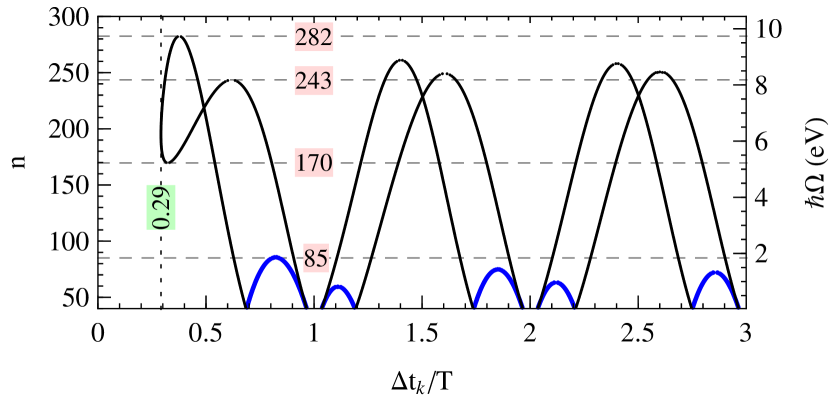
Figure 1: The dependence of $\hbar\Omega$ ($=E_{i}-E_{f}+n\hbar\omega$) on the electron’s travel time $\Delta t_{k}=|t_{k}-t_{k}^{\prime}|$ along various closed trajectories for a laser field with $I=1.06\times 10^{10}$ W/cm², $\hbar\omega=0.04$ eV, $T=2\pi/\omega$ and for initial and final electrons having ${\bf p}_{i}\parallel{\bf p}_{f}\parallel{\bf e}_{z}$, $E_{i}=3.47$ eV, $E_{f}=5.03$ eV. The thick blue lines are for the rescattering scenario I, $\hbar\Omega=\mathcal{E}_{1}(t_{k})$; the thin black lines are for the rescattering scenario II, $\hbar\Omega=\mathcal{E}_{2}(t_{k})$. The vertical line indicates the minimal travel time, corresponding to the shortest closed trajectory; the horizontal lines indicate some local extrema of $\mathcal{E}_{1,2}(t_{k})$ with $\Delta t_{k}<T$.

Figure 1 shows the BrS photon energy $\hbar\Omega=\mathcal{E}_{1,2}(t_{k})$ as a function of the electron’s travel time $\Delta t_{k}=|t_{k}-t_{k}^{\prime}|$ along various closed trajectories in accordance with the previously-described rescattering scenarios. A two-valued dependence of $\mathcal{E}_{2}(t_{k})$ on $\Delta t_{k}$ is due to the character of solutions of the saddle point equation (35), i.e. the numerical analysis of this equation shows that we have two rescattering times $t^{\prime}_{k}(t)$ for a given time $t$ of the first scattering event. As may be seen in figure 1, while $\mathcal{E}_{1}(t_{k})$ is a single-valued function of $\Delta t_{k}$, the dependence of $\mathcal{E}_{2}(t_{k})$ on $\Delta t_{k}$ exhibits the single local minimum ($n=170$) near the shortest closed trajectory with $\Delta t_{k}\approx 0.29T$ ($T=2\pi/\omega$) and a set of local maxima. The first maximum ($n=282$ or $\hbar\Omega_{\max}=9.74$ eV) at $\Delta t_{k}\approx 0.38T$ is a global maximum of $\mathcal{E}_{2}(t_{k})$ and it determines the upper bound of $\Omega$, at which real solutions $\mathcal{P}_{k}$ of the equations (35) and (54) (corresponding to closed classical trajectories) exist. With decreasing $n$, the number of closed classical trajectories increases by the addition of two real solutions each time one crosses a local maximum of $\mathcal{E}_{2}(t)$. We expect that the trajectories related to the first (global) and second (at $\Delta t_{k}\approx 0.61T$) maxima should contribute to the LABrS amplitude significantly, while all other trajectories corresponding to local maxima for $\Delta t_{k}>T$ contribute less. The scenario I (with spontaneous photon emission during the rescattering event) describes the plateau structure for $\hbar\Omega$ smaller than the global maximum of $\mathcal{E}_{1}(t_{k})$ at $\Delta t_{k}=0.84T$, i.e. only for $n\leqslant 85$ or $\hbar\Omega<1.86$ eV.

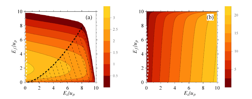
Figure 2: (Color online) Maxima of the emitted energy (in units of $u_{p}$) in accordance with the rescattering scenarios I [$\max\mathcal{E}_{1}$ in panel (a)] and II [$\max\mathcal{E}_{2}$ in panel (b)] as a function of initial, $E_{i}$, and final, $E_{f}$, electron energies for the parallel geometry, ${\bf p}_{i}\|{\bf p}_{f}\|{\bf e}_{z}$. The black dashed line indicates the boundary of the region (indicated by the shaded area below this line) for which the cutoff position of the “direct” LABrS plateau is greater than $\max\mathcal{E}_{1}$. The white dashed lines in (a) and (b) indicate the boundary of the region (left of the line) in which $\max\mathcal{E}_{1}>\max\mathcal{E}_{2}$.

In order to estimate the relative contributions of the rescattering amplitudes ${\bf d}_{n}^{{(\mathrm{rsc}1)}}$ and ${\bf d}_{n}^{{(\mathrm{rsc}2)}}$ for the rescattering scenarios I and II for different initial and final electron energies, in figure 2 we compare the global maxima $\max\mathcal{E}_{1,2}$ of the emitted energies $\mathcal{E}_{1}(t)$ and $\mathcal{E}_{2}(t)$ corresponding to scenarios I and II respectively. As figure 2 shows, the scenario I [panel (a)] considerably contributes over a bounded region of initial ($E_{i}$) and final ($E_{f}$) electron energies limited by the value $10u_{p}$. Moreover, in the region $E_{f}\lesssim E_{i}$ the amplitude ${\bf d}_{n}^{{(\mathrm{dr})}}$ for the direct LABrS exceeds the amplitude ${\bf d}_{n}^{{(\mathrm{rsc}1)}}$ for the rescattering term, i.e., for this region the maximum classically-allowed energy $\hbar\Omega^{{(\mathrm{dr})}}_{\max}$ for the direct process [14] exceeds the value $\max\mathcal{E}_{1}$. The maximal classically-allowed emitted energy $\max\mathcal{E}_{1}\approx 3.16u_{p}$ in accordance with the scenario I appears for low energies $E_{i}\to 0$ and for $E_{f}\approx 1.82u_{p}$. For the scenario II in figure 2(b), the initial energy $E_{i}$ is unlimited, while $E_{f}<10u_{p}$. The maximal emitted energy $\max\mathcal{E}_{2}$ increases with increasing $E_{i}$ and achieves greater values than for the case of scenario I. Only in the tiny region $E_{i}\lesssim 0.2u_{p}$, $E_{f}\lesssim 8u_{p}$ (bounded by the dashed white lines in figure 2) does the amplitude ${\bf d}_{n}^{{(\mathrm{rsc}1)}}$ exceed that of ${\bf d}_{n}^{{(\mathrm{rsc}2)}}$.

3.5 Contributions of coalescing trajectories to the LABrS amplitude

Local extrema of the functions $\mathcal{E}_{1,2}(t)$ [defined in equations (53) and (55)] at $t=\overline{t}_{\nu}$ ($\nu=1,2,\ldots$) correspond to critical values of the emitted photon energy $\hbar\overline{\Omega}_{\nu}$. For example, let $\max[\mathcal{E}_{j}(t)]_{\nu}=\hbar\overline{\Omega}_{\nu}$ ($j=1$ or 2) be the $\nu$th local maximum of the function $\mathcal{E}_{j}(t)$ (similar reasoning may be used for a local minimum), and let $\mathcal{P}_{k_{1}}$ and $\mathcal{P}_{k_{2}}$ be the two nearest real saddle points for $\Omega\lesssim\overline{\Omega}_{\nu}$, cf. figure 1. These saddle points correspond to two closed electron trajectories in the laser field, which coalesce at $\Omega\to\overline{\Omega}_{\nu}$: $\mathcal{P}_{k_{1}}\to\overline{\mathcal{P}}_{\nu}$, $\mathcal{P}_{k_{2}}\to\overline{\mathcal{P}}_{\nu}$ [where $\overline{\mathcal{P}}_{\nu}=(\overline{t}_{\nu},\overline{t^{\prime}}_{\nu})$ is the point of coalescence]. For $\Omega>\overline{\Omega}_{\nu}$, the considered saddle points $\mathcal{P}_{k_{1}}$ and $\mathcal{P}_{k_{2}}$ become complex. The merging of two trajectories $\mathcal{P}_{k_{1}}$ and $\mathcal{P}_{k_{2}}$ at extrema of the emitted energies $\mathcal{E}_{1,2}(t)$ is related to the vanishing of the second derivative (51) of the phase function $\phi(t,t_{k}^{\prime}(t))$:

$$\mathcal{K}_{\mathbf{p}_{i},\mathbf{p}_{f}}(t,t^{\prime}_{k}(t))=0,$$ (57)

$$\mathcal{K}_{-\mathbf{p}_{f},-\mathbf{p}_{i}}(-t,-t^{\prime}_{k}(t))=0.$$ (58)

Equations (57) and (58) correspond to the results (48) for $\mathbf{d}_{n}^{{(\mathrm{rsc}1)}}$ and (49) for $\mathbf{d}_{n}^{{(\mathrm{rsc}2)}}$ respectively. Hence, the merging point $\overline{\mathcal{P}}_{\nu}$ is a solution of the coupled system of equations (34) and (57) [or (35) and (58)].

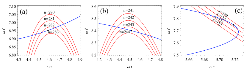
Figure 3: (Color online) The saddle point trajectories in the plane of times ($t,t^{\prime}$) for the rescattering scenario II. The crossings of the blue and red lines give the pairs of saddle points $\mathcal{P}_{k}=(t_{k},t^{\prime}_{k})$. The parameters of the initial and final electrons and of the laser field are the same as in figure 1. Trajectories for $\hbar\Omega$ near two maxima of $\mathcal{E}_{2}(t_{k})$: (a) $n=282$ ($\hbar\Omega=9.74$ eV) and (b) $n=243$ ($\hbar\Omega=8.2$ eV); (c) trajectories near the local minimum of $\mathcal{E}_{2}(t_{k})$ at $n=170$ ($\hbar{\Omega}=5.22$ eV). The blue and red lines indicate solutions of the saddle point equations (35) and (54) respectively. The black points indicate the merging points $\overline{\mathcal{P}}_{\nu}$ [which are solutions of equations (35) and (58)] for two coalescing saddle points.

In figure 3 we illustrate the motion of the saddle points $\mathcal{P}_{k}$ on the plane $(t,t^{\prime})$ with varying $\hbar\Omega$ (or, equivalently, $n$) for the fixed initial $E_{i}$ and final $E_{f}$ electron energies for the case of rescattering scenario II. The blue and red lines in figure 3 indicate solutions of equations (35) and (54) respectively, while their crossing points are the saddle points $\mathcal{P}_{k}$. As shown in figures 3(a) and 3(b), these points move toward each other with increasing $n$, which corresponds to the approach of the function $\mathcal{E}_{2}(t)$ to its local maxima in the vicinity of $n=282$ [figure 3(a)] and $n=243$ [figure 3(b)]. Figure 3(c) illustrates the merging of the pair of saddle points with decreasing $n$ down to $n=170$ and the approach of the local minimum of $\mathcal{E}_{2}(t)$ at $\omega t\approx 5.72$. In the vicinity of this time, the solution $t^{\prime}_{k}(t)$ of (35) (the blue line) exhibits a branch point (at $t=\tilde{t}$ ), which means that the second partial derivative of the phase function $\varphi_{\bf p}(t,t^{\prime})$ [given by expression (20)] over $t^{\prime}$ vanishes at this point, i.e., $\mathcal{D}_{\mathbf{p}}(\tilde{t},t^{\prime}_{k}(\tilde{t}\,))=0$ [$\mathcal{D}_{\bf p}(t,t^{\prime}_{k}(t))\sim(dt^{\prime}_{k}/dt)^{-1}$]. For coalescing saddle points, the saddle point analysis used to obtain the rescattering expansion for the function $f_{\bf p}(t)$ [cf. equation (14)] is not applicable and leads to incorrect results.

To take into account the coalescence of the $k_{1}$th and $k_{2}$th saddle points (and hence to apply our results for the vicinity of the critical value $\overline{\Omega}_{\nu}$ of the BrS photon frequency $\Omega$), we modify the regular saddle point method for analysis of the integral in (43) by making use of the general idea of the uniform approximation [24, 25]. We need only evaluate the integral of the first term ($\bm{\mathcal{D}}$) in (43), since the result for the integral of the second term ($\bm{\mathcal{D}}|_{\mathcal{G}}$) can be found by replacing the parameters (33) in the result obtained for $\bm{\mathcal{D}}$. We approximate the phase function $\phi(t,t^{\prime}_{k}(t))$ in (45) in the vicinity of $t=\overline{t}_{\nu}$ by the following cubic polynomial:

$$\phi(t,t^{\prime}_{k}(t))=\overline{\phi}+\phi_{1}\omega(t-\overline{t}_{\nu})+(\phi_{2}/3)[\omega(t-\overline{t}_{\nu})]^{3},$$ (59)

where $\overline{\phi}\equiv\phi(\overline{t}_{\nu},\overline{t^{\prime}}_{\nu})$ and the coefficients $\phi_{1}$ and $\phi_{2}$ are expressed in terms of the first and third derivatives of the function $\phi(t,t^{\prime}_{k}(t))$ over $t$ evaluated at the point $t=\overline{t}_{\nu}$ [where we denote $\overline{t^{\prime}}_{\nu}\equiv t_{k}^{\prime}(\overline{t}_{\nu})$]: $\phi_{1}=d\phi/(\omega dt)|_{t=\overline{t}_{\nu}}$, $\phi_{2}=d^{3}\phi/(2\omega^{3}dt^{3})|_{t=\overline{t}_{\nu}}$. The explicit expressions for $\phi_{1}$ and $\phi_{2}$ are:

$$\phi_{1}=\frac{\Omega-\overline{\Omega}_{\nu}}{\omega},\quad\overline{\Omega}_{\nu}=\frac{\mathbf{Q}^{2}(\overline{t}_{\nu},\overline{t^{\prime}}_{\nu})-\mathbf{P}_{f}^{2}(\overline{t}_{\nu})}{2m\hbar},$$ (60)

$$\phi_{2}=\frac{2u_{p}}{\hbar eF}\mathbf{e}_{z}\cdot[\mathbf{p}_{f}-\mathbf{q}(\overline{t}_{\nu},\overline{t^{\prime}}_{\nu})]\left(\mathcal{B}-\sin\omega\overline{t}_{\nu}\right),$$ (61)

$$\mathcal{B}=\frac{\left[(\mathbf{e}_{z}\cdot\mathbf{Q}(\overline{t^{\prime}}_{\nu},\overline{t}_{\nu}))^{3}\sin\omega\overline{t^{\prime}}_{\nu}+\mathcal{C}\right]\cos^{2}\omega\overline{t}_{\nu}}{\beta(\mathbf{e}_{z}\cdot\mathbf{Q}(\overline{t}_{\nu},\overline{t^{\prime}}_{\nu}))^{3}\cos^{2}\omega\overline{t^{\prime}}_{\nu}},$$

$$\mathcal{C}=\frac{3eF}{\omega}\big{[}\mathbf{Q}(\overline{t^{\prime}}_{\nu},\overline{t}_{\nu})\cdot\mathbf{P}_{i}(\overline{t^{\prime}}_{\nu})$$

$$\phantom{C}-\beta\mathbf{Q}(\overline{t}_{\nu},\overline{t^{\prime}}_{\nu})\cdot\mathbf{P}_{f}(\overline{t}_{\nu})\big{]}\cos^{2}\omega\overline{t^{\prime}}_{\nu},$$

$$\beta=\left(\frac{\mathbf{e}_{z}\cdot[\mathbf{p}_{i}-\mathbf{q}(\overline{t}_{\nu},\overline{t^{\prime}}_{\nu})]}{\mathbf{e}_{z}\cdot[\mathbf{p}_{f}-\mathbf{q}(\overline{t}_{\nu},\overline{t^{\prime}}_{\nu})]}\right)^{2}\frac{\cos\omega\overline{t^{\prime}}_{\nu}}{\cos\omega\overline{t}_{\nu}}.$$

In the vicinity of the point $\overline{t}_{\nu}$, we approximate the pre-exponential factor $\bm{\mathcal{F}}$ in (44) by the linear polynomial:

$$\bm{\mathcal{F}}(t,t^{\prime}_{k}(t))=\bm{c}_{0}+\bm{c}_{1}\omega(t-\overline{t}_{\nu}).$$ (62)

The coefficients $\bm{c}_{0}$ and $\bm{c}_{1}$ are expressed in terms of the values of the function $\bm{\mathcal{F}}(t,t^{\prime})$ taken at two close saddle points $t_{k_{1}}$, $t_{k_{2}}$ [$\bm{\mathcal{F}}_{k}\equiv\bm{\mathcal{F}}(t_{k},t^{\prime}_{k})$, $k=k_{1},k_{2}$]:

$$\bm{c}_{0}=\frac{(t_{k_{2}}-\overline{t}_{\nu})\bm{\mathcal{F}}_{k_{1}}-(t_{k_{1}}-\overline{t}_{\nu})\bm{\mathcal{F}}_{k_{2}}}{t_{k_{2}}-t_{k_{1}}},$$

$$\bm{c}_{1}=\frac{\bm{\mathcal{F}}_{k_{2}}-\bm{\mathcal{F}}_{k_{1}}}{\omega(t_{k_{2}}-t_{k_{1}})}.$$

Substituting the expressions (59) and (62) into (44) and extending the range of integration over $t$ to $(-\infty,\infty)$, the integral in (43) can be evaluated analytically in terms of the Airy function $\mathrm{Ai}(x)$ and its derivative $\mathrm{Ai}^{\prime}(x)$:

$$\frac{1}{2\pi}\int_{-\infty}^{\infty}dx(\bm{c}_{0}+\bm{c}_{1}x)e^{i(\overline{\phi}+\phi_{1}x+\phi_{2}x^{3}/3)}$$

$$=e^{i\overline{\phi}}\eta\Big{[}\bm{c}_{0}\mathrm{Ai}\left(\hat{s}\eta\phi_{1}\right)-i\bm{c}_{1}\hat{s}\eta\mathrm{Ai}^{\prime}\left(\hat{s}\eta\phi_{1}\right)\Big{]},$$ (63)

where $\eta=|\phi_{2}|^{-1/3}$, $\hat{s}=\mathrm{sgn}(\phi_{2})$, $\mathrm{sgn}(x)=\pm 1$ for $x\gtrless 0$. Finally, the corrected result for the contribution $\mathbf{d}^{{(\mathrm{rsc}1)}}_{n,\nu}$ of two real coalescing saddle points with $k=k_{1}$ and $k_{2}$ [which are involved in the rescattering LABrS dipole moment $\mathbf{d}^{{(\mathrm{rsc}1)}}_{n}$ in (48)] can be presented in the form:

$$\mathbf{d}^{{(\mathrm{rsc}1)}}_{n,\nu} = \frac{\eta e^{i\overline{\phi}}}{\omega(t_{k_{2}}-t_{k_{1}})}\sum_{j=0,1}(-1)^{j}\bm{\mathcal{F}}_{k_{j+1}}$$ (64)

$$\times \left[\omega(t_{k_{2-j}}-\overline{t}_{\nu})\mathrm{Ai}(\xi_{\nu})+i\hat{s}\eta\mathrm{Ai}^{\prime}(\xi_{\nu})\right],$$

where

$$\xi_{\nu}=\hat{s}\eta(\Omega-\overline{\Omega}_{\nu})/\omega.$$ (65)

Approximating the merging point $\overline{t}_{\nu}$ in (64) by the center of the interval $(t_{k_{1}},t_{k_{2}})$, $\overline{t}_{\nu}\approx(t_{k_{1}}+t_{k_{2}})/2$ (which is a reasonable approximation in the vicinity of local maxima of the functions $\mathcal{E}_{1,2}(t)$, cf. figures 1 and 3), for $\mathbf{d}^{{(\mathrm{rsc}1)}}_{n,\nu}$ we obtain

$$\mathbf{d}^{{(\mathrm{rsc}1)}}_{n,\nu} = \sum_{j=1}^{2}\mathbf{d}^{(0)}\big{[}\mathbf{Q}(t_{k_{j}},t_{k_{j}}^{\prime}),\mathbf{P}_{f}(t_{k_{j}})\big{]}$$ (66)

$$\times \mathcal{A}\big{[}P_{i}(t^{\prime}_{k_{j}})\big{]}\mathcal{W}_{k_{j}}^{(\nu)},$$

where the propagation factors $\mathcal{W}_{k_{j}}^{(\nu)}$ have the following form:

$$\mathcal{W}_{k}^{(\nu)} = \frac{\eta e^{i\overline{\phi}}}{2\sqrt{(\hbar/m)({t}_{k}-{t^{\prime}}_{k})^{3}\mathcal{D}_{\mathbf{p}_{i}}({t}_{k},{t^{\prime}}_{k})}}$$ (67)

$$\times \left[\mathrm{Ai}(\xi_{\nu})-\frac{i\hat{s}\eta}{\omega(t_{k}-\overline{t}_{\nu})}\mathrm{Ai}^{\prime}(\xi_{\nu})\right].$$

The result for $\mathbf{d}^{{(\mathrm{rsc}2)}}_{n,\nu}$ follows from the results (66) and (67) by the following set of substitutions: $\mathcal{G}=\{{\bf p}_{i}\leftrightarrow-{\bf p}_{f},\mathcal{P}_{k}\to-\mathcal{P}_{k},\overline{\mathcal{P}}_{\nu}\to-\overline{\mathcal{P}}_{\nu}\}$ [cf. (33)], where the saddle points $\mathcal{P}_{k}=(t_{k},t_{k}^{\prime})$ satisfy the system of equations (35) and (54) and the merging point $\overline{\mathcal{P}}_{\nu}=(\overline{t}_{\nu},\overline{t^{\prime}}_{\nu})$ is a solution of the system of equations (35) and (58):

$$\mathbf{d}^{{(\mathrm{rsc}2)}}_{n,\nu} = \sum_{j=1}^{2}\mathbf{d}^{(0)}\big{[}\mathbf{P}_{i}(t_{k_{j}}),\mathbf{Q}(t_{k_{j}},t_{k_{j}}^{\prime})\big{]},$$ (68)

$$\times \mathcal{A}[P_{f}(t^{\prime}_{k_{j}})]\mathcal{W\,^{\prime}}_{k_{j}}^{(\nu)},$$

where $\mathcal{W\,^{\prime}}_{k}^{(\nu)}=\mathcal{W}_{k}^{(\nu)}\big{|}_{\mathcal{G}}$.

The result (66) [or (68)] describes the contributions of two real coalescing saddle points $\mathcal{P}_{k_{1}}$ and $\mathcal{P}_{k_{2}}$, corresponding to two terms in (48) [or (49)] with $k=k_{1},k_{2}$. As discussed above, these two solutions become complex for $\hbar\Omega$ greater than the local maximum of the function $\mathcal{E}_{1}(t)$ [or $\mathcal{E}_{2}(t)$] or for $\hbar\Omega$ smaller than the local minimum of $\mathcal{E}_{1}(t)$ [or $\mathcal{E}_{2}(t)$], while in (48) [or (49)] we take into account only one of them, which describes the decrease of the partial LABrS amplitude as $\Omega$ varies. In order to obtain the result for this term in the vicinity of the critical value $\overline{\Omega}_{\nu}$, we first simplify the results (66) and (68). We first approximate the pre-exponential factor $\bm{\mathcal{F}}(t,t^{\prime})$ by its value at $t=\overline{t}_{\nu}$ , i.e. we use equation (62) with $\bm{c}_{0}=\bm{\mathcal{F}}(\overline{t}_{\nu},\overline{t^{\prime}}_{\nu})$ and $\bm{c}_{1}=0$. Using then (63), we obtain that the two terms in the sum for $\mathbf{d}_{n,\nu}^{{(\mathrm{rsc}1)}}$ in (66) [and similarly for $\mathbf{d}_{n,\nu}^{{(\mathrm{rsc}2)}}$ in (68)] can be replaced by only one term with $\mathcal{P}_{k_{1}}=\mathcal{P}_{k_{2}}=\overline{\mathcal{P}}_{\nu}$:

$$\mathbf{d}^{{(\mathrm{rsc}1)}}_{n,\nu}=\mathbf{d}^{(0)}\big{[}\mathbf{Q}^{(\nu)},\mathbf{P}_{f}^{(\nu)}\big{]}\mathcal{A}\big{[}P_{i}^{\prime(\nu)}\big{]}\mathcal{W}^{(\nu)},$$ (69)

$$\mathbf{d}^{{(\mathrm{rsc}2)}}_{n,\nu}=\mathbf{d}^{(0)}\big{[}\mathbf{P}_{i}^{(\nu)},\mathbf{Q}^{(\nu)}\big{]}\mathcal{A}\big{[}P_{f}^{\prime(\nu)}\big{]}\mathcal{W\,^{\prime}}^{(\nu)},$$ (70)

where $\mathbf{Q}^{(\nu)}=\mathbf{Q}(\overline{t}_{\nu},\overline{t^{\prime}}_{\nu})$, $\mathbf{P}_{i,f}^{(\nu)}=\mathbf{P}_{i,f}(\overline{t}_{\nu})$, $P_{i,f}^{\prime(\nu)}=P_{i,f}(\overline{t^{\prime}}_{\nu})$ and the propagation factors are

$$\mathcal{W}^{(\nu)}=\frac{\overline{\Omega}_{\nu}^{2}\eta e^{i\overline{\phi}}\mathrm{Ai}(\xi_{\nu})}{\Omega^{2}\sqrt{(\hbar/m)(\overline{t}_{\nu}-\overline{t^{\prime}}_{\nu})^{3}\mathcal{D}_{\mathbf{p}_{i}}(\overline{t}_{\nu},\overline{t^{\prime}}_{\nu})}},$$ (71)

$$\mathcal{W\,^{\prime}}^{(\nu)}=\mathcal{W}^{(\nu)}|_{\mathcal{G}}.$$ (72)

The simplified results (69) and (70) depend only on the real merging point $\overline{\mathcal{P}}_{\nu}$, and thus they can be used in the classically-forbidden region of $\Omega$ (i.e., where the saddle points $\mathcal{P}_{k}$ become complex). We emphasize that the atomic factors $\mathcal{A}$ and $\mathbf{d}^{(0)}$ in (69) and (70) depend on the real kinetic momenta taken at the real times $\overline{t}_{\nu}$ and $\overline{t^{\prime}}_{\nu}$.

For an accurate description of the high-energy (or rescattering) part of the LABrS spectrum in the low-frequency approximation, we use the following rules: (i) For the interval $x_{0}<\eta(\Omega-\overline{\Omega}_{\nu})/\omega<0$, where $x_{0}\approx-2.34$ is the first zero of the Airy function for negative arguments ($\mathrm{Ai}(x_{0})=0$), we replace two terms in the expression (48) [(49)] with coalescing saddle points at local maxima $\hbar\overline{\Omega}_{\nu}$ of the function $\mathcal{E}_{1}(t)$ [$\mathcal{E}_{2}(t)$] by the result (66) [(68)]; (ii) For $\Omega>\overline{\Omega}_{\nu}$ (i.e. for energies $\hbar\Omega$ exceeding a local maximum of $\mathcal{E}_{1,2}$), we replace a term in (48) [(49)], originating from the coalescence of two real trajectories, by the result (69) [(70)]; (iii) In the vicinity of the local minimum of the function $\mathcal{E}_{2}(t)$ (cf. discussions of figures 1 and 3) we extend the use of the simplified result (70) into the region of the singularity of the function $f_{-{\bf p}_{f}}(t)$ ($\mathcal{D}_{-{\bf p}_{f}}\approx 0$); (iv) Except for these special cases (i-iii), the rescattering results (48) and (49) (obtained in the nonresonant low-frequency approximation) are used. Note that the partial LABrS amplitudes in expressions (48) and (49) corresponding to complex saddle points $\mathcal{P}_{k}$ (far away from a coalescence point) can be evaluated directly [without simplification to the forms (69) and (70)] using the analytic functions $\mathcal{A}$ and ${\bf d}^{(0)}$ obtained within the effective range approximation.

4 Numerical results and discussion

4.1 Comparisons with exact TDER results and discussions of interference phenomena

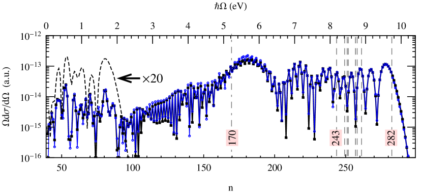
Figure 4: (Color online) Spectral density of laser-assisted $e$-H BrS as a function of the number $n$ of laser photons absorbed for the same parameters of the initial and final electrons and the laser field as in figure 1. Thick (black) line with squares – exact TDER results; thin (blue) line with circles – results for nonresonant rescattering in the low-frequency approximation; thin dashed (black) line – results obtained using (48), (68) and (70); the vertical gray lines indicate extremal values of $\overline{\Omega}_{\nu}$: dashed lines – local maxima of $\mathcal{E}_{2}(t)$, dot-dashed line – a local minimum of $\mathcal{E}_{2}(t)$.

The LABrS spectral density $\Omega d\sigma/d\Omega$ [cf. (4)] as a function of the emitted photon energy $\hbar\Omega$ (or the number $n$ of laser photons exchanged) is presented in figure 4. One sees that the LABrS spectrum clearly exhibits a plateau structure: $\Omega d\sigma/d\Omega$ is an oscillating function for a broad interval of frequencies $\Omega<\Omega_{\max}$ (where $\Omega_{\max}\approx 9.6$ eV defines the plateau cutoff), while beyond the cutoff (for $\Omega>\Omega_{\max}$) the spectral density decays rapidly. Figure 4 shows the good agreement of our analytic low-frequency results [i.e., the results (48) and (49) and their further modifications in section 3.5] with the exact numerical TDER results (cf. the discussion of equations (12) and (13) in section 2).

The oscillation patterns of the LABrS cross section originate from interference of partial amplitudes given by different summands in (48) and (49). The contributions of the “direct” term $\mathbf{d}_{n}^{{(\mathrm{dr})}}$ in figure 4 are negligible. The rescattering term $\mathbf{d}_{n}^{{(\mathrm{rsc}1)}}$ (which corresponds to spontaneous emission upon electron-atom rescattering) plays a role in the low-energy part of the spectrum, where this term interferes with $\mathbf{d}_{n}^{{(\mathrm{rsc}2)}}$ (cf. the dashed line in figure 4, which for visibility gives the contribution of the amplitude $\mathbf{d}_{n}^{{(\mathrm{rsc}1)}}$ multiplied by a factor of 20). Therefore, the plateau-like behavior of the LABrS spectrum is mainly described by the amplitude $\mathbf{d}_{n}^{{(\mathrm{rsc}2)}}$, which corresponds to the rescattering scenario II, with spontaneous photon emission at the first electron-atom collision. There are only two real saddle points $\mathcal{P}_{1}$ and $\mathcal{P}_{2}$ (i.e., only two terms in the sum for $\mathbf{d}_{n}^{{(\mathrm{rsc}2)}}$) in the plateau cutoff region. These two saddle points coalesce [$\mathcal{P}_{1}\to\overline{\mathcal{P}}_{1}$, $\mathcal{P}_{2}\to\overline{\mathcal{P}}_{1}$] for $\Omega=\overline{\Omega}_{1}\equiv\Omega_{\max}=9.74$ eV or $n_{\max}=282$ [cf. figures 3(a) and 1]. Therefore, the LABrS amplitude near the rescattering plateau cutoff is well approximated by the result (68), $\mathbf{d}_{n}^{{(\mathrm{rsc}2)}}\approx\overline{\mathbf{d}}_{n,1}^{{(\mathrm{rsc}2)}}$. The few oscillation maxima of the spectral density closest to the cutoff are described by the Airy function and its derivative [involved in the propagation factors $\mathcal{W^{\prime}}_{k_{1,2}}^{(\nu)}$ in (68)], which oscillate for negative arguments, $\Omega<\overline{\Omega}_{1}$ [cf. (65)]. For smaller energies $\hbar\Omega$, the number of saddle points one must take into account increases (cf. the LABrS spectrum region $\hbar\Omega\lesssim 9$ eV in figure 4, in which the vertical dashed lines indicate the appearance of pairs of real saddle points), while the accuracy of the result (68) worsens. As mentioned above, the contributions of partial amplitudes with different travel times $\Delta t_{k}=|t_{k}^{\prime}-t_{k}|$ decreases with increasing $\Delta t_{k}$. We do not take into account saddle points ($t_{k},t^{\prime}_{k}$) that describe long closed trajectories having traveling times $\Delta t_{k}>4T$ since the main contributions are given by the relatively few trajectories with $\Delta t_{k}<T$. In figure 4, the appearance of two real saddle points for $n<243$ (these solutions correspond to closed trajectories with short travel times $\sim 0.6T$, cf. figure 1) leads to strong interference of the corresponding partial amplitudes with other terms in (49) and, hence, to the appearance of high-frequency oscillations in LABrS spectra.

For 5.2 eV $\lesssim\hbar\Omega\lesssim 6$ eV, the LABrS spectral density in figure 4 exhibits a pronounced enhancement (similar to an interference maximum in the cutoff region). This enhancement is due to the interference of two coalescing trajectories in the vicinity of the local minimum of the function $\mathcal{E}_{2}(t)$, $\hbar\overline{\Omega}_{\nu}=5.2$ eV (cf. figure 1). The relative suppression of the LABrS cross section occurs for $\hbar\Omega\lesssim 5$ eV, because the shortest real trajectories disappear in this region (cf. the black curves in figure 1).

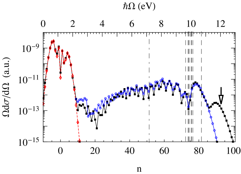
Figure 5: (Color online) The same as in figure 4 but for LABrS in a CO₂ laser field with $\hbar\omega=0.117$ eV, $I=6.4\times 10^{10}$ W/cm², $E_{i}=4.84$ eV and $E_{f}=3.67$ eV. Dashed (red) line with diamonds is the ‘direct’ LABrS result (29). The arrow indicates the cutoff of the resonant rescattering plateau in accordance with (73).

In figure 5 we present the $e$-H LABrS spectrum for the case of a CO₂ laser field with $\hbar\omega=0.117$ eV and intensity $I=6.4\times 10^{10}$ W/cm². The low-energy part of the spectrum (for $\hbar\Omega<2$ eV) represents a plateau-like structure and is well described by the “direct” part $\mathbf{d}_{n}^{{(\mathrm{dr})}}$ of the LABrS amplitude. The second (high-energy) plateau for 2.5 eV$<\hbar\Omega<11$ eV is described by the rescattering amplitude $\mathbf{d}_{n}^{{(\mathrm{rsc}2)}}$, while the contribution of the amplitude $\mathbf{d}_{n}^{{(\mathrm{rsc}1)}}$ is negligible and is masked by the “direct” LABrS plateau. The averaged value of the spectral density along the rescattering plateau is about 2 – 3 orders of magnitude smaller than for the “direct” plateau, in agreement with the fact that the relative magnitude of the amplitudes $\mathbf{d}_{n}^{{(\mathrm{rsc})}}$ and $\mathbf{d}_{n}^{{(\mathrm{dr})}}$ is governed by the parameter $\mathcal{A}/\alpha_{0}$, which is the ratio of the characteristic field-free scattering amplitude $\mathcal{A}$ to the quiver radius, $\alpha_{0}=|e|F/(m\omega^{2})$, of a free electron in the laser field. Indeed, it follows from (48) and (49) that the rescattering amplitude $\mathbf{d}_{n}^{{(\mathrm{rsc})}}$ contains an additional factor $\sim\mathcal{A}/\alpha_{0}$ [the propagation factors $\mathcal{W}_{k}$ and $\mathcal{W}_{k}^{\prime}$ are proportional to $\alpha_{0}^{-1}$, cf. (50)] in comparison with $\mathbf{d}_{n}^{{(\mathrm{dr})}}$ (cf. also the low-frequency analysis of the LAES process in [18]). For low-energy $e$-H scattering within the effective range theory, $\mathcal{A}\approx a_{0}=6.2$ a.u., while $\alpha_{0}=73$ a.u. for the parameters of the spectrum in figure 5. The strong enhancement of the spectral density beyond the rescattering plateau cutoff (for $\hbar\Omega>11$ eV) is related to resonant LABrS due to radiative recombination into an intermediate quasibound state of the H^- ion [14]. As shown in [14] (cf. also [28, 29]), the cutoff of the LARA/LARR process is determined by the relation:

$$\hbar\Omega^{(r)}=\frac{1}{2m}\left(\mathbf{p}_{i}+\mathrm{sgn}(\mathbf{p}_{i}\cdot\mathbf{e}_{z})\mathbf{e}_{z}\frac{|e|F}{\omega}\right)^{2}+|E_{0}|,$$ (73)

where $E_{0}$ is the energy of the bound state. For the parameters applicable to figure 5 and $E_{0}=-0.755$ eV (the ground state energy of H^-), equation (73) gives $\hbar\Omega^{(r)}=12.04$ eV, which coincides with the cutoff of the “extended” plateau in figure 5. The disagreement of the nonresonant low-frequency results with the exact TDER theory results for energies 2.5 eV$<\hbar\Omega<4$ eV (where the LABrS spectrum exhibits a suppression similar to the suppression in figure 4 for 2 eV$<\hbar\Omega<4$ eV) is also caused by the previously discussed resonant channel.

4.2 Estimate of the LABrS cross section for electron scattering from a Coulomb potential

Since the analytic results (29), (48) and (49) contain field-free atomic factors evaluated at laser-modified instantaneous momenta, they allow one to extend their applicability beyond the assumptions of the TDER theory. This extension is very straightforward and consists in the replacement of the atomic factors $\mathcal{A}$ and $\mathbf{d}_{0}$ obtained within the TDER approach by their counterparts for a real atomic potential. We emphasize that the propagation factors $\mathcal{W}_{k}$ and $\mathcal{W}_{k}^{\prime}$ (that describe key aspects of rescattering in the LABrS process) do not involve any information about electron-atom interactions and are general for any atomic target. In figure 6 we present LABrS spectra for the case of the electron-Coulomb interaction, i.e. for electron-proton BrS. The field-free quantities for this case are the electron-Coulomb scattering amplitude $\mathcal{A}$, obtained from [26], and the BrS dipole moment $\mathbf{d}_{0}$, obtained from [27]. In figure 6 we present results for two different sets of laser field parameters: (1) $\lambda=1064$ nm, $I=8\times 10^{13}$ W/cm² and (2) $\lambda=532$ nm, $I=3.2\times 10^{14}$ W/cm², such that the ratio $F/\omega$ is the same, while the quiver radius $\alpha_{0}$ changes by a factor of 2. We note that both parameters $\omega p_{i}/(|e|F)=2.2$ and $\omega p_{f}/(|e|F)=1.6$ are greater than one; if they were less than one the electron momenta $P_{i,f}(t^{\prime}_{k})$ in the Coulomb scattering amplitude might vanish, so that the results (48) and (49) would become inapplicable. For the chosen parameters, the saddle points $\mathcal{P}_{k}$ (and field-free amplitudes) are the same in both cases, while the propagation factors differ and cause different oscillation patterns in the LABrS spectra. As is seen in figure 6, for the shorter wavelength (and thus for the smaller quiver radius, $\alpha_{0}\propto\lambda^{2}\sqrt{I}$) the spectral density is approximately 4 times higher.

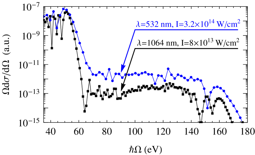
Figure 6: (Color online) Spectral density of electron-proton BrS in laser fields with two different wave lengths $\lambda$ and intensities $I$, as shown in the figure. Incident and final electron parameters: $\mathbf{p}_{i}\|\mathbf{p}_{f}\|\mathbf{e}_{z}$, $E_{i}=80$ eV and $E_{f}=45$ eV.

5 Concluding Summary

In this paper, we have developed an analytic description of the LABrS process taking into account the rescattering effects of the active electron on the atomic target. These effects are responsible for the occurrence of the high-energy plateau in the dependence of the LABrS spectral density on the emitted photon energy (or on the number of laser photons exchanged). The key results of our analytic approach are the expressions (48) and (49), which present the LABrS dipole moment (the LABrS amplitude) in the nonresonant low-frequency approximation. These results have a transparent interpretation in terms of the rescattering scenario. Moreover, these results describe two possible realizations of this scenario, scenario I and scenario II. The result (48) for $\mathbf{d}_{n}^{{(\mathrm{rsc}1)}}$ represents an interference of partial amplitudes, each related to the pair of times $t_{k}$ and $t_{k}^{\prime}$. It describes the following three-step picture (scenario I): (i) the electron elastically scatters from the atom at the moment $t_{k}^{\prime}$, (ii) the laser field returns the electron back to the atom at the moment $t_{k}$ ($t_{k}>t_{k}^{\prime}$), where (iii) the electron rescatters with sponataneous photon emission. Similarly, the result (49) for $\mathbf{d}_{n}^{{(\mathrm{rsc}2)}}$ describes the scenario II: (i) the BrS process happens at the first electron-atom collision at the time $t_{k}$, (ii) the laser field returns the electron back to the atom at the moment $t_{k}^{\prime}$ ($t_{k}^{\prime}>t_{k}$), followed by (iii) the elastic electron scattering (the rescattering event). The pair of times $(t_{k},t_{k}^{\prime})$ corresponds to some closed trajectory of the electron’s motion in the laser field between the events of the first and second electron-atom collisions. We have found that the scenario II with spontaneous photon emission during the first collision is allowed for an arbitrary incident electron energy $E_{i}$. Numerical analysis shows that this scenario is significant for such values of the final electron energy $E_{f}$ that $E_{f}<10u_{p}$. Another situation is realized for the scenario I, with photon emission during the second collision (rescattering). For this case, the dipole moment $\mathbf{d}_{n}^{{(\mathrm{rsc}1)}}$ can contribute to the LABrS amplitude for $E_{i}<10u_{p}$, and exceeds the term $\mathbf{d}_{n}^{{(\mathrm{rsc}2)}}$ only for $E_{i}\lesssim 0.2u_{p}$ (for the case of the parallel geometry ${\bf p}_{i}\|{\bf p}_{f}\|{\bf e}_{z}$). In comparison with the direct LABrS process, the rescattering effects significantly extend the maximum energy of the emitted photon (up to the rescattering plateau cutoff), while the averaged value of the spectral density is about 2 – 3 orders of magnitude smaller than for the direct process. Finally, the clear physical meaning of the key factors involved in the TDER results (48) and (49) allow us to generalize those factors to the case of real atoms or ions. Such generalization has been made for electron-proton LABrS, followed by the numerical evaluation of the LABrS spectral density for this case.

Appendix. Derivation of results (37) and (38) for ${\tilde{\mathbf{d}}_{n}}$

Taking into account (7) and (8), we rewrite the definition (13) for ${\tilde{\mathbf{d}}_{n}}$ in explicit form:

$${{\tilde{\mathbf{d}}_{n}}}=e\left(\frac{2\pi\hbar^{2}}{m\kappa}\right)^{2}\frac{1}{T}\int\limits_{0}^{T}dt\int\limits_{-\infty}^{t}dt^{\prime}\int\limits_{t}^{\infty}dt^{\prime\prime}$$ (74)

$$\times e^{in\omega t+i[\epsilon_{i}(t-t^{\prime})+\epsilon_{f}(t^{\prime\prime}-t)]/\hbar}f_{\mathbf{p}_{i}}(t^{\prime})f_{-\mathbf{p}_{f}}(-t^{\prime\prime})$$

$$\times \int d\mathbf{r}\,G^{(-)*}({\bf r},t;0,t^{\prime\prime})\,\mathbf{r}\,G^{(+)}({\bf r},t;0,t^{\prime}).\hskip 14.22636pt$$

For the spatial integral in (74), we use the following relation (cf. the Appendix in [23]):

$$\int d\mathbf{r}\,G^{(+)}({\bf r},t;0,t^{\prime})\,\mathbf{r}\,G^{(-)*}({\bf r},t;0,t^{\prime\prime})$$

$$=\frac{i}{\hbar}G^{(+)}(0,t^{\prime\prime};0,t^{\prime})\bm{\mathcal{R}}(t;t^{\prime},t^{\prime\prime}),$$

where

$$\bm{\mathcal{R}}(t;t^{\prime},t^{\prime\prime}) = \frac{e}{m\omega^{2}(t^{\prime}-t^{\prime\prime})}\Big{\{}(t-t^{\prime\prime})\big{[}\mathbf{F}(t)-\mathbf{F}(t^{\prime})\big{]}$$

$$- (t-t^{\prime})\big{[}\mathbf{F}(t)-\mathbf{F}(t^{\prime\prime})\big{]}\Big{\}}.$$

In order to treat the three-dimensional integral over $t^{\prime\prime}$, $t^{\prime}$, $t$ in (74), we introduce new variables: $\xi=(t^{\prime\prime}-t^{\prime})/2$, $\zeta=t-(t^{\prime}+t^{\prime\prime})/2$, $\tilde{t}=t-\zeta$ ($0\leqslant\xi<\infty$, $-\xi\leqslant\zeta\leqslant\xi$). Integration over $\zeta$ leads to the result:

$${{\tilde{\mathbf{d}}_{n}}}={{\tilde{\mathbf{d}}_{n}}}^{(+)}+{{\tilde{\mathbf{d}}_{n}}}^{(-)},$$

$${{\tilde{\mathbf{d}}_{n}}}^{(\pm)}=\mp\frac{e^{2}}{2\omega^{2}\Omega}\sqrt{\frac{\pi i\hbar}{m^{3}}}\frac{1}{T}\int_{0}^{T}d\tilde{t}\int\limits_{0}^{\infty}\frac{d\xi}{\xi^{3/2}}e^{\pm i\xi\Omega}$$

$$\times e^{in\omega\tilde{t}+(i/\hbar)\left[(\epsilon_{i}+\epsilon_{f})\xi+S\left(\tilde{t}+\xi,\tilde{t}-\xi\right)\right]}$$

$$\times f_{\mathbf{p}_{i}}\left(\tilde{t}-\xi\right)f_{-\mathbf{p}_{f}}\left(-\tilde{t}-\xi\right)\Bigg{\{}\frac{\mathbf{F}\left(\tilde{t}-\xi\right)-\mathbf{F}\left(\tilde{t}+\xi\right)}{\Omega\xi}$$

$$+2i\mathbf{F}\left(\tilde{t}\pm\xi\right)-i\mathbf{e}_{z}F\sum_{s=\pm 1}\frac{\Omega e^{is\omega(\tilde{t}\pm\xi)}}{\Omega+s\omega}\Bigg{\}}.$$ (75)

Applying the variable replacement $\tilde{t}=t-\xi$ to ${\tilde{\mathbf{d}}_{n}}^{(+)}$ in (75) followed by the replacement $t^{\prime}=t-2\xi$, we obtain for ${{\tilde{\mathbf{d}}_{n}}}^{(+)}$ the expression (37). Similarly, applying the variable replacement $\tilde{t}=t+\xi$ to ${\tilde{\mathbf{d}}_{n}}^{(-)}$ in (75) followed by the replacement $t^{\prime}=t+2\xi$, we obtain the result (38) for ${{\tilde{\mathbf{d}}_{n}}}^{(-)}$.

References

References

• [1] Karapetyan R V and Fedorov M V 1978 Zh. Eksp. Teor. Fiz. 75 816
Karapetyan R V and Fedorov M V 1978 Sov. Phys.–JETP 48 412 (Engl. Transl.)
• [2] Zhou F and Rosenberg L 1993 Phys. Rev. A 48 505
• [3] Kroll N M and Watson K M 1973 Phys. Rev. A 8 804
• [4] Ehlotzky F, Jaroń A and Kamiński J Z 1998 Phys. Rep. 297 63
• [5] Dondera M and Florescu V 2006 Rad. Phys. Chem. 75 1380
• [6] Salières P, Carré B, Le Déroff L, Grasbon F, Paulus G G, Walther H, Kopold R, Becker W, Milošević D B, Sanpera A and Lewenstein M 2001 Science 292 902
• [7] Becker W, Grasbon F, Kopold R, Milošević D B, Paulus G G, and Walther H 2002 Adv. At. Mol. Opt. Phys. 48 35
• [8] Milošević D B and Ehlotzky F 2003 Adv. At. Mol. Opt. Phys. 49 373
• [9] Manakov N L, Starace A F, Flegel A V and Frolov M V 2002 Zh. Eksp. Teor. Fiz. Pis ma Red. 76 316
Manakov N L, Starace A F, Flegel A V and Frolov M V 2002 JETP Lett. 76 258 (Engl. Transl.)
• [10] Čerkić A and Milošević D B 2004 Phys. Rev. A 70 053402
• [11] Milošević D B and Ehlotzky F 2002 Phys. Rev. A 65 042504
• [12] Zheltukhin A N, Manakov N L, Flegel A V and Frolov M V 2011 Zh. Eksp. Teor. Fiz. Pis ma Red. 94 641
Zheltukhin A N, Manakov N L, Flegel A V and Frolov M V 2011 JETP Lett. 94 599 (Engl. Transl.)
• [13] Frolov M V, Manakov N L, Pronin E A and Starace A F 2003 Phys. Rev. Lett. 91 053003
• [14] Zheltukhin A N, Flegel A V, Frolov M V, Manakov N L and Starace A F 2014 Phys. Rev. A 89 023407
• [15] Frolov M V, Manakov N L, Sarantseva T S and Starace A F 2009 J. Phys. B: At. Mol. Opt. Phys. 42 035601
• [16] Frolov M V, Manakov N L and Starace A F 2009 Phys. Rev.A 79 033406
• [17] Flegel A V, Frolov M V, Manakov N L and Zheltukhin A N 2009 J. Phys. B: At. Mol. Opt. Phys. 42 241002
• [18] Flegel A V, Frolov M V, Manakov N L, Starace A F and Zheltukhin A N 2013 Phys. Rev. A 87 013404
• [19] Bunkin F V and Fedorov M V 1965 Zh. Eksp. Teor. Fiz. 49 1215
Bunkin F V and Fedorov M V 1965 Sov. Phys.–JETP 22 844 (Engl. Transl.)
• [20] Manakov N L, Ovsiannikov V D and Rapoport L P 1986 Phys. Rep. 141 319
• [21] Manakov N L, Starace A F, Flegel A V and Frolov M V 2008 Pis’ma Zh. Eksp. Teor. Fiz. 87 99
Manakov N L, Starace A F, Flegel A V and Frolov M V 2008 –JETP 87 92 (Engl. Transl.)
• [22] Flegel A V, Frolov M V, Manakov N L and Starace A F 2009 Phys. Rev. Lett. 102 103201
• [23] Frolov M V, Flegel A V, Manakov N L and Starace A F 2007 Phys. Rev. A 75 063407
• [24] Bleistein N and Handelsman R 1986 Asymptotic Expansions of Integrals (New York: Dover).
• [25] Wong R 1989 Asymptotic Approximations of Integrals (Boston: Academic).
• [26] Landau L D and Lifshitz E M 1992 Quantum Mechanics 4th edn (Oxford: Pergamon)
• [27] Berestetskii V B, Lifshitz E M and Pitaevskii L P 1982 Quantum Electrodynamics 2nd edn (Oxford: Pergamon)
• [28] Kuchiev M Yu and Ostrovsky V N 2000 Phys. Rev. A 61 033414
• [29] Jaroń A, Kamiński J Z and Ehlotzky F 2000 Phys. Rev. A 61 023404