Nonequilibrium random-field Ising model on a diluted triangular lattice

Abstract

We study critical hysteresis in the random-field Ising model (RFIM) on a two-dimensional periodic lattice with a variable coordination number $z_{eff}$ in the range $3\leq z_{eff}\leq 6$. We find that the model supports critical behavior in the range $4<z_{eff}\leq 6$, but the critical exponents are independent of $z_{eff}$. The result is discussed in the context of the universality of nonequilibrium critical phenomena and extant results in the field.

I Introduction

Disordered systems have been studied extensively over the last few decades. A point of special interest is the effect of quenched disorder in the system. The quenched disorder endows the system with a large number of metastable states that are surrounded by high energy barriers. This alters how the system relaxes and how it responds to an external driving force. The response becomes sporadic and jerky even if the driving force increases slowly and smoothly. The reason is that the system is unable to move from one metastable state to another unless the applied force has reached the necessary level for crossing the barrier between the two metastable states. The passage from one state to another involves an avalanche (a quick succession of restructuring events) in the internal structure of the system. A large variety of systems exhibit this avalanche dynamics. Examples include martensitic transformations in many metals and alloys as they are cooled from a bcc structure to a closed packed structure Eduard1 , earthquakes caused by the movement of tectonic plates  babcock , re-arrangement of domains in a ferromagnet, and motion in granular materials  bretz . The size of an avalanche may vary over a wide range; it may be microscopic, large, or critical in the sense of a diverging size. We are particularly interested in this paper in nonequilibrium critical phenomena which are caused by a diverging avalanche. This is akin to critical phenomena in systems in equilibrium that are caused by a diverging correlation length. There is a good deal of experimental support largely from Barkhausen noise experiments with a wide variety of materials meisel ; urbach that nonequilibrium critical phenomena have much in common with their equilibrium counterpart such as power laws spanning many decades and universal critical exponents.

Apparently there is a significant difference between universality of equilibrium critical phenomena and its counterpart in the avalanche-driven behavior. In equilibrium, the dimensionality $d$ of the system is a key player that determines the universality class of critical behavior. Short-range structure of the system is irrelevant for this purpose. The rationale is that the critical behavior is caused by spontaneous fluctuations in the system whose size diverges at the critical point. It should not be influenced by short-range details of the system. Thus the critical phenomena on a sc, bcc, or fcc structure should be the same. This idea is well tested theoretically as well as experimentally in the equilibrium case and it may be expected to hold in the nonequilibrium case as well. However we shall see in the following that it is not the case. Extensive study of nonequilibrium critical behavior has been carried out in the framework of hysteresis in the random-field Ising model (RFIM) on a sc lattice with on-site quenched random-field having a Gaussian distribution with mean value zero and standard deviation $\sigma$  sethna ; perkovic1 . The basic quantity studied is $m(h,\sigma)$, the magnetization per site in the system at zero temperature, as the applied field $h$ is ramped up slowly from $h=-\infty$ to $h=\infty$. Extensive numerical studies on the sc lattice dahmen1 ; dahmen2 ; perkovic1 ; perkovic2 reveal a critical value of $\sigma=\sigma_{c}\approx 2.16$ such that $m(h,\sigma)$ is macroscopically continuous if $\sigma>\sigma_{c}$ but has a jump discontinuity if $\sigma<\sigma_{c}$. The size of the jump discontinuity reduces as $\sigma\rightarrow\sigma_{c}$ and the jump occurs at larger values of the applied field $h$. The point $(\sigma_{c}=2.16,h_{c}=1.435)$ is a nonequilibrium critical point marked by scale invariant phenomena similar to the equilibrium critical phenomena. The model has been studied on a square lattice as well  frontera ; dahmen3 ; spasojevic . Initial results on the square lattice were inconclusive but the most recent studies  spasojevic show the existence of a critical point. These results suggest that 2d may be the lower critical dimension for the nonequilibrium critical behavior.

The problem of hysteresis in the nonequilibrium random-field Ising model at zero temperature can be solved analytically on a Bethe lattice of an arbitrary coordination number $z$  dhar . The exact solution brings out a surprising fact that the nonequilibrium critical point $(\sigma_{c},h_{c})$ does not exist if $z<4$. Numerical studies of the model on periodic lattices suggest a similar result i.e. the absence of avalanche-driven criticality if $z<4$, irrespective of the spatial dimensionality $d$ of the lattice  sabhapandit1 . For example, consider two different $2d$ periodic lattices, (i) the honeycomb lattice with $z=3$, and (ii) the triangular lattice with $z=6$. A nonequilibrium critical point is absent on the honeycomb lattice  sabhapandit1 but present on the triangular lattice  diana . The pattern of extant results suggests that a lower critical coordination number $(z_{c}=4)$ has greater significance than the idea of a lower critical dimension for nonequilibrium critical phenomena. In order to examine this point further, we study the problem on a randomly diluted triangular lattice. The triangular lattice comprises three equivalent inter-penetrating sublattices A, B, and C. We randomly decimate the sites on one of these sublattices, say the sublattice C. If $c$ is the concentration, i.e. the fraction of sites present on the sublattice C, then the limit $c=0$ corresponds to the two sub-lattices A and B making up a honeycomb lattice with coordination number equal to 3. For other values of the dilution parameter $c$, sites on the lattices A or B have an average coordination number $z_{eff}(c)=3(1+c)$. We look for the presence of a critical point in the hysterestic response of the system for various values of $c$ and find that the critical point disappears if $c\leq 0.33$, or equivalently if the effective coordination number $z_{eff}(c)$ is less than 4. We also examine the dependence on $c$ of the critical exponent $\nu$ that characterizes the divergence of the largest avalanche on the lattice. We conclude that $\nu$ is independent of $c$ in the range ($0.33<c<1$) within numerical errors.

The paper is organized as follows. In section-II we describe the RFIM and its dynamics very briefly for the sake of completeness and to set up our notation. Section III presents numerical results for the magnetization curve on the lower branch of the hysteresis loop for a selected value of dilution ($c=0.90$), and selected values of $\sigma$ characterizing the random-field distribution ($\sigma=0.95$, $1.01$, and $1.05$). This section emphasizes the key idea for determination of the critical point. Section IV contains the body of our numerical results for a systematically diluted lattice and finite size analysis. Section V contains a brief discussion of the main results of our study.

II The Model and Qualitative Behavior

The RFIM with nearest neighbor ferromagnetic interaction J is characterized by the Hamiltonian,

$$H=-J\sum_{i,j}{c_{i}c_{j}s_{i}s_{j}}-\sum_{i}h_{i}c_{i}s_{i}-h\sum_{i}c_{i}s_{i}$$ (1)

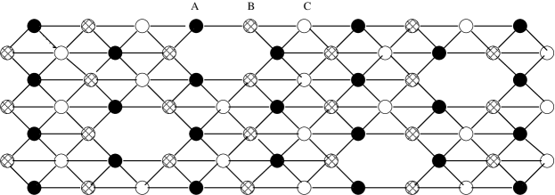
Here $c_{i}$ is a quenched binary variable; $c_{i}=1$ if site $i$ of a $L\times L$ triangular lattice shown in figure (1) is occupied by an Ising spin $s_{i}=\pm{1}$, and $c_{i}=0$ otherwise. Each site has a quenched random-field $h_{i}$ with a Gaussian distribution of mean value zero and standard deviation $\sigma$. The system is placed in a uniform external field $h$ which is varied slowly from $h=-\infty$ to $h=\infty$.

The discrete time, single spin flip serial dynamics of the zero-temperature nonequilibrium RFIM is specified by the equation  glauber ,

$$s_{i}(t+1)=sign\mbox{ }l_{i}(t);l_{i}=J\sum_{j}{c_{j}s_{j}}+h_{i}+h$$ (2)

Figure (1) shows three inter-penetrating sub-lattices A, B and C that comprise a triangular lattice. We randomly dilute the sub-lattice C. Thus only a fraction c of the sites on the sublattice C are occupied by Ising spins. It is easily seen that in the limit $c=0$, the triangular lattice reduces to the honeycomb lattice and the coordination number of the lattice reduces from 6 to 3. For other values of $c$ in the range $0<c<1$, the lattice is characterized by an inhomogeneous coordination number. An occupied site on the sublattice C always has 6 nearest neighbors; 3 on sublattice A and 3 on sublattice B. A site on sublattice A (B) has 3+3$c$ nearest neighbors; 3 on sublattice B (A) and 3c (on average) on sublattice C. Thus the coordination number for an occupied site on C is 6, and the effective coordination number on A or B is given by $z_{eff}($c$)=3(1+$c$)$. The average coordination number when A, B, and C are all taken together is $Z_{av}=6(1+2$c$)/(2+$c$)$. In the following we study the magnetization and the character of the avalanches on the diluted triangular lattice for different values of dilution $c$. The magnetization per site $m(h,\sigma,c;t)$ on the lattice is given by

$$m(h,\sigma,c;t)=\frac{1}{L\times L}\sum_{i}^{L\times L}c_{i}s_{i}$$ (3)

We keep $h$ fixed and iterate the single spin flip dynamics till it reaches a fixed point i.e. a $t$-independent magnetization. We start with $m(h=-\infty,\sigma,c)=-(2+c)/3$ and raise $h$ till some spin becomes unstable and flips up. It may cause some of its neighbors to flip up as well. The dynamics is iterated till a stable configuration is reached. The magnetization of the stable configuration is calculated and the process is repeated by raising $h$ to the next higher value that makes a new site unstable. The number of spins that flip up in going from one fixed point to the next is the size of the avalanche.

The size of an avalanche depends on three quantities; the value of the dilution parameter $c$, the standard deviation $\sigma$ of the quenched random field, and the applied field $h$. For $c=1$  diana there is a critical value of $\sigma=\sigma_{c}(1)$ that separates two different behaviors that are easy to understand qualitatively. For $\sigma>>\sigma_{c}(1)$, the distribution of random-field is very wide. Therefore the spins tend to flip up independently of each other and avalanches are relatively small at any applied field $h$. On the other hand, for $\sigma<<\sigma_{c}(1)$ the distribution of on-site random fields is very narrow. In this case, a single spin flip that changes the local field at each nearest neighbor by an amount $2|J|$ causes a spanning avalanche across the system if the applied field is greater than some threshold. This results in a large change in the magnetization of the system, i.e. a first-order jump in the magnetization at some critical value of the applied field. The size of the jump decreases with increasing $\sigma$ and reduces to zero at the critical point $\sigma=\sigma_{c}(1)$ and $h=h_{c}(1)$. We call it a nonequilibrium critical point because the hysteretic susceptibility of the system diverges at this point. We find that a similar critical point is present on the diluted lattice in the restricted range $0.33<c<1$. The value of $\sigma_{c}(c)$ reduces with decreasing $c$ and drops discontinuously to zero at $c=0.33$ approximately. As mentioned earlier $c=1/3$ corresponds to $z_{eff}=4$. Thus a critical point occurs on the diluted lattice only if $z_{eff}>4$. This is interesting in the context of a similar conclusion reached in the study of the Bethe lattice as well as some other periodic lattices.

The central object of the present study is the determination of $\sigma_{c}(c)$. It seems nearly impossible to determine it analytically. This is not surprising given that exact solutions of Ising models, particularly with quenched disorder, are rare. We have to resort to numerical simulations of the model. Simulations too have difficulties of choosing a good algorithm that suits available computing resources. For each $c$, we first determine a range $\sigma_{min}<\sigma<\sigma_{max}$ that may contain $\sigma_{c}(c)$. This is done by locating $\sigma_{max}$ where no avalanche on the hysteresis loop is macroscopic, and a $\sigma_{min}$ where there is clearly a macroscopic jump in the magnetization. The next step is to study the system for different values of $\sigma$ in the range $[\sigma_{min},\sigma_{max}]$ at suitably chosen intervals $\delta\sigma$ with a view to narrow this range and locate the critical point that separates the two behaviors. There are two difficulties. For each value of $\sigma$, the avalanche distribution is determined by taking an average over a large number of configurations. It is a cpu intensive exercise and a compromise is necessary in choosing an optimal $\delta\sigma$. The size of the step $\delta\sigma$ is one factor that contributes to the error bars in the results. The other difficulty is that fluctuations increase as we approach the vicinity of the critical point. The avalanches that were microscopic for $\sigma>>\sigma_{c}$ grow in size and compete with the avalanches associated with a jump in magnetization even as the jump approaches zero. We need a method to distinguish the infinite avalanche associated with a first order jump in magnetization from an infinite avalanche associated with a critical point. These two categories of avalanches are distinguished from each other by looking at their probability distributions. This is again a cpu intensive process. Qualitatively the largest avalanche associated with a magnetization jump scales linearly with the system size $L$ while the largest avalanche associated with a critical point scales as $L^{1/2}$. The shapes of the avalanche distribution functions for $\sigma<\sigma_{c}$ and $\sigma\approx\sigma_{c}$ are different from each other diana ; farrow . This difference is exploited to pin down $\sigma_{c}$ within error bars as described in the following.

III Simulations

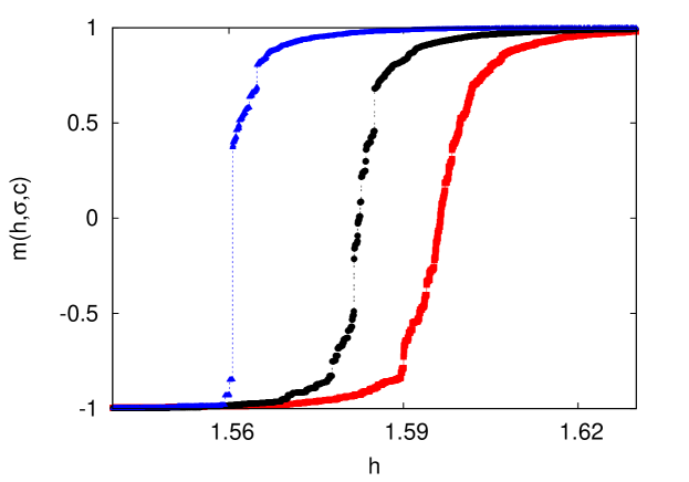
The shape of magnetization curve $m(h,\sigma,c)$ in a changing field $h$ depends on the starting state of the system in addition to $h$, $\sigma$, and $c$. We start from $m(h=-\infty,\sigma,c)=-(2+c)/3$, and raise the field slowly to $h=\infty$. Figure (2) shows $m(h,\sigma,c)$ on a $6000\times 6000$ lattice for $c=0.90$, and three different values of $\sigma=0.95$ (blue triangles), $\sigma=1.01$ (black circles), and $\sigma=1.05$ (red squares) in the range $1.5<h<1.7$. It illustrates three categories of behavior: (i) at smaller values of $\sigma$ (blue triangles) $m(h,\sigma,c)$ has a jump discontinuity, (ii) at larger values of $\sigma$ (red squares) $m(h,\sigma,c)$ looks apparently smooth if we allow for fluctuations due to finite size effects that are naturally present in any numerical simulation, (iii) there is an intermediate region (black circles) where it is relatively difficult to decide if the curve is smooth or has a discontinuity. Somewhere in this region lies a critical value $\sigma_{c}$ with the corresponding magnetization curve being theoretically smooth but containing a point of inflexion at $h=h_{c}$. The inflexion point is the critical point where the fluctuations in the system become anomalously large and consequently the susceptibility of the system diverges. The difficulty is that it is not easy to identify the inflexion point in simulations. Fluctuations also increase with increasing size of the system, and simulated trajectories remain qualitatively similar to the ones shown in figure (2). Thus it is unreasonable to expect that simulation with a larger system (which would anyway require an unreasonably long computer time) would make it any easier to locate the inflexion point by merely looking at the curve. Rather it has to be inferred indirectly from the analysis of fluctuations in its vicinity. The fluctuations are anomalously large not only at the critical point $(h_{c},\sigma_{c})$ but also at the discontinuity in $m(h,\sigma,c)$ at $\sigma<\sigma_{c}$ and $h<h_{c}$. This presents an additional difficulty in determining the critical point. Our approach  farrow ; diana is based on the idea that the character of fluctuations at the critical point is different from the character of fluctuations at a first order discontinuity. The macroscopic discontinuity in magnetization constitutes a large avalanche but avalanches elsewhere on the magnetization trajectory are exponentially small. Thus on a logarithmic scale, the probability $P(s,\sigma,c)$ of an avalanche of size $s$ has two parts, a part that decreases linearly with $s$ and another a delta function peak at $s\approx s_{max}$; $s_{max}$ is of the order of the system size but decreases as $\sigma$ approaches $\sigma_{c}$ from below. Also the distribution of avalanches is asymmetric on the two sides of the discontinuity. Avalanches tend to be larger at the onset of the discontinuity. After the discontinuity has occurred, most of the spins in the system have turned up and the number of potential sites that can turn up reduces drastically. Thus avalanches immediately after a jump in magnetization tend to be smaller in comparison to those just before it. In contrast to this, avalanches on both sides of a critical point are similar to each other. The maximum size of a critical avalanche scales as the square root of the system size while it scales linearly with the system size at a discontinuity. However in spite of these distinguishing features between a first-order and a second order transition, the issue still remains difficult to decide because as $\sigma\rightarrow\sigma_{c}$ from below, the size of the first order jump tends to zero and the Delta function peak at $s=s_{max}$ tends to vanish. In the absence of a more efficient method, we use the same (rather laborious) method to locate critical points on the diluted triangular lattice as was used on the undiluted lattice ($c=1$). In the following we discuss the case $c=0.90$ in detail, and present the results for other values of dilution in the form of a table and graphs.

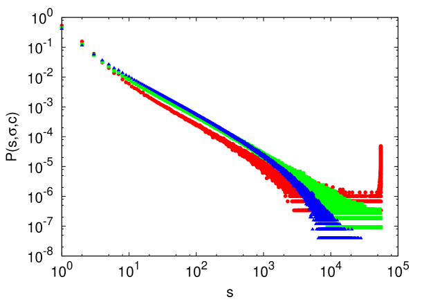
As discussed in reference diana , we count the occurrence of all avalanches of size $s$ as the system is driven from $h=-\infty$ to $\infty$. Let $P(s,\sigma,c)$ be the probability of an avalanche of size $s$ anywhere on the $m(h,\sigma,c)$ curve in an increasing applied field ($h=-\infty$ to $h=\infty$) on a triangular lattice whose sites on sublattice C are occupied with probability $c$. As mentioned earlier, $\log{P(s,\sigma,c)}$ will have a linearly decreasing part in the range $1<s<s_{max}$ if $m(h,\sigma,c)$ has a discontinuity. This is born out by the red (filled circles) curve in figure (3) which shows the raw data for $\sigma=1.1$ on a $240\times 240$ lattice for $c=0.90$ and $50000$ independent realizations of the random-field distribution. The green (filled squares) curve in the same figure shows the data for $\sigma=1.295$ which we estimate to be the critical value. Simulations were performed for several closely spaced values of $\sigma$. However we show the data for only three values of $\sigma$ so as not to crowd figure (3). The data depicted in green is the closest to a linear decrease. The Delta function peak has vanished signifying that the jump in the magnetization has approached zero. Data for $\sigma=1.5$ is shown in blue (filled triangles). We conclude that the value of $\sigma$ corresponding to the blue must be greater than $\sigma_{c}$ due to two reasons: (i) the largest avalanche $s_{max}$ with a non-zero probability of occurrence is far less than the system’s size, and (ii) $P(s,\sigma,c)$ does not approach to zero linearly at $s_{max}$ but rather bends down to it.

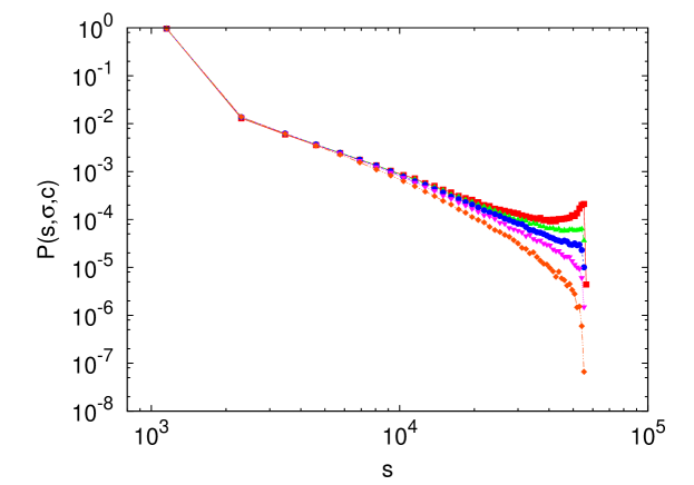
Figure (4) shows similar data as figure (3) but in a binned form. Binning reduces the scatter of the data and we are able to show the data for a larger set of closely spaced $\sigma$ values without crowding the figure too much. The raw data for each value of $\sigma$ has been binned in 50 linear bins. Here the values of $\sigma$ are very close to $\sigma_{c}$ so that the largest avalanche in each case is of the same order of magnitude. What distinguishes different values of $\sigma$ is that curves that bend up near the largest avalanche indicate a tendency to form a Delta function peak. These indicate that the corresponding $\sigma$ is smaller than $\sigma_{c}$. Similarly the curves that bend down near the largest avalanche indicate that the corresponding values of $\sigma$ are larger than $\sigma_{c}$. The curve closest to a straight line (blue circles) belongs to $\sigma_{c}=1.295$. Before closing this section, two comments on the binning procedure may be in order. We have also used logarithmic binning which is normally the preferred binning procedure when the distributions have a fat tail as in our case. This does not change the results presented here. The main purpose of figure (4) is to distinguish between curves that bend up near the end from those that bend down. This is easier for the eye if linear binning is used due to higher density of data points in the region. The second point is that the last bin in each case should be ignored due to lack of sufficient number of data points in this bin.

IV Finite Size Effects and Results

Using the procedure outlined above, we have determined the critical value $\sigma_{c}(L,c)$ on diluted $L\times L$ lattices for various values of $L$ in the range 100 to 600. These are rather small sizes compared with the ones used in the study of the undiluted problem on a square lattice dahmen3 ; spasojevic . However, such small sizes were found to be adequate in reference diana to demonstrate the presence of critical hysteresis on a triangular lattice. In the present study as well, these appear to be adequate to examine the effect of dilution parameter $c$ and the effective coordination number $z_{eff}$ on critical hysteresis in the system. Our results are presented in Table I. According to the scaling hypothesis, the correlation length in the vicinity of the critical point scales as $\sim[\sigma_{c}(c)-\sigma]^{-\nu(c)}$ as $\sigma\rightarrow\sigma_{c}(c)$ from below. The argument on $\nu(c)$ indicates that we are open to the possibility that the the critical exponent $\nu$ may depend on the amount of dilution on the lattice. However, as we shall see in the following, this turns out not to be true within the error bars of our analysis. In the present problem, the correlation length is measured by the largest distance that an avalanche travels from its point of origin. On a finite lattice, the farthest distance an avalanche can travel is limited by the size of the lattice. Thus $L\sim[\sigma_{c}(L,c)-\sigma]^{-\nu(c)}$ where $\sigma_{c}(L,c)$ is a lattice-dependent critical value of $\sigma_{c}(c)$. Allowing for a constant of proportionality, we may write spasojevic

$$L^{-\frac{1}{\nu(c)}}=\frac{\sigma_{c}(L,c)-\sigma_{c}(c)}{\sigma_{c}(c)}\mbox{ or }-\frac{1}{\nu(c)}\log_{10}L=\log_{10}\left[\frac{\sigma_{c}(L,c)}{\sigma_{c}(c)}-1\right]$$ (4)

Here the factor $1/\sigma_{c}(c)$ appearing immediately after the first equality sign is a constant of proportionality. A more general constant of proportionality $1/a$ is considered in equation (5).

Table 1: $\sigma_{c}(L,c)$

L	${c=1.00}$	${c=0.90}$	${c=0.80}$	${c=0.70}$	${c=0.60}$	${c=0.50}$	${c=0.40}$	${c=0.34}$
99	1.63 $\pm 0.01$	1.47$\pm 0.01$	1.305$\pm 0.005$	1.125 $\pm 0.005$	0.885$\pm 0.005$	0.665$\pm 0.005$	0.51$\pm 0.01$	0.485$\pm 0.005$
120	1.59 $\pm 0.01$	1.425$\pm 0.005$	1.255$\pm 0.005$	1.065 $\pm 0.005$	0.83$\pm 0.01$	0.62$\pm 0.01$	0.485$\pm 0.005$	0.46$\pm 0.01$
141	1.56 $\pm 0.01$	1.39$\pm 0.01$	1.215$\pm 0.005$	1.02 $\pm 0.01$	0.785$\pm 0.005$	0.585$\pm 0.005$	0.465$\pm 0.005$	0.44$\pm 0.01$
168	1.525 $\pm 0.005$	1.355$\pm 0.005$	1.175$\pm 0.005$	0.98 $\pm 0.01$	0.745$\pm 0.005$	0.555$\pm 0.005$	0.445$\pm 0.005$	0.425$\pm 0.005$
198	1.50$\pm 0.01$	1.325$\pm 0.005$	1.14$\pm 0.01$	0.94$\pm 0.01$	0.71$\pm 0.01$	0.525$\pm 0.005$	0.425$\pm 0.005$	0.405$\pm 0.005$
240	1.47$\pm 0.01$	1.295 $\pm 0.005$	1.105$\pm 0.005$	0.90$\pm 0.01$	0.675$\pm 0.005$	0.495$\pm 0.005$	0.41$\pm 0.01$	0.39$\pm 0.01$
300	1.44$\pm 0.01$	1.26$\pm 0.01$	1.065$\pm 0.005$	0.86$\pm 0.01$	0.635$\pm 0.005$	0.465$\pm 0.005$	0.39$\pm 0.01$	0.375$\pm 0.005$
360	1.42$\pm 0.01$	1.235$\pm 0.005$	1.04$\pm 0.01$	0.83$\pm 0.01$	0.605$\pm 0.005$	0.445$\pm 0.005$	0.375$\pm 0.005$	0.365$\pm 0.005$
390	1.41$\pm 0.01$	1.225$\pm 0.005$	1.03$\pm 0.01$	0.815$\pm 0.005$	0.595$\pm 0.005$	0.435$\pm 0.005$	0.37$\pm 0.01$	0.36$\pm 0.01$
480	1.39$\pm 0.01$	1.20$\pm 0.01$	1.00$\pm 0.01$	0.785$\pm 0.005$	0.565$\pm 0.005$	0.415$\pm 0.005$	0.355$\pm 0.005$	0.345$\pm 0.005$
600	1.37$\pm 0.01$	1.18$\pm 0.01$	0.975$\pm 0.005$	0.76$\pm 0.01$	0.54$\pm 0.01$	0.395 $\pm 0.005$	0.345$\pm 0.005$	0.335$\pm 0.005$

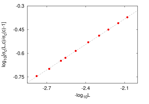
For each value of dilution $c$, the data in Table I is used to plot $-\log_{10}L$ vs. $\log_{10}[\sigma_{c}(L,c)/\sigma_{c}(c)-1]$ for different values of parameter $\sigma_{c}(c)$. The shape of the plot changes from concave up to a straight line, and then to concave down as $\sigma_{c}(c)$ is increased from zero. We search for the best value of the $\sigma_{c}(c)$ that produces a straight line. However, the transition from concave up to concave down is not sharp and spreads over a broad range. This creates a relatively large uncertainty in the value of $\sigma_{c}(c)$ that produces the best fit, and also an uncertainty in the slope of the line. For example, the best fit to a straight line for the data in the second column ($c=0.90$) is obtained for $\sigma_{c}=1.00\pm 0.04$. This is shown in figure (5). The slope of the straight line is equal to $1/\nu(c)=0.54\pm 0.07$, or $\nu(c)=1.85\pm 0.26$. Similarly, we determine $\nu(c)$ for other values of dilution $c$. Our results for $\sigma_{c}(c)$ and $\nu(c)$ for different values of dilution on the triangular lattice are summarized in the following table.

Table 2: $\sigma_{c}(c)$ and $\nu(c)$ for different values of dilution $c$

	${c=1.00}$	${c=0.90}$	${c=0.80}$	${c=0.70}$	${c=0.60}$	${c=0.50}$	${c=0.40}$	${c=0.34}$
$\sigma_{c}$	1.22${\pm 0.04}$	1.00${\pm 0.04}$	0.77${\pm 0.05}$	0.54${\pm 0.05}$	0.33${\pm 0.05}$	0.26${\pm 0.04}$	0.25${\pm 0.03}$	0.25${\pm 0.03}$
$\nu(c)$	1.78${\pm 0.29}$	1.85${\pm 0.26}$	1.87${\pm 0.29}$	1.83${\pm 0.26}$	1.85${\pm 0.28}$	1.64${\pm 0.28}$	1.76${\pm 0.35}$	1.79${\pm 0.33}$

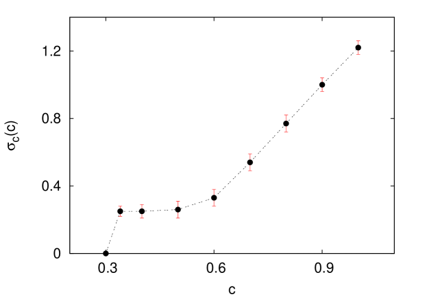
Our simulations reveal a critical value $c_{c}$ of the dilution parameter; $c_{c}=0.33$ approximately. At $c=c_{c}$, $\sigma_{c}(c)$ drops to zero abruptly, and remains zero for $c<c_{c}$ as shown in Figure (6). There is no first order jump in $m(h,\sigma,c)$ for $c<c_{c}$. We have verified this directly from the simulations as well as inferred it from the following. For $c<0.33$, the plot $-\log_{10}L$ vs. $\log_{10}[\sigma_{c}(L,c)/\sigma_{c}(c)-1]$ is never concave up for any $\sigma_{c}(c)>0$. This indicates the absence of a disorder driven jump in the magnetization and therefore the disappearance of a critical point if $c<0.33$. To further validate this point, we also tried as in ref diana , the scaling form

$$L^{-\frac{1}{\nu(c)}}=\frac{\sigma_{c}(L,c)-\sigma_{c}(c)}{a},$$ (5)

where $a$ is an arbitrary parameter. The role of $a$ is to shift the curve along the $y$-axis without changing its shape. If we set $\sigma_{c}(c)=0$ in the above equation, we find that the plot is always concave up for any value of $c>c_{c}$. This means that for $c>c_{c}$, the system possesses a critical point with $\sigma_{c}>0$. On the other hand, for $c<c_{c}$, the curve is a straight line indicating the absence of a critical point.

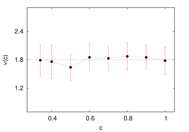
The variation of $\sigma_{c}(c)$ vs. $c$ has been plotted in figures (6), and $\nu(c)$ vs $c$ in figure (7). We may draw the following conclusions from these figures. As the lattice is diluted increasingly, it continues to support a critical point but the value of $\sigma_{c}(c)$ decreases. This is intuitively reasonable because the random dilution of the lattice amounts to a positional disorder in the system that supplements to the disorder due to the random-field. Thus the critical point on the diluted lattice corresponds to a narrower distribution of the random-field as compared with the undiluted case. We also note that the critical dilution $c_{c}=0.33$ corresponds to $z_{eff}\approx 4$.

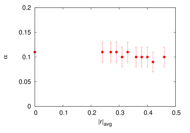
Figure (7) shows that the exponent $\nu(c)$ is independent of $c$ within the error bars. We may expect this universality to hold for other exponents as well because of the relationship between different exponents. It is unlikely that only one exponent in an equation is universal while others are not. We have tried to extract a bit more information from our numerical data regarding other exponents. We have tried the collapse of the integrated avalanche size distribution with the following scaling form  perkovic2 ; dahmen3 :

$$P(S,\sigma)\sim S^{-(\tau+\alpha\beta\delta)}\tilde{P}(S|r|^{1/\alpha})$$ (6)

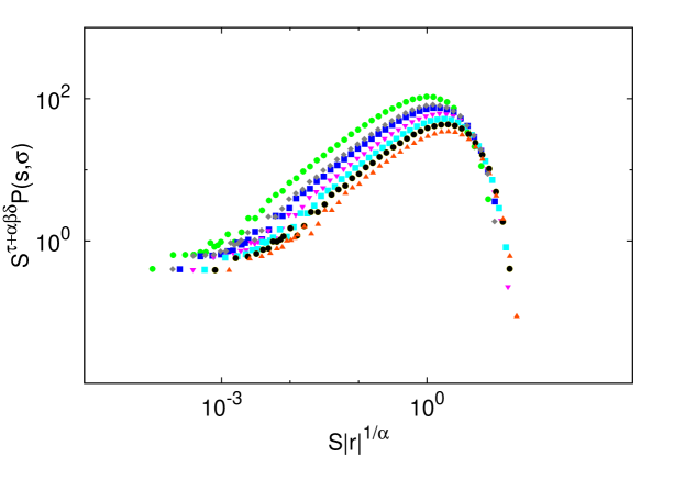
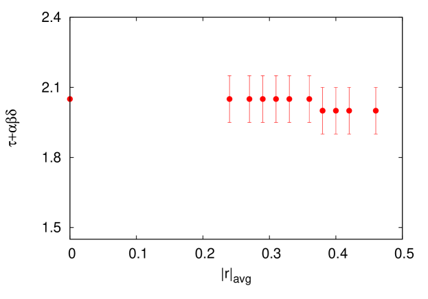
Here $\alpha$ is the exponent describing the largest cut-off avalanche i.e. $S_{max}\sim|r|^{-1/\alpha}$ where $r=\frac{\sigma-\sigma_{c}}{\sigma}$, $\tau$ is the avalanche size exponent, $\beta$ gives the scaling of the change in magnetisation due to spanning avalanche, $\Delta m\sim|r|^{\beta}$, at the critical field. The exponent $\delta$ describes the scaling of the reduced magnetisation with reduced magnetic field, $m\sim h^{\delta}$ at $\sigma_{c}$. Thus the product $P(S,\sigma)\times S^{(\tau+\alpha\beta\delta)}$ is a function of a single variable $S|r|^{1/\alpha}$. Fig(8) shows $\tilde{P}(S|r|^{1/\alpha})$ vs. $S|r|^{1/\alpha}$ for $c=0.80$; $L=168,240$ and $390$; and different values of $\sigma$ ranging from $1.15$ to $1.40$. The curves collapse on each other reasonably well if we choose $\tau+\alpha\beta\delta=2.05$ and $\alpha=0.12$.

We have also examined how the exponents extracted from the collapsing curves depend on $L$ and $|r|$. For this purpose, we fix $c$ and $L$ (say $c=0.80$, and $L=390$), and choose three closely spaced values of $\sigma$ (say $\sigma=1.05,1.06,$ and $1.07$). The three values of $\sigma$ correspond to three closely spaced values of $|r|$. Let $|r|_{avg}$ denotes the average of the three $|r|$ values. We search for the values of $\tau+\alpha\beta\delta$ and $\alpha$ that produce the best collapse of the three curves associated with $|r|_{avg}$. Next we choose several different triplets of closely spaced $\sigma$ values and determine the exponents over a range of values of $|r|_{avg}$. This exercise is repeated for systems of different sizes ($L=168,240,390,600$), and for a range of values of $c$ in the range $c>0.33$. The results for $c=0.80$ are shown in figures (9) and (10) along with the range of variations (error bars) in the values of the exponents. These figures also show the extrapolated values of the exponents in the limit $|r|_{avg}\rightarrow 0$ or $L\rightarrow\infty$. Thus we obtain $\tau+\alpha\beta\delta=2.05\pm 0.05$ and $\alpha=0.11\pm 0.02$ for $c=0.80$. We have checked that the values of the exponents for other values of dilution $c$ lie in the same range as for $c=0.80$. This leads us to conclude that the values of the exponents $\tau+\alpha\beta\delta$ and $\alpha$ are independent of $c$ if $c>0.33$.

V Discussion

We have investigated critical hysteresis on a two dimensional lattice with a variable coordination number. We had to study the problem numerically because exact analytical solutions of this problem are not possible. Simulations of the model suggest that the three parameters of the model $c$, $h$, and $\sigma$ are characterized by critical values $c_{c}$, $h_{c}$, and $\sigma_{c}$ respectively. If $c>c_{c}$, the critical point $(h_{c},\sigma_{c})$ is marked by a diverging avalanche and a critical exponent $\nu(c)$. Within numerical errors, we find that the exponent $\nu$ does not depend on $c$. The critical value $c_{c}$ is approximately equal to $c_{c}=1/3$ which corresponds to $z_{eff}=4$ and $Z_{av}=30/7$. We note that each site on A or B sublattice has three nearest neighbor sites on the C sublattice which are occupied independently with probability $c$. Therefore if $c<1/3$, the probability of a spanning path on A+B through occupied sites on C goes to zero. In this case the C sublattice does not contribute to a diverging correlation length. The cooperative behavior of the system is qualitatively the same as on the honeycomb lattice comprising A and B, and the relevant parameter is $z_{eff}$ rather than $Z_{av}$.

We note that $c=1/3$ corresponds to an effective coordination number $z_{eff}=4$. Thus our results suggest that critical behavior disappears when the coordination number of the lattice drops below four. A similar result holds for the Bethe lattice dhar and also some periodic lattices sabhapandit1 . On the Bethe lattice, the problem can be solved analytically and therefore the mathematical reason for the absence of critical behavior on Bethe lattice of coordination number less than four is understood. However the physical reason for this behavior on periodic lattices is not well understood. It is curious that the lower critical coordination number is also equal to four on the diluted triangular lattice. We could not have anticipated this result beforehand. Our numerical results only suggest $z_{eff}$ to be approximately four within errors but the probabilistic argument mentioned above indicates that it may be exactly equal to four. Thus all the extant results indicate that nonequilibrium critical behavior occurs only on lattices with coordination number equal to four or more irrespective of the dimensionality of the lattice.

Before closing, we wish to comment on the small difference between results presented here for the case $c=1$, and those in reference (16). We find $\sigma_{c}=1.22\pm 0.04$ and $\nu=1.78\pm 0.29$ (for c=1.00) while the values reported in reference (16) are $\sigma_{c}=1.27$ and $\nu=1.6\pm 0.2$. The results are consistent with each other within error bars. As authors of reference (16) are also coauthors of the present paper, we can point out the reason for the difference in the two sets of results. We estimate $\sigma_{c}$ as the best value of this parameter that results in a straight line when the left-hand-side of equation (4) is plotted against its right-hand-side. As explained in the previous section, the range of values of $\sigma_{c}(c)$ that produces an apparent straight line is rather broad. The results in reference (16) rely on a visual scrutiny of the plots and choosing the fit that looks best to the eye. This is of course susceptible to human error. In the present study, we have used the linear least squares fitting technique. It has the convenience of a mechanical method to handle the data contained in Table I but it also has the disadvantage that outlying points have a disproportionate effect on the fit. This contributes to the uncertainty in $\sigma_{c}(c)$ and $\nu$ which is determined by the slope of the straight line. The uncertainties in our results are relatively large for the effort put in this study. This seems unavoidable with the present method. The remark on the closeness of the exponent $\nu$ on the triangular lattice  diana and the simple cubic lattice  perkovic2 should also be taken in the same vein. At a qualitative level, it does suggest that the avalanche-driven exponent may depend on the coordination number rather than the dimensionality of the lattice. However, it is difficult to reach a stronger conclusion with the error bars in our analysis. We hope the present study will motivate further studies of the issues raised here with new and improved techniques.

Figure 1: Triangular lattice with sublattices $A$(black circles), $B$ (shaded circles) and $C$(white circles). $C$ is randomly diluted.

Figure 2: (color online) Magnetization curves on a $6000\times 6000$ diluted triangular lattice with ${c=0.90}$ and for $\sigma=0.95$(blue triangles), $\sigma=1.01$(black circles), and $\sigma=1.05$(red squares).

Figure 3: (color online) Distribution of avalanches $P(s,\sigma,c)$ on a $L\times L$ lattice for $L=240$ and $c=0.90$; $\sigma=1.10$ (red circles with a peak at $s\approx L\times L$), $\sigma=1.295$ (green squares, note the peak at $s\approx L\times L$ has vanished and the plot is almost linear) and $\sigma=1.50$ (blue triangles, the bending of the curve indicates the largest avalanche is smaller than $L\times L$).

Figure 4: (color online) $P(s,\sigma,c)$ for $c=0.90$ and $L=240$ using linear binning; $\sigma=1.25$(red squares), $\sigma=1.27$(green triangles), $\sigma=1.295$(blue circles), $\sigma=1.31$(pink inverted triangles), and $\sigma=1.35$(brown diamonds). Figure shows $\sigma_{c}(L,c)\approx 1.295$ because the corresponding curve is nearly linear; the curves for $\sigma<\sigma_{c}(L,c)$ tend to peak at the largest avalanche while those for $\sigma>\sigma_{c}(L,c)$ tend to bend down.

Figure 5: (color online) Plot of log${}_{10}[\frac{\sigma_{c}(L,c)}{\sigma_{c}(c)}-1]$ vs. -log₁₀ $L$ for $c=0.90$. The best fit to a straight line is obtained for $\sigma_{c}(c)=1.00\pm 0.04$. The slope of the straight line yields $\nu(c)=1.85\pm 0.26$.

Figure 6: (color online) Variation of $\sigma_{c}(c)$ with $c$. The figure shows the absence of critical hysteresis if $c<0.33$.

Figure 7: (color online) Variation of the exponent $\nu(c)$ with $c$; $\nu(c)\approx 1.8\pm 0.3$ for $c>0.33$

Figure 8: (color online) Scaling collapse of the integrated avalanche size distribution for $c=0.80$; $L=168,240,$ and $390$ for seven values of $\sigma$ chosen from the range $1.15-1.40$. The best collapse is obtained for $\tau+\alpha\beta\delta=2.05$ and $\alpha=0.12$.

Figure 9: (color online) Plot of $\tau+\alpha\beta\delta$ vs. $|r|_{avg}$ for $c=0.80$. The values of the exponent are extracted from the best collapse of the avalanche size distribution for each set of three $\sigma$ values ranging from $\sigma=1.00-1.44$ and different values of $L=168,240,390$ and $600$. The extrapolated value is the point at $|r|_{avg}\rightarrow 0$.

Figure 10: (color online) Variation of the exponent $\alpha$ with $|r|_{avg}$ based on the same data and procedure as used to obtain figure (9).

References

- (1) Eduard Vives, J Ortin, L Manosa, I Rafols, Ramon, Antoni, Phys Rev Lett 72, 1694 (1994).
- (2) K.L.Babcock, R.M Westervelt, Phys Rev Lett 64, 2168 (1990); X.che, H. Suhl Phys Rev Lett 64, 1670 (1990).
- (3) M.Bretz, J.B.Cunningham, P.L Karcynski and F.Nori, Phys Rev Lett 69, 2431(1992).
- (4) L.V Meisel, P.J Cote, Phys Rev B 46, 10822(1992).
- (5) J.S Urbach, R.C Madison, J.T Markert, Phys Rev Lett 75, 276(1995).
- (6) J P Sethna, K A Dahmen, S Kartha, J A Krumhansl, B W Roberts, and J D Shore, Phys Rev Lett 70, 3347 (1993);
- (7) O Perkovic, K Dahmen, and J P Sethna, Phys Rev Lett 75, 4528 (1995).
- (8) K Dahmen and J P Sethna, Phys Rev Lett 71, 3222(1993)
- (9) K A Dahmen and J P Sethna, Phys Rev B 53, 14872 (1996).
- (10) O Percovic, K.A Dahmen and J.P Sethna, Phys. Rev. B 59, 6106(1999)
- (11) C Frontera and E Vives, Phys Rev E59, R1295 (1999); Phys Rev E62, 7470 (2000).
- (12) O Percovic,K A Dahmen and J P Sethna, arXiv:cond-mat/9609072 v1
- (13) D.Spasojevic, S. Janicevic and M.Knezevic, Phys. Rev. Lett, 106,175701(2011); Phys Rev E84, 051119 (2011).
- (14) D Dhar, P Shukla, and J P Sethna, J Phys A30, 5259 (1997).
- (15) S Sabhapandit, D Dhar, and P Shukla, Phys Rev Lett 88, 197202 (2002).
- (16) D Thongjaomayum and P.Shukla, Phys Rev E 88, 042138 (2013).
- (17) R J Glauber, J Math Phys 4, 294 (1963).
- (18) C. L. Farrow, P. Shukla, and P. M. Duxbury, J. Phys. A: Math. Theor. 40, F581 (2007); P. Shukla, Pramana 71, 319 (2008).