Spontaneous symmetry breaking in a spin-orbit coupled $f=2$ spinor condensate

Abstract

We study the ground-state density profile of a spin-orbit coupled $f=2$ spinor condensate in a quasi-one-dimensional trap. The Hamiltonian of the system is invariant under time reversal but not under parity. We identify different parity- and time-reversal-symmetry-breaking states. The time-reversal-symmetry breaking is possible for degenerate states. A phase separation among densities of different components is possible in the domain of time-reversal-symmetry breaking. Different types of parity- and time-reversal-symmetry-breaking states are predicted analytically and studied numerically. We employ numerical and approximate analytic solutions of a mean-field model in this investigation to illustrate our findings.

I Introduction

Since the first experimental realization of the spinor Bose-Einstein condensate (BEC) with a gas of ²³Na atoms trapped in an optical trap Stamper-Kurn , a lot of theoretical and experimental studies have been done on these systems ueda ; kurn-ueda . On the theoretical front, mean-field theories have been developed both for $f=1$ Ohmi ; Ho and $f=2$ spinor Bose-Einstein condensates (BECs) Koashi ; Ciobanu . In our previous work sandeep , we studied the ground state structure of an $f=1$ spin-orbit (SO) coupled spinor BEC with fixed magnetization in a quasi-one-dimensional (quasi-1D) trap luca within the framework of the mean-field theory. In the present work, we extend this study to study an SO coupled $f=2$ spinor condensate in a quasi-1D trap. The SO coupling, which relies on the generation of the non-Abelian gauge potentials coupling the neutral atoms Osterloh , can be experimentally realized by controlling the atom-light interaction. A variety of SO couplings can be engineered by Raman dressing the hyper-fine states. The parameters of atom-light interaction Hamiltonian, and hence those of coupling can be controlled independently young . The SO interaction with equal strengths of Rashba Bychkov and Dresselhaus Dresselhaus ; Liu couplings has been achieved recently Lin ; Linx . The experimentalists employed a pair of Raman lasers to create a momentum-sensitive coupling between two internal atomic states of ⁸⁷Rb Lin ; Linx . This has lead to a flurry of other experiments on SO-coupled pseudo-spinor BECs JY_Zhang . The generation of SO coupling involving the three hyper-fine spin components of an $f=1$ spinor condensate using Raman dressing has also been studied theoretically Juzeliunas ; lan . Recently, SO coupling has also been experimentally realized in degenerate Fermi gases of ⁴⁰K and ⁶Li P_Wang .

Wang et al. Wang studied theoretically the ground states of pseudo-spin-$1/2$ two-component BEC with SO coupling and of three-component $f=1$ spinor BEC. In the presence of SO coupling, the ground states of all spinor BECs $-$ pseudo-spin-$1/2$ Gopalakrishnan , $f=1$ Ruokokoski , and $2$ Kawakami may exhibit different types of nontrivial density distribution. In the presence of a uniform magnetic field the ground states of $f=1$ Ohmi ; Ho ; Zhou ; Matuszewski and $f=2$ Ciobanu ; ueda ; GP-Zheng spinor BECs exhibit interesting behavior including the possibility of a phase separation Matuszewski ; Lin among different spin components. There have also been different static and dynamic studies in SO-coupled BECs, such as, Josephson oscillation josep , intrinsic spin-Hall effect Larson , solitons sol , force on a moving impurity He , chiral confinement Merkl , and superfluidity super , etc.

In this paper, we investigate the ground state of an SO-coupled $f=2$ spinor BEC in a quasi-1D trap for an arbitrary magnetization. The Hamiltonian of this system is invariant under time reversal $\cal T$ but not under parity. Consequently, different types of parity-breaking states are found. Time-reversal symmetry-breaking states are also found in the presence of degeneracy. In the absence of degeneracy, the states preserve time-reversal symmetry. The five spin-component wave functions of the $f=2$ spinor condensate satisfy a coupled mean-field Gross-Pitaevskii (GP) equation with three interaction parameters: $c_{0}\propto(4a_{2}+3a_{4})/7$, $c_{1}\propto(a_{4}-a_{2})/7$, and $c_{2}\propto(7a_{0}-10a_{2}+3a_{4})/7$, where $a_{0},~{}a_{2}$, and $a_{4}$ are the $s$-wave scattering lengths in total spin $f_{\rm tot}=0,2$ and $4$ channels. The whole $c_{1}$ versus $c_{2}$ parameter space can be divided into sub spaces with distinct symmetry properties of the densities of spinor components. We have the ferromagnetic phase for $c_{1}<0$ and $c_{2}>20c_{1}$, anti-ferromagnetic phase for $c_{2}<0$ and $c_{2}<20c_{1}$, and cyclic phase for $c_{1}>0$ and $c_{2}>0$. In the ferromagnetic phase increasing magnetization lowers energy, whereas in the anti-ferromagnetic phase the lowest energy is attained for zero magnetization. Miscible configuration for five component densities of an SO-coupled spinor BEC is obtained for $c_{2}<20c_{1}$ and a phase separation is possible for $c_{2}>20c_{1}$. We find that for sufficiently strong spin-orbit coupling, the SO-coupled spinor condensate has atoms only in $m_{f}=2$ and $m_{f}=-2$ states. Time-reversal-symmetry is preserved for states only in the anti-ferromagnetic phase, and can be broken in other phases. As parity is not a good quantum number, it is broken in all domains. We use the numerical solution of the generalized mean-field GP equation H_Wang for this investigation.

The paper is organized as follows. In Sec. II, we describe the coupled GP equations used to study the SO-coupled $f=2$ spinor BEC in a quasi-1D trap. From an analytic consideration of energy minimization, we predict the expected density profiles for different set of parameters. Specifically, we predict the parameter space, where a phase separation can take place. We also predict different types of parity-breaking states. In Sec. III, we numerically study the SO-coupled spinor BEC in a quasi-1D trap. We identify the different types of symmetry-breaking states and phase-separated states in different parameter domains. We conclude by providing a summary of this study in Sec. IV.

II Mean-field model for a SO-coupled BEC

Spin-orbit coupling can be generated for the hyper-fine states of neutral atoms by suitably controlling the atom-light interaction. The idea was realized experimentally by Lin et al. Lin for two hyper-spin components of the ⁸⁷Rb hyper-fine state 5S_1/2 employing two counter-propagating Raman lasers of wavelength $\lambda_{r}$ oriented at an angle $\beta_{r}$. This lead to the SO coupling with strength $\gamma=\hbar k_{r}/m$, where $k_{r}=2\pi\sin(\beta_{r}/2)/\lambda_{r}$ and $m$ is the mass of an atom. However, here we consider the SO coupling among the five spin components of the $f=2$ state, e.g., $|f=2,m_{f}=2\rangle$, $|f=2,m_{f}=1\rangle$, $|f=2,m_{f}=0\rangle$, $|f=2,m_{f}=-1\rangle$ and $|f=2,m_{f}=-2\rangle$, where $m_{f}$ is the $z$ projection of $f$. By generalizing the method discussed in Ref. lan , this SO coupling among the five hyper-fine spin components can be generated by engineering a suitable atom-light interaction Hamiltonian as in Ref. Lin .

In order to realize a quasi-1D SO-coupled spin-2 BEC along $x$ axis, we consider a trapping potential with angular frequencies along $y$ and $z$ axes much larger than that along $x$ axis. The resultant strong transverse confinement ensures that the dynamics is frozen along $y$ and $z$ axes. Then, the single-particle quasi-1D Hamiltonian of the system under the action of a strong transverse trap of angular frequencies $\omega_{y}$ and $\omega_{z}$ along $y$ and $z$ axes, respectively, can be written as Lin ; Y_Zhang

$$H_{0}=\frac{p_{x}^{2}}{2m}+\gamma p_{x}\Sigma_{z}+\Omega\Sigma_{x},$$ (1)

where $p_{x}=-i\hbar\partial_{x}$ is the momentum operator along $x$ axis, $\Omega$ is the Rabi frequency Lin ; Linx , and $\Sigma_{z}$ and $\Sigma_{x}$ are the irreducible representations of the $z$ and $x$ components of the spin-$2$ matrix, and are given by

$$\Sigma_{z}=\left(\begin{array}[]{ccccc}2&0&0&0&0\\ 0&1&0&0&0\\ 0&0&0&0&0\\ 0&0&0&-1&0\\ 0&0&0&0&-2\end{array}\right),$$ (7)

$$\Sigma_{x}=\left(\begin{array}[]{ccccc}0&1&0&0&0\\ 1&0&\sqrt{\frac{3}{2}}&0&0\\ 0&\sqrt{\frac{3}{2}}&0&\sqrt{\frac{3}{2}}&0\\ 0&0&\sqrt{\frac{3}{2}}&0&1\\ 0&0&0&1&0\end{array}\right).$$ (13)

II.1 Mean-field model in a quasi-1D trap

If the interactions among the atoms in the BEC are taken into account, in the Hartree approximation, using the single particle model Hamiltonian (1), a quasi-1D luca spin-2 BEC can be described by the following set of five coupled mean-field partial differential GP equations for the wave-function components $\psi_{j}$ ueda ; H_Wang

$$i\hbar \frac{\partial\psi_{2}}{\partial t}=\left(-\frac{\hbar^{2}}{2m}\frac{\partial^{2}}{\partial x^{2}}+V(x)+c_{0}\rho\right)\psi_{2}-2i\hbar\gamma\frac{\partial\psi_{2}}{\partial x}$$

$$+c_{1}\big{(}F_{-}\psi_{1}+2F_{z}\psi_{2}\big{)}+\big{(}{c_{2}}/{\sqrt{5}}\big{)}\Theta\psi_{-2}^{*}+\Omega\psi_{1},$$ (14)

$$i\hbar \frac{\partial\psi_{1}}{\partial t}=\left(-\frac{\hbar^{2}}{2m}\frac{\partial^{2}}{\partial x^{2}}+V(x)+c_{0}\rho\right)\psi_{1}-i\hbar\gamma\frac{\partial\psi_{1}}{\partial x}$$

$$+c_{1}\big{(}\sqrt{3/2}F_{-}\psi_{0}+F_{+}\psi_{2}+F_{z}\psi_{1}\big{)}-\big{(}{c_{2}}/\sqrt{5}\big{)}\Theta\psi_{-1}^{*}$$

$$+\Omega\big{[}\psi_{2}+\big{(}\sqrt{3}/2\big{)}\psi_{0}\big{]},$$ (15)

$$i\hbar \frac{\partial\psi_{0}}{\partial t}=\left(-\frac{\hbar^{2}}{2m}\frac{\partial^{2}}{\partial x^{2}}+V(x)+c_{0}\rho\right)\psi_{0}+\frac{c_{2}}{\sqrt{5}}\Theta\psi_{0}^{*}$$

$$+\frac{\sqrt{6}}{2}c_{1}\big{(}F_{-}\psi_{-1}+F_{+}\psi_{1}\big{)}+\frac{\sqrt{3}}{2}\Omega\big{(}\psi_{1}+\psi_{-1}\big{)},$$ (16)

$$i\hbar \frac{\partial\psi_{-1}}{\partial t}=\left(-\frac{\hbar^{2}}{2m}\frac{\partial^{2}}{\partial x^{2}}+V(x)+c_{0}\rho\right)\psi_{-1}+i\hbar\gamma\frac{\partial\psi_{-1}}{\partial x}$$

$$+c_{1}\big{(}\sqrt{3/2}F_{+}\psi_{0}+F_{-}\psi_{-2}-F_{z}\psi_{-1}\big{)}-\big{(}c_{2}/\sqrt{5}\big{)}\Theta\psi_{1}^{*}$$

$$+\Omega\big{[}\big{(}{\sqrt{3}}/{2}\big{)}\psi_{0}+\psi_{-2}\big{]},$$ (17)

$$i\hbar \frac{\partial\psi_{-2}}{\partial t}=\left(-\frac{\hbar^{2}}{2m}\frac{\partial^{2}}{\partial x^{2}}+V(x)+c_{0}\rho\right)\psi_{-2}+2i\hbar\gamma\frac{\partial\psi_{-2}}{\partial x}$$

$$+c_{1}\big{(}F_{+}\psi_{-1}-2F_{z}\psi_{-2}\big{)}+\big{(}c_{2}/\sqrt{5}\big{)}\Theta\psi_{2}^{*}+\Omega\psi_{-1},$$ (18)

where $V(x)=m\omega_{x}^{2}x^{2}/2$ is the 1D harmonic trap, $c_{0}=2\hbar^{2}(4a_{2}+3a_{4})/(7ml_{yz}^{2})$, $c_{1}=2\hbar^{2}(a_{4}-a_{2})/(7ml_{yz}^{2})$, $c_{2}=2\hbar^{2}(7a_{0}-10a_{2}+3a_{4})/(7ml_{yz}^{2})$, $a_{0}$, $a_{2}$ and $a_{4}$ are the $s$-wave scattering lengths in the total spin $f_{\mathrm{tot}}=0,2$ and $4$ channels, respectively, $\rho_{j}=|\psi_{j}|^{2}$ with $j=2,1,0,-1,-2$ are the component densities, $\rho(x)=\sum_{j=-2}^{2}\rho_{j}$ is the total density, and $l_{yz}=\sqrt{\hbar/(m\omega_{yz})}$ with $\omega_{yz}=\sqrt{\omega_{y}\omega_{z}}$ is the oscillator length in the transverse $y-z$ plane and

$$F_{+}=F_{-}^{*} =2(\psi_{2}^{*}\psi_{1}+\psi_{-1}^{*}\psi_{-2})+\sqrt{6}(\psi_{1}^{*}\psi_{0}+\psi_{0}^{*}\psi_{-1}),$$

$$F_{z} =2(|\psi_{2}|^{2}-|\psi_{-2}|^{2})+|\psi_{1}|^{2}-|\psi_{-1}|^{2},$$

$$\Theta =\frac{2\psi_{2}\psi_{-2}-2\psi_{1}\psi_{-1}+\psi_{0}^{2}}{\sqrt{5}}.$$

Here $\mathbf{F}=(F_{x},F_{y},F_{z})$ is the spin density vector; $F_{\pm}=F_{x}\pm F_{y}.$ The normalization condition is $\int_{-\infty}^{\infty}dx\rho(x)=N,$ where $N$ is the total number of atoms. In order to transform Eqs. (14) - (18) into dimensionless form, we use the scaled variables defined as

$$\tilde{t}=\omega_{x}t,~{}\tilde{x}=\frac{x}{l_{0}},~{}\phi_{j}(\tilde{x},\tilde{t})=\frac{\sqrt{l_{0}}}{\sqrt{N}}\psi_{j}(\tilde{x},\tilde{t}),$$ (19)

where $l_{0}=\sqrt{\hbar/(m\omega_{x}}$) is the oscillator length along $x$ axis. Using these dimensionless variables, the coupled mean-field Eqs. (14) - (18) in dimensionless form are

$$i \frac{\partial\phi_{2}}{\partial\tilde{t}}=\left(-\frac{1}{2}\frac{\partial^{2}}{\partial\tilde{x}^{2}}+\tilde{V}+\tilde{c}_{0}\tilde{\rho}\right)\phi_{2}-2i\tilde{\gamma}\frac{\partial\phi_{2}}{\partial\tilde{x}}$$

$$+\tilde{c}_{1}\big{(}\tilde{F}_{-}\phi_{1}+2\tilde{F}_{\tilde{z}}\phi_{2}\big{)}+\big{(}{\tilde{c}_{2}}/{\sqrt{5}}\big{)}\tilde{\Theta}\phi_{-2}^{*}+\tilde{\Omega}\phi_{1},$$ (20)

$$i \frac{\partial\phi_{1}}{\partial\tilde{t}}=\left(-\frac{1}{2}\frac{\partial^{2}}{\partial\tilde{x}^{2}}+\tilde{V}+\tilde{c}_{0}\tilde{\rho}\right)\phi_{1}-i\tilde{\gamma}\frac{\partial\phi_{1}}{\partial\tilde{x}}$$

$$+\tilde{c}_{1}\big{(}\sqrt{3/2}\tilde{F}_{-}\phi_{0}+\tilde{F}_{+}\phi_{2}+\tilde{F}_{\tilde{z}}\phi_{1}\big{)}-\big{(}\tilde{c}_{2}/\sqrt{5}\big{)}\tilde{\Theta}\phi_{-1}^{*}$$

$$+\tilde{\Omega}\big{[}\phi_{2}+\big{(}{\sqrt{3}}/{2}\big{)}\phi_{0}\big{]},$$ (21)

$$i \frac{\partial\phi_{0}}{\partial\tilde{t}}=\left(-\frac{1}{2}\frac{\partial^{2}}{\partial\tilde{x}^{2}}+\tilde{V}+\tilde{c}_{0}\tilde{\rho}\right)\phi_{0}+\frac{\tilde{c}_{2}}{\sqrt{5}}\tilde{\Theta}\phi_{0}^{*}$$

$$+\frac{\sqrt{6}}{2}\tilde{c}_{1}\big{(}\tilde{F}_{-}\phi_{-1}+\tilde{F}_{+}\phi_{1}\big{)}+\frac{\sqrt{3}}{2}\tilde{\Omega}(\phi_{1}+\phi_{-1}),$$ (22)

$$i \frac{\partial\phi_{-1}}{\partial\tilde{t}}=\left(-\frac{1}{2}\frac{\partial^{2}}{\partial\tilde{x}^{2}}+\tilde{V}+\tilde{c}_{0}\tilde{\rho}\right)\phi_{-1}+i\tilde{\gamma}\frac{\partial\phi_{-1}}{\partial\tilde{x}}$$

$$+\tilde{c}_{1}\big{(}{\sqrt{3/2}}\tilde{F}_{+}\phi_{0}+\tilde{F}_{-}\phi_{-2}-\tilde{F}_{\tilde{z}}\phi_{-1}\big{)}-\big{(}{\tilde{c}_{2}}/{\sqrt{5}}\big{)}\tilde{\Theta}\phi_{1}^{*}$$

$$+\tilde{\Omega}\big{[}\big{(}{\sqrt{3}}/{2}\big{)}\phi_{0}+\phi_{-2}\big{]},$$ (23)

$$i \frac{\partial\phi_{-2}}{\partial\tilde{t}}=\left(-\frac{1}{2}\frac{\partial^{2}}{\partial\tilde{x}^{2}}+\tilde{V}+\tilde{c}_{0}\tilde{\rho}\right)\phi_{-2}+2i\tilde{\gamma}\frac{\partial\phi_{-2}}{\partial\tilde{x}}$$

$$+\tilde{c}_{1}\big{(}\tilde{F}_{+}\phi_{-1}-2\tilde{F}_{\tilde{z}}\phi_{-2}\big{)}+\big{(}{\tilde{c}_{2}}/{\sqrt{5}}\big{)}\tilde{\Theta}\phi_{2}^{*}+\tilde{\Omega}\phi_{-1},$$ (24)

where $\tilde{V}=\tilde{x}^{2}/2$, $\tilde{\gamma}=\hbar k_{r}/(m\omega_{x}l_{0})$, $\tilde{\Omega}=\Omega/(\hbar\omega_{x})$, $\tilde{c}_{0}=2N(4a_{2}+3a_{4})/(7l^{2}_{yz})$, $\tilde{c}_{1}=2N(a_{4}-a_{2})/(7l^{2}_{yz})$, $\tilde{c}_{2}=2N(7a_{0}-10a_{2}+3a_{4})/(7l^{2}_{yz})$, $\tilde{\rho}_{j}=|\phi_{j}|^{2}$ with $j=2,1,0,-1,-2$, and $\tilde{\rho}=\sum_{j=-2}^{2}|\phi_{j}|^{2}$ and

$$\tilde{F}_{+}=\tilde{F}_{-}^{*}= 2(\phi_{2}^{*}\phi_{1}+\phi_{-1}^{*}\phi_{-2})+\sqrt{6}(\phi_{1}^{*}\phi_{0}+\phi_{0}^{*}\phi_{-1}),$$

$$\tilde{F}_{\tilde{z}}= 2(|\phi_{2}|^{2}-|\phi_{-2}|^{2})+|\phi_{1}|^{2}-|\phi_{-1}|^{2},$$

$$\tilde{\Theta}= \frac{2\phi_{2}\phi_{-2}-2\phi_{1}\phi_{-1}+\phi_{0}^{2}}{\sqrt{5}}.$$

The normalization condition satisfied by $\phi_{j}$’s is $\int_{-\infty}^{\infty}\tilde{\rho}(\tilde{x})d\tilde{x}=1.$ One of the aims in the present work is to find the ground state of an $f=2$ spinor condensate with a fixed magnetization, which is defined by

$${\cal M}=\int_{-\infty}^{\infty}\tilde{F}_{\tilde{z}}d\tilde{x}.$$ (25)

Depending on the values of $\tilde{c}_{1}$ and $\tilde{c}_{2}$ the system in the absence of magnetic field and SO coupling can have a variety of ground states ueda . For the sake of simplicity of notations, we will represent the dimensionless variables without tilde in the rest of the paper.

II.2 Uniform BEC: Analytic Consideration

The energy of a uniform (trapless) spinor BEC in the presence of SO coupling and magnetic field is ueda ; H_Wang

$$E =N\int_{-\infty}^{\infty}\Big{\{}\frac{1}{2}\sum_{j=-2}^{2}\left|\frac{d\phi_{j}}{dx}\right|^{2}-i\gamma\sum_{j=-2}^{2}j\phi_{j}^{*}\frac{d\phi_{j}}{dx}$$

$$+\big{(}{c_{0}}\rho^{2}+{c_{1}}|\mathbf{F}|^{2}+{c_{2}}|\Theta|^{2}\big{)}/2+\Omega\big{[}\phi_{2}^{*}\phi_{1}+\phi_{1}^{*}\phi_{2}$$

$$+\phi_{-1}^{*}\phi_{-2}+\phi_{-2}^{*}\phi_{-1}+\big{(}{\sqrt{3}}/{2}\big{)}\big{(}\phi_{1}^{*}\phi_{0}+\phi_{0}^{*}\phi_{1}+$$

$$\phi_{0}^{*}\phi_{-1}+\phi_{-1}^{*}\phi_{0}\big{)}\big{]}\Big{\}}dx.$$ (26)

First we consider the formation of spatially-separated non-overlapping (phase-separated) states from a consideration of energy minimization. As in the case of a $f=1$ spinor BEC sandeep , the energy term proportional to $c_{0}$ in Eq. (26) can not lead to a phase separation as it contains terms $Nc_{0}\int(\rho_{j}^{2}/2+\rho_{j}^{\prime 2}/2+\rho_{j}\rho_{j}^{\prime})dx$, where $j,j^{\prime}=2,1,0,−1,-2$ and $j\neq j^{\prime}$, and hence corresponds to a situation where inter- and intra-species interactions are of equal strength. The situation is analogous to a binary BEC with a $a_{12}=\sqrt{a_{11}a_{22}}$ , where $a_{11}$ and $a_{22}$ are intra-species and $a_{12}$ the inter-species scattering lengths. Such a binary BEC has equal strengths of inter- and intra-species nonlinearities and is always miscible in the presence of a 1D harmonic trap Ao ; Gautam . The interaction energy of the $f=2$ spinor condensate in the absence of SO coupling and magnetic field ($\gamma=\Omega=0$) can be written as

$$E_{\rm int}=N\int\Big{\{}\frac{c_{1}}{2}\Big{[}4\rho_{2}^{2}+\rho_{1}^{2}+\rho_{-1}^{2}+4\rho_{-2}^{2}$$

$$+6\rho_{0}(\rho_{1}+\rho_{-1})+8\sqrt{\rho_{1}\rho_{2}\rho_{-1}\rho_{-2}}\cos(\theta_{-1-2}-\theta_{21})$$

$$+12\rho_{0}\sqrt{\rho_{1}\rho_{-1}}\cos(\theta_{0-1}-\theta_{10})+4\sqrt{6}\Big{(}\rho_{-1}\sqrt{\rho_{-2}\rho_{0}}$$

$$\times\cos(\theta_{-1-2}-\theta_{0-1})+\sqrt{\rho_{-1}\rho_{-2}\rho_{0}\rho_{1}}\cos(\theta_{-1-2}-\theta_{10})$$

$$+\sqrt{\rho_{2}\rho_{1}\rho_{0}\rho_{-1}}\cos(\theta_{21}-\theta_{0-1})+\rho_{1}\sqrt{\rho_{2}\rho_{0}}\cos(\theta_{21}-\theta_{10})\Big{)}$$

$$+8\rho_{2}\rho_{1}+8\rho_{-1}\rho_{-2}-4\rho_{2}\rho_{-1}-8\rho_{2}\rho_{-2}-2\rho_{1}\rho_{-1}$$

$$-4\rho_{1}\rho_{-2}\Big{]}+\frac{c_{2}}{10}\Big{[}4\rho_{2}\rho_{-2}+4\rho_{1}\rho_{-1}-8\sqrt{\rho_{2}\rho_{1}\rho_{-2}\rho_{-1}}$$

$$\times\cos(\theta_{21}-\theta_{-1-2})+4\rho_{0}\left(\sqrt{\rho_{2}\rho_{-2}}\cos(\theta_{20}-\theta_{0-2})\right.$$

$$\left.-\sqrt{\rho_{1}\rho_{-1}}\cos(\theta_{10}-\theta_{0-1})\right)+\rho_{0}^{2}\Big{]}\Big{\}}dx,$$ (27)

where the wave-function component $\phi_{j}$ is written as $\phi_{j}=\sqrt{\rho_{j}}\exp(i\theta_{j})$ with $\theta_{j}$ the phase. The phase difference between the $i$th and $j$th components is written as $\theta_{ij}=\theta_{i}-\theta_{j}$.

To understand the phase separation and spontaneous symmetry breaking of the states, we consider the stationary eigenvalue problem of the lowest-energy state of a uniform non-interacting system with SO coupling while Eqs. (20) - (24) become

$$E\phi_{j}(x)=N\left[-\frac{1}{2}\frac{\partial^{2}}{\partial x^{2}}-ij\gamma\frac{\partial}{\partial x}\right]\phi_{j}(x).$$ (28)

The two independent solutions of Eq. (28) for the lowest-energy state are $\phi_{\pm 2}=\alpha_{\pm 2}\exp(\mp 2i\gamma x)$ with normalization $|\alpha_{2}|^{2}+|\alpha_{-2}|^{2}=1$ and $\phi_{\pm 1}=\phi_{\pm 0}=0$ with energy $E\equiv E_{\mathrm{min}}=-2N\gamma^{2}$. The components $j=\pm 1,0$ have higher energies. In the presence of a trap and interactions, in the actual numerical calculation, for a sufficiently large SO coupling $\gamma$ only the components $j=\pm 2$ survive. Hence, the analytic solutions of Eq. (28) is very useful to understand many features of the actual numerical solution. It is clear from Eq. (28) that these plane-wave solutions will lead to smooth density profiles in the presence of a trap while their real and imaginary parts will, in general, have oscillating behavior. In the case, when the two components $j=\pm 2$ survive, the interaction energy (II.2) becomes

$$E_{\rm int}=2N\int\Big{[}c_{1}(\rho_{2}+\rho_{-2})^{2}+\frac{c_{2}-20c_{1}}{5}\rho_{2}\rho_{-2}\Big{]}dx.$$ (29)

In Eq. (29), only the product term $\rho_{2}\rho_{-2}$ controls the phase separation between components $\pm 2$. A repulsive (positive) product term will facilitate a phase separation, as the energy can then be minimized by reducing the overlap between the components. This will happen for $c_{2}>20c_{1}.$

In the presence of SO coupling the Hamiltonian is invariant under time reversal ${\cal T}$ but not under parity. Hence, parity is not a good quantum number. Different types of simple parity-breaking states are found. The non-degenerate states should possess time-reversal symmetry. However, a pair of degenerate states, which transform into each other when operated upon by ${\cal T},$ break time-reversal symmetry. For a sufficiently large $\gamma$, when only the components $j=\pm 2$ survive, the time reversal symmetry is broken for the phase-separated profiles, whereas the miscible profiles preserve time-reversal symmetry. Next we consider different types of symmetry-breaking states.

First we consider different overlapping parity-breaking, nevertheless time-reversal-symmetric, states. The parity property of $\phi_{\pm 2}$ and the relations between the real and imaginary parts, denoted by ${\cal R}$ and ${\cal I}$ respectively, of $\phi_{2}$ and $\phi_{-2}$ for some of these parity-breaking and time-reversal-symmetric states are listed in Table 1.

$\alpha_{2}$	$\alpha_{-2}$	Parity property of $\phi_{\pm 2}$	Relation between $\phi_{2}$ and $\phi_{-2}$
$\frac{\pm 1}{\sqrt{2}}$	$\frac{\pm 1}{\sqrt{2}}$	${\cal R}[\phi_{\pm 2}(x)]={\cal R}[\phi_{\pm 2}(-x)]$, ${\cal I}[\phi_{\pm 2}(x)]=-{\cal I}[\phi_{\pm 2}(-x)]$	${\cal R}[\phi_{2}(x)]={\cal R}[\phi_{-2}(x)],$ ${\cal I}[\phi_{2}(x)]=-{\cal I}[\phi_{-2}(x)]$
$\frac{\pm 1}{\sqrt{2}}$	$\frac{\mp 1}{\sqrt{2}}$	${\cal R}[\phi_{\pm 2}(x)]={\cal R}[\phi_{\pm 2}(-x)],$ ${\cal I}[\phi_{\pm 2}(x)]=-{\cal I}[\phi_{\pm 2}(-x)]$	${\cal R}[\phi_{2}(x)]=-{\cal R}[\phi_{-2}(x)],$ ${\cal I}[\phi_{2}(x)]={\cal I}[\phi_{-2}(x)]$
$\frac{\pm i}{\sqrt{2}}$	$\frac{\pm i}{\sqrt{2}}$	${\cal R}[\phi_{\pm 2}(x)]=-{\cal R}[\phi_{\pm 2}(-x)],$ ${\cal I}[\phi_{\pm 2}(x)]={\cal I}[\phi_{\pm 2}(-x)]$	${\cal R}[\phi_{2}(x)]=-{\cal R}[\phi_{-2}(x)],$ ${\cal I}[\phi_{2}(x)]={\cal I}[\phi_{-2}(x)]$
$\frac{\pm i}{\sqrt{2}}$	$\frac{\mp i}{\sqrt{2}}$	${\cal R}[\phi_{\pm 2}(x)]=-{\cal R}[\phi_{\pm 2}(-x)],$ ${\cal I}[\phi_{\pm 2}(x)]={\cal I}[\phi_{\pm 2}(-x)]$	${\cal R}[\phi_{2}(x)]={\cal R}[\phi_{-2}(x)],$ ${\cal I}[\phi_{2}(x)]=-{\cal I}[\phi_{-2}(x)]$
$\frac{i}{\sqrt{2}}$	$\frac{\pm 1}{\sqrt{2}}$	${\cal R}[\phi_{2}(x)]=-{\cal R}[\phi_{2}(-x)],$ ${\cal R}[\phi_{-2}(x)]={\cal R}[\phi_{-2}(-x)],$ ${\cal I}[\phi_{2}(x)]={\cal I}[\phi_{2}(-x)],$ ${\cal I}[\phi_{-2}(x)]=-{\cal I}[\phi_{-2}(-x)]$	${\cal R}[\phi_{2}(x)]=\pm{\cal I}[\phi_{-2}(x)],$ ${\cal I}[\phi_{2}(x)]=\pm{\cal R}[\phi_{-2}(x)]$
$\frac{\pm 1}{\sqrt{2}}$	$\frac{i}{\sqrt{2}}$	${\cal R}[\phi_{2}(x)]={\cal R}[\phi_{2}(-x)],$ ${\cal R}[\phi_{-2}(x)]=-{\cal R}[\phi_{-2}(-x)],$ ${\cal I}[\phi_{2}(x)]=-{\cal I}[\phi_{2}(-x)],$ ${\cal I}[\phi_{-2}(x)]={\cal I}[\phi_{-2}(-x)]$	${\cal R}[\phi_{2}(x)]=\pm{\cal I}[\phi_{-2}(x)],$ ${\cal I}[\phi_{2}(x)]=\pm{\cal R}[\phi_{-2}(x)]$

Table 1: Parity-breaking states with different choices of $\alpha_{\pm 2}$. The third column defines the parity of the real and imaginary parts of $\phi_{\pm 2}$, whereas the fourth column shows the relations between the real and imaginary parts of $\phi_{2}$ and $\phi_{-2}$.

In these examples the real and imaginary parts of the wave function may have definite parity, but not the total wave function, as parity is not a good quantum number. However, no such simple relation is obtained for a general $\alpha_{\pm 2}$, where neither the real part nor the imaginary part of the wave-function components have a definite parity. Also, similar symmetry-breaking states are expected for the $j=\pm 1$ component states when they are nonzero. These types of symmetry-breaking states were found in the actual numerical calculation in the presence of trap and interaction terms.

Now we consider some examples of time-reversal symmetry-breaking states in the presence of SO coupling. These states are phase-separated (non-overlapping). There could be a complete phase separation between the $j=\pm 2$ components when the two components symmetrically move to two sides of $x=0$. In that case, suppose the components $j=\pm 2$ are centered at $x=\pm x_{0}$, then there will be no definite parity of the real and imaginary parts, but one can have properties, such as, ${\cal R}[\phi_{2}(x-x_{0})]=\pm{\cal R}[\phi_{-2}(x+x_{0})]$, ${\cal I}[\phi_{2}(x-x_{0})]=\mp{\cal I}[\phi_{-2}(x+x_{0})]$, or ${\cal R}[\phi_{2}(x-x_{0})]=\pm{\cal I}[\phi_{-2}(x+x_{0})]$, ${\cal R}[\phi_{-2}(x+x_{0})]=\pm{\cal I}[\phi_{2}(x-x_{0})]$, etc. In these cases the densities break the symmetry of the trapping potential: $\rho_{j}(x)\neq\rho_{j}(-x).$ There could be another type of phase separation where one of the components, say $j=-2$, stays at the middle and the other component $j=2$ breaks into two parts and stay symmetrically on both sides of origin. In this case, the real and imaginary parts of the middle component ($j=-2$) have opposite parities, and the real and imaginary parts of the outer component ($j=2$) either map into each other or have opposite parities: ${\cal R}[\phi_{2}(x)]=\pm{\cal I}[\phi_{2}(-x)],$ or ${\cal R}[\phi_{2}(x)]=\pm{\cal R}[\phi_{2}(-x)]$ and ${\cal I}[\phi_{2}(x)]=\mp{\cal I}[\phi_{2}(-x)]$. In these cases, the symmetry of the trapping potential is reflected in the densities: $\rho_{j}(x)=\rho_{j}(-x).$

For a moderate SO coupling, in the trapped system $\phi_{0}=0$ and interesting conclusions can be reached analytically in such a case. In the limit $|\phi_{0}|\rightarrow 0$, the interaction energy is

$$E_{\rm int}=N\int\Big{\{}\frac{c_{1}}{2}\big{[}4(\rho_{2}+\rho_{1}+\rho_{-1}+\rho_{-2})^{2}-3(\rho_{1}+\rho_{-1})^{2}$$

$$+8\sqrt{\rho_{2}\rho_{-2}\rho_{1}\rho_{-1}}\cos(\theta_{-1-2}-\theta_{21})-12\rho_{2}\rho_{-1}$$

$$-16\rho_{2}\rho_{-2}-4\rho_{1}\rho_{-1}-12\rho_{1}\rho_{-2}\big{]}+\frac{c_{2}}{10}\big{[}4\rho_{2}\rho_{-2}$$

$$+4\rho_{1}\rho_{-1}-8\sqrt{\rho_{2}\rho_{-2}\rho_{1}\rho_{-1}}\cos(\theta_{21}-\theta_{-1-2})\big{]}\Big{\}}dx.$$ (30)

The positive terms in Eq. (30) involving a product of different density components should enhance a phase separation, as they can be minimized by making the overlap between the component wave functions zero. For the extremum values of $\cos(\theta_{-1-2}-\theta_{21})=\pm 1,$ the energy of Eq. (30) can be written as

$$E_{\rm int}=\frac{N}{2}\int\Big{\{}4c_{1}(\rho_{2}+\rho_{1}+\rho_{-1}+\rho_{-2})^{2}-12c_{1}\rho_{2}\rho_{-1}$$

$$-12c_{1}\rho_{1}\rho_{-2}+\frac{4}{5}\big{(}c_{2}-{20c_{1}}\big{)}\big{[}\sqrt{\rho_{2}\rho_{-2}}\mp\sqrt{\rho_{1}\rho_{-1}}\big{]}^{2}$$

$$-3c_{1}(\rho_{1}-\rho_{-1})^{2}\mp 24c_{1}\sqrt{\rho_{2}\rho_{-2}\rho_{1}\rho_{-1}}\Big{\}}dx.$$ (31)

Let us in addition consider zero magnetization: $\int dx\rho_{j}=\int dx\rho_{-j},j\neq 0$. For $c_{1}>0,c_{2}>20c_{1}$, the crossed terms in density involving $\rho_{j}$ and $\rho_{-j}$ are positive and those involving $\rho_{\pm 2}$ and $\rho_{\mp 1}$ are negative. Hence a stable state with energy minimization will correspond to a phase separation between components $\pm 2$ and between $\pm 1$ while maintaining overlap between components $2$ and $-1$ and between $-2$ and $1$. In case of this phase separation the term $\mp 24c_{1}\sqrt{\rho_{2}\rho_{-2}\rho_{1}\rho_{-1}}$ will contribute zero. Similarly, for $c_{1}>0$ and $c_{2}<20c_{1}$, the dominating contribution of the terms in Eq. (31) involving a product of densities are negative, and can be minimized by increasing the overlap between components and one can never have a phase separation. For $c_{1}<0$ and $c_{2}>20c_{1}$, the dominating contribution of the terms in Eq. (31) involving a product of densities are positive, and can be minimized by accommodating all the atoms in phase-separated $m_{f}=2$ and $-2$ components. All the atoms in $m_{f}=2$ and $-2$ components also ensure the minimum contribution from the $-3Nc_{1}\int(\rho_{1}-\rho_{-1})^{2}/2dx$ term. Finally, for $c_{1}<0,c_{2}<20c_{1}$, the crossed terms in density involving $\rho_{j}$ and $\rho_{-j}$ are negative and those involving $\rho_{\pm 2}$ and $\rho_{\mp 1}$ are positive. Hence if a phase separation occurs it will be between components $2$ and $-1$ and between $-2$ and $1$ while maintaining overlap between components $\pm 2$ and between $\pm 1$. However, a consideration of minimization of the repulsive contribution ${-3Nc_{1}\int(\rho_{1}-\rho_{-1})^{2}/2dx}$ to energy (31) for overlapping $\pm\rho_{j}$ requires $\rho_{1}=\rho_{-1}=0$, which will exclude the possibility of a phase separation.

There are several known phases of this spin-2 system. For $c_{1}<0,c_{2}>0$, the state of largest magnetization corresponds to the lowest-energy state and such states are termed ferromagnetic. Even in the absence of SO coupling these states violate time-reversal symmetry. For $c_{1}>0,c_{2}<0$, the state of zero magnetization has the lowest energy corresponding to the anti-ferromagnetic, or polar, or nematic phase. These states with ${\cal M}=0$ preserve time-reversal symmetry in the absence as well as presence of SO coupling. The ferromagnetic and anti-ferromagnetic phases also extend to the domain $-$ $c_{1}<0,c_{2}<0$ $-$ however, separated by the line $c_{2}=20c_{1}.$ For $c_{1}>0,c_{2}>0$ neither ferromagnetic nor anti-ferromagnetic property prevails and a new phase termed cyclic emerges. A separation of phase is expected for ferromagnetic material and not for anti-ferromagnetic material. In this domain of cyclic phase, the time-reversal symmetry is broken in the absence of SO coupling. In the presence of a sufficiently strong SO coupling, when only the components $j=\pm 2$ survive, the time-reversal symmetry is broken in the phase-separated domain, i.e., $c_{2}>20c_{1}$, while it is preserved in the miscible domain, i.e., $c_{2}<20c_{1}.$ It is interesting that the present analytic discussion from a consideration of energy minimization could predict the line $c_{2}=20c_{1}$ separating the ferromagnetic and anti-ferromagnetic phases corresponding to phase-separated and overlapping states, respectively.

In the following section, by numerically solving the coupled Eqs. (20) - (24), we will show that for $c_{2}>20c_{1}$, $|\phi_{0}|\rightarrow 0$ is sufficient but not necessary condition for a phase separation.

III Numerical solution of the coupled GP equation

We study the ground state structure of the spinor BEC by solving the coupled Eqs. (20) - (24) numerically using a split-time-step Crank-Nicolson method Muruganandam ; H_Wang . The spatial and time steps employed in the present work are $\delta x=0.05$ and $\delta t=0.000125$. In order to find the ground state, we employ imaginary-time propagation. The imaginary time propagation neither conserves the normalization nor the magnetization as the (imaginary) time evolution operator is not unitary. To fix the normalization, and consequently preserve magnetization, we suggest the following approach Bao .

III.1 Calculation of the normalization constants

The minimization of energy given by Eq. (26) under the constraints of fixed normalization (=1) and magnetization ($\cal M$) can be implemented by minimizing the functional

$$K=E-\mu\left(\int\sum_{j=-2}^{2}|\phi_{j}|^{2}dx-1\right)-\lambda\left(\int F_{z}dx-{\cal M}\right),$$ (32)

where $\mu$ and $\lambda$ are the Lagrangian multipliers and are functions of $\phi_{j}$’s. The imaginary time equivalent of Eqs. (20) - (24) using this functional can be written as

$$-\frac{\partial\phi_{j}(x,\tau)}{\partial\tau}=\frac{\delta E}{\delta\phi_{j}^{*}(x,\tau)}-(\mu+j\lambda)\phi_{j}(x,\tau).$$ (33)

This coupled set of equations is also termed as continuous normalized gradient flow equations Cngf for $f=2$ spinor BEC. Applying the first order time splitting to Eqs. (33), we break up this equation into two parts

$$-\frac{\partial\phi_{j}(x,\tau)}{\partial\tau} = \frac{\delta E}{\delta\phi_{j}^{*}(x,\tau)},$$ (34)

$$-\frac{\partial\phi_{j}(x,\tau)}{\partial\tau} = -(\mu+j\lambda)\phi_{j}(x,\tau),$$ (35)

which have to be solved one after the other. The solution of Eq. (35) at $\tau=\tau+\delta\tau$ is analytically known:

$$\phi_{j}(x,\tau+\delta\tau)\equiv d_{j}\phi_{j}(x,\tau)$$

$$= \exp\biggr{[}{\int_{\tau}^{\tau+\delta\tau}(\mu+j\lambda)d\tau}\biggr{]}\phi_{j}(x,\tau),$$ (36)

Using this definition of $d_{j}$, one can derive the following relations Bao :

$$d_{1}d_{-1} = d_{0}^{2},$$ (37)

$$d_{2}d_{-2} = d_{0}^{2},$$ (38)

$$d_{2}d_{-1}^{2} = d_{0}^{3}.$$ (39)

Now, the constraints on norm and magnetization can be written in terms of the normalization constants $N_{j}$ of the wave-function components as

$$d_{2}^{2}N_{2}+d_{1}^{2}N_{1}+d_{0}^{2}N_{0}+d_{-1}^{2}N_{-1}+d_{-2}^{2}N_{-2}=1,$$ (40)

$$2d_{2}^{2}N_{2}+d_{1}^{2}N_{1}-d_{-1}^{2}N_{-1}-2d_{-2}^{2}N_{-2}={\cal M},$$ (41)

where $N_{j}=\int|\phi_{j}(x,\tau)|^{2}dx$. Equations (37) - (41) lead to the following set of non-linear algebraic equations

$$u^{4}N_{2}+vu^{3}N_{1}+v^{2}u^{2}N_{0}+v^{3}uN_{-1}+v^{4}N_{-2}=1,$$ (42)

$$2u^{4}N_{2}+vu^{3}N_{1}-v^{3}uN_{-1}-2v^{4}N_{-2}={\cal M},$$ (43)

where $u=d_{1}^{2}$ and $v=d_{0}^{2}$. We use Newton-Raphson method num_recipies for non-linear system of equations to solve Eqs. (42) - (43) after each iteration in imaginary time to determine $d_{1}$ and $d_{0}$ and hence the remaining projection operators using Eqs. (37) - (39).

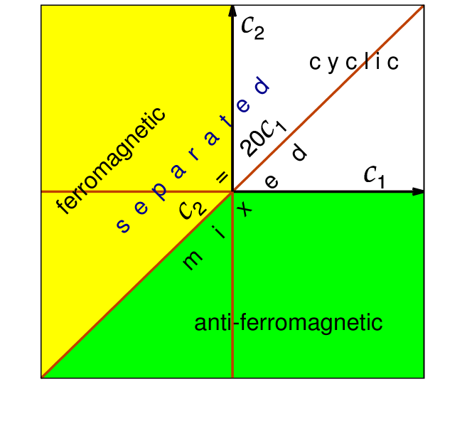
Figure 1: (Color online) The $c_{2}-c_{1}$ phase plot illustrating ferromagnetic, anti-ferromagnetic, and cyclic phases. The $c_{2}=20c_{1}$ line separating the ferromagnetic and anti-ferromagnetic phases as obtained from the present analytic consideration is shown. Separated phase is possible above this line and miscible phase below this line.

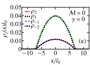
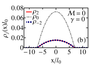
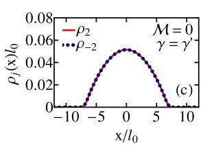
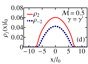
Figure 2: (Color online) Component densities of a ²³Na spinor BEC of $10000$ atoms for $\Omega=0$ and $c_{0}=242.97,c_{1}=12.06>0,$ and $c_{2}=-13.03<20c_{1}$. The parameters used are (a) $\gamma={\cal M}=0$, (b) $\gamma={\cal M}=0$, (c) $\gamma=\gamma^{\prime},{\cal M}=0$, and (d) $\gamma=\gamma^{\prime},{\cal M}=0.5$; here $\gamma^{\prime}$ can have any arbitrary real value including 0, and hence denotes any arbitrary strength of SO coupling. Time-reversal symmetry is broken in (d). In this and following similar figures all quantities are dimensionless and only the nonzero density components are shown.

III.2 Numerical Results

We consider $10000$ atoms of ²³Na (in $f=2$ hyper-fine spin state) in a trapping potential with $\omega_{x}/(2\pi)=20$ Hz and $\omega_{y}/(2\pi)=\omega_{z}/(2\pi)=400$ Hz. The oscillator lengths with this set of parameters are $l_{0}=4.69~{}\mu$m and $l_{yz}=1.05~{}\mu$m. In numerical calculation it is found that all over the ferromagnetic domain of Fig. 1 the density profiles are qualitatively the same always leading to a phase separation. In the anti-ferromagnetic domain the density profiles also remain similar without a phase separation. In the cyclic domain the density profiles are different for $c_{2}>20c_{1}$ and $c_{2}<20c_{1}$, the former leading to a phase separation and the latter leading to a miscible configuration. We will consider these distinct domains in the presentation of results. In addition, in different domains we have different types of symmetry-breaking states, which we will also illustrate.

The background $s$-wave scattering lengths of ²³Na in total spin $f_{\mathrm{tot}}=0,2,$ and $4$ channels are $a_{0}=34.9a_{B}$, $a_{2}=45.8a_{B}$, and $a_{4}=64.5a_{B}$ ueda ; Ciobanu , respectively, where $a_{B}$ is the Bohr radius. With these values of scattering lengths, we have $c_{0}=242.97,c_{1}=12.06>0,$ and $c_{2}=-13.03<20c_{1}$, corresponding to the anti-ferromagnetic domain in Fig. 1. In the absence of SO and Rabi couplings, and magnetization, $\gamma=\Omega={\cal M}=0$, there are more than one degenerate ground states ueda . In Fig. 2 (a) - (c), three such degenerate ground states are illustrated. These states are obtained with different initial choices for the wave-function components in imaginary-time propagation. For these states, some of the wave-function components have zero values. One can also have a state where the two components $j=\pm 1$ are populated with identical density (not illustrated here) as in Fig. 2 (c), which can be generated by a suitable rotation of the state of Fig. 2 (c) in spin space ueda . In the presence of a non-zero SO coupling ($\gamma\neq 0,\Omega={\cal M}=0$), the degeneracy between the various ground states is removed and only the non-degenerate state of Fig. 2 (c) with the components $j=\pm 2$ survives. In this case there is no phase separation as concluded analytically in Sec. II.2. The degeneracy is also removed for non-zero magnetization ($\gamma=\Omega=0,{\cal M}\neq 0$). In this case too, there is only one ground state involving components $j=\pm 2$, whose density profile does not change with the introduction of SO coupling as is shown in Fig. 2 (d). Hence, the degenerate ground states exist only for zero magnetization in the absence of SO coupling.

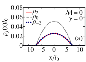
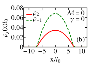
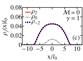
Figure 3: (Color online) Same as in Fig. 2 for $c_{0}=242.97,c_{1}=12.06>0$, and $c_{2}=65.76<20c_{1}.$. The parameters used are (a) $\gamma={\cal M}=0$, (b) $\gamma=0,{\cal M}=0$, (c) $\gamma=1,{\cal M}=0$, and (d) $\gamma=1,{\cal M}=0.5$. Time-reversal symmetry is broken in all cases.

To obtain $c_{1}>0$ and $0<c_{2}<20c_{1}$, we consider $a_{0}=52.35a_{B}$, $a_{2}=45.8a_{B}$, and $a_{4}=64.5a_{B}$, leading to $c_{0}=242.97,c_{1}=12.06>0$, and $c_{2}=65.76<20c_{1}.$ This corresponds to the cyclic domain with miscible states. For ${\cal M}=0$, the ground state solution in the absence of the SO coupling ($\gamma=0$) is shown in Fig. 3 (a), which can be written as $(\phi_{2},\phi_{1},\phi_{0},\phi_{-1},\phi_{-2})^{T}=\sqrt{\rho}(1,0,i\sqrt{2},0,1)^{T}/2$, where $T$ stands for transpose and $\rho$ is the total density. This state has a purely imaginary $\phi_{0}$, a real $\phi_{\pm 2}$ and $\phi_{\pm 1}=0$, and is degenerate with the state $(\phi_{2},\phi_{1},\phi_{0},\phi_{-1},\phi_{-2})^{T}=\sqrt{\rho}(1,0,0,\sqrt{2},0)^{T}/\sqrt{3}$ shown in Fig. 3 (b), where the $\pm j$ symmetry of the states is broken. The latter state has only $j=2,-1$ components. The aforementioned two states break the time-reversal symmetry and are degenerate with their time-reversed counterparts. For a nonzero $\gamma$, the degeneracy between these two states is no longer ensured. With the introduction of a progressively increasing SO coupling $\gamma$, in the state of Fig. 3 (a) $\rho_{0}$ decreases with the corresponding increase in $\rho_{\pm 2}$ as is shown in Fig. 3 (c). With further increase in $\gamma$, $\rho_{0}$ becomes zero and only the components $j=\pm 2$ survive. The introduction of a nonzero magnetization ${\cal M}$ only introduces a splitting in the $j=\pm 2$ components as shown in Fig. 3 (d). There is no phase separation in this case also. Above a critical value of SO coupling $\gamma$, the condensate consists of atoms in only $m_{f}=\pm 2$ states, which for ${\cal M}=0$ is time-reversal symmetric.

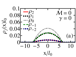
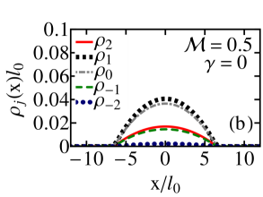
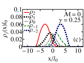
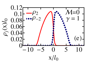
Figure 4: (Color online) Same as in Fig. 2 for $c_{0}=201.36,c_{1}=-1.81,c_{2}=24.15>20c_{1}$. The parameters used are (a) $\gamma={\cal M}=0$, (b) $\gamma=0,{\cal M}=0.5$, (c) $\gamma=0.25,{\cal M}=0$, (d) $\gamma=0.25,{\cal M}=0.5$, (e) $\gamma=1,{\cal M}=0$, and (f) $\gamma=1,{\cal M}=0.5$. Time-reversal symmetry is broken in (b) - (f).

The above study shows that there cannot be a phase separation for $c_{2}<20c_{1}.$ Next we consider $c_{2}>20c_{1}.$ First we consider a ferromagnetic state with $c_{1}<0$ and $c_{2}>0$ obtained by employing $a_{0}=52.35a_{B}$, $a_{2}=45.8a_{B}$, $a_{4}=43.0a_{B}$, leading to $c_{0}=201.36,c_{1}=-1.81,c_{2}=24.15>20c_{1}$. In this case the densities of the spinor BEC of 10000 atoms are shown for $\Omega=0$ for different values of $\gamma$ and ${\cal M}$. in Fig. 4 (a) - (f). From these plots we see that with an increase of SO coupling from $\gamma=0$, the overlapping component states separate and the population of the $j=\pm 2$ components increase at the cost of a reduction in population of the $j=0,\pm 1$ components. Finally, for $\gamma\approx>1$ only the components $j=\pm 2$ survive. In all cases a finite non-zero magnetization ${\cal M}$ breaks the symmetry between densities of the components $j=\pm 1$ and between $j=\pm 2$. The ground state solutions in this case are phase separated for $\gamma$ greater than a critical value in agreement with the discussion in Sec. II.2.

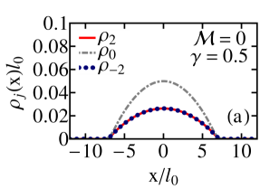
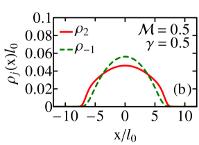
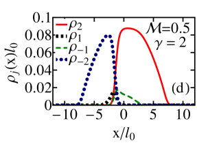
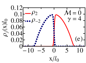
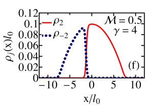
Figure 5: (Color online) Same as in Fig. 2 for $c_{0}=242.97>0,c_{1}=12.06>0$ and $c_{2}=459.68>20c_{1}$. The parameters used are (a) $\gamma=0.5,{\cal M}=0$, (b) $\gamma=0.5,{\cal M}=0.5$, (c) $\gamma=2,{\cal M}=0$, (d) $\gamma=2,{\cal M}=0.5$, (e) $\gamma=4,{\cal M}=0$, and (f) $\gamma=4,{\cal M}=0.5$. Time-reversal symmetry is broken in all cases.

Next we consider a cyclic phase with $c_{2}>20c_{1}$. For this we consider $a_{0}=139.6a_{0}$, $a_{2}=45.8a_{0}$, and $a_{4}=64.5a_{0}$ leading to $c_{0}=242.97>0,c_{1}=12.06>0$ and $c_{2}=459.68>20c_{1}$, corresponding to a cyclic phase. As the strength of SO coupling $\gamma$ is increased, there is a phase separation as is shown in Figs. 5 (c) - (f). The nature of the phase separation in this case is different from that discussed in $c_{1}<0$ and $c_{2}>20c_{1}$ in the sense that the components $j=2$ and $-1$ as well as $-2$ and $1$ are overlapping in this case, consistent with the conclusion of the theoretical analysis in Sec. II.2. The solutions in this domain always break time-reversal symmetry irrespective of the value of $\gamma$.

Symmetry-preserving versus symmetry-breaking solutions: The imaginary-time propagation, that we use in calculation, preserves the symmetry of the initial input wave function. Different types of states can be obtained with different inputs. For example, the states illustrated so far in Figs. 2 $-$ 5 were obtained with Gaussian inputs, which were slightly shifted from the origin, for the component wave functions. We can obtain different density distribution for the components by using initial Gaussian inputs centered at the origin. This is illustrated in Fig. 6 for the same set of parameters as in Fig. 4: $c_{0}=201.36,c_{1}=-1.81,c_{2}=24.15>20c_{1}$. Distinct from Fig. 4, in Fig. 6, the phase separation occurs in a different fashion preserving the symmetry of the trap: $\rho_{j}(x)=\rho_{j}(-x)$. One of the components leaves the central region and stays symmetrically on both sides of the origin. The symmetry-breaking states of Fig. 4 have lower energy than the symmetry-preserving states of Fig. 6 with the same sets of parameters. Similar symmetry-breaking states were found in scalar binary condensates Esry . In symmetry-preserving and symmetry-breaking cases the phase separation may start with different values of magnetization ${\cal M}$ and SO coupling $\gamma$. The magnetization and SO couplings in Figs. 6 (b) and (c) are identical to those in Figs. 4 (e) and (d), respectively. For the same set of parameters, there is a phase separation in Fig. 4 (d) and not in Fig. 6 (c). In Fig. 6 the phase separation starts at a larger value of SO coupling.

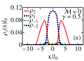
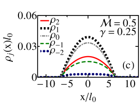
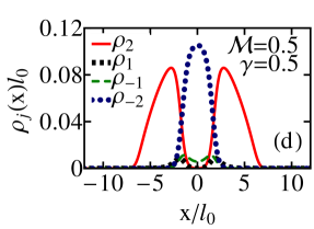
Figure 6: (Color online) Same as in Fig. 2 for $c_{0}=201.36,c_{1}=-1.81,c_{2}=24.15>20c_{1}$. The parameters used are (a) $\gamma=0.5,{\cal M}=0$, (b) $\gamma=1,{\cal M}=0$, (c) $\gamma=0.25,{\cal M}=0.5$, and (d) $\gamma=0.5,{\cal M}=0.5$. Time-reversal symmetry is broken in all cases.

Next we show in Fig. 7 some of the possible parity-breaking states obtained with the parameters of Fig. 2 (c), e.g., $c_{0}=242.97,c_{1}=12.06>0,c_{2}=-13.03<20c_{1}$. Figures 7 (a) and (b) were calculated with real Gaussian inputs for both the $j=\pm 2$ components. This will correspond to $\alpha_{2}=\alpha_{-2}=1/\sqrt{2}$ in the discussion in Sec. II.2, leading to symmetry properties ${\cal R}[\phi_{\pm 2}(x)]={\cal R}[\phi_{\pm 2}(-x)],$ ${\cal I}[\phi_{\pm 2}(x)]=-{\cal I}[\phi_{\pm 2}(-x)],$ ${\cal R}[\phi_{2}(x)]={\cal R}[\phi_{-2}(x)],$ ${\cal I}[\phi_{2}(x)]=-{\cal I}[\phi_{-2}(x)]$, as illustrated in Fig. 7 (a) and (b). Figures 7 (c) and (d) were calculated with an imaginary Gaussian input for $j=2$ and a real Gaussian input for $j=-2$ components. This will correspond to $\alpha_{2}=i/\sqrt{2}$ and $\alpha_{-2}=1/\sqrt{2}$ in the discussion in Sec. II.2, leading to symmetry properties ${\cal R}[\phi_{2}(x)]=-{\cal R}[\phi_{2}(-x)],$ ${\cal R}[\phi_{-2}(x)]={\cal R}[\phi_{-2}(-x)],$ ${\cal I}[\phi_{2}(x)]={\cal I}[\phi_{2}(-x)],$ ${\cal I}[\phi_{-2}(x)]=-{\cal I}[\phi_{-2}(-x)],$ ${\cal R}[\phi_{2}(x)]={\cal I}[\phi_{-2}(x)],$ ${\cal I}[\phi_{2}(x)]={\cal R}[\phi_{-2}(x)],$ as illustrated in Fig. 7 (c) and (d). In the same fashion all the parity-breaking states obtained in Sec. II.2 from an analytic consideration can be realized numerically.

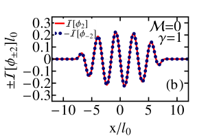
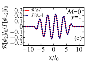
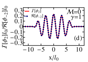
Figure 7: Real and imaginary parts of the $j=\pm 2$ wave-function components for the parameters of Fig. 2 (c). Plots (a) and (b) were obtained with two real Gaussian input states for $j=\pm 2$ components. Plots (c) and (d) were obtained with an imaginary Gaussian input for $j=2$ and a real Gaussian input for $j=-2$ components.

As in the case of a binary condensate Ao , phase-separated SO-coupled spinor condensates can be categorized either as weakly segregated or strongly segregated. In the weakly segregated domain, the total density profile preserves the symmetry of the trapping potential (not illustrated here) and has an approximate smooth Gaussian profile like that of a single-component BEC in a trap. In the strongly segregated domain, a notch appears in the total density profile corresponding to symmetry breaking solutions shown in Figs. 4 (e), (f), 5 (e) and 5 (f). In case of a non-zero magnetization, asymmetrically located notch ensures that the total density profiles corresponding to Figs. 4 (f) and 5 (f) do not not have the symmetry of the trap (not shown here).

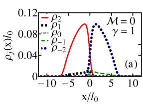
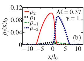
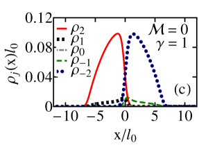
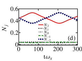
Figure 8: Dynamics of a phase-separated spinor condensate in the presence of both SO coupling and Rabi term ($\gamma=1.0,\Omega=0.5$ and a zero initial magnetization. (a) The density profiles at $t=0$, (b) the densities at $\omega_{x}t=70.0$, and (c) the densities at $\omega_{x}t=275$, the time after which the condensate has recovered its initial shape after one complete oscillation. (d) The component population $N_{j}=\int\rho_{j}(x)dx$ versus time during a complete cycle of the periodic oscillation.

Spin-mixing dynamics in a phase-separated spinor condensate: In the presence of a Rabi term ($\Omega\neq 0$) the solutions of Eqs. (20) - (24), in general, are not stationary and exhibit oscillating spin-mixing dynamics H_Wang ; Pu . To study the spin-mixing dynamics in a phase-separated spinor condensate, we again consider $10000$ atoms of ²³Na with $a_{0}=52.35a_{B}$, $a_{2}=45.8a_{B}$ $a_{4}=43.0a_{B}$, as in Fig. 4, yielding $c_{0}=201.36,c_{1}=-1.81,c_{2}=24.15>20c_{1}$. We first solve Eqs. (20) - (24) using imaginary-time propagation employing $\gamma=1,{\cal M}=0$ and $\Omega=0.5$ with the aforementioned set of parameters. The initial component densities so obtained are shown in Fig. 8 (a). We then evolve this solution using real-time propagation. The presence of the Rabi term leads to spin-mixing between the various components. The magnetization ${\cal M}$ is no longer a conserved parameter in the presence of the Rabi term as can be interpreted from Fig. 8 (b), where the magnetization is $0.37$ at time $\omega_{x}t=70$. During the evolution, the condensate densities execute oscillation periodically recovering the initial shape as shown in Fig. 8 (c) at time $\omega_{x}t=275$ after one complete oscillation. In Fig. 8 (d) we plot the component normalizations $N_{j}$ versus time during this periodic oscillation.

IV Summary of results

We studied the density profile of a trapped SO-coupled $f=2$ BEC for different values of the inter-atomic scattering lengths. Such modification of the scattering lengths can be realized in a laboratory using the Feshbach resonance technique fesh . The Hamiltonian of this problem preserves time-reversal symmetry but breaks parity. The wave functions of the different spin components are complex in general. In the anti-ferromagnetic domain only miscible density profile of different components are found. In this domain the wave functions preserve time-reversal symmetry. In the ferromagnetic domain phase-separated density profile of different components are found. The underlying wave functions could be degenerate and break time reversal symmetry in this domain with time-reversal operator connecting two degenerate wave functions. A class of parity-breaking states are found where the real and imaginary parts of wave functions exhibit opposite parities. These conclusions were illustrated by a numerical solution of a mean-field model

References

• (1) D. M. Stamper-Kurn, M. R. Andrews, A. P. Chikkatur, S. Inouye, H.-J. Miesner, J. Stenger, and W. Ketterle, Phys. Rev. Lett. 80, 2027 (1998); J. Stenger, S. Inouye, D. M. Stamper-Kurn, H.-J. Miesner, A. P. Chikkatur, and W. Ketterle, Nature 396, 345 (1998).
• (2) Y. Kawaguchi and M. Ueda, Phys. Rep. 520, 253 (2012).
• (3) D. M. Stamper-Kurn and M. Ueda, Rev. Mod. Phys. 85, 1191 (2013).
• (4) T. Ohmi, and K. Machida, J. Phys. Soc. Japan, 67, 1822 (1998).
• (5) T. L. Ho, Phys. Rev. Lett. 81, 742 (1998).
• (6) M. Koashi and M. Ueda, Phys. Rev. Lett. 84, 1066 (2000).
• (7) C. V. Ciobanu, S.-K. Yip, and T.-L. Ho, Phys. Rev. A 61, 033607 (2000).
• (8) S. Gautam and S. K. Adhikari, Phys. Rev. A90, 043619 (2014).
• (9) L. Salasnich, A. Parola, and L. Reatto, Phys. Rev. A 65, 043614 (2002).
• (10) K. Osterloh, M. Baig, L. Santos, P. Zoller, and M. Lewenstein, Phys. Rev. Lett. 95, 010403 (2005); J. Ruseckas, G. Juzeliūnas, P. Öhberg, and M. Fleischhauer, Phys. Rev. Lett. 95, 010404 (2005).
• (11) J. Higbie and D. M. Stamper-Kurn, Phys. Rev. Lett. 88, 090401 (2002); T. L. Ho and S. Zhang, Phys. Rev. Lett. 107, 150403 (2011); Y. Deng, J. Cheng, H. Jing, C. P. Sun, and S. Yi, Phys. Rev. Lett. 108, 125301 (2012); J. Radic, T. A. Sedrakyan, I. B. Spielman, and V. Galitski, Phys. Rev. A 84, 063604 (2011).
• (12) Y. A. Bychkov and E. I. Rashba, J. Phys. C 17, 6039 (1984).
• (13) G. Dresselhaus, Phys. Rev. 100, 580 (1955).
• (14) X.-J. Liu, M. F. Borunda, X. Liu, and J. Sinova, Phys. Rev. Lett. 102, 046402 (2009).
• (15) Y.-J. Lin, K. Jiménez-García, and I. B. Spielman, Nature 471, 83 (2011).
• (16) V. Galitski and I. B. Spielman, Nature 494, 49 (2013).
• (17) J.-Y. Zhang, S.-C. Ji, Z. Chen, L. Zhang, Z.-D. Du, B. Yan, G.-S. Pan, B. Zhao, Y.-J. Deng, H. Zhai, S. Chen, and J.-W. Pan, Phys. Rev. Lett. 109, 115301 (2012); C. Qu, C. Hamner, M. Gong, C. Zhang, and P. Engels, Phys. Rev. A 88, 021604(R) (2013); M. Aidelsburger, M. Atala, and S. Nascimb´ene et al., Phys. Rev. Lett. 107, 255301 (2011); Z. Fu, P. Wang, and S. Chai, L. Huang, and J. Zhang, Phys. Rev. A 84, 043609 (2011).
• (18) G. Juzeliūnas, J. Ruseckas, and J. Dalibard, Phys. Rev. A 81, 053403 (2010); J. Dalibard et al., Rev. Mod. Phys. 83, 1523 (2011).
• (19) Z. Lan and P. Öhberg, Phys. Rev. A89, 023630 (2014).
• (20) P. Wang, Z.-Q. Yu, Z. Fu, J. Miao, L. Huang, S. Chai, H. Zhai, and J. Zhang, Phys. Rev. Lett. 109, 095301 (2012); L. W. Cheuk, A. T. Sommer, Z. Hadzibabic, T. Yefsah, W. S. Bakr, and M. W. Zwierlein, Phys. Rev. Lett. 109, 095302 (2012).
• (21) C. Wang, C. Gao, C-M Jian, and H. Zhai, Phys. Rev. Lett. 105, 160403 (2010); A. Aftalion and P. Mason, Phys. Rev. A 88, 023610 (2013); R. Gupta, G. S. Singh, and J. Bosse, Phys. Rev. A 88, 053607 (2013); Q.-Q. Lu and D. E. Sheehy, Phys. Rev. A 88, 043645 (2013).
• (22) T. D. Stanescu, B. Anderson, and V. Galitski, Phys. Rev. A 78, 023616 (2008); S.-K. Yip, Phys. Rev. A 83, 043616 (2011); C.-J Wu, I. Mondragon-Shem, and X.-F. Zhou, Chin. Phys. Lett. 28, 097102 (2011); Q. Zhou and X. Cui, Phys. Rev. Lett. 110, 140407 (2013); S. Gopalakrishnan, A. Lamacraft, and P. M. Goldbart, Phys. Rev. A 84, 061604(R) (2011); H. Hu, B. Ramachandhran, H. Pu, and X.-J. Liu, Phys. Rev. Lett. 108, 010402 (2012); B. Ramachandhran, B. Opanchuk, X.-J. Liu, H. Pu, P. D. Drummond, and H. Hu, Phys. Rev. A 85, 023606 (2012); S. Sinha, R. Nath, and L. Santos, Phys. Rev. Lett. 107, 270401 (2011); T. Ozawa and G. Baym, Phys. Rev. A 85, 013612 (2012); Y. Zhang, L. Mao, and C. Zhang, Phys. Rev. Lett. 108, 035302 (2012); K. Riedl, C. Drukier, P. Zalom, and P. Kopietz, Phys. Rev. A 87, 063626 (2013); Y. Deng, J. Cheng, H. Jing, and S. Yi, Phys. Rev. Lett. 112, 143007 (2014).
• (23) E. Ruokokoski, J. A. M. Huhtamäki, and M. Möttönen, Phys. Rev A 86, 051607(R) (2012); S.-W. Su, I.-K. Liu, Y.-C. Tsai, W. M. Liu, and S.-C. Gou, Phys. Rev. A 86, 023601 (2012); S.-W. Song, Y.-C. Zhang, L. Wen, and H. Wang, J. Phys. B 46, 145304 (2013); S.-W. Song, Y.-C. Zhang, H. Zhao, X. Wang, and W.-M. Liu, Phys. Rev. A 89, 063613 (2014).
• (24) T. Kawakami, T. Mizushima, and K. Machida, Phys. Rev. A 84, 011607(R) (2011); Z. F. Xu, R. Lü, and L. You, Phys. Rev. A 83, 053602 (2011); Z. F. Xu, Y. Kawaguchi, L. You, and M. Ueda, Phys. Rev. A 86, 033628 (2012).
• (25) F. Zhou, Phys. Rev. Lett. 87, 080401 (2001); W. Zhang, S. Yi, and L. You, New J. Phys. 5, 77 (2003); K. Murata, H. Saito, and M. Ueda, Phys. Rev. A 75, 013607 (2007);
• (26) M. Matuszewski, T. J. Alexander, and Y. S. Kivshar, Phys. Rev. A 80, 023602 (2009); M. Matuszewski, Phys. Rev. A 82, 053630 (2010).
• (27) G.-P. Zheng, Y.-G. Tong, and F.-L. Wang, Phys. Rev. A 81, 063633 (2010); H. Saito and M. Ueda, Phys. Rev. A 72, 053628 (2005).
• (28) M. A. Garcia-March, G. Mazzarella, L. Dell’Anna, B. Juliá-Díaz, L. Salasnich, and A. Polls, Phys. Rev. A 89, 063607 (2014).
• (29) J. Larson, J.-P. Martikainen, A. Collin, and E. Sjöqvist, Phys. Rev. A 82, 043620 (2010).
• (30) H. Sakaguchi, Ben Li, and B. A. Malomed, Phys. Rev. E 89, 032920 (2014); Y. Xu, Y. Zhang, and B. Wu, Phys. Rev. A 87, 013614 (2013); O. Fialko, J. Brand, and U. Z¨ulicke, Phys. Rev. A 85, 051605(R) (2012); Y.-K. Liu and S.-J. Yang, Euro. Phys. Lett. 108, 30004 (2014).
• (31) P.-S. He, Y.-H. Zhu, and W.-M. Liu Phys. Rev. A 89, 053615 (2014).
• (32) M. Merkl, A. Jacob, F. E. Zimmer, P. Öhberg, and L. Santos, Phys. Rev. Lett. 104, 073603 (2010).
• (33) T. Ozawa, L. P. Pitaevskii, and S. Stringari, Phys. Rev. A 87, 063610 (2013); D. W. Zhang, J. P. Chen, C. J. Shan, Z. D. Wang, and S. L. Zhu, Phys. Rev. A 88, 013612 (2013); Q. Zhu, C. Zhang and B. Wu, Europhys. Lett. 100, 50003 (2012); D. Toniolo and J. Linder, Phys. Rev. A 89, 061605(R) (2014).
• (34) H. Wang, J. Comput. Phys., 230, 6155 (2011); 274, 473 (2014).
• (35) Y. Li, G. I. Martone, L. P. Pitaevskii, and S. Stringari, Phys. Rev. Lett. 110, 235302 (2013); Y. Zhang and C. Zhang, Phys. Rev. A 87, 023611 (2013); L. Salasnich and B. A. Malomed, Phys. Rev. A 87, 063625 (2013); D. A. Zezyulin, R. Driben, V. V Konotop, and B. A. Malomed, Phys. Rev. A 88, 013607 (2013); Y. Cheng, G. Tang, and S. K. Adhikari, Phys. Rev. A 89, 063602 (2014).
• (36) P. Ao and S. T. Chui, Phys. Rev. A 58, 4836 (1998); P. Facchi, G. Florio, S. Pascazio, and F. V. Pepe, J. Phys. A: Math. Theor. 44 505305 (2011).
• (37) S. Gautam and D. Angom, J. Phys. B 44, 025302 (2011); S. Gautam and D. Angom, J. Phys. B 43, 095302 (2010).
• (38) P. Muruganandam and S. K. Adhikari, Comput. Phys. Commun. 180, 1888 (2009); D. Vudragovic, I. Vidanovic, A. Balaz, P. Muruganandam, and S. K. Adhikari. Comput. Phys. Commun. 183, 2021 (2012).
• (39) W. Bao and F. Y. Lim, Siam J. Sci. Comp. 30, 1925 (2008); F. Y. Lim and W. Bao, Phys. Rev. E 78, 066704 (2008).
• (40) W. Bao and Q. Du, Siam J. Sci. Comp. 25, 1674 (2004).
• (41) W. H. Press. S. A Teukolsky, W. T. Vetterling, and B. P. Flannrey, Numerical Recipies in Fortran 77 , Cambridge University Press, 2nd Edition, (1992).
• (42) B. D. Esry and C. H. Greene, Phys. Rev. A 59, 1457 (1999); S. T. Chui and P. Ao, Phys. Rev. A 59, 1473 (1999).
• (43) H. Pu, C. K. Law, S. Raghavan, J. H. Eberly, and N. P. Bigelow, Phys. Rev. A 60, 1463 (1999).
• (44) S. Inouye et al., Nature (London) 392, 151 (1998).