The Needle in the 100 deg² Haystack: Uncovering Afterglows of Fermi GRBs With the Palomar Transient Factory

Abstract

The Fermi Gamma–ray Space Telescope has greatly expanded the number and energy window of observations of gamma-ray bursts. However, the coarse localizations of tens to a hundred square degrees provided by the Fermi GRB Monitor instrument have posed a formidable obstacle to locating the bursts’ host galaxies, measuring their redshifts, and tracking their panchromatic afterglows. We have built a target–of–opportunity mode for the intermediate in order to perform targeted searches for Fermi afterglows. Here, we present the results of one year of this program: 8 afterglow discoveries out of 35 searches. Two of the bursts with detected afterglows (GRBs 130702A and 140606B) were at low redshift ($z=0.145$ and 0.384 respectively) and had spectroscopically confirmed broad–line Type Ic supernovae. We present our broadband follow–up including spectroscopy as well as X–ray, UV, optical, millimeter, and radio observations. We study possible selection effects in the context of the total Fermi and Swift GRB samples. We identify one new outlier on the Amati relation. We find that two bursts are consistent with a mildly relativistic shock breaking out from the progenitor star, rather than the ultra–relativistic internal shock mechanism that powers standard cosmological bursts. Finally, in the context of the Zwicky Transient Facility, we discuss how we will continue to expand this effort to find optical counterparts of binary neutron star mergers that may soon be detected by Advanced LIGO and Virgo.

2015 June 8

1. Introduction

Deep synoptic optical surveys, including the Palomar Transient Factory (PTF; Law et al. 2009; Rau et al. 2009) and Pan–STARRS (Kaiser et al., 2010), have revealed a wealth of new transient and variable phenomena across a wide range of characteristic luminosities and timescales (Kasliwal, 2011). With a wide (7 deg²) instantaneous field of view (FOV), moderately deep sensitivity (reaching $R=20.6$ mag in 60 s), a consortium of follow-up telescopes, sophisticated image subtraction and machine learning pipelines, and an international team of human–in–the–loop observers, Palomar Transient Factory (PTF) has been a wellspring of new or rare kinds of explosive transients (for instance, Quimby et al. 2011; Kasliwal et al. 2012) and early–time observations of supernova or their progenitors (see, for example, Nugent et al. 2011; Corsi et al. 2012; Ofek et al. 2013; Gal-Yam et al. 2014). PTF has even blindly detected the optical emission (Cenko et al. 2014; S. B. Cenko et al., in preparation) from the rarest, brightest, and briefest of all known cosmic explosions, GRBs, hitherto only discoverable with the aid of precise localizations from space–based gamma–ray observatories. PTF has also detected explosions that optically resemble GRB afterglows but may entirely lack gamma–ray emission (Cenko et al., 2013b).

GRBs and their broadband afterglows are notoriously challenging to capture. They naturally evolve from bright to faint, and from high (gamma- and hard X–ray) to low (optical and radio) photon energies, with information encoded on energy scales from 1 to $10^{16}$ GHz (Perley et al., 2014d) and timescales from $10^{-3}$ to 10⁷ s. Only with a rapid sequence of handoffs between facilities graded by energy passband, FOV, and position accuracy have we been able to find them, pinpoint their host galaxies, and constrain their physics. The Swift mission (Gehrels et al., 2004), with its 1.4 sr–wide (50% coded) Burst Alert Telescope (BAT; Barthelmy et al. 2005) and its ability to slew and train its onboard X–ray Telescope (XRT; Burrows et al. 2005) and UV/Optical Telescope (UVOT; Roming et al. 2005) on the location of a new burst within 100 s, has triumphed here: in nine years of operation, it has tracked down $\approx 700$ X–ray afterglows and enabled extensive panchromatic observations by a worldwide collaboration of ground–based optical and radio facilities.

Meanwhile, the Fermi satellite has opened up a new energy regime extending up to 300 GeV, with the Large Area Telescope (LAT; Atwood et al. 2009) detecting high–energy photons for about a dozen bursts per year. The Gamma-ray Burst Monitor (GBM; Meegan et al. 2009), an all–sky instrument sensitive from 8 keV to 40 MeV, detects GRBs prolifically at a rate of $\approx 250$ yr^-1, with a large number (about 44 yr^-1) belonging to the rarer short, hard bursts (Paciesas et al., 2012a). Although Large Area Telescope (LAT) can provide localizations that are as accurate as $\sim$10′, Fermi Gamma-ray Burst Monitor (GBM) produces error circles that are several degrees across. Since most bursts seem to lack GeV emission detectable by LAT, most Fermi GBM bursts do not receive deep, broadband follow–up. Consequently, their redshifts and the properties of their afterglows have remained largely unknown.

As part of the intermediate (iPTF), over the past year we have developed the ability to rapidly tile these $\sim 100$ deg² GBM error circles and pinpoint the afterglows. This target–of–opportunity (TOO) capability uses and briefly redirects the infrastructure of our ongoing synoptic survey (the operation of which is discussed in Gal-Yam et al. 2011), notably the machine learning software and the instrumental pipeline composed of the Palomar 48 inch Oschin telescope (P48; Rahmer et al. 2008), the robotic Palomar 60 inch telescope (P60; Cenko et al. 2006), and associated spectroscopic resources including the Palomar 200 inch Hale telescope (P200).

In Singer et al. (2013b), we announced the first discovery of an optical afterglow based solely on a Fermi GBM localization. That explosion, GRB 130702A/iPTF13bxl, was noteworthy for several reasons. First, it was detected by Fermi LAT. Second, it was at moderately low redshift, $z=0.145$, yet had prompt energetics that bridged the gap between “standard,” bright cosmically distant bursts and nearby sub–luminous bursts and X–ray flashes. Third, due to its low redshift, an accompanying SN was spectroscopically detectable.

In this work, we begin with a detailed description of the operation of the iPTF GRB afterglow search. We then present seven more GBM–iPTF afterglows from the first 13 months of this project. In each of the eight cases, the association between the optical transient and the GRB was proven by the presence of high–redshift absorption lines in the optical spectra and the coincident detection of a rapidly fading X–ray source with Swift X–ray Telescope (XRT). In two cases, the positions were further corroborated by accurate Fermi LAT error circles, and in four cases by accurate InterPlanetary Network (IPN) triangulations involving distant spacecraft. In one case (GRB 140508A), the IPN triangulation was performed rapidly and was instrumental in selecting which optical transient candidates to follow up. In six cases, radio afterglows were detected. Our discovery rate of 8 out of 35 events is consistent with the ages and searched areas of the GBM bursts, combined with the luminosity function of optical afterglows. Consequently, by tiling larger areas and/or stacking exposures, the iPTF afterglow search should be able to scale to coarser localizations and fainter optical signals, such as those associated with short GRBs.

Next, we present extensive follow–up observations, including $R$–band photometry from the Palomar 48 inch Oschin telescope (P48), multicolor photometry from the robotic Palomar 60 inch telescope (P60), spectroscopy (acquired with the P200, Keck, Gemini, APO, Magellan, Very Large Telescope (VLT), and GTC), and radio observations with the Karl G. Jansky Very Large Array (VLA), the Combined Array for Research in Millimeter–wave Astronomy (CARMA; Bock et al. 2006; Corder et al. 2010), the Australia Telescope Compact Array (ATCA; Frater et al. 1992), and the Arcminute Microkelvin Imager (AMI; Zwart et al. 2008). We provide basic physical interpretations of the broadband spectral energy distributions of these afterglows. We find that seven of the events are consistent with the classic model of synchrotron cooling of electrons that have been accelerated by a single forward shock encountering either the constant-density circumburst interstellar medium (ISM; broadband behavior predicted in Sari et al. 1998) or a stellar (i.e., Wolf—Rayet) wind environment (Chevalier & Li, 1999). The possible exception, GRB 140620A/iPTF14cva, can probably be explained by standard extensions of this model, a reverse shock or an inverse Compton component.

Two of the afterglows (GRB 130702A/iPTF13bxl and GRB 140606B/iPTF14bfu) faded away to reveal spectroscopically detected broad–line Type Ic . Despite the abundant photometric evidence for SNe in afterglow light curves (see Li & Hjorth 2014 and references therein), the distinction of SN spectroscopy has been shared by scarcely tens out of $\approx$800 long Swift bursts in nine years of operation.

We estimate the kinetic energies of the relativistic blast waves of these events from their X–ray afterglows (Freedman & Waxman, 2001). We find that although the gamma–ray energetics of these eight bursts are broadly similar to the Swift sample, two low–luminosity bursts (GRBs 130702A and 140606B) have significantly lower kinetic energies. We discuss the possibility that these two bursts arise not from a standard ultra–relativistic internal shock, but from a mildly relativistic shock as it breaks out from the progenitor star (see, for example, Nakar & Sari 2012).

We conclude by discussing prospects for targeted optical transient searches in wide areas. This is especially relevant for optical counterparts of gravitational wave (GW) events. We illustrate that optical afterglows of short bursts, which are intimately linked to the prime sources for the Advanced Laser Interferometer Observatory (LIGO) and Virgo, should be well within the reach of a similar approach using Zwicky Transient Facility (ZTF; Kulkarni 2012; Bellm 2014; Smith et al. 2014).

2. Search Methodology

We begin by describing our TOO observations and afterglow search step by step.

2.1. Automated TOO Marshal: Alerts and Tiling

A program called the iPTF TOO Marshal monitors the stream of Gamma-ray Coordinates Network (GCN) notices from the three redundant, anonymous NASA/GSFC VOEvent servers. It listens for notices of type FERMI_GBM_GND_POS, sent by GBM’s automated on–ground localization, or FERMI_GBM_FIN_POS, sent by the GBM burst advocate’s human–in–the–loop localization.

Upon receiving either kind of notice, the TOO Marshal determines if the best-estimate sky position is observable from Palomar at any time within the 24 hr after the trigger. The criterion for observability is that the position is at an altitude $>23\fdg 5$ (i.e. airmass $\lesssim 2.5$), at least $20\arcdeg$ from the center of the moon, at an hour angle between $\pm 6\fh 5$, and that the Sun is at least $12\arcdeg$ below the horizon at Palomar.

If the position is observable and the 1$\sigma$ statistical error radius $r_{\mathrm{stat}}$ reported in the GCN notice is less than $10\arcdeg$, the TOO Marshal selects a set of 10 P48 fields that optimally cover the error region. It converts the GBM position estimate and radius into a probability distribution by applying a well–known empirical prescription of the systematic errors of the GBM localization. Paciesas et al. (2012b) state that the total effective error radius in the FERMI_GBM_FIN_POS localizations is well described by the quadrature sum of the statistical radius and a systematic contribution, where the systematic is $2\fdg 6$ for 72% of bursts and $10\fdg 4$ for 28% of bursts. We use the weighted rms of these two values, $r_{\mathrm{sys}}=\sqrt{0.72(2\fdg 6)^{2}+0.28(10\fdg 4)^{2}}\approx 6\arcdeg$. The total error radius is then $r_{\mathrm{eff}}=\sqrt{{r_{\mathrm{stat}}}^{2}+{r_{\mathrm{sys}}}^{2}}$. We construct a Fisher—von Mises distribution, centered on the best–estimate position, with a concentration parameter of

$$\kappa=\left[1-\cos\left(\frac{\pi}{180\arcdeg}r_{\mathrm{eff}}\right)\right]^{-1}.$$ (1)

With the FERMI_GBM_FIN_POS alert, the Fermi GBM team also distributes a detailed localization map that accounts for the systematic effects (Connaughton et al., 2015). The TOO Marshal retrieves from the Fermi data archive a file that describes the 1$\sigma$, 2$\sigma$, and 3$\sigma$ significance contours. If the localization has significant asymmetry, we also retrieve a 2D FITS image whose pixel values correspond to the GBM localization significance, and use this instead of the Fisher—von Mises distribution.

Giving preference to fields for which deep co–added reference images exist, the TOO Marshal selects 10 P48 fields spanning an area of $\approx 72$ deg² to maximize the probability of enclosing the true (but as yet unknown) location of the source, assuming the above distribution.

The Marshal then immediately contacts a team of humans (the authors) by SMS text message, telephone, and e-mail. The humans are directed to a mobile–optimized web application to trigger the P48 (see Fig. 11).

2.2. Triggering the P48

Within the above constraints, we decide whether to follow up the burst based on the following criteria. The event must be $\lesssim$12 hr old when it first becomes observable from Palomar, and we must cover enough of the error circle to have a $\gtrsim$30% chance of enclosing the position of the source. We discard any bursts that are detected and accurately localized by Swift BAT, because these are more efficiently followed up by conventional means. We also give preference to events that are out of the Galactic plane and that are observable for at least 3 hr.

There are some exceptional circumstances that override these considerations. If the burst’s position estimate is accessible within an hour after the burst, we may select it even if the observability window is very brief. If the burst is very well localized or has the possibility of a substantially improved localization later due to a LAT or IPN detection, we may select it even if it is in the Galactic plane.

The default observing program is three epochs of P48 images at a 30–minute cadence. The human may shorten or lengthen the cadence if the burst is very young or old (see the discussion of Equation (2) in Section 2.4 below), change the number of epochs, or add and remove P48 fields. When the human presses the “Go” button, the TOO Marshal sends a machine-readable e-mail to the P48 robot. The robot adds the requested fields to the night’s schedule with the highest possible priority, ensuring that they are observed as soon as they are visible.

2.3. Automated Candidate Selection

As the night progresses, the TOO Marshal monitors the progress of the observations and the iPTF real–time image subtraction pipeline (P. E. Nugent et al. 2015, in preparation). The real–time pipeline creates difference images between the new P48 observations and co–added references composed of observations from months or years earlier. It generates candidates by performing source extraction on the difference images. A machine learning classifier assigns a real/bogus score (RB2; Brink et al. 2013) to each candidate that predicts how likely the candidate is to be a genuine astrophysical source (rather than a radiation hit, a ghost, an imperfect image subtraction residual, or any other kind of artifact).

Table 1 lists the number of candidates that remain after each stage of candidate selection. First, requiring candidates to have signal–to–noise ratio (S/N)$>5$ gives us a median of 35,000 candidates. This number varies widely with galactic latitude and the area searched (a median of $\sim$500 deg^-2). Second, we only select candidates that have RB2$>0.1$, reducing the number of candidates to a median of 36% of the original list. Third, we reject candidates that coincide with known stars in reference catalogs ( Sloan Digital Sky Survey (SDSS) and the PTF reference catalog), cutting the list to 17%. Fourth, we eliminate asteroids cataloged by the Minor Planet Center, reducing the list to 16%. Fifth, we demand at least two secure P48 detections after the GBM trigger, reducing the list to a few percent, or $\sim 500$ candidates.

When the image subtraction pipeline has finished analyzing at least two successive epochs of any one field, the TOO Marshal contacts the humans again and the surviving candidates are presented to the humans via the Treasures portal.

Table 1Number of Optical Transient Candidates Surviving Each Vetting Stage

	S/N	RB2	Not	Not in	Detected	Saved for
GRB	$>5$	$>0.1$	Stellar	MPC	Twice	Follow–up	RB2
130702A	14 629	2 388	1 346	1 323	417	11	0.843
131011A	21 308	8 652	4 344	4 197	434	23	0.198
131231A	9 843	2 503	1 776	1 543	1 265	10	0.137
140508A	48 747	22 673	9 970	9 969	619	42	0.730
140606B	68 628	26 070	11 063	11 063	1 449	28	0.804
140620A	152 224	50 930	17 872	17 872	1 904	34	0.826
140623A	71 219	29 434	26 279	26 279	442	23	0.873
140808A	19 853	4 804	2 349	2 349	79	12	0.318
Median reduction		36%	17%	16%	1.7%	0.068%

2.4. Visual scanning in Treasures Portal

The remaining candidate vetting steps currently involve human participation and are informed by the nature of the other transients that iPTF commonly detects: foreground SNe (slowly varying and in low–$z$ host galaxies), active galactic nuclei, cataclysmic variables, and M–dwarf flares.

In the Treasures portal, we visually scan through the automatically selected candidates one P48 field at a time, examining $\sim$10 objects per field (see Figure 12 for a screenshot of the Treasures portal). We visually assess each candidate’s image subtraction residual compared to the neighboring stars of similar brightness in the new image. If the residual resembles the new image’s point-spread function, then the candidate is considered likely to be a genuine transient or variable source.

Next, we look at the photometric history of the candidates. Given the time, $t$, of the optical observation relative to the burst and the cadence, $\delta t$, we expect that a typical optical afterglow that decays as a power law $F_{\nu}\propto t^{-\alpha}$, with $\alpha=1$, would fade by $\delta m=2.5\log_{10}(1+\delta t/t)$ mag over the course of our observations. Any source that exhibits statistically significant fading ($\delta m/m\gg 1$) consistent with an afterglow decay becomes a prime target.

Note that a $1\sigma$ decay in brightness requires such a source to be

$$-2.5\log_{10}\left(\frac{\delta t}{t\sqrt{2}}\right)$$ (2)

brighter than the $1\sigma$ limiting magnitude of the exposures. For example, given the P48’s typical limiting magnitude of $R=20.6$ and the standard cadence of $\delta t=0.5$ hr, if a burst is observed $t=3$ hr after the trigger, its afterglow may be expected to have detectable photometric evolution only if it is brighter than $R=18.3$. Noting that long GRBs preferentially occur at high redshifts and in intrinsically small, faint galaxies (Svensson et al., 2010), we consider faint sources that do not display evidence of fading if they are not spatially coincident with any sources in SDSS or archival iPTF observations.

If a faint source is near a spatially resolved galaxy, then we compute its distance modulus using the galaxy’s redshift or photometric redshift from SDSS. We know that long GRB optical afterglows at $t=1$ day typically have absolute magnitudes of $-25<M_{B}<-21$ mag (1$\sigma$ range; see Figure 9 of Kann et al. 2011). Most SNe are significantly fainter: Type Ia are typically $M_{B}\sim-19$ mag whereas Ibc and II are $M_{B}\sim-17$ mag, with luminous varieties of both Type Ibc and II extending to $M_{B}\sim-19$ mag (Richardson et al., 2002; Li et al., 2011). Therefore, if the candidate’s presumed host galaxy would give it an absolute magnitude $M_{R}<-20$ mag, it is considered promising. This criterion is only useful for long GRBs because short GRB afterglows are typically $\sim 6$ mag fainter than long GRB afterglows (Kann et al., 2011).

The human saves all candidates that are considered promising by these measures to the iPTF Transient Marshal database. This step baptizes them with an iPTF transient name, which consists of the last two digits of the year and a sequential alphabetic designation.

2.5. Archival vetting in the Transient Marshal

Once named in the Transient Marshal, we perform archival vetting of each candidate using databases including VizieR (Ochsenbein et al., 2000), NED, the High Energy Astrophysics Science Archive Research Center (HEASARC), and Catalina Real-time Transient Survey (Drake et al., 2009), in order to check for any past history of variability at that position (see Figure 13 for a screenshot of the Transient Marshal).

We check for associations with known quasars or AGNs in Véron-Cetty & Véron (2010) or with AGN candidates in Flesch (2010).

M dwarfs can produce bright, blue, rapidly fading optical flares than can mimic optical afterglows. To filter our M dwarfs, we check for quiescent infrared counterparts in WISE (Cutri & et al., 2014). Stars of spectral type L9—M0 peak slightly blueward of the WISE bandpass, with typical colors (Wright et al., 2010)

$$3\lesssim [R-W1] \lesssim 12$$

$$0.1\lesssim [W1-W2] \lesssim 0.6$$

$$0.2\lesssim [W2-W3] \lesssim 1$$

$$0\lesssim [W3-W4] \lesssim 0.2.$$

Therefore, a source that is detectable in WISE but that is either absent from or very faint in the iPTF reference images suggests a quiescent dwarf star.

2.6. Photometric, Spectroscopic, and Broad-band Follow-up

The above stages usually result in $\sim$10 promising optical transient candidates that merit further follow–up. If, by this point, data from Fermi LAT or from IPN satellites are available, we can use the improved localization to select an even smaller number of follow–up targets.

For sources whose photometric evolution is not clear, we perform photometric follow–up. We may schedule additional observations of some of the P48 fields if a significant number of candidates are in the same field. We may also use the P48 to gather more photometry for sources that are superimposed on a quiescent source or galaxy, in order to make use of the image subtraction pipeline to automatically obtain host–subtracted magnitudes. For isolated sources, we schedule one or more epochs of $r$–band photometry with the P60. If, by this point, any candidates show strong evidence of fading, we begin multicolor photometric monitoring with the P60.

Next, we acquire spectra for one to three candidates per burst using the P200, Gemini, Keck, Magellan, or Himalayan Chandra Telescope (HCT). A spectrum that has a relatively featureless continuum and high–redshift absorption lines secures the classification of the candidate as an optical afterglow.

Once any single candidate becomes strongly favored over the others based on photometry or spectroscopy, we trigger X–ray and UV observations with Swift and radio observations with Karl G. Jansky Very Large Array (VLA), Combined Array for Research in Millimeter–wave Astronomy (CARMA), and Arcminute Microkelvin Imager (AMI). Detection of a radio or X–ray afterglow typically confirms the nature of the optical transient, even without spectroscopy.

Finally, we promptly release our candidates, upper limits, and/or confirmed afterglow discovery in GCN circulars.

2.7. Long-term Monitoring and Data Reduction

The reported P48 magnitudes are all in the Mould $R$ band and in the AB system (Oke & Gunn, 1983), calibrated with respect to either $r^{\prime}$ point sources from SDSS or for non–SDSS fields using the methods described in Ofek et al. (2012).

To monitor the optical evolution of afterglows identified by our program, we typically request nightly observations in $ri$ (and occasionally $gz$) filters for as long as the afterglow remained detectable. Bias subtraction, flat-fielding, and other basic reductions are performed automatically at Palomar by the P60 automated pipeline using standard techniques. Images are then downloaded and stacked as necessary to improve the S/N. Photometry of the optical afterglow is then performed in IDL using a custom aperture–photometry routine, calibrated relative to SDSS secondary standards in the field (when available) or using our own solution for secondary field standards constructed during a photometric night (for fields outside the SDSS footprint).

For some bursts (GRB 140606B), we also obtain photometry with the Large Monolithic Imager (LMI) mounted on the 4.3 m Discovery Channel Telescope (DCT) in Happy Jack, Arizona. Standard CCD reduction techniques (e.g., bias subtraction, flat–fielding) are applied using a custom IRAF pipeline. Individual exposures are aligned with respect to astrometry from the Two Micron All Sky Survey (2MASS; Skrutskie et al. 2006) using SCAMP (Bertin, 2006) and stacked with SWarp (Bertin et al., 2002).

Where GROND (Greiner et al., 2008) and RATIR (Butler et al., 2012) have reported multicolor photometry in GCN circulars, we include their published data in Table 5 and our light–curve plots.

We monitor GBM–iPTF afterglows with CARMA, a millimeter–wave interferometer located at Cedar Flat near Big Pine, California. All observations are conducted at 93 GHz in single-polarization mode in the array’s C, D, or E configuration. Targets are typically observed once for 1—3 hr within a few days after the GRB, establishing the phase calibration using periodic observations of a nearby phase calibrator and the bandpass and the flux calibration by observations of a standard source at the start of the track. If detected, we acquire additional observations in approximately logarithmically spaced time intervals until the afterglow flux falls below detection limits. All observations are reduced using MIRIAD using standard interferometric flagging and cleaning procedures.

We look for radio afterglows at 6.1 and/or 22 GHz with VLA. VLA observations are reduced using the Common Astronomy Software Applications (CASA) package. The calibration is performed using the VLA calibration pipeline. After running the pipeline, we inspect the data (calibrators and target source) and apply further flagging when needed. The VLA measurement errors are a combination of the rms map error, which measures the contribution of small unresolved fluctuations in the background emission and random map fluctuations due to receiver noise, and a basic fractional error (here estimated to be $\approx 5\%$) which accounts for inaccuracies of the flux density calibration. These errors are added in quadrature, and total errors are reported in Table 6.

Starting in 2014 August, we also look for radio emission with AMI. AMI is composed of eight 12.8 m dishes operating in the 13.9—17.5 GHz range (central frequency of 15.7 GHz) when using frequency channels 3—7 (channels 1, 2, and 8 are disregarded due to their currently susceptibility to radio interference). For further details on the reduction and analysis performed on the AMI observations please see Anderson et al. (2014b).

3. The GBM–iPTF bursts

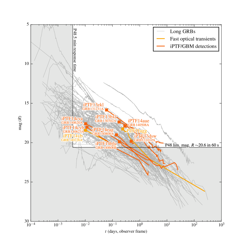
Figure 1.— Optical light curves of Fermi—iPTF afterglows to date. The light curves of the eight iPTF/GBM bursts are shown in red. For comparison, the gray lines show a comprehensive sample of long GRB optical light curves from Cenko et al. (2009), Kann et al. (2010), Perley et al. (2014d), and D. A. Kann (2015, private communication). The white area outside of the light–gray shading illustrates the range of GRB afterglows that are accessible given a half–hour cadence and the P48’s 60 s limiting magnitude of $R=20.6$. The two light curves shown in blue are other related iPTF transients. The first is PTF11agg, an afterglow–like transient with no detected gamma–ray emission (Cenko et al., 2013b). The second is GRB 140226A/iPTF14yb, reported initially by iPTF from its optical afterglow (Cenko et al. 2014; Cenko et al., in preparation), and later by IPN from its gamma-ray emission (Hurley et al., 2014b).

To date, we have successfully followed up 35 Fermi GBM bursts and detected eight optical afterglows. The detections are listed in Table 2, and all of the P48 tilings are listed in Table 3. Figure 5 shows the GBM localizations and P48 tilings for the detected bursts. In Figure 1, the light curves are shown in the context of a comprehensive sample of long GRB afterglows compiled by D. A. Kann (2015, private communication).

Table 2GBM–iPTF Detections

		R.A.	Decl.	Gal.		$E_{\mathrm{peak}}$		$E_{\gamma,\mathrm{iso}}$
GRB	OT	(J2000)	(J2000)	Lat.	$z$	(keV, rest)		($10^{52}$ erg, rest)		$T_{90}$ (s)		$m_{R}(t_{\mathrm{P48}})\tablenotemark{d}$
GRB 130702A	iPTF13bxl	14h29m15s	+15$\arcdeg$46$\arcmin$26$\arcsec$	65$\arcdeg$	0.145	18$\pm$	3	$<$0.065$\pm$	0.001	58.9$\pm$	6.2	17.38
GRB 131011A	iPTF13dsw	02h10m06s	-4$\arcdeg$24$\arcmin$40$\arcsec$	-61$\arcdeg$	1.874	625$\pm$	92	14.606$\pm$	1.256	77.1$\pm$	3	19.83
GRB 131231A	iPTF13ekl	00h42m22s	-1$\arcdeg$39$\arcmin$11$\arcsec$	-64$\arcdeg$	0.6419	291$\pm$	6	23.015$\pm$	0.278	31.2$\pm$	0.6	15.85
GRB 140508A	iPTF14aue	17h01m52s	+46$\arcdeg$46$\arcmin$50$\arcsec$	38$\arcdeg$	1.03	534$\pm$	28	24.529$\pm$	0.86	44.3$\pm$	0.2	17.89
GRB 140606B	iPTF14bfu	21h52m30s	+32$\arcdeg$00$\arcmin$51$\arcsec$	-17$\arcdeg$	0.384	801$\pm$	182	0.468$\pm$	0.04	22.8$\pm$	2.1	19.89
GRB 140620A	iPTF14cva	18h47m29s	+49$\arcdeg$43$\arcmin$52$\arcsec$	21$\arcdeg$	2.04	387$\pm$	34	7.280$\pm$	0.372	45.8$\pm$	12.1	17.60
GRB 140623A	iPTF14cyb	15h01m53s	+81$\arcdeg$11$\arcmin$29$\arcsec$	34$\arcdeg$	1.92	834$\pm$	317	3.580$\pm$	0.398	114.7$\pm$	9.2	18.04
GRB 140808A	iPTF14eag	14h44m53s	+49$\arcdeg$12$\arcmin$51$\arcsec$	59$\arcdeg$	3.29	503$\pm$	35	8.714$\pm$	0.596	4.5$\pm$	0.4	19.01

Table 3Log of P48 Tilings for Fermi GBM Bursts

		GBM		$t_{\mathrm{P48}}$	P48
	GRB Time	Fluence		$-t_{\mathrm{burst}}$	Area	Prob.
	2013 Jun 28 20:37:57	10.0$\pm$	0.1	10.02	73	32%
$\rightarrow$	2013 Jul 02 00:05:20	57.0$\pm$	1.2	4.20	74	38%
	2013 Aug 28 07:19:56	372.0$\pm$	0.6	20.28	74	64%
	2013 Sep 24 06:06:45	37.0$\pm$	0.6	23.24	74	28%
	2013 Oct 06 20:09:48	18.0$\pm$	0.6	15.26	74	18%
$\rightarrow$	2013 Oct 11 17:47:30	89.0$\pm$	0.6	11.56	73	54%
	2013 Nov 08 00:34:39	28.0$\pm$	0.5	4.69	73	37%
	2013 Nov 10 08:56:58	33.0$\pm$	0.3	17.47	73	44%
	2013 Nov 25 16:32:47	5.5$\pm$	0.3	11.72	95	26%
	2013 Nov 26 03:54:06	17.0$\pm$	0.3	6.94	109	59%
	2013 Nov 27 14:12:14	385.0$\pm$	1.4	13.46	60	50%
	2013 Dec 30 19:24:06	41.0$\pm$	0.4	7.22	80	38%
$\rightarrow$	2013 Dec 31 04:45:12	1519.0$\pm$	1.2	1.37	30	32%
	2014 Jan 04 17:32:00	333.0$\pm$	0.6	18.57	15	11%
	2014 Jan 05 01:32:57	6.4$\pm$	0.1	7.63	74	22%
	2014 Jan 22 14:19:44	9.1$\pm$	0.5	11.97	75	34%
	2014 Feb 11 02:10:41	7.4$\pm$	0.3	1.77	44	19%
	2014 Feb 19 19:46:32	28.0$\pm$	0.5	7.01	71	14%
	2014 Feb 24 18:55:20	24.0$\pm$	0.6	7.90	72	30%
	2014 Mar 11 14:49:13	40.0$\pm$	1.2	12.18	73	54%
	2014 Mar 19 23:08:30	71.0$\pm$	0.3	3.88	74	48%
	2014 Apr 04 04:06:48	82.0$\pm$	0.2	0.11	109	69%
	2014 Apr 29 23:24:42	6.2$\pm$	0.2	10.99	74	15%
$\rightarrow$	2014 May 08 03:03:55	614.0$\pm$	1.2	6.68	73	67%
	2014 May 17 19:31:18	45.0$\pm$	0.4	8.60	95	69%
	2014 May 19 01:01:45	39.0$\pm$	0.5	4.42	73	41%
$\rightarrow$	2014 Jun 06 03:11:52	76.0$\pm$	0.4	4.08	74	56%
	2014 Jun 08 17:07:11	19.0$\pm$	0.6	11.20	73	49%
$\rightarrow$	2014 Jun 20 05:15:28	61.0$\pm$	0.6	0.17	147	59%
$\rightarrow$	2014 Jun 23 05:22:07	61.0$\pm$	0.6	0.18	74	4%
	2014 Jun 28 16:53:19	18.0$\pm$	1.0	16.16	76	20%
	2014 Jul 16 07:20:13	2.4$\pm$	0.3	0.17	74	28%
	2014 Jul 29 00:36:54	81.0$\pm$	0.7	3.43	73	65%
	2014 Aug 07 11:59:33	13.0$\pm$	0.1	15.88	73	54%
$\rightarrow$	2014 Aug 08 00:54:01	32.0$\pm$	0.3	3.25	95	69%

The outcome of an individual afterglow search is largely determined by two factors: how much probability is contained within the P48 footprints, and how bright the afterglow is at the time of the observations (see Figure 2). We calculate the expected success rate as follows. For each burst, we find the prior probability that the position is contained within the P48 fields that we observed. We then compute the fraction of afterglows from Kann’s sample (which has a mean and standard deviation of $22\pm 2$ mag at $t=1$ day) that are brighter than $R=20.6$ mag at the same age as when the P48 observations started. The product of these two numbers is the prior probability of detection for that burst. By summing over all of the iPTF/GBM bursts, we obtain the expected number of detections. Within 95% confidence bootstrap error bars, we find an expected 5.5—8.5 detections, or a success rate of 16%—24%. This is consistent with the actual success rate of 23%.

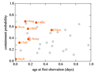
Figure 2.— Prior probability of containing the burst’s location within the P48 fields vs. age of the burst at the beginning of P48 observations. Afterglow detections are shown in orange, and non–detections are shown in gray.

This suggests that the success rate is currently limited by the survey area and the response time (dictated by sky position and weather). We could increase the success rate by decreasing the maximum time since trigger at which we begin follow–up. We could increase the success rate without adversely affecting the number of detections by simply searching a greater area for coarsely localized events.

Fig. Set3. Light curves and SEDs

Figure 3.— Light curves and SEDs of GBM—iPTF afterglows; GRB 130702A / iPTF13bxl is shown here in the print version.
(An extended version of this figure set is available in the online journal.)

Over the next few sections, we summarize the observations and general physical interpretation of all of the GBM—iPTF afterglows detected to date. Figure 3 shows the light curves and SEDs spanning X–ray, UV, optical, IR, and radio frequencies. Table 4 contains a log of our spectroscopic observations. Table 5 lists a selection of ultraviolet, optical, and infrared observations, including all of our P48 and P60 observations. Table 6 lists all of our radio detections.

Table 4Log of Spectroscopic Observations

Date	Telescope	Instrument	Wavelengths (Å)	Lines	References
GRB 131011A/iPTF13dsw
2013 Oct 12 08:56	Gemini South	GMOS	5100–9300	none	Kasliwal et al. (2013)
2013 Oct 13 03:59	ESO/VLT UT3	X-shooter	3100–5560	Ly$\alpha$, Si II, C II, C IV, Al II	Rau et al. (2013)
$\cdots$	$\cdots$	$\cdots$	5550–10050	Fe II, Mg II	$\cdots$
GRB 131231A/iPTF13ekl
2014 Jan 01 02:15	Gemini South	GMOS	6000–10000	[O II], [O III], Ca II H+K	Cucchiara (2014)
GRB 140508A/iPTF14aue
2014 May 08 18:55	HCT	HFOSC	3800–8400	Fe II, Mg II	Bhalerao & Sahu (2014)
2014 May 09 06:33	APO	DIS	3200–9800	none	none
GRB 140606B/iPTF14bfu
2014 Jun 07 19:16	Keck II	DEIMOS	4500–9600	[O II], [O III], H$\alpha$, Ca II H+K	Perley et al. (2014a)
GRB 140620A/iPTF14cva
2014 Jun 20 14:00	Gemini North	GMOS	5090–9300	Mg I, Mg II, Fe II, Al II, Si II, Si II∗	Kasliwal et al. (2014)
$\cdots$	$\cdots$	$\cdots$	4000–6600	$\cdots$	$\cdots$
GRB 140623A/iPTF14cyb
2014 Jun 23 08:10	Gemini North	GMOS	4000–6600	Mg II, Fe II, Al II, Si II, Al III, C I, C IV	Bhalerao et al. (2014)
GRB 140808A/iPTF14eag
2014 Aug 08 21:43	GTC	OSIRIS	3630–7500	DLA, S II, Si II, O I, C II, Si IV, Fe II, Al II, C IV	Gorosabel et al. (2014a)

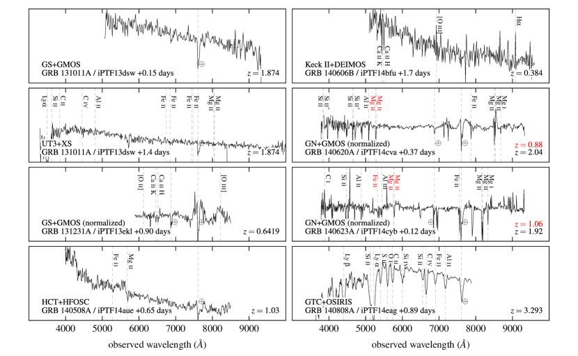
Figure 4.— Afterglow spectra. The horizontal axis shows wavelength in vacuum in the observer frame, and the vertical axis shows scaled flux. Lines at the redshift of the putative host are labeled in black; lines corresponding to any intervening absorbing systems are labeled in red. Note that in cases where one or fewer lines are discernible in our spectra, the redshifts have been reported in GCNs by other groups.

Table 5Optical Observations of GBM–iPTF Afterglows

Date (mid)	Inst.	$\Delta t$	Mag.
GRB 130702A/iPTF13bxl
2013 Jul 02 04:18	P48	0.18	$R$	$=$	17.38 $\,\pm\,$	0.04
2013 Jul 02 05:10	P48	0.21	$R$	$=$	17.52 $\,\pm\,$	0.04
2013 Jul 03 04:13	P60	1.17	$g$	$=$	18.80 $\,\pm\,$	0.04
2013 Jul 03 04:15	P60	1.17	$i$	$=$	18.42 $\,\pm\,$	0.04
2013 Jul 03 06:16	P60	1.26	$i$	$=$	18.56 $\,\pm\,$	0.06
2013 Jul 03 06:17	P60	1.26	$r$	$=$	18.66 $\,\pm\,$	0.05
2013 Jul 03 06:20	P60	1.26	$g$	$=$	18.86 $\,\pm\,$	0.04

Note. — A machine readable version of this table is available in the online journal.

Table 6Radio Observations of GBM–iPTF Afterglows

Date (Start)	Inst.	$\Delta t$	Flux Density
GRB 130702A/iPTF13bxl
2013 Jul 04	CARMA	2	$f_{\nu}(93)$	$=$	1580	$\pm$	330
2013 Jul 04	VLA	2.3	$f_{\nu}(5.1)$	$=$	1490	$\pm$	75
2013 Jul 04	VLA	2.3	$f_{\nu}(7.1)$	$=$	1600	$\pm$	81
2013 Jul 05	CARMA	3.1	$f_{\nu}(93)$	$=$	1850	$\pm$	690
2013 Jul 06	CARMA	4.1	$f_{\nu}(93)$	$=$	1090	$\pm$	350
2013 Jul 08	CARMA	6.1	$f_{\nu}(93)$	$=$	1440	$\pm$	260
2013 Jul 08	CARMA	7	$f_{\nu}(93)$	$=$	1160	$\pm$	320
2013 Jul 14	CARMA	12	$f_{\nu}(93)$	$=$	900	$\pm$	230
2013 Jul 15	CARMA	13	$f_{\nu}(93)$	$=$	1550	$\pm$	590
2013 Jul 24	CARMA	22	$f_{\nu}(93)$	$=$	1430	$\pm$	480
2013 Jul 25	CARMA	23	$f_{\nu}(93)$	$<$	1890
2013 Aug 12	CARMA	41	$f_{\nu}(93)$	$=$	450	$\pm$	210

Note. — A machine readable version of this table is available in the online journal.

3.1. GRB 130702A/iPTF13bxl

This is the first GBM burst whose afterglow we discovered with iPTF (Singer et al., 2013b), indeed the first afterglow ever to be pinpointed based solely on a Fermi GBM localization. It is also the lowest–redshift GRB in our sample, so it has the richest and most densely sampled broadband afterglow data. It has two other major distinctions: its associated SN (SN 2013dx, Schulze et al. 2013; Pozanenko et al. 2013; Cenko et al. 2013a; D’Elia et al. 2013) was detected spectroscopically, and its prompt energetics are intermediate between low–luminosity s and standard cosmic bursts (see below).

Based on the Fermi GBM ground localization with an error radius of $4\arcdeg$, we imaged 10 fields twice with the P48 at $\Delta t=t-t_{\mathrm{GBM}}=4.2$ hr after the burst. We scheduled P60 imaging and P200 spectroscopy for three significantly varying sources. Of the three, iPTF13bxl showed the clearest evidence of fading in the P48 images. Its spectrum at $\Delta t=1.2$ days consisted of a featureless blue continuum. We triggered Swift, which found a bright X-ray source at the position of iPTF13bxl (Singer et al., 2013c; D’Avanzo et al., 2013). Shortly after we issued our GCN circular (Singer et al., 2013c), Cheung et al. (2013) announced that the burst had entered the FOV of LAT at $\Delta t=250$ s. The LAT error circle had a radius of $0\fdg 5$, and its center was $0\fdg 8$ from iPTF13bxl. An IPN triangulation with MESSENGER (GRNS), INTEGRAL (SPI–ACS), Fermi–GBM, and Konus–Wind (Hurley et al., 2013) yielded a $0\fdg 46$–wide annulus that was also consistent with the OT.

The afterglow’s position is $0\farcs 6$ from an $R=23.01$ mag source that is just barely discernible in the P48 reference images. A spectrum from NOT+ALFOSC (Leloudas et al., 2013) determined a redshift of $z=0.145$ for a galaxy $7\farcs 6$ to the south of iPTF13bxl. At $\Delta t=2.0$ days, we obtained a Magellan+IMACS spectrum (Mulchaey et al., 2013) and found weak emission lines at the location of the afterglow that we interpreted as H$\alpha$ and [O III] at the same redshift. Kelly et al. (2013) characterized the burst’s host environment in detail and concluded that it exploded in a dwarf satellite galaxy.

Joining the two P48 observations at $\Delta t<1$ day to the late–time P60 light curve requires a break at $\Delta t=1.17\pm 0.09$ days, with slopes $\alpha_{\mathrm{O},1}=0.57\pm 0.03$ and $\alpha_{\mathrm{O},2}=1.05\pm 0.03$ before and after the break, respectively. The XRT light–curve begins just prior to this apparent break and seems to follow the late–time optical decay (until the SN begins to dominate at $\Delta t=5$ days), although the automated Swift light curve analysis (Evans et al., 2009) also suggests a possible X–ray break with about the same time and slopes. This hints at an achromatic break, normally a signature of a jet. However, the late slope and the change in slope are both unusually shallow for a jet break. Furthermore, the radio light curve does not exhibit a break. The change in slope is also a little too large for cooling frequency crossing the band (for which one would expect $\Delta\alpha=1/4$). An energy injection or a structured jet model may provide a better fit (Panaitescu, 2005).

Late–time $\Delta t>1$ day observations include several P60 $gri$ observations, three RATIR $r^{\prime}i^{\prime}ZYJH$ epochs, an extensive Swift XRT and UVOT light curve, and radio observations with VLA and CARMA (although of the VLA data, we only have access to the first observation). The optical and X-ray spectral slopes are similar, $\beta_{\mathrm{O}}=0.7\pm 0.1$ and $\beta_{\mathrm{X}}=0.8\pm 0.1$. An SED at $2<\Delta t<2.3$ days is well explained by the standard external shock model (Sari et al., 1998) in the slow cooling regime, with $\nu_{m}$ lying between the VLA and CARMA frequencies and $\nu_{c}$ in the optical. This fit requires a relatively flat electron spectrum, $dn_{\mathrm{e}}/d\gamma_{\mathrm{e}}\propto{\gamma_{\mathrm{e}}}^{-p}$ with $p\approx 1.6$, cut off at high energies. Applying the relevant closure relations (for the case of $1<p<2$, see Dai & Cheng 2001) to $\alpha_{X}$ and $\beta_{X}$ permits either an ISM or wind environment.

Our late–time spectroscopy and analysis of the SN will be published separately (S. B. Cenko et al. 2015, in preparation).

3.2. GRB 131011A/iPTF13dsw

We started P48 observations of Fermi trigger 403206457 (Jenke, 2013) about 11.6 hr after the burst. The optical transient iPTF13dsw (Kasliwal et al., 2013) faded from $R=19.7$ mag to $R=20.2$ mag from 11.6 to 14.3 hr. The latest pre–trigger image on 2013 September 25 had no source at this location to a limit of $R>20.6$ mag. The optical transient continued to fade as it was monitored by several facilities (Xu et al., 2013a, c; Perley et al., 2013; Sudilovsky et al., 2013; Volnova et al., 2013).

At 15.1 hr after the burst, we obtained a spectrum of iPTF13dsw with the Gemini Multi-object Spectrograph (GMOS) on the Gemini—South telescope. GMOS was configured with the R400 grating with a central wavelength of 7200 Å and the 1″slit, providing coverage over the wavelength range of 5100—9300 Å with a resolution of $\approx 3$ Å. No prominent features were detected over this bandpass, while the spectrum had a typical SNR of $\approx 3$—4 per 1.4 Å pixel. Rau et al. (2013) observed the optical transient with the X–Shooter instrument on the ESO 8.2–m VLT. In their spectrum extending from $\sim$3000 to $\sim 24000$Å, they identified several weak absorption lines from which they derived a redshift of $z=1.874$. Both spectra are shown in Figure 4.

The source was detected by Swift XRT (Page, 2013), but with insufficient photons for spectral analysis. The source was observed with ATCA, but no radio emission was detected. Largely because in our sample this is the oldest afterglow at the time of discovery, there are not enough broadband data to constrain the blast wave physics.

3.3. GRB 131231A/iPTF13ekl

GRB 131231A was detected by Fermi LAT (Sonbas et al., 2013) and GBM (Jenke & Xiong, 2014), with photons of energies up to 9.7 GeV. Xu et al. (2013b) observed the LAT error circle with the 1–m telescope at Mt. Nanshan, Xinjiang, China. At 7.9 hr after the burst, they detected a single $R=\sim 17.6$ mag source that was not present in SDSS images. At 17.3 hr after the burst, Malesani et al. (2013) observed the afterglow candidate with the MOSaic CAmera (MOSCA) on the 2.56–m Nordic Optical Telescope (NOT). The source had faded to $R=18.6$.

Although we had imaged 10 P48 fields shortly after the Fermi trigger (Singer et al., 2013a), due to the short visibility window at Palomar we were only able to obtain one epoch. At 1.45 hr after the burst, we detected an $R=15.7$ mag optical transient iPTF13ekl at the position of the Nanshan candidate. Though our single detection of iPTF13ekl could not by itself rule out that the source was a moving solar system object, the Nanshan detection at 6.46 hr, fitting a decay with a power–law index of $\alpha=1.03$, was strong evidence that the transient was the optical afterglow of GRB 131231A.

On January 1.09 UT (21.5 hr after the trigger), we observed the afterglow with Gemini South using the GMOS camera (Hook et al., 2004) in Nod&Shuffle mode: we obtained 32 dithered observations of 30 s each at an average airmass of 2. We analyzed this data set using the dedicated GEMINI package under the IRAF environment and extracted the 1-dimensional spectrum using the APALL task. We determined the redshift of the GRB, based on the simultaneous identification of forbidden nebular emission lines ([O II], [O III]) and absorption features (CaH&K) at the same redshift of $z=0.6419$. In Figure 4, we show the normalized spectrum.

The source was also detected by Swift XRT (Mangano et al., 2014b) and UVOT (Holland & Mangano, 2014), as well as CARMA (Perley, 2014).

With only the millimeter, optical, and X–ray observations, the SED is highly degenerate. Contributing to the degeneracy, the X–ray and optical observations appear to fall on the same power–law segment. It is consistent with either fast or slow cooling if the greater of $\nu_{c}$ or $\nu_{m}$ is near the optical, assuming a flat electron distribution with $p\sim 1.5$. It is also consistent with slow cooling if $\nu_{c}$ is above the X–ray band and $p\sim 2.6$.

3.4. GRB 140508A/iPTF14aue

This burst was detected by Fermi GBM and INTEGRAL SPI–ACS (Yu & Goldstein, 2014), as well as by Konus–Wind, Mars Odyssey (not included in the GCN circular), Swift BAT (outside the coded FOV), and MESSENGER, yielding a $1\fdg 5\times 12\arcmin$ IPN error box (Hurley et al., 2014c).

Due to poor weather early in the night, P48 observations started 6.7 hr after the trigger (Singer et al., 2014a). We found one optical transient candidate within the IPN triangulation, iPTF14aue, which faded from $r=17.89\pm 0.01$ mag with a power–law fit of $\alpha=1.12\pm 0.1$ over a timescale of 1.5 hr.

We triggered a Swift TOO. From 0.8 to 8.1 days after the trigger, Swift XRT detected a coincident X–ray source that faded with a power law $\alpha=1.48\;(+0.15,-0.14)$ (Amaral-Rogers, 2014a, b). The source was also detected by Swift UVOT (Marshall & Amarel-Rogers, 2014).

Moskvitin et al. (2014) obtained a 20–minute, 3800—7200 Å spectrum of iPTF14aue with the 6–m BTA telescope in Zelenchukskaia. Exhibiting no absorption features, this established an upper limit of $z<2.1$. Malesani et al. (2014) used the Andalucia Faint Object Spectrograph and Camera (ALFOSC) on NOT to get an 1800 s spectrum spanning 3200—9100 Å, and found several absorption features at redshift $z=1.03$. Consistent redshifts were reported by Wiersema et al. (2014) with the ACAM instrument on the 4.2–m William Herschel Telescope and by Bhalerao & Sahu (2014) with Himalaya Faint Object Spectrograph and Camera (HFOSC) on the 2–m HCT. This last spectrum is shown in Figure 4.

Due to the brightness of the optical transient, optical photometry was available from several facilities up to 4.5 days after the burst (Gorosabel et al., 2014b; Moskvitin et al., 2014; Malesani et al., 2014; Masi, 2014; Butler et al., 2014b, a; Fujiwara et al., 2014; Volnova et al., 2014a).

Horesh et al. (2014) detected the source with VLA 5.2 days after the Fermi trigger, at 6.1 GHz ($C$ band) and at 22 GHz ($K$ band). A broadband SED constructed from P60 and XRT data from around this time is consistent with $p\approx 2$. Because $p$ is not distinguishable from 2, we cannot discriminate between fast and slow cooling based on this one time slice. However, given the late time of this observation, the slow cooling interpretation is more likely, putting $\nu_{m}$ between the radio and optical bands and $\nu_{c}$ between the optical and X–ray. Because the VLA light curve is decreasing with time, an interstellar medium (ISM) circumburst density profile is favored.

3.5. GRB 140606B/iPTF14bfu

Fermi trigger 423717114 (Burns, 2014) was observable from Palomar for several hours, starting about 4.3 hr after the time of the burst. Based on the final GBM localization, we searched ten P48 fields and found several plausible optical transient candidates (Singer et al., 2014c).

iPTF14bfu had no previous detections in iPTF between 2013 May 23 and October 13. Its position was outside the SDSS survey footprint, but it had no plausible host associations in VizieR (Ochsenbein et al., 2000). From 4.3 to 5.5 hr after the burst, it faded from $R=19.89\pm 0.10$ to $20.32\pm 0.14$ mag, fitting a power law of $\alpha=-1.6\pm 0.7$ relative to the time of the GBM trigger. iPTF14bfw ($R=19.96\pm 0.06$ mag) was coincident with an $r=21.27$ galaxy in SDSS DR10 and displayed no statistically significant photometric variation over the course of our P48 observations. iPTF14bgc ($R=18.44\pm 0.02$ mag) was coincident with an $R=21.07\pm 0.08$ mag point source in our co–added reference image composed of exposures from 2013 July 31 through September 24. iPTF14bga ($R=19.75\pm 0.06$ mag) was likewise coincident with a $R=20.42\pm 0.17$ mag point source in our reference image composed of exposures from 2011 July 29 through October 20.

On the following night, we observed all four candidates again with P48 and P60 (Perley & Singer, 2014). iPTF14bfw and iPTF14bga had not faded relative to the previous night. iPTF14bgc had faded to $R=20.68\pm 0.21$ mag, consistent with the counterpart in our reference images but significantly fainter than the previous night. A power–law fit to the decay gave a temporal index of $\alpha=-1.1\pm 0.1$, entirely consistent with typical GRB afterglows. iPTF14bfu was not detected in our P48 images to a limiting magnitude of $R<21.1$, but it was detected in stacked P60 images ($r=21.1\pm 0.2$), consistent with a power law of $\alpha\sim-0.5$.

An IPN triangulation from Fermi, Konus—Wind, and MESSENGER yielded a long, slender $14\fdg 18\times 0\fdg 414$ error box that contained iPTF14bfu and iPTF14bfw (Hurley et al., 2014d).

We obtained two 900 s spectra with the DEIMOS spectrograph on the Keck II 10 m telescope (Perley et al., 2014a). On a blue continuum, we found [O II], [O III], and H $\alpha$ emission features and Ca II absorption features, at a common redshift of $z=0.384$. A galaxy offset by $\sim 2\arcsec$ along the slit showed the same emission lines at the same redshift.

Swift XRT observed the location of iPTF14bfu for a total of 9 ks from 2.1 to 9.3 days after the GBM trigger, and found a source that faded with a power–law fit of $\alpha=-1.0\;(+0.7,-0.6)$ (Mangano et al., 2014a; Mangano & Burrows, 2014; Mangano, 2014).

At 18.4 days after the trigger, we obtained a 1200 s spectrum of iPTF14bfu with the Low Resolution Imaging Spectrometer (LRIS) on the Keck I 10–meter telescope (Perley et al., 2014b). The spectrum had developed broad emission features. A comparison using Superfit (Howell et al., 2005) showed a good match to SN 1998bw near maximum light, indicating that the source had evolved into an  Ic–BL. Our late–time photometry and spectroscopy will published separately (Cano et al., 2015).

Although there were three radio detections of GRB 140606B, only during the first CARMA detection does the optical emission appear to be dominated by the afterglow. We can construct an SED around this time using nearly coeval DCT and XRT data. Because of the faintness of the X–ray afterglow, the spectral slopes $\beta_{\mathrm{X}}$ and $\beta_{\mathrm{OX}}$ are only weakly determined. As a result, there is a degeneracy between two plausible fits. The first has $\nu_{m}$ anywhere below the CARMA band, $\nu_{c}$ just below the X–rays, and $p\approx 2$. The second has $\nu_{m}$ just above the radio and $\nu_{c}$ in the middle of the XRT band, with $p\approx 2.2$.

The early P48 observations do not connect smoothly with the P60 and DCT observations from $\Delta t=1$ to 4 days. This may indicate a steep—shallow—steep time evolution requiring late–time energy injection, or may just indicate that the afterglow is contaminated by light from the host galaxy or the SN at relatively early times.

3.6. GRB 140620A/iPTF14cva

This burst is distinctive in our sample for two reasons. First, it is the earliest afterglow detection in the iPTF sample at $\Delta t=0.25$ hr. Second, its broadband SED is not clearly explainable by the standard forward shock model.

Fermi trigger 424934131 (Fitzpatrick & Connaughton, 2014) was observable from Palomar for about 6 hr from the time of the burst. Based on the ground localization, we started observing ten P48 fields about 10 minutes after the trigger. Based on the final localization, we added 10 more fields, for a total of 20, about an hour after the trigger.

The candidate iPTF14cva (Kasliwal et al., 2014) was contained within one of the early 10 fields. From 14.9 to 87.2 minutes after the trigger, the candidate faded from $R=17.60\pm 0.01$ to $18.80\pm 0.02$ mag, consistent with a somewhat slow power law of $\alpha=0.62\pm 0.01$.

We observed the candidate with GMOS on the 8–m Gemini North telescope. Starting 8.8 hr after the trigger, we obtained two 900 s spectra extending from 4000 to 9300 Å. We detected Mg II and Fe II absorption lines at $z=0.88$ and many absorption features at a common redshift of $z=2.04$. The lack of Ly$\alpha$ absorption implied an upper limit of $z\sim 2.3$ and suggested that $z=2.04$ was the redshift of the source.

We triggered Swift and VLA follow–up. In a 3 ks exposure starting 10.4 hr after the Fermi trigger, Swift XRT detected an X–ray source with a count rate of $1.2\times 10^{-1}$ counts s^-1 (De Pasquale, 2014b). Over the next four days of Swift observations, the X-ray source faded with a slope $\alpha=1.32\pm 0.16$ (De Pasquale, 2014a). A fading source was also detected by Swift UVOT (Siegel & De Pasquale, 2014).

The source was detected by VLA on June 23 at 6.1 GHz ($C$ band) at $108\pm 15$ $\mu$Jy and at 22 GHz ($K$ band) at $62\pm 15$ $\mu$Jy. On June 30, there was a marginal detection in $C$ band with $48\pm 12$ $\mu$Jy and no detection in $K$ band with a noise level of 15 $\mu$Jy rms.

The optical transient was also observed in $R$ band by the Konkoly Observatory (Kelemen, 2014) and the 1–m telescope at the Tien Shan Astronomical Observatory (Volnova et al., 2014b).

The SED of this afterglow cannot be explained by a standard forward shock model. If we place the peak frequency near the radio band, the optical and X–ray fluxes are drastically underpredicted, whereas if we place the peak frequency between the optical and X–ray bands, we miss the radio observations by orders of magnitude. This seems to require an additional component. One possibility is that there is a forward shock peak in the UV and a reverse shock peak at low frequencies (similar to GRB 130427A; see Laskar et al. 2013; Perley et al. 2014d). Another possibility is that there is an inverse Compton peak in the UV (similar to GRB 120326A; Urata et al. 2014).

3.7. GRB 140623A/iPTF14cyb

Fermi trigger 425193729 (von Kienlin, 2014) was observable from Palomar for about 6 hr from the time of the burst. Based on the ground localization, we started imaging 10 fields 11 minutes after the trigger. The final Fermi localization, which was avilable 2.6 hr later, shifted by 13$\fdg$4. Due to the large change in the localization, we calculated only a 4% chance that the source was contained within the P48 fields.

Candidate iPTF14cyb (Kasliwal et al., 2014), situated at an extreme edge of the P48 tiling, was within the 1$\sigma$ confidence region for both the ground and final localizations. From 16 to 83 minutes after the trigger, the source faded from $R=18.04\pm 0.01$ to $19.69\pm 0.06$ mag, consistent with a power-law decay with an index $\alpha=0.94\pm 0.03$.

Starting 2.8 hr after the trigger, we obtained two 900 s GMOS spectra extending from 4000 to 9300 Å. We detected Mg II and Fe II absorption lines at $z=1.06$ and many absorption features at $z=1.92$. The lack of Ly$\alpha$ absorption implied that this was the redshift of the burst.

We triggered Swift, VLA, and CARMA follow–up. In a 3 ks exposure starting 10.7 hr after the burst, Swift XRT detected an uncataloged X–ray source with a count rate of $(2.2\pm 0.6)\times 10^{-3}$ counts s^-1 (D’Elia et al., 2014). By 79 hr after the trigger, the source was no longer detected in a 5 ks exposure (D’Elia & Izzo, 2014). No radio source was detected with VLA in $C$ band (6.1 GHz) to an rms level of 17 $\mu$Jy, or in $K$ band (22 GHz) to an rms level of 18 $\mu$Jy.

Because of the lack of radio detections and the extreme faintness of the X–ray afterglow, the broadband behavior of the afterglow does not constrain the shock physics.

3.8. GRB 140808A/iPTF14eag

Fermi trigger 429152043 (Zhang, 2014) was observable from Palomar about 3 hr after the burst. We imaged 13 fields with P48 and found one promising optical transient. iPTF14eag was situated on the extreme edge of one of the P48 tiles that was just outside the GBM 1$\sigma$ contour. It faded from $R=18.91\pm 0.06$ to $19.29\pm 0.10$ mag from 3.35 to 4.91 hr after the trigger and had no archival counterparts in SDSS or in our own reference images.

Due to Hurricane Iselle, we were unable to use our TOO programs on Keck or Gemini North. We requested photometric confirmation of the fading from HCT (Sahu et al., 2014), submitted a Swift TOO, and sent our GCN circular (Singer et al., 2014b) to encourage others to obtain a spectrum.

Swift observed the position of iPTF14eag from 11.6 to 14.4 hr after the burst (Page et al., 2014). An X-ray source was detected with a count rate of $1.5\times 10^{-2}$ counts s^-1. In a second observation starting 62.2 hr after the trigger (Page & Cenko, 2014), the source had faded to below $2.46\times 10^{-3}$ counts s^-1. No source was detected by UVOT (Oates & Cenko, 2014).

We obtained a spectrum with the OSIRIS instrument (Cepa et al., 2000) on Gran Telescopio Canarias (GTC) in $4\times 900$ s exposures with a mean epoch of 21.340 hr after the burst. We used the R1000B grism and a 1” slit, with a resolution of R 1000. We determined a redshift of 3.293 (improved from the one given by Gorosabel et al. 2014a) through the identification of strong absorption features. The flux–calibrated spectrum is shown in Figure 4.

The source was detected in radio with VLA (Corsi & Horesh, 2014) and AMI (Anderson et al., 2014a). The broadband SED around the time of the VLA detection broadly fits a forward shock model but is poorly constrained due to the lack of a contemporaneous X–ray detection. The spectral slope between the two VLA bands is somewhat steeper than the standard low–frequency value of $\beta=-1/3$, possibly indicating that the radio emission is self–absorbed. We obtained 14 AMI observations every 2 or 3 days from 2014 August 8 until 2014 September 12. Observations were 2—4 hr in duration. AMI first detected the afterglow 4.6 days post-burst. The AMI light curve peaked $\sim$10.6 days post–burst at 15.7 GHz, which is characteristic of forward shock emission at radio wavelengths (Chandra & Frail, 2012).

A peculiar feature of the optical light curve is that the P60 $r$- and $i$–band observations at $\Delta t\approx 2$ days appears to be inverted, with a rising rather than falling spectral shape, compared to the earlier P60 photometry at $\Delta t\approx 1$ day. However, this feature is within the error bars and may be merely a statistical fluctuation.

This is the highest–redshift burst in our sample and also had the weakest prompt emission in terms of the fluence observed by GBM.

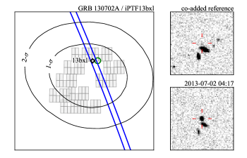
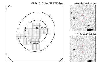
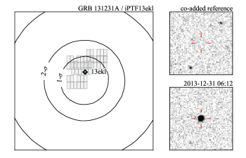
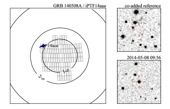
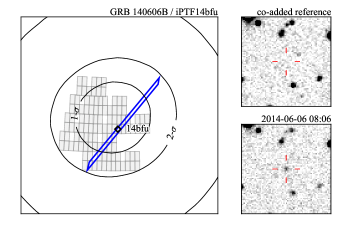
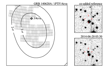
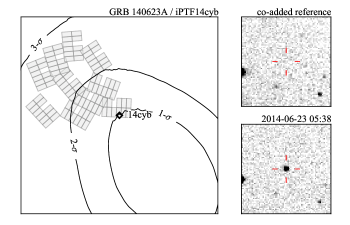
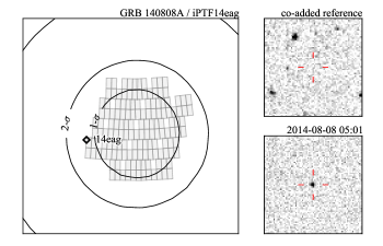
Figure 5.— Gamma–ray localizations, P48 tiles, and discovery images for the GBM—iPTF afterglows. The Fermi GBM 1- and 2–$\sigma$ regions are shown as black contour lines, the P48 tiles as gray rectangles, the 3$\sigma$ IPN triangulations in blue (when available), and the LAT 1$\sigma$ error circles in green (when available). The positions of the optical transients are marked with black diamonds.

4. The Population in Context

4.1. Selection Effects

First, we investigate the properties of the subset of GBM bursts followed up by iPTF compared to the GBM bursts as a whole. It is known that, on average, GRBs with larger prompt fluences have brighter optical afterglows, though the correlation is very weak (Nysewander et al., 2009). In Figure 6, we plot the fluence in the 10—1000 keV band and 1–$\sigma$ localization radius of all GBM bursts from the beginning of our experiment, retrieved from the Fermi GBM Burst Catalog at HEASARC. As expected, there is a weak but clearly discernible correlation between fluence and radius, $F\propto r^{-1.3}$, with a Pearson correlation coefficient of $R=0.64$. The subset of bursts that we followed up spans a wide range in fluence and error radii up to $\sim 10\arcdeg$. The bursts for which we detected optical afterglows are preferentially brighter, with the faintest burst having a fluence as low as $3\times 10^{-6}$ erg cm^-2. There are some bright ($>3\times 10^{-5}$ erg cm^-2) and well–confined ($<1.8\arcdeg$) events for which we did not find afterglows: those at 2013 August 28 07:19:56, 2013 November 27 14:12:14, and 2014 January 04 17:32:00 (see Table 3). However, these non–detections are not constraining given their ages of 20.28, 13.46, and 18.57 hours respectively. Conversely, there were two especially young bursts (followed up at $\Delta t=0.11$ and 0.17 hr) for which we did not detect afterglows. The non–detection of the burst at 2014 July 16 07:20:13 makes sense because we searched only 28% of the GBM localization. The non–detection on 2014 Paril 04 04:06:48, for which we observed 69% of the localization, is a little more surprising, especially given its relatively high fluence of $8\times 10^{-6}$ erg cm^-2; this is a possible candidate for a “dark GRB.” On the whole, however, we can see that (1) we have followed up bursts with a large range of error radii and fluences, (2), there is a weak preference toward detecting bursts with small error radii, and (3) the detections tend toward bursts with high fluences. Naively one might expect higher fluences to translate into lower redshifts, but the interplay between the GRB luminosity function and detector threshold greatly complicates such inferences (Butler et al., 2010).

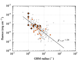
Figure 6.— Fluence and statistical error radius of GBM bursts. Orange dots mark bursts that were followed up with iPTF; black circles around orange dots mark bursts whose afterglows were detected by iPTF. The black line is a power–law fit.

Second, the rich sample of all of the GRB afterglows that we have today is undeniably the result of the success of the Swift mission. It is therefore interesting to consider how the GBM—iPTF sample is similar to or different from the Swift sample, given the differences in bandpasses and our increased reliance on the optical afterglow. In Figure 7, we plot the cumulative redshift distribution of our sample, alongside the distribution of redshifts of long GRBs detected by Swift. Indeed, we find that our sample is at lower redshifts; the former distribution lies almost entirely to the left of the latter, and the ratio of the median redshifts ($z=1.5$ versus $z=1.9$) of the two populations is about 0.75. However, with the small sample size, the difference between the two redshift distributions is not significant: a two–sample Kolmogorov—Smirnov test yields a $p$–value of 0.26, meaning that there is a 26% chance of obtaining these two empirical samples from the same underlying distribution. More GBM—iPTF events are needed to determine whether the redshift distribution is significantly different.

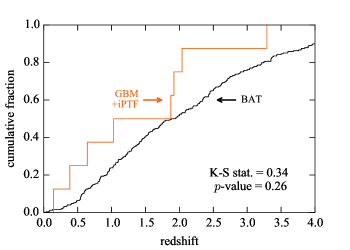
Figure 7.— Cumulative distribution of redshifts of long GRBs observed by Swift BAT (gray) and the GBM—iPTF experiment (orange).

4.2. GRBs as Standard Candles?

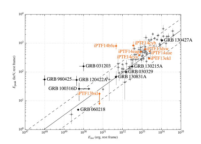
Figure 8.— Rest–frame energetics of GBM—iPTF bursts (in orange) in comparison to an illustrative sample of previous GRB—SNe (in black; includes GRB 060218/SN2006aj, Pian et al. 2006, Modjaz et al. 2006, Sollerman et al. 2006; GRB 100316D/SN2010bh, Chornock et al. 2010, Bufano et al. 2011; GRB 120422A/SN2012bz, Melandri et al. 2012, Schulze et al. 2014a; GRB 130215A/SN2013ez, Cano et al. 2014; GRB 130427A/SN2013cq, Xu et al. 2013d; and GRB 130831A/SN2013fu, Klose et al. 2013). A general long GRB sample from Amati (2006) and Amati et al. (2008, 2009) is shown in gray. The solid black line represents the Amati relation as given in Amati (2006), $E_{\mathrm{peak}}=95(E_{\gamma,\mathrm{iso}}/10^{52}\text{ erg})^{0.49}$ keV. The black dashed lines show the relation’s $1\sigma$ dispersion of $\pm 0.4$ dex.

Amati et al. (2002) pointed out a striking empirical correlation in the rest–frame prompt emission spectra of BeppoSAX GRBs, with the peak energy (in the $\nu F_{\nu}$ sense) $E_{\mathrm{peak}}$ related to the bolometric, isotropic–equivalent energy release $E_{\mathrm{iso}}$ by $E_{\mathrm{peak}}\propto{E_{\mathrm{iso}}}^{m}$. It was quickly realized that such a relation, if intrinsic to the bursts, could be used to measure the redshifts of GRBs non–spectroscopically (Atteia, 2003). As with the Phillips relation for SNe Ia (Phillips, 1993), with such a relation GRBs could serve as standardizable candles in order to measure cosmological parameters (Dai et al. 2004; Friedman & Bloom 2005; Ghirlanda et al. 2006; etc.).

However, there has been a vigorous debate about whether the Amati relation and related correlations are innate to GRBs or reflect a detector–dependent selection bias (Band & Preece, 2005; Ghirlanda et al., 2005; Nakar & Piran, 2005; Sakamoto et al., 2006; Butler et al., 2007; Cabrera et al., 2007; Schaefer & Collazzi, 2007; Butler et al., 2009; Firmani et al., 2009; Krimm et al., 2009; Butler et al., 2010; Shahmoradi & Nemiroff, 2011; Collazzi et al., 2012; Kocevski, 2012). One alternative interpretation is that bursts to the upper–left boundary of the Amati relation are selected against by photon–counting instruments because, being relatively hard, there are fewer photons. The lack of bursts to the lower right of the Amati line may be due to a genuine lack of relativistic explosions that are much softer than, but as energetic as, standard GRBs.

It has been difficult to directly test the Amati relation in the context of Fermi bursts because most lack known redshifts, since bursts that were coincidentally observed and localized by the Swift BAT do not directly sample the selection bias of Fermi GBM. However, Heussaff et al. (2013) showed that many Fermi bursts that lack known redshifts would be inconsistent with the Amati relation at any distance. (See also Urata et al. 2012 for outlier events detected by Fermi LAT and Suzaku WAM.) Here, we have a small sample of Fermi bursts with known redshifts. One of them, GRB 140606B/iPTF14bfu at $z=0.384$, is a clear outlier, over $2\sigma$ away from the mean Amati relation. This burst is not alone: in Figure 8, we have marked a selection of previous long GRBs with spectroscopically identified SNe. Three among them are also outliers. (A possible caveat is that the prompt emission mechanism for GRB 140606B could be different from typical cosmological bursts; we explore this in the next section.) To be sure, most of the bursts in our GBM—iPTF sample fall within a $1\sigma$ band of the Amati relation. This includes the nearest event to date, GRB 130702A/iPTF13bxl at $z=0.145$. However, the one outlier in our admittedly small sample strengthens the case that the boundary of the Amati relation is somewhat influenced by the detector thresholds and bandpasses.

4.3. Shock Breakout

Two GRBs in our sample, GRB 130702A/iPTF13bxl and GRB 140606B/iPTF14bfu, have $E_{\mathrm{iso}}\sim 10^{51}$ erg (rest frame), energetically intermediate between “standard” luminous, cosmically distant bursts and nearby llGRBs. Prototypes of the latter class include GRB 980425/SN 1998bw (Galama et al., 1998; Kulkarni et al., 1998), which was also the first SN discovered in association with a GRB. They offer an interesting test case for competing theories to explain the wide range of prompt gamma–ray energy releases observed from GRBs (e.g., Schulze et al. 2014b).

It has been suggested that the two luminosity regimes correspond to different prompt emission mechanisms (Bromberg et al., 2011). The llGRBs could be explained by the breakout of a mildly relativistic shock from the progenitor envelope (Nakar & Sari, 2012). High–luminosity bursts, on the other hand, are thought to be produced by internal shocks within an ultra–relativistic jet (Rees & Meszaros, 1994) that has successfully punched through the star. A central engine that sometimes fails to launch an ultra–relativistic jet is one way to unify the luminosity functions of standard GRBs and llGRBs (Pescalli et al., 2015).

The smoking gun for the relativistic shock breakout model is a cooling, thermal component to the prompt X–ray emission, as in the case of GRB 060218 (Campana et al., 2006). Unfortunately, this diagnostic is not possible for GRB 130702A and GRB 140606B because we lack early–time Swift observations.

However, Nakar & Sari (2012) propose a closure relation (their Equation (18)) between the prompt energy, temperature, and timescale that is valid for shock breakout–powered GRBs. We reproduce it here:

$$t^{\mathrm{obs}}_{\mathrm{bo}}\sim 20~{}\text{s}\left(\frac{E_{\mathrm{bo}}}{10^{46}~{}\text{erg}}\right)^{\frac{1}{2}}\left(\frac{T_{\mathrm{bo}}}{50~{}\text{keV}}\right)^{-\frac{9+\sqrt{3}}{4}}.$$ (3)

If we very crudely assume that all of the prompt emission is from a shock escaping from the progenitor envelope, then we can use $E_{\mathrm{iso}}$, $E_{\mathrm{peak}}$, and $T_{90}$ as proxies for those observables. This gives us a simple discriminator of which bursts are plausible shock breakout candidates, the ratio

$$\xi=(1+z)t^{\mathrm{obs}}_{\mathrm{bo}}/T_{\mathrm{90}},$$ (4)

which should be close to 1. As expected, most of the energetic ($E_{\mathrm{iso}}>10^{52}~{}\textrm{erg}$), cosmic ($z>0.5$) GRBs in our sample are inconsistent with the closure relation. They are all much shorter in duration, given their $\gamma$–ray spectra, than would be expected for a shock breakout. The exception is GRB 140623A/iPTF14cyb, which yields $\xi=0.5\pm 0.5$. In this particular case, one possible explanation is that the central engine simply remained active for much longer than the timescale of the shock breakout.

Surprisingly, of the two low–luminosity, low–redshift bursts in our sample, GRB 130702A/iPTF13bxl’s prompt emission was much too brief to be consistent with this shock breakout model, with $\xi=(1.6\pm 0.7)\times 10^{3}$. Most likely, this means that the prompt emission of GRB 130702A is simply a very soft, very sub–luminous version of an otherwise ‘ordinary’ long GRB. Any early–time shock breakout signature, if present, was not observed either because it occurred at energies below GBM’s bandpass or because it was much weaker than the emission from the standard GRB mechanism. However, GRB 140606B/iPTF14bfu’s prompt emission is consistent with the closure relation, with $\xi=0.5\pm 0.3$. Though we must interpret this with caution because we cannot disentangle a thermal component from the GBM data, if we naively apply linear least squares to (the logarithm of) Equations (14), (16), (17) of Nakar & Sari (2012),

$$E_{\mathrm{bo}} \approx 2\times 10^{45}R_{5}^{2}\gamma_{f,0}^{\frac{1+\sqrt{3}}{2}}~{}\text{erg},$$ (5)

$$T_{\mathrm{bo}} \sim 50\gamma_{f,0}~{}\text{keV},$$ (6)

$$t_{\mathrm{bo}}^{\mathrm{obs}} \approx 10\frac{R_{5}}{\gamma_{f,0}^{2}}~{}\text{s},$$ (7)

then we find the breakout radius and Lorentz factor to be

$$R_{\mathrm{bo}} = (1.3\pm 0.2)\times 10^{3}\,R_{\sun},$$

$$\gamma_{f,0} = 14\pm 2.$$

The breakout radius is comparable to that which Nakar & Sari (2012) find for GRB 060218 and GRB 100316D, suggestive of breakout from a dense wind environment, rather than the star itself. However, the derived Lorentz factor of GRB 140606B is a bit higher than those of the other two examples.

Another way to constrain the nature of the explosion is to look at the kinetic energy $E_{k,\mathrm{iso}}$ of the blast compared to the promptly radiated energy $E_{\gamma,\mathrm{iso}}\equiv E_{\mathrm{iso}}$ and the radiative efficiency $\eta=E_{\gamma,\mathrm{iso}}/(E_{k,\mathrm{iso}}+E_{\mathrm{iso}})$. After the end of any plateau phase, the X–ray flux is a fairly clean diagnostic of $E_{k,\mathrm{iso}}$ assuming that the X–rays are above the cooling frequency (Freedman & Waxman, 2001). During the slow–cooling phase and under the typical conditions where $p\approx 2$ and $\nu_{\mathrm{c}}<\nu_{\mathrm{X}}$, the X–ray flux is only weakly sensitive to global parameters such as the fraction of the internal energy partitioned to electrons and to the magnetic ($\epsilon_{e}$, $\epsilon_{B}$). Even the radiative losses, necessary for extrapolating from the late–time afterglow to the end of the prompt phase, are minor, amounting to order unity at $\Delta t=1$ day (Lloyd-Ronning & Zhang, 2004). We calculate the isotropic-equivalent rest–frame X–ray luminosity from the flux at $\Delta t=1$ day using Equation (1) of Racusin et al. (2011), reproduced below:

$$L_{\mathrm{X}}(t)=4\pi{D_{\mathrm{L}}}^{2}F_{\mathrm{X}}(t)(1+z)^{-\alpha_{\mathrm{X}}+\beta_{\mathrm{X}}-1}.$$ (8)

Then we estimate the kinetic energy at the end of the prompt emission phase using Equation (7) of Lloyd-Ronning & Zhang (2004):

$$E_{k,\mathrm{iso}}=\left(10^{52}~{}\text{ergs}\right)\times R\times\left(\frac{L_{\mathrm{X}}(1~{}\text{day})}{10^{46}~{}\text{ergs}~{}\text{s}^{-1}}\right)^{-4/(p+2)}\left(\frac{1+z}{2}\right)^{-1}\\ \times\epsilon_{e,-1}^{4(1-p)/(2+p)}\epsilon_{B,-2}^{(2-p)/(2+p)}t_{\mathrm{10~{}hr}}^{(3p-2)/(p+2)}\nu_{18}^{2(p-2)/(p+2)}.$$ (9)

The correction factor $R$ for radiative losses is given by Equation (8) of Lloyd-Ronning & Zhang (2004), adopted here:

$$R=\left(\frac{t}{T_{\mathrm{90}}}\right)^{(17/16)\epsilon_{e}}.$$ (10)

The numeric subscripts follow the usual convention for representing quantities in powers of 10 times the cgs unit, i.e., $\epsilon_{e,-1}=\epsilon_{e}/10^{-1}$, $\epsilon_{B,-2}=\epsilon_{B}/10^{-2}$, and $\nu_{18}\equiv\nu/(10^{18}~{}\text{Hz})$. We assume $\epsilon_{e}=0.1$ and $\epsilon_{B}=0.01$. For bursts that have XRT detections around $\Delta t=1$ day (GRBs 130702A, 131231A, 140508A, 140606B, and 140620A), we calculate $L_{\mathrm{X}}$ by interpolating a least–squares power–law fit to the X–ray light curve. Some of our bursts (GRBs 131011A, 140623A, and 140808A) were only weakly detected by XRT; for these we extrapolate from the mean time of the XRT detection assuming a typical temporal slope of $\alpha_{\mathrm{X}}=1.43\pm 0.35$ (Racusin et al., 2011). The kinetic and radiative energies of our eight bursts are shown in Figure 9. Half of our bursts are reasonably well constrained in $E_{\mathrm{k}}$–$E_{\gamma}$ space; these are shown as red points. The other half (GRBs 131011A, 131231A, 140620A, and 140623A) have highly degenerate SEDs, so their position in this plot is highly sensitive to model assumptions; these are shown as gray points. Dotted lines are lines of constant radiative efficiency.

Within our sample, there are at least three orders of magnitude of variation in both $E_{k,\mathrm{iso}}$ and $E_{\gamma,\mathrm{iso}}$. The two GRB—SNe have radiative and kinetic energies of $\sim 10^{51}$ erg, both two to three orders of magnitude lower than the other extreme in our sample or the average values for Swift bursts. In our sample, they have two of the lowest inferred radiative efficiencies of $\eta\sim 0.1$—0.5, but these values are not atypical of BATSE bursts (e.g., Lloyd-Ronning & Zhang 2004) and are close to the median value for Swift bursts. These are, therefore, truly less energetic than cosmological bursts, not merely less efficient at producing gamma rays.

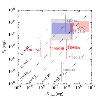
Figure 9.— Fireball kinetic energy $E_{k,\mathrm{iso}}$ at $t=T_{90}$ as estimated from X–ray flux vs. rest–frame isotropic–equivalent gamma–ray energy $E_{\gamma,\mathrm{iso}}$. Red points denote bursts for which $E_{k,\mathrm{iso}}$ can be reliably estimated from the Swift XRT data; gray points denote bursts for which the calculation of $E_{k,\mathrm{iso}}$ may have extreme model dependence. Dashed lines are lines of constant radiative efficiency $\eta=E_{\gamma,\mathrm{iso}}/(E_{k,\mathrm{iso}}+E_{\gamma,\mathrm{iso}})$. The gray, blue, and red rectangles show the 1$\sigma$ parameter ranges of Swift BAT, BAT+GBM, and BAT+LAT long GRBs from Racusin et al. (2011).

5. Looking Forward

In this experiment, we have followed up 35 Fermi GBM bursts, scanning areas from 30 to 147 deg². To date, we have detected eight afterglows with apparent optical magnitudes as bright as $R\approx 16$ and as faint as $R\approx 20$. We have found redshifts as nearby as $z=0.145$ and as distant as $z=3.29$. A continuation of the project should reveal more low–redshift events, more GRB—SNe, and more relatively hard GRBs.

We aim to uncover the much fainter afterglows of short, hard bursts by using stacked P48 exposures and integrating a co-addition stage into the real-time pipeline, and by honing our follow–up to sift through the increased number of candidates. The greatest factor limiting discoveries is, of course, that Fermi detects bursts all over the sky, only a fraction of which are visible from Palomar. Given our success so far, we enthusiastically suggest that other wide–field surveys implement a similar program. Furthermore, automatically sharing lists of candidates between longitudinally separated instruments would facilitate rapid identification and follow–up of the fastest–fading events.

It is uncertain what directions future gamma–ray space missions will take. Some may be like Swift, able to rapidly train multiple on–board follow–up instruments on new targets. Even if they lack these capabilities, we should be able to routinely locate GRB afterglows and find their redshifts using targeted, ground–based optical transient searches similar to the one that we have described.

Looking beyond GRBs, our present effort serves as a prototype for searching for optical counterparts of GW transients. We expect that many of the techniques that we have described and the lessons that we have learned in the context of iPTF will generalize to other wide-field instruments on meter-class and larger telescopes.

Near the end of 2015, Advanced LIGO will begin taking data, with Advanced Virgo soon following suit. The first binary neutron star merger detections are anticipated by 2016 or later (Aasi et al., 2013). On a similar timescale, iPTF will transform into the Zwicky Transient Facility, featuring a new 47 deg² survey camera that can reach $R=20.4$ mag in 30 s. The prime GW sources, binary neutron star (BNS) mergers, may also produce a variety of optical transients: on- or off–axis afterglows (van Eerten & MacFadyen, 2011; Urata et al., 2015), kilonovae (Li & Paczyński, 1998; Barnes & Kasen, 2013), and neutron-powered precursors (Metzger et al., 2015); see Figure 10 for some examples.

There will be two key challenges. First, GW localizations can be even coarser than Fermi GBM error circles. Starting around $\sim$600 deg² in the initial (2015) two–detector configuration (Kasliwal & Nissanke, 2014; Singer et al., 2014e), the areas will shrink to $\sim$200 deg² with the addition of Virgo in 2016. They should reach $\sim 10$ deg² toward the end of the decade as the three detectors approach final design sensitivity and can approach $\sim 1$ deg² as additional planned GW facilities come online (LIGO—India and KAGRA; see Schutz 2011; Veitch et al. 2012; Fairhurst 2014; Nissanke et al. 2013; Aasi et al. 2013). Since the detection efficiency of our GBM–iPTF afterglow search is consistent with the areas that we searched, we expect that even the earliest Advanced LIGO localizations will present no undue difficulties for Zwicky Transient Facility (ZTF) when we consider its 15–fold increase in areal survey rate as compared to iPTF.

However, there is a second challenge that these optical signatures are predicted to be fainter than perhaps $22$ mag (with the exception of on-axis afterglows, which should be rare but bright due to beaming). For meter-size telescopes, this will require integrating for much longer (10 minutes to 1 hr) than we have been performing with iPTF. Fortunately, because the LIGO antenna pattern is preferentially sensitive above and directly opposite of North America, we are optimistic that many early Advanced LIGO events should be promptly accessible from Palomar with long observability windows (Kasliwal & Nissanke, 2014).

The main difficulty for any GW optical counterpart search will be the inundation of false positives due to the required depth and area. We enumerate the following strategies to help identify the one needle in the haystack:

1. Improved machine learning algorithms (see Bue et al. 2014 in the context of iPTF) will decrease the contamination of the discovery stream by artifacts.

2. Combining a catalog of nearby galaxies with the distance and position information from the GW observations can help to reduce and prioritize targets for further follow–up (Nissanke et al., 2013).

3. Better leveraging of light–curve history across multiple surveys will help to automate the selection of targets for photometric follow-up with multiple telescopes.

4. Our first experiences with detections and non-detections will guide decisions about the optimal filter. At the moment, kilonova models prefer redder filters (suggesting $i$ band), and precursor models prefer bluer (suggesting $g$ band).

The combination of gamma-ray missions, ground-based GW detectors, and synoptic optical survey instruments is poised to make major discoveries over the next few years, of which we have provided a small taste in this work. We offer both lessons learned and a way forward in this multimessenger effort. The ultimate reward will be joint observations of a compact binary merger in gamma, X–rays, optical, and GWs, giving us an exceptionally complete record of a complex astrophysical process: it will be almost as good as being there.

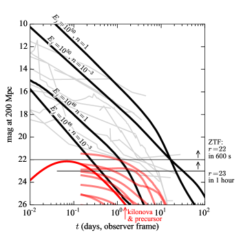
Figure 10.— Light curves of short GRB afterglows, scaled to an Advanced LIGO range of 200 Mpc. Thin gray lines are afterglows of Swift short GRBs that have known redshifts. Thick black lines are synthetic on–axis afterglows from van Eerten & MacFadyen (2011) with jet half–opening angles of 0.2 rad and observer angles of 0 rad. Jet energies $E_{j}$, in units of erg, and circumburst densities $n$, in units of cm^-3, are labeled on the plot. The solid, deep–red line is the $r$–band neutron–powered kilonova precursor model from Metzger et al. (2015) with opacity $\kappa_{r}=30$ cm² g^-1, free neutron mass $m_{n}=10^{-4}$ $M_{\sun}$, and electron fraction $Y_{e}=0.05$. The solid, light–red lines represent kilonova models from Barnes & Kasen (2013) with ejected masses of $m_{\mathrm{ej}}=10^{-3}$, $10^{-2}$, or $10^{-1}~{}M_{\sun}$ and characteristic velocities $\beta=v/c=0.1$, 0.2, or 0.3. The Metzger et al. (2015) kilonova precursors are blue: they peak at about 0.1 mag brighter in the $g$ band than in $r$. The Barnes & Kasen (2013) kilonova models are red: they are about 1 mag brighter in the $i$ band than in $r$.

2MASS

Two Micron All Sky Survey

AdVirgo

Advanced Virgo

AMI

Arcminute Microkelvin Imager

AGN

active galactic nucleus

aLIGO

Advanced LIGO

ATCA

Australia Telescope Compact Array

ATLAS

Asteroid Terrestrial-impact Last Alert System

BAT

Burst Alert Telescope (instrument on Swift)

BATSE

Burst and Transient Source Experiment (instrument on CGRO)

BAYESTAR

BAYESian TriAngulation and Rapid localization

BBH

binary black hole

BHBH

black hole—black hole

BH

black hole

BNS

binary neutron star

CARMA

Combined Array for Research in Millimeter–wave Astronomy

CASA

Common Astronomy Software Applications

CFH12k

Canada–France–Hawaii $12\,288\times 8\,192$ pixel CCD mosaic (instrument formerly on the Canada–France–Hawaii Telescope, now on the P48)

CRTS

Catalina Real-time Transient Survey

CTIO

Cerro Tololo Inter-American Observatory

CBC

compact binary coalescence

CCD

charge coupled device

CDF

cumulative distribution function

CGRO

Compton Gamma Ray Observatory

CMB

cosmic microwave background

CRLB

Cramér—Rao lower bound

cWB

Coherent WaveBurst

DASWG

Data Analysis Software Working Group

DBSP

Double Spectrograph (instrument on P200)

DCT

Discovery Channel Telescope

DECam

Dark Energy Camera (instrument on the Blanco 4–m telescope at CTIO)

DFT

discrete Fourier transform

EM

electromagnetic

FD

frequency domain

FAR

false alarm rate

FFT

fast Fourier transform

FIR

finite impulse response

FITS

Flexible Image Transport System

FLOPS

floating point operations per second

FOV

field of view

FTN

Faulkes Telescope North

GBM

Gamma-ray Burst Monitor (instrument on Fermi)

GCN

Gamma-ray Coordinates Network

GMOS

Gemini Multi-object Spectrograph (instrument on the Gemini telescopes)

GRB

gamma-ray burst

GSL

GNU Scientific Library

GTC

Gran Telescopio Canarias

GW

gravitational wave

HAWC

High–Altitude Water Čerenkov Gamma–Ray Observatory

HCT

Himalayan Chandra Telescope

HEALPix

Hierarchical Equal Area isoLatitude Pixelization

HEASARC

High Energy Astrophysics Science Archive Research Center

HETE

High Energy Transient Explorer

HFOSC

Himalaya Faint Object Spectrograph and Camera (instrument on HCT)

HMXB

high–mass X–ray binary

HSC

Hyper Suprime–Cam (instrument on the 8.2–m Subaru telescope)

IACT

imaging atmospheric Čerenkov telescope

IIR

infinite impulse response

IMACS

Inamori-Magellan Areal Camera & Spectrograph (instrument on the Magellan Baade telescope)

IPAC

Infrared Processing and Analysis Center

IPN

InterPlanetary Network

iPTF

intermediate Palomar Transient Factory

ISM

interstellar medium

KAGRA

KAmioka GRAvitational–wave observatory

KDE

kernel density estimator

LAT

Large Area Telescope

LCOGT

Las Cumbres Observatory Global Telescope

LHO

LIGO Hanford Observatory

LIGO

Laser Interferometer GW Observatory

llGRB

low–luminosity GRB

LLOID

Low Latency Online Inspiral Detection

LLO

LIGO Livingston Observatory

LMI

Large Monolithic Imager (instrument on DCT)

LOFAR

Low Frequency Array

LSB

long, soft burst

LSC

LIGO Scientific Collaboration

LSO

last stable orbit

LSST

Large Synoptic Survey Telescope

LTI

linear time invariant

MAP

maximum a posteriori

MBTA

Multi-Band Template Analysis

MCMC

Markov chain Monte Carlo

MLE

maximum likelihood (ML) estimator

ML

maximum likelihood

NED

NASA/IPAC Extragalactic Database

NSBH

neutron star—black hole

NSBH

neutron star—black hole

NSF

National Science Foundation

NSNS

neutron star—neutron star

NS

neutron star

OT

optical transient

P48

Palomar 48 inch Oschin telescope

P60

robotic Palomar 60 inch telescope

P200

Palomar 200 inch Hale telescope

PC

photon counting

PSD

power spectral density

PSF

point-spread function

PTF

Palomar Transient Factory

QUEST

Quasar Equatorial Survey Team

RAPTOR

Rapid Telescopes for Optical Response

REU

Research Experiences for Undergraduates

RMS

root mean square

ROTSE

Robotic Optical Transient Search

S5

LIGO’s fifth science run

S6

LIGO’s sixth science run

SAA

South Atlantic Anomaly

SHB

short, hard burst

SHGRB

short, hard gamma-ray burst

SMT

Slewing Mirror Telescope (instrument on UFFO Pathfinder)

S/N

signal–to–noise ratio

SSC

synchrotron self–Compton

SDSS

Sloan Digital Sky Survey

SED

spectral energy distribution

SN

supernova

SN Ic–BL

broad–line Type Ic SN

SVD

singular value decomposition

TAROT

Télescopes à Action Rapide pour les Objets Transitoires

TDOA

time delay on arrival

TD

time domain

TOA

time of arrival

TOO

target–of–opportunity

UFFO

Ultra Fast Flash Observatory

UHE

ultra high energy

UVOT

UV/Optical Telescope (instrument on Swift)

VHE

very high energy

VLA

Karl G. Jansky Very Large Array

VLT

Very Large Telescope

WAM

Wide–band All–sky Monitor (instrument on Suzaku)

WCS

World Coordinate System

w.s.s.

wide–sense stationary

XRF

X–ray flash

XRT

X–ray Telescope (instrument on Swift)

ZTF

Zwicky Transient Facility

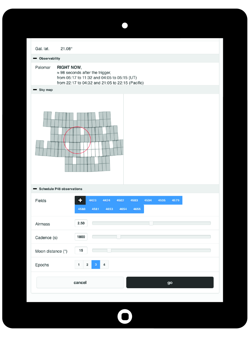
Figure 11.— Screenshot of the iPTF TOO Marshal shortly after a Fermi GBM detection. At this stage, the application presents the recommended P48 fields, the time window of observability, and the history of GCN notices and circulars related to the trigger. It gives the human participants the option to customize the P48 sequence by adding or removing P48 fields and tuning the airmass limit, cadence, or number of images.

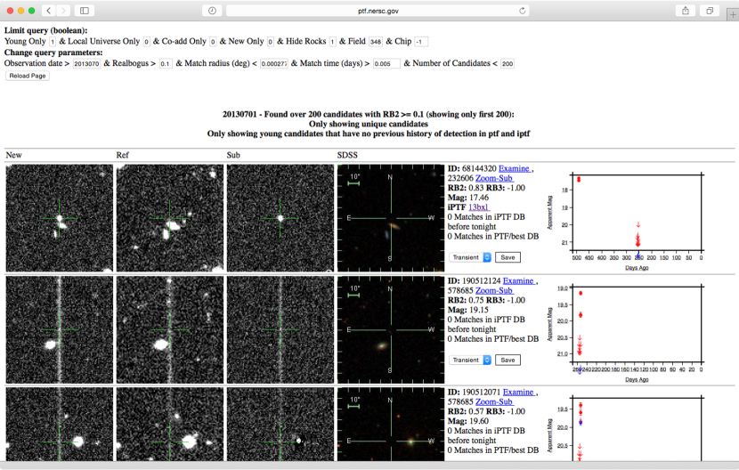
Figure 12.— Screenshot of the Treasures portal, showing new, reference, subtraction, and archival SDSS images as well as P48 light curves. This page is for the date and field containing GRB 130702A / iPTF13bxl.

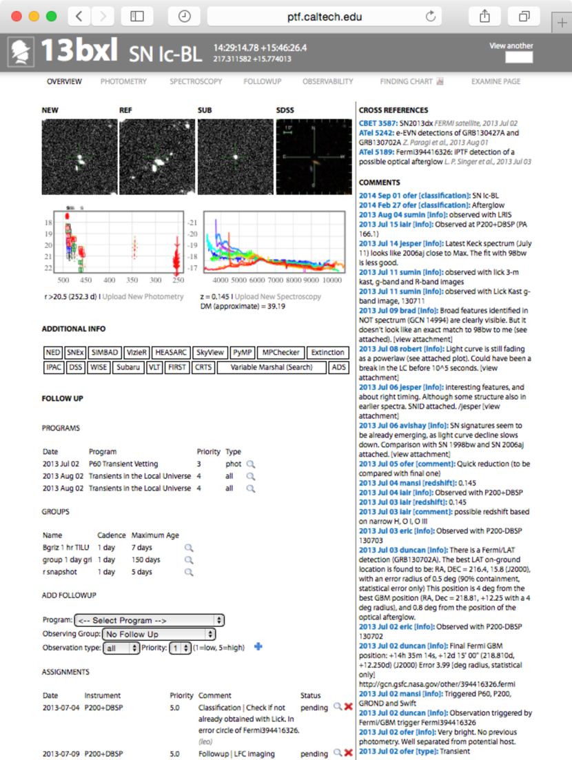
Figure 13.— Screenshot of the iPTF Transient Marshal, showing GRB 130702A / iPTF13bxl.

References

- Aasi et al. (2013) Aasi, J., Abadie, J., Abbott, B. P., et al. 2013, arXiv:1304.0670
- Amaral-Rogers (2014a) Amaral-Rogers, A. 2014a, GCN, 16232, 1
- Amaral-Rogers (2014b) —. 2014b, GCN, 16254, 1
- Amati (2006) Amati, L. 2006, MNRAS, 372, 233
- Amati et al. (2013) Amati, L., Dichiara, S., Frontera, F., et al. 2013, GCN, 15025, 1
- Amati et al. (2009) Amati, L., Frontera, F., & Guidorzi, C. 2009, A&A, 508, 173
- Amati et al. (2008) Amati, L., Guidorzi, C., Frontera, F., et al. 2008, MNRAS, 391, 577
- Amati et al. (2002) Amati, L., Frontera, F., Tavani, M., et al. 2002, A&A, 390, 81
- Anderson et al. (2014a) Anderson, G. E., Staley, T. D., Fender, R. P., Kasliwal, M. M., & Horesh, A. 2014a, GCN, 16725, 1
- Anderson et al. (2014b) Anderson, G. E., van der Horst, A. J., Staley, T. D., et al. 2014b, MNRAS, 440, 2059
- Atteia (2003) Atteia, J.-L. 2003, A&A, 407, L1
- Atwood et al. (2009) Atwood, W. B., Abdo, A. A., Ackermann, M., et al. 2009, ApJ, 697, 1071
- Band & Preece (2005) Band, D. L., & Preece, R. D. 2005, ApJ, 627, 319
- Barnes & Kasen (2013) Barnes, J., & Kasen, D. 2013, ApJ, 775, 18
- Barthelmy et al. (2005) Barthelmy, S. D., Barbier, L. M., Cummings, J. R., et al. 2005, Space Sci. Rev., 120, 143
- Bellm (2014) Bellm, E. C. 2014, arXiv:1410.8185
- Bertin (2006) Bertin, E. 2006, in Astronomical Society of the Pacific Conference Series, Vol. 351, Astronomical Data Analysis Software and Systems XV, ed. C. Gabriel, C. Arviset, D. Ponz, & S. Enrique, 112
- Bertin et al. (2002) Bertin, E., Mellier, Y., Radovich, M., et al. 2002, in Astronomical Society of the Pacific Conference Series, Vol. 281, Astronomical Data Analysis Software and Systems XI, ed. D. A. Bohlender, D. Durand, & T. H. Handley, 228
- Bhalerao & Sahu (2014) Bhalerao, V., & Sahu, D. K. 2014, GCN, 16244, 1
- Bhalerao et al. (2014) Bhalerao, V., Singer, L. P., Kasliwal, M. M., et al. 2014, GCN, 16442, 1
- Bloom et al. (2001) Bloom, J. S., Frail, D. A., & Sari, R. 2001, AJ, 121, 2879
- Bock et al. (2006) Bock, D. C.-J., Bolatto, A. D., Hawkins, D. W., et al. 2006, in SPIE Conf. Series, Vol. 6267, SPIE Conf. Series, 13
- Brink et al. (2013) Brink, H., Richards, J. W., Poznanski, D., et al. 2013, MNRAS, 435, 1047
- Bromberg et al. (2011) Bromberg, O., Nakar, E., & Piran, T. 2011, ApJ, 739, L55
- Bue et al. (2014) Bue, B. D., Wagstaff, K. L., Rebbapragada, U. D., Thompson, D. R., & Tang, B. 2014, in Proceedings of the 2014 conference on Big Data from Space (BiDS’14)
- Bufano et al. (2011) Bufano, F., Benetti, S., Sollerman, J., Pian, E., & Cupani, G. 2011, Astronomische Nachrichten, 332, 262
- Burns (2014) Burns, E. 2014, GCN, 16363, 1
- Burrows et al. (2005) Burrows, D. N., Hill, J. E., Nousek, J. A., et al. 2005, Space Sci. Rev., 120, 165
- Butler et al. (2012) Butler, N., Klein, C., Fox, O., et al. 2012, in SPIE Conf. Series, Vol. 8446, SPIE Conf. Series, 10
- Butler et al. (2013a) Butler, N., Watson, A. M., Kutyrev, A., et al. 2013a, GCN, 14993, 1
- Butler et al. (2013b) —. 2013b, GCN, 14980, 1
- Butler et al. (2014a) —. 2014a, GCN, 16246, 1
- Butler et al. (2014b) —. 2014b, GCN, 16236, 1
- Butler et al. (2010) Butler, N. R., Bloom, J. S., & Poznanski, D. 2010, ApJ, 711, 495
- Butler et al. (2009) Butler, N. R., Kocevski, D., & Bloom, J. S. 2009, ApJ, 694, 76
- Butler et al. (2007) Butler, N. R., Kocevski, D., Bloom, J. S., & Curtis, J. L. 2007, ApJ, 671, 656
- Cabrera et al. (2007) Cabrera, J. I., Firmani, C., Avila-Reese, V., et al. 2007, MNRAS, 382, 342
- Campana et al. (2006) Campana, S., Mangano, V., Blustin, A. J., et al. 2006, Nature, 442, 1008
- Cano et al. (2014) Cano, Z., de Ugarte Postigo, A., Pozanenko, A., et al. 2014, A&A, 568, A19
- Cano et al. (2015) Cano, Z., de Ugarte Postigo, A., Perley, D., et al. 2015, ArXiv e-prints, arXiv:1505.03522
- Cenko et al. (2013a) Cenko, S. B., Gal-Yam, A., Kasliwal, M. M., et al. 2013a, GCN, 14998, 1
- Cenko et al. (2012) Cenko, S. B., Ofek, E. O., & Nugent, P. E. 2012, GCN, 13489, 1
- Cenko et al. (2006) Cenko, S. B., Fox, D. B., Moon, D.-S., et al. 2006, PASP, 118, 1396
- Cenko et al. (2009) Cenko, S. B., Kelemen, J., Harrison, F. A., et al. 2009, ApJ, 693, 1484
- Cenko et al. (2013b) Cenko, S. B., Kulkarni, S. R., Horesh, A., et al. 2013b, ApJ, 769, 130
- Cenko et al. (2014) Cenko, S. B., Kasliwal, M. M., Perley, D. A., et al. 2014, GCN, 15883, 1
- Cepa et al. (2000) Cepa, J., Aguiar, M., Escalera, V. G., et al. 2000, in SPIE Conf. Series, Vol. 4008, Optical and IR Telescope Instrumentation and Detectors, ed. M. Iye & A. F. Moorwood, 623–631
- Chandra & Frail (2012) Chandra, P., & Frail, D. A. 2012, ApJ, 746, 156
- Cheung et al. (2013) Cheung, T., Vianello, G., Zhu, S., et al. 2013, GCN, 14971, 1
- Chevalier & Li (1999) Chevalier, R. A., & Li, Z.-Y. 1999, ApJ, 520, L29
- Chornock et al. (2010) Chornock, R., Berger, E., Levesque, E. M., et al. 2010, arXiv:1004.2262
- Collazzi et al. (2012) Collazzi, A. C., Schaefer, B. E., Goldstein, A., & Preece, R. D. 2012, ApJ, 747, 39
- Connaughton et al. (2015) Connaughton, V., Briggs, M. S., Goldstein, A., et al. 2015, ApJS, 216, 32
- Corder et al. (2010) Corder, S. A., Wright, M. C. H., & Carpenter, J. M. 2010, in SPIE Conf. Series, Vol. 7733, SPIE Conf. Series, 3
- Corsi & Horesh (2014) Corsi, A., & Horesh, A. 2014, GCN, 16694, 1
- Corsi et al. (2012) Corsi, A., Ofek, E. O., Gal-Yam, A., et al. 2012, ApJ, 747, L5
- Cucchiara (2014) Cucchiara, A. 2014, GCN, 15652, 1
- Cutri & et al. (2014) Cutri, R. M., & et al. 2014, VizieR Online Data Catalog, 2328, 0
- Dai & Cheng (2001) Dai, Z. G., & Cheng, K. S. 2001, ApJ, 558, L109
- Dai et al. (2004) Dai, Z. G., Liang, E. W., & Xu, D. 2004, ApJ, 612, L101
- D’Avanzo et al. (2013) D’Avanzo, P., Porterfield, B., Burrows, D. N., et al. 2013, GCN, 14973, 1
- De Pasquale (2014a) De Pasquale, M. 2014a, GCN, 16455, 1
- De Pasquale (2014b) —. 2014b, GCN, 16428, 1
- D’Elia & Izzo (2014) D’Elia, V., & Izzo, L. 2014, GCN, 16464, 1
- D’Elia et al. (2014) D’Elia, V., Marshall, F. E., & Malesani, D. 2014, GCN, 16451, 1
- D’Elia et al. (2013) D’Elia, V., D’Avanzo, P., Melandri, A., et al. 2013, GCN, 15000, 1
- Drake et al. (2009) Drake, A. J., Djorgovski, S. G., Mahabal, A., et al. 2009, ApJ, 696, 870
- Evans et al. (2007) Evans, P. A., Beardmore, A. P., Page, K. L., et al. 2007, A&A, 469, 379
- Evans et al. (2009) —. 2009, MNRAS, 397, 1177
- Fairhurst (2014) Fairhurst, S. 2014, Journal of Physics Conference Series, 484, 012007
- Firmani et al. (2009) Firmani, C., Cabrera, J. I., Avila-Reese, V., et al. 2009, MNRAS, 393, 1209
- Fitzpatrick & Connaughton (2014) Fitzpatrick, G., & Connaughton, V. 2014, GCN, 16426, 1
- Flesch (2010) Flesch, E. 2010, PASA, 27, 283
- Frater et al. (1992) Frater, R. H., Brooks, J. W., & Whiteoak, J. B. 1992, Journal of Electrical and Electronics Engineering Australia, 12, 103
- Freedman & Waxman (2001) Freedman, D. L., & Waxman, E. 2001, ApJ, 547, 922
- Friedman & Bloom (2005) Friedman, A. S., & Bloom, J. S. 2005, ApJ, 627, 1
- Fujiwara et al. (2014) Fujiwara, T., Yoshii, T., Saito, Y., et al. 2014, GCN, 16259, 1
- Gal-Yam et al. (2011) Gal-Yam, A., Kasliwal, M. M., Arcavi, I., et al. 2011, ApJ, 736, 159
- Gal-Yam et al. (2014) Gal-Yam, A., Arcavi, I., Ofek, E. O., et al. 2014, Nature, 509, 471
- Galama et al. (1998) Galama, T. J., Vreeswijk, P. M., van Paradijs, J., et al. 1998, Nature, 395, 670
- Gehrels et al. (2004) Gehrels, N., Chincarini, G., Giommi, P., et al. 2004, ApJ, 611, 1005
- Ghirlanda et al. (2005) Ghirlanda, G., Ghisellini, G., & Firmani, C. 2005, MNRAS, 361, L10
- Ghirlanda et al. (2006) —. 2006, New Journal of Physics, 8, 123
- Goad et al. (2007) Goad, M. R., Tyler, L. G., Beardmore, A. P., et al. 2007, A&A, 476, 1401
- Goldstein et al. (2012) Goldstein, A., Burgess, J. M., Preece, R. D., et al. 2012, ApJS, 199, 19
- Gorosabel et al. (2014a) Gorosabel, J., de Ugarte Postigo, A., Thoene, C., Perley, D., & Rodriguez, A. G. 2014a, GCN, 16671, 1
- Gorosabel et al. (2014b) Gorosabel, J., Sanchez-Lavega, A., Perez-Hoyos, S., et al. 2014b, GCN, 16227, 1
- Górski et al. (2005) Górski, K. M., Hivon, E., Banday, A. J., et al. 2005, ApJ, 622, 759
- Greiner et al. (2008) Greiner, J., Bornemann, W., Clemens, C., et al. 2008, PASP, 120, 405
- Hancock et al. (2013) Hancock, P., Murphy, T., Gaensler, B., Bell, M., & Burlon, D. 2013, GCN, 15395, 1
- Heussaff et al. (2013) Heussaff, V., Atteia, J.-L., & Zolnierowski, Y. 2013, A&A, 557, A100
- Hjorth & Bloom (2012) Hjorth, J., & Bloom, J. S. 2012, The Gamma-Ray Burst - Supernova Connection, 169–190
- Holland & Mangano (2014) Holland, S. T., & Mangano, V. 2014, GCN, 15673, 1
- Hook et al. (2004) Hook, I. M., Jørgensen, I., Allington-Smith, J. R., et al. 2004, PASP, 116, 425
- Horesh et al. (2014) Horesh, A., Singer, L. P., Cenko, S. B., Kasliwal, M. M., & Perley, D. 2014, GCN, 16266, 1
- Howell et al. (2005) Howell, D. A., Sullivan, M., Perrett, K., et al. 2005, ApJ, 634, 1190
- Hurley et al. (2013) Hurley, K., Goldsten, J., Connaughton, V., et al. 2013, GCN, 14974, 1
- Hurley et al. (2014a) Hurley, K., Goldsten, J., Mitrofanov, I. G., et al. 2014a, GCN, 15864, 1
- Hurley et al. (2014b) Hurley, K., Golenetskii, S., Aptekar, R., et al. 2014b, GCN, 15888, 1
- Hurley et al. (2014c) Hurley, K., Goldsten, J., Golenetskii, S., et al. 2014c, GCN, 16225, 1
- Hurley et al. (2014d) —. 2014d, GCN, 16369, 1
- Jenke (2013) Jenke, P. 2013, GCN, 15331, 1
- Jenke & Xiong (2014) Jenke, P., & Xiong, S. 2014, GCN, 15644, 1
- Kaiser et al. (2010) Kaiser, N., Burgett, W., Chambers, K., et al. 2010, in SPIE Conf. Series, Vol. 7733, SPIE Conf. Series, 0
- Kann et al. (2010) Kann, D. A., Klose, S., Zhang, B., et al. 2010, ApJ, 720, 1513
- Kann et al. (2011) —. 2011, ApJ, 734, 96
- Kasliwal (2011) Kasliwal, M. M. 2011, PhD thesis, California Institute of Technology
- Kasliwal et al. (2014) Kasliwal, M. M., Cenko, S. B., & Singer, L. P. 2014, GCN, 16425, 1
- Kasliwal & Nissanke (2014) Kasliwal, M. M., & Nissanke, S. 2014, ApJ, 789, L5
- Kasliwal et al. (2013) Kasliwal, M. M., Singer, L. P., & Cenko, S. B. 2013, GCN, 15324, 1
- Kasliwal et al. (2012) Kasliwal, M. M., Kulkarni, S. R., Gal-Yam, A., et al. 2012, ApJ, 755, 161
- Kelemen (2014) Kelemen, J. 2014, GCN, 16440, 1
- Kelly et al. (2013) Kelly, P. L., Filippenko, A. V., Fox, O. D., Zheng, W., & Clubb, K. I. 2013, ApJ, 775, L5
- Klose et al. (2013) Klose, S., Nicuesa Guelbenzu, A., Kruehler, T., et al. 2013, GCN, 15320, 1
- Kocevski (2012) Kocevski, D. 2012, ApJ, 747, 146
- Krimm et al. (2009) Krimm, H. A., Yamaoka, K., Sugita, S., et al. 2009, ApJ, 704, 1405
- Kulkarni (2012) Kulkarni, S. R. 2012, in IAU Symposium, Vol. 285, IAU Symposium, ed. E. Griffin, R. Hanisch, & R. Seaman, 55–61
- Kulkarni et al. (1998) Kulkarni, S. R., Frail, D. A., Wieringa, M. H., et al. 1998, Nature, 395, 663
- Laskar et al. (2013) Laskar, T., Berger, E., Zauderer, B. A., et al. 2013, ApJ, 776, 119
- Law et al. (2009) Law, N. M., Kulkarni, S. R., Dekany, R. G., et al. 2009, PASP, 121, 1395
- Leloudas et al. (2013) Leloudas, G., Fynbo, J. P. U., Schulze, S., et al. 2013, GCN, 14983, 1
- Li & Paczyński (1998) Li, L.-X., & Paczyński, B. 1998, ApJ, 507, L59
- Li et al. (2011) Li, W., Leaman, J., Chornock, R., et al. 2011, MNRAS, 412, 1441
- Li & Hjorth (2014) Li, X., & Hjorth, J. 2014, arXiv:1407.3506
- Lloyd-Ronning & Zhang (2004) Lloyd-Ronning, N. M., & Zhang, B. 2004, ApJ, 613, 477
- Malesani et al. (2014) Malesani, D., Xu, D., D’Avanzo, P., Palazzi, E., & Perna, D. 2014, GCN, 16229, 1
- Malesani et al. (2013) Malesani, D., Xu, D., Losada, I. R., & Duval, F. 2013, GCN, 15642, 1
- Mangano (2014) Mangano, V. 2014, GCN, 16412, 1
- Mangano & Burrows (2014) Mangano, V., & Burrows, D. N. 2014, GCN, 16373, 1
- Mangano et al. (2014a) Mangano, V., Evans, P. A., & Goad, M. R. 2014a, GCN, 16366, 1
- Mangano et al. (2014b) Mangano, V., Page, K., & Malesani, D. 2014b, GCN, 15648, 1
- Marshall & Amarel-Rogers (2014) Marshall, F. E., & Amarel-Rogers, A. 2014, GCN, 16243, 1
- Masi (2014) Masi, G. 2014, GCN, 16235, 1
- Meegan et al. (2009) Meegan, C., Lichti, G., Bhat, P. N., et al. 2009, ApJ, 702, 791
- Melandri et al. (2012) Melandri, A., Pian, E., Ferrero, P., et al. 2012, A&A, 547, A82
- Metzger et al. (2015) Metzger, B. D., Bauswein, A., Goriely, S., & Kasen, D. 2015, MNRAS, 446, 1115
- Modjaz et al. (2006) Modjaz, M., Stanek, K. Z., Garnavich, P. M., et al. 2006, ApJ, 645, L21
- Moskvitin et al. (2014) Moskvitin, A. S., Makarov, D. I., Valeev, A. F., et al. 2014, GCN, 16228, 1
- Mulchaey et al. (2013) Mulchaey, J., Kasliwal, M. M., Arcavi, I., Bellm, E., & Kelson, D. 2013, GCN, 14985, 1
- Nakar & Piran (2005) Nakar, E., & Piran, T. 2005, MNRAS, 360, L73
- Nakar & Sari (2012) Nakar, E., & Sari, R. 2012, ApJ, 747, 88
- Nissanke et al. (2013) Nissanke, S., Kasliwal, M., & Georgieva, A. 2013, ApJ, 767, 124
- Nugent et al. (2011) Nugent, P. E., Sullivan, M., Cenko, S. B., et al. 2011, Nature, 480, 344
- Nysewander et al. (2009) Nysewander, M., Fruchter, A. S., & Pe’er, A. 2009, ApJ, 701, 824
- Oates & Cenko (2014) Oates, S. R., & Cenko, S. B. 2014, GCN, 16672, 1
- Ochsenbein et al. (2000) Ochsenbein, F., Bauer, P., & Marcout, J. 2000, A&AS, 143, 23
- Ofek et al. (2012) Ofek, E. O., Laher, R., Law, N., et al. 2012, PASP, 124, 62
- Ofek et al. (2013) Ofek, E. O., Sullivan, M., Cenko, S. B., et al. 2013, Nature, 494, 65
- Oke & Gunn (1983) Oke, J. B., & Gunn, J. E. 1983, ApJ, 266, 713
- Paciesas et al. (2012a) Paciesas, W. S., Meegan, C. A., von Kienlin, A., et al. 2012a, ApJS, 199, 18
- Paciesas et al. (2012b) —. 2012b, ApJS, 199, 18
- Page (2013) Page, K. L. 2013, GCN, 15329, 1
- Page & Cenko (2014) Page, K. L., & Cenko, S. B. 2014, GCN, 16682, 1
- Page et al. (2014) Page, K. L., Evans, P. A., & Cenko, S. B. 2014, GCN, 16670, 1
- Panaitescu (2005) Panaitescu, A. 2005, MNRAS, 362, 921
- Perley (2014) Perley, D. A. 2014, GCN, 15680, 1
- Perley et al. (2014a) Perley, D. A., Cao, Y., Kasliwal, M., & Kirby, E. 2014a, GCN, 16365, 1
- Perley et al. (2013) Perley, D. A., Cenko, S. B., & Kasliwal, M. M. 2013, GCN, 15327, 1
- Perley et al. (2014b) Perley, D. A., Graham, M. L., Filippenko, A. V., & Cenko, S. B. 2014b, GCN, 16454, 1
- Perley et al. (2014c) Perley, D. A., Kasliwal, M., Singer, L. P., Cao, Y., & Tinyanont, K. 2014c, GCN, 16387, 1
- Perley & Singer (2014) Perley, D. A., & Singer, L. 2014, GCN, 16362, 1
- Perley et al. (2014d) Perley, D. A., Cenko, S. B., Corsi, A., et al. 2014d, ApJ, 781, 37
- Pescalli et al. (2015) Pescalli, A., Ghirlanda, G., Salafia, O. S., et al. 2015, MNRAS, 447, 1911
- Phillips (1993) Phillips, M. M. 1993, ApJ, 413, L105
- Pian et al. (2006) Pian, E., Mazzali, P. A., Masetti, N., et al. 2006, Nature, 442, 1011
- Pozanenko et al. (2013) Pozanenko, A., Volnova, A., Burhonov, O., & Molotov, I. 2013, GCN, 14996, 1
- Quimby et al. (2011) Quimby, R. M., Kulkarni, S. R., Kasliwal, M. M., et al. 2011, Nature, 474, 487
- Racusin et al. (2011) Racusin, J. L., Oates, S. R., Schady, P., et al. 2011, ApJ, 738, 138
- Rahmer et al. (2008) Rahmer, G., Smith, R., Velur, V., et al. 2008, in SPIE Conf. Series, Vol. 7014, SPIE Conf. Series, 4
- Rau et al. (2013) Rau, A., Kruehler, T., & Greiner, J. 2013, GCN, 15330, 1
- Rau et al. (2009) Rau, A., Kulkarni, S. R., Law, N. M., et al. 2009, PASP, 121, 1334
- Rees & Meszaros (1994) Rees, M. J., & Meszaros, P. 1994, ApJ, 430, L93
- Richardson et al. (2002) Richardson, D., Branch, D., Casebeer, D., et al. 2002, AJ, 123, 745
- Robitaille et al. (2013) Robitaille, T. P., Tollerud, E. J., Greenfield, P., et al. 2013, A&A, 558, A33
- Roming et al. (2005) Roming, P. W. A., Kennedy, T. E., Mason, K. O., et al. 2005, Space Sci. Rev., 120, 95
- Sahu et al. (2014) Sahu, D. K., Bhalerao, V., & Anupama, G. C. 2014, GCN, 16684, 1
- Sakamoto et al. (2006) Sakamoto, T., Barbier, L., Barthelmy, S. D., et al. 2006, ApJ, 636, L73
- Sari et al. (1998) Sari, R., Piran, T., & Narayan, R. 1998, ApJ, 497, L17
- Schaefer & Collazzi (2007) Schaefer, B. E., & Collazzi, A. C. 2007, ApJ, 656, L53
- Schulze et al. (2013) Schulze, S., Leloudas, G., Xu, D., et al. 2013, GCN, 14994, 1
- Schulze et al. (2014a) Schulze, S., Malesani, D., Cucchiara, A., et al. 2014a, A&A, 566, A102
- Schulze et al. (2014b) —. 2014b, A&A, 566, A102
- Schutz (2011) Schutz, B. F. 2011, Class. Quantum Grav., 28, 125023
- Shahmoradi & Nemiroff (2011) Shahmoradi, A., & Nemiroff, R. J. 2011, MNRAS, 411, 1843
- Siegel & De Pasquale (2014) Siegel, M. H., & De Pasquale, M. 2014, GCN, 16432, 1
- Singer et al. (2013a) Singer, L. P., Cenko, S. B., & Kasliwal, M. M. 2013a, GCN, 15643, 1
- Singer et al. (2014a) Singer, L. P., Cenko, S. B., Kasliwal, M. M., Fremling, C., & Dzigan, Y. 2014a, GCN, 16226, 1
- Singer et al. (2014b) Singer, L. P., Kasliwal, M. M., Bhalerao, V. B., et al. 2014b, GCN, 16668, 1
- Singer et al. (2014c) Singer, L. P., Kasliwal, M. M., & Cenko, S. B. 2014c, GCN, 16360, 1
- Singer et al. (2014d) —. 2014d, GCN, 15878, 1
- Singer et al. (2013b) Singer, L. P., Cenko, S. B., Kasliwal, M. M., et al. 2013b, ApJ, 776, L34
- Singer et al. (2013c) —. 2013c, GCN, 14967, 1
- Singer et al. (2014e) Singer, L. P., Price, L. R., Farr, B., et al. 2014e, ApJ, 795, 105
- Skrutskie et al. (2006) Skrutskie, M. F., Cutri, R. M., Stiening, R., et al. 2006, AJ, 131, 1163
- Smith et al. (2014) Smith, R. M., Dekany, R. G., Bebek, C., et al. 2014, in SPIE Conf. Series, Vol. 9147, SPIE Conf. Series, 79
- Sollerman et al. (2006) Sollerman, J., Jaunsen, A. O., Fynbo, J. P. U., et al. 2006, A&A, 454, 503
- Sonbas et al. (2013) Sonbas, E., Racusin, J. L., Kocevski, D., & McEnery, J. 2013, GCN, 15640, 1
- Sudilovsky et al. (2013) Sudilovsky, V., Tanga, M., & Greiner, J. 2013, GCN, 15328, 1
- Svensson et al. (2010) Svensson, K. M., Levan, A. J., Tanvir, N. R., Fruchter, A. S., & Strolger, L.-G. 2010, MNRAS, 405, 57
- Svirski & Nakar (2014a) Svirski, G., & Nakar, E. 2014a, ApJ, 788, L14
- Svirski & Nakar (2014b) —. 2014b, ApJ, 788, 113
- Urata et al. (2012) Urata, Y., Huang, K., Yamaoka, K., Tsai, P. P., & Tashiro, M. S. 2012, ApJ, 748, L4
- Urata et al. (2015) Urata, Y., Huang, K., Yamazaki, R., & Sakamoto, T. 2015, ApJ, in press, arXiv:1504.07288
- Urata et al. (2014) Urata, Y., Huang, K., Takahashi, S., et al. 2014, ApJ, 789, 146
- van Eerten & MacFadyen (2011) van Eerten, H. J., & MacFadyen, A. I. 2011, ApJ, 733, L37
- Veitch et al. (2012) Veitch, J., Mandel, I., Aylott, B., et al. 2012, Phys. Rev. D, 85, 104045
- Véron-Cetty & Véron (2010) Véron-Cetty, M.-P., & Véron, P. 2010, A&A, 518, A10
- Volnova et al. (2013) Volnova, A., Inasaridze, R., Inasaridze, G., et al. 2013, GCN, 15341, 1
- Volnova et al. (2014a) Volnova, A., Klunko, E., Eselevich, M., Korobtsev, I., & Pozanenko, A. 2014a, GCN, 16260, 1
- Volnova et al. (2014b) Volnova, A., Mundrzyjewski, W., Kusakin, A., & Pozanenko, A. 2014b, GCN, 16453, 1
- von Kienlin (2014) von Kienlin, A. 2014, GCN, 16450, 1
- Wiersema et al. (2014) Wiersema, K., Tanvir, N., Levan, A., & Karjalainen, R. 2014, GCN, 16231, 1
- Wright et al. (2010) Wright, E. L., Eisenhardt, P. R. M., Mainzer, A. K., et al. 2010, AJ, 140, 1868
- Xu et al. (2013a) Xu, D., Malesani, D., Kruehler, T., et al. 2013a, GCN, 15325, 1
- Xu et al. (2013b) Xu, D., Niu, H.-B., Zhang, X., & Esamdin, A. 2013b, GCN, 15641, 1
- Xu et al. (2013c) Xu, D., Zhang, C.-M., & Cao, C. 2013c, GCN, 15326, 1
- Xu et al. (2013d) Xu, D., de Ugarte Postigo, A., Leloudas, G., et al. 2013d, ApJ, 776, 98
- Yu & Goldstein (2014) Yu, H.-F., & Goldstein, A. 2014, GCN, 16224, 1
- Zhang (2014) Zhang, B. 2014, GCN, 16669, 1
- Zwart et al. (2008) Zwart, J. T. L., Barker, R. W., Biddulph, P., et al. 2008, MNRAS, 391, 1545