Nucleation of a three-state spin model on complex networks

Abstract

We study the metastability and nucleation of the Blume-Capel model on complex networks, in which each node can take one of three possible spin variables $\left\{{-1,0,1}\right\}$. We consider the external magnetic field $h$ to be positive, and let the chemical potential $\lambda$ vary between $-h$ and $h$ in a low temperature, such that the $1$ configuration is stable, and $-1$ configuration and/or $0$ configuration are metastable. Combining the heterogeneous mean-field theory with simulations, we show that there exist four regions with distinct nucleation scenarios depending on the values of $h$ and $\lambda$: the system undergoes a two-step nucleation process from $-1$ configuration to $0$ configuration and then to $1$ configuration (region I); nucleation becomes a one-step process without an intermediate metastable configuration directly from $-1$ configuration to $1$ configuration (region II(1)) or directly from $0$ configuration to $1$ configuration (region II(2)) depending on the sign of $\lambda$; the metastability of the system vanishes and nucleation is thus irrelevant (region III). Furthermore, we show that in the region I nucleation rates for each step intersect that results in the occurrence of a maximum in the total nucleation rate.

I Introduction

Complex networks describe not only the pattern discovered ubiquitously in the real world, but also provide a unified theoretical framework to understand the inherent complexity in nature Watts and Strogatz (1998); Barabási and Albert (1999). A central topic in this field is to unveil the relationship between the topology of a network and dynamics taking place on it Albert and Barabási (2002); Newman (2003); Boccaletti et al. (2006); Arenas et al. (2008). In particular, phase transitions on complex networks have been a subject of intense research in the field of statistical physics and many other disciplines Dorogovtsev et al. (2008). Extensive research interests have focused on the onset of phase transitions in diverse network topologies. Owing to the heterogeneity in degree distribution, phase transitions on complex networks are drastically different from those on regular lattices in Euclidean space. For instance, degree heterogeneity can lead to a vanishing percolation threshold Cohen et al. (2000), the whole infection of disease with any small spreading rate Pastor-Satorras and Vespignani (2001), the Ising model to be ordered at all temperatures Aleksiejuk et al. (2002); Bianconi (2002); Dorogovtsev et al. (2002), the disorder-order transition in voter models Lambiotte (2007), synchronization to be suppressed Nishikawa et al. (2003); Motter et al. (2005) and different paths towards synchronization in oscillator network Gómez-Gardeñes et al. (2007), spontaneous differentiation of nonequilibrium pattern Nakao and Mikhailov (2010), to list just a few. However, there is much less attention paid to the dynamics of a phase transition itself on complex networks, such as nucleation in a first-order phase transition.

Nucleation is a fluctuation-driven process that initiates the decay of a metastable state into a more stable one Kashchiev (2000). Many important phenomena in nature, like crystallization Auer and Frenkel (2001), glass formation Johnson et al. (1998), and protein folding Fersht (1995), are closely related to the nucleation process. In the context of complex networks, the study of the nucleation process is not only of theoretical importance for understanding how a first-order phase transition happens in networked systems, but also may have potential implications for controlling fluctuation-driven system-wide transitions in real situations, such as the transitions between different dynamical attractors in neural networks Bar-Yam and Epstein (2004), the genetic switch between high- and low-expression states in gene regulatory networks Tian and Burrage (2006); Koseska et al. (2009), a new opinion Lambiotte and Ausloos (2007) or scientific paradigm formation Bornholdt et al. (2011) as well as language replacement Ke et al. (2008); Wichmann et al. (2008) in social networks, and spontaneous traffic jamming Echenique et al. (2005), synchronization Gómez-Gardeñes et al. (2011); Leyva et al. (2012), cascading failure Buldyrev et al. (2010) and recovery Majdandzic et al. (2014) close to an explosive phase transition.

Recently, we have made a tentative step in the study of the nucleation process of the two-state Ising model on complex networks, where we have identified nucleation pathways, such as nucleating from nodes with smaller degree on heterogeneous networks Chen et al. (2011) and a multi-step nucleation process on modular networks Chen and Hou (2011). In addition, a size-effect of the nucleation rate on mean-field-type networks Chen et al. (2011) and a nonmonotonic dependences of the nucleation rate on the modularity of networks Chen and Hou (2011) and on the degree heterogeneity Chen et al. (2013) were reported. However, many real systems possess complicated free-energy landscape with several local minima where phase transition happens usually via these intermediate metastable states Wales (2003). The presence of intermediate metastable states has been shown to play a key role in determining the pathway and rate of nucleation. For example, it was recently reported that an intermediate metastable phase can provide an easier pathway for the growth of crystal nuclei from fluids, with implications for the crystallization of protein and colloid ten Wolde and Frenkel (1997); Lutsko and Nicolis (2006); Schilling et al. (2010); Tóth et al. (2011); Tan et al. (2014). Thus, it is natural to generalize the nucleation of the two-state Ising model to a three-state spin model on complex networks in which an intermediate metastable state may exist.

In this paper, we shall use the three-state Blume-Capel (BC) model to investigate the nucleation on complex networks. The BC model is a spin-1 Ising model that has been introduced, by Blume Blume (1966) and Capel Capel (1966) independently, as a model for magnetic systems and then applied to multicomponent fluids Mukamel and Blume (1974). The BC model defined on a two-dimensional lattice has been previously used to study the metastability and nucleation in the limit of zero temperature Cirillo and Oliveri (1996) and in the absence of external magnetic field Ekiz et al. (2001). Recently, a reentrance phase transition has been observed in the BC model defined on heterogeneous networks Martino et al. (2012). Here, we show, by using mean-field analysis and simulation, that there are four distinct regions corresponding to different nucleation scenarios for the networked BC model. Depending on the model’s parameters, the system undergoes either a two-step nucleation process with an intermediate metastable state or a one-step nucleation process. We also calculate the rates of nucleation by a rare-event sampling method that agree with the theoretical predictions by evaluating the free-energy barrier to nucleate.

II Model

We consider the BC model defined on a network, where spin variable of each node can take three possible values ${\sigma_{i}}\in\{-1,0,1\}$, and interacting according to the Hamiltonian

$$\mathcal{H}=J\sum\limits_{i<j}{{a_{ij}}{{\left({{\sigma_{i}}-{\sigma_{j}}}\right)}^{2}}-\lambda\sum\limits_{i}{\sigma_{i}^{2}-h\sum\limits_{i}{{\sigma_{i}}}}},$$ (1)

where $J$ is the ferromagnetic interaction constant among nodes, $\lambda$ and $h$ have the meaning of the chemical potential and the external magnetic field imposed on each node, respectively. The elements of the adjacency matrix of the network take $a_{ij}=1$ if nodes $i$ and $j$ are connected and $a_{ij}=0$ otherwise.

The present paper is devoted to the study of metastability and nucleation of the networked three-state BC model at the low temperature. For the purpose, we first consider the stability of the system in the zero temperature limit. In this case, the (local) stable equilibrium refer to the configurations with all the spins equal to $-1$, $0$, $1$, respectively. For the sake of convenience, we use $\uline{-1}$, $\uline{0}$, $\uline{1}$ to denote these stable ordered configurations, respectively. Their energy are as follows: $h-\lambda$, $0$, and $-h-\lambda$. Since we want to study the nucleation from $\uline{-1}$ to $\uline{0}$, and then to $\uline{1}$, we set $\uline{-1}<\uline{0}<\uline{1}$ as the relative stabilities of these configurations. To the end, it is required that $h-\lambda>0>-h-\lambda$, or equivalently, $-h<\lambda<h$ and $h>0$. Due to the small thermal fluctuation at the low temperature, it is expected that the behavior at the low temperature is similar to that at the zero temperature. However, in the presence of small thermal fluctuation the notations $\uline{-1}$, $\uline{0}$, $\uline{1}$ refer to the configurations with most instead of all the spins equal to $-1$, $0$, $1$, respectively. Here, the temperature is fixed at $T=5$ (in unit of $J/k_{B}$) throughout the paper where $k_{B}$ is the Boltzmann constant.

III Theory and Simulation

To proceed the heterogeneous mean-field theory, we first define $X_{k}^{\left(\alpha\right)}$ as the probability that a node of degree $k$ is in the state $\alpha\in\{-1,0,1\}$. The interaction energy of an edge connecting a $k$-degree node and a $k^{\prime}$-degree node is thus written as,

$${E_{kk^{\prime}}} = J\left[{X_{k}^{\left(1\right)}\left({X_{k^{\prime}}^{\left(0\right)}+4X_{k^{\prime}}^{\left({-1}\right)}}\right)+X_{k}^{\left(0\right)}\left({X_{k^{\prime}}^{\left(1\right)}+X_{k^{\prime}}^{\left({-1}\right)}}\right)+X_{k}^{\left({-1}\right)}\left({X_{k^{\prime}}^{\left(0\right)}+4X_{k^{\prime}}^{\left(1\right)}}\right)}\right]$$ (2)

$$= J\left({{Q_{k}}+{Q_{k^{\prime}}}-2{M_{k}}{M_{k^{\prime}}}}\right),$$

where

$$M_{k}=X_{k}^{\left(1\right)}-X_{k}^{\left({-1}\right)}$$ (3a)

$$Q_{k}=X_{k}^{\left(1\right)}+X_{k}^{\left({-1}\right)}$$ (3b)

are the average magnetization and the average squared magnetization of a node of degree $k$, respectively.

Plus the single-node energy, the total energy of the system can be expressed as

$$E = \frac{1}{2}N\sum\limits_{k}{P(k)k\sum\limits_{k^{\prime}}{P(k^{\prime}|k)}}{E_{kk^{\prime}}}-\lambda N\sum\limits_{k}{P(k)}{Q_{k}}-hN\sum\limits_{k}{P(k)}{M_{k}}$$ (4)

$$= JN\left\langle k\right\rangle\left({Q^{\prime}-{{M^{\prime}}^{2}}}\right)-\lambda NQ-hNM$$

where $P(k)$ is the degree distribution, and ${P(k^{\prime}|k)}$ is the conditional probability that a node of degree $k$ links to a node of degree $k^{\prime}$. We use $P(k^{\prime}|k)={{k^{\prime}P(k^{\prime})}\mathord{\left/{\vphantom{{k^{\prime}P(k^{\prime})}{\left\langle k\right\rangle}}}\right.\kern-1.2pt}{\left\langle k\right\rangle}}$ under the consideration of without degree correlation, where ${\left\langle k\right\rangle}$ is the average degree. In Eq.(4), we have used the definitions,

$$M =\sum\limits_{k}{P(k){M_{k}}}$$ (5a)

$$Q =\sum\limits_{k}{P(k){Q_{k}}}$$ (5b)

$$M^{\prime} =\sum\limits_{k}{\frac{{kP(k)}}{{\left\langle k\right\rangle}}{M_{k}}}$$ (5c)

$$Q^{\prime} =\sum\limits_{k}{\frac{{kP(k)}}{{\left\langle k\right\rangle}}{Q_{k}}}$$ (5d)

where $M$ and $Q$ are the average magnetization and the average squared magnetization per node, respectively. $M^{\prime}$ and $Q^{\prime}$ are the average magnetization and the average squared magnetization of a randomly chosen nearest node, respectively.

Furthermore, let us define $S_{k}$ as the entropy of a node of degree $k$, the total entropy of the system is

$$S=N\sum\limits_{k}{P(k)}{S_{k}},$$ (6)

with

$${S_{k}}=-{k_{B}}\sum\limits_{\alpha}{X_{k}^{\left(\alpha\right)}\ln X_{k}^{\left(\alpha\right)}}.$$ (7)

Combining Eqs.(4) and (6), we can get the expression of free energy, $F=E-TS$.

In order to get the extrema of the free energy, we use the Lagrange function,

$$\phi=-f+\sum\limits_{k}{P(k){\mu_{k}}}\left({1-\sum\limits_{\alpha}{X_{k}^{(\alpha)}}}\right),$$ (8)

where $f=F/N$ is the average free energy per node, and $\mu_{k}$ is the Lagrange multiplier to maintain the normalization condition. By minimizing of Eq.(8) with respect to $X_{k}^{(\alpha)}$, one has,

$$X_{k}^{(\alpha)}=\frac{{\exp\left[{-\beta\left({\frac{{\partial e}}{{\partial X_{k}^{(\alpha)}}}}\right)}\right]}}{{\sum\limits_{\alpha}{\exp\left[{-\beta\left({\frac{{\partial e}}{{\partial X_{k}^{(\alpha)}}}}\right)}\right]}}},$$ (9)

with

$$\left\{\begin{array}[]{l}\frac{{\partial e}}{{\partial X_{k}^{(1)}}}=Jk\left({1-2M^{\prime}}\right)-\lambda-h\\ \frac{{\partial e}}{{\partial X_{k}^{(0)}}}=0\\ \frac{{\partial e}}{{\partial X_{k}^{(-1)}}}=Jk\left({1+2M^{\prime}}\right)-\lambda+h\end{array}\right.$$ (13)

where $\beta=1/(k_{B}T)$ and $e=E/N$ is the average energy per node.

Substituting Eq.(9) into Eq.(3), we get

$${M_{k}}=\frac{{2\sinh\left[{\beta\left({2JkM^{\prime}+h}\right)}\right]}}{{2\cosh\left[{\beta\left({2JkM^{\prime}+h}\right)}\right]+\exp\left[{\beta\left({Jk-\lambda}\right)}\right]}}$$ (14)

$${Q_{k}}=\frac{{2\cosh\left[{\beta\left({2JkM^{\prime}+h}\right)}\right]}}{{2\cosh\left[{\beta\left({2JkM^{\prime}+h}\right)}\right]+\exp\left[{\beta\left({Jk-\lambda}\right)}\right]}}$$ (15)

Furthermore, inserting Eq.(11) into Eq.(5c), we get a self-consistent equation of $M^{\prime}$ that can be numerically solved,

$$M^{\prime}=\sum\limits_{k}{\frac{{kP(k)}}{{\left\langle k\right\rangle}}}\frac{{2\sinh\left[{\beta\left({2JkM^{\prime}+h}\right)}\right]}}{{2\cosh\left[{\beta\left({2JkM^{\prime}+h}\right)}\right]+\exp\left[{\beta\left({Jk-\lambda}\right)}\right]}}$$ (16)

Once the solutions of $M^{\prime}$ are determined, all quantities will be obtained, including the extrema of free energy.

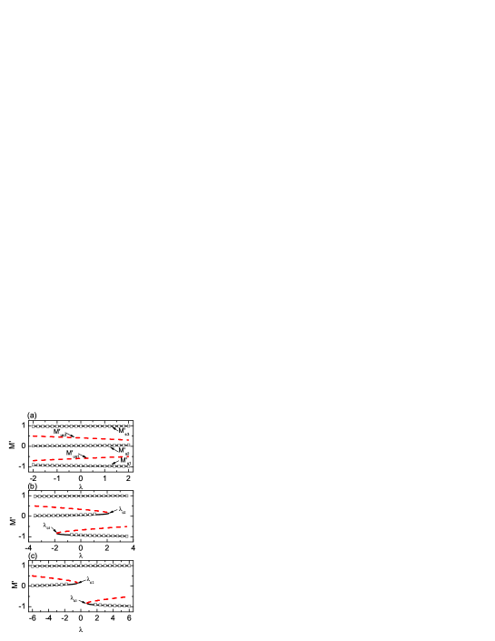
Figure 1: (color online) The solutions of $M^{\prime}$ as a function of $\lambda$ at three different $h$: $h=2$ (a), $h=3.5$ (b), and $h=6$ (c). The solid and dashed lines depict the stable and unstable solutions of $M^{\prime}$, respectively, given by the analysis Eq.(15) with a Poissonian degree distribution. The square points are given by MC simulations in $N=1000$ ER random networks. The other parameters are $\left\langle k\right\rangle=20$ and $T=5$.

To begin with, we consider a Erdös-Rényi (ER) random network with the Poissonian degree distribution $P(k)={{{{\left\langle k\right\rangle}^{k}}{e^{-}}^{\left\langle k\right\rangle}}\mathord{\left/{\vphantom{{{{\left\langle k\right\rangle}^{k}}e^{-\left\langle k\right\rangle}}{k!}}}\right.\kern-1.2pt}{k!}}$ Erdös and Rényi (1959). The average degree we use is $\left\langle k\right\rangle=20$. By numerically solving Eq.(13), we plot the solutions of $M^{\prime}$ as a function of $\lambda$ for three typical values of $h$, as shown in Fig.1. The stable and unstable solutions are depicted as the solid and dashed lines, respectively. When $h$ is small, for example $h=2$ in Fig.1(a), there are five solutions in the whole allowable range of $\lambda\in[-h,h]$, in which three of them are stable. Let $M^{\prime}_{s_{1}}$, $M^{\prime}_{s_{2}}$, and $M^{\prime}_{s_{3}}$ denote these stable solutions around $-1$, $0$, and $1$, respectively. These stable solutions give the three stable states $\uline{-1}$, $\uline{0}$, and $\uline{1}$, respectively. The other two unstable solutions, $M^{\prime}_{us_{1}}$ and $M^{\prime}_{us_{2}}$, give the two transition states from $\uline{-1}$ to $\uline{0}$ and from $\uline{0}$ to $\uline{1}$, respectively. When $h$ becomes relatively larger, as shown in Fig.1(b), the stable solution $M^{\prime}_{s_{1}}$ and the unstable $M^{\prime}_{us_{1}}$ collide and annihilate each other at $\lambda=\lambda_{c_{1}}$ via a a saddle-node bifurcation. Meanwhile, $M^{\prime}_{s_{2}}$ and the unstable $M^{\prime}_{us_{2}}$ collide and vanish at $\lambda=\lambda_{c_{2}}>\lambda_{c_{1}}$ in the same way. In this case, the property of solutions can be classified into three regions depending on the value of $\lambda$. For $\lambda<\lambda_{c_{1}}$, there are two stable solutions, $M^{\prime}_{s_{2}}$ and $M^{\prime}_{s_{3}}$, and one unstable solution $M^{\prime}_{us_{2}}$. For $\lambda>\lambda_{c_{2}}$, there are also two stable solutions and one unstable solution, but they are $M^{\prime}_{s_{1}}$ $M^{\prime}_{s_{3}}$, and $M^{\prime}_{us_{1}}$. While for $\lambda_{c_{1}}<\lambda<\lambda_{c_{2}}$, the property of solutions is the same as in Fig.1(a). With further increasing $h$, as shown in Fig.1(c), $\lambda_{c_{1}}$ shifts to a larger value, and at the same time $\lambda_{c_{2}}$ shifts to a smaller value, so that $\lambda_{c_{1}}>\lambda_{c_{2}}$. In this case, there is a single stable solution $M^{\prime}_{s_{3}}$ at $\lambda_{c_{2}}<\lambda<\lambda_{c_{1}}$.

For comparison, we have performed Monte Carlo simulations in ER random networks with network size $N=1000$ to compute the steady state values of $M^{\prime}$. The simulations start from numerous various initial configurations to sample all possible steady state values of $M^{\prime}$, where $M^{\prime}$ can be conveniently computed as $M^{\prime}={{\sum\nolimits_{i=1}^{N}{{k_{i}}{\sigma_{i}}}}\mathord{\left/{\vphantom{{\sum\nolimits_{i=1}^{N}{{k_{i}}{\sigma_{i}}}}{(\left\langle k\right\rangle N)}}}\right.\kern-1.2pt}{(\left\langle k\right\rangle N)}}$ with $k_{i}$ being the degree of node $i$. The simulation results are added into Fig.1 as shown by square points. It is clear that the simulation results are in excellent agreement with our theoretical estimations.

To get a global view, we have plotted the phase diagram in the $h\sim\lambda$ plane, as shown in Fig.2. The phase diagram is divided into four different regions according to the property of solutions of $M^{\prime}$, separating by the lines of $\lambda_{c_{1}}\sim h$ and $\lambda_{c_{2}}\sim h$. In region I, $M^{\prime}$ have five solutions: three of them are stable (corresponding to three stable states $\uline{-1}$, $\uline{0}$, and $\uline{1}$), and the others are unstable (two transition states from $\uline{-1}$ to $\uline{0}$ then to $\uline{1}$). In region II(1), $M^{\prime}$ have three solutions: two of them are stable, and the other is unstable (two stable states $\uline{-1}$, and $\uline{1}$ and one transition state). In region II(2), $M^{\prime}$ have also three solutions, but the two stable states are $\uline{0}$, and $\uline{1}$ and one transition state between them. In region III, $M^{\prime}$ has only one stable solution that corresponds to the state $\uline{1}$. Also, we have given the simulation results of $\lambda_{c_{1}}(h)$ and $\lambda_{c_{2}}(h)$, as depicted by square points in Fig.2. One can see that there exist some mismatches between the theory and simulation. This is because that near the boundaries the lifetimes of metastable states are rather short (or have very low free-energy barrier to nucleate that will be illustrated later), so that such metastable states are hard to identify in the simulations.

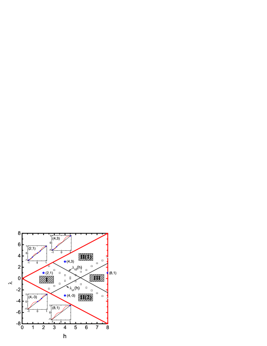
Figure 2: (color online) Phase diagram in the $h\sim\lambda$ plane. The phase diagram is divided into four different regions according to the property of solutions of $M^{\prime}$, separating by the lines of $\lambda_{c_{1}}\sim h$ and $\lambda_{c_{2}}\sim h$. In region I, $M^{\prime}$ have five solutions: three of them are stable (corresponding to three stable states $\uline{-1}$, $\uline{0}$, and $\uline{1}$), and the others are unstable (two transition states from $\uline{-1}$ to $\uline{0}$ then to $\uline{1}$). In region II(1), $M^{\prime}$ have three solutions: two of them are stable, and the other is unstable (two stable states $\uline{-1}$, and $\uline{1}$ and one transition state). In region II(2), $M^{\prime}$ have also three solutions, but the two stable states are $\uline{0}$, and $\uline{1}$ and one transition state between them. In region III, $M^{\prime}$ have only one stable solution, and the corresponding state is $\uline{1}$. Inset: Graphic solution of Eq.(15) for four typical $(h,\lambda)$ points (stars in phase diagram) chosen in four different regions. Square points give the simulation results of $\lambda_{c_{1}}(h)$ and $\lambda_{c_{2}}(h)$. The other parameters are the same as those in Fig.1.

We have also performed the calculations in Barabási-Albert (BA) scale-free networks Barabási and Albert (1999) with the same size and average degree, and found that the phase diagram is almost the same as that in ER random network (not shown here). That is, the phase diagram is not almost affected by network topology.

In Fig.3, we have schematically demonstrated the nucleation process in different regions. In region I, the system undergoes a two-step nucleation process. The first stage is the nucleating of the metastale $\uline{0}$ from $\uline{-}1$. Subsequently, in the second stage, the transition from $\uline{0}$ to $\uline{1}$ happens via the nucleating of $\uline{1}$. The free-energy barrier of the two-step nucleation are $\Delta{F_{\uline{-1}\to\uline{0}}}=N\Delta{f_{\uline{-1}\to\uline{0}}}=N(f_{M^{\prime}_{US1}}-f_{M^{\prime}_{S1}})$ and $\Delta{F_{\uline{0}\to\uline{1}}}=N\Delta{f_{\uline{0}\to\uline{1}}}=N(f_{M^{\prime}_{US2}}-f_{M^{\prime}_{S2}})$, respectively. Herein, we use the notation $f_{M^{\prime}_{*}}$ to denote free energy per node at $M^{\prime}=M^{\prime}_{*}$. In regions II(1), since the state $\uline{0}$ is no longer present, nucleation happens via a one-step process directly from $\uline{-1}$ to $\uline{1}$. The resulting free-energy barrier is $\Delta{F_{\uline{-1}\to\uline{1}}}=N\Delta{f_{\uline{-1}\to\uline{1}}}=N(f_{M^{\prime}_{US1}}-f_{M^{\prime}_{S1}})$. In region II(2), since the state $\uline{-1}$ ceases to exist, nucleation also proceeds by one-step process from $\uline{0}$ to $\uline{1}$, and the corresponding free-energy barrier is $\Delta{F_{\uline{0}\to\uline{1}}}$. In region III, the only stable state is $\uline{1}$ and the nucleation is thus irrelevant.

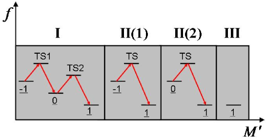
Figure 3: (color online) Schematic plot for nucleation and growth in different regions. In region I, nucleation from $\uline{-1}$ to $\uline{1}$ proceeds in a two-step process via an intermediate metastable state $\uline{0}$. In both regions II(1) and II(2), nucleation proceeds in a one-step process. In region III, the only state $\uline{1}$ is stable and thus nucleation is irrelevant.

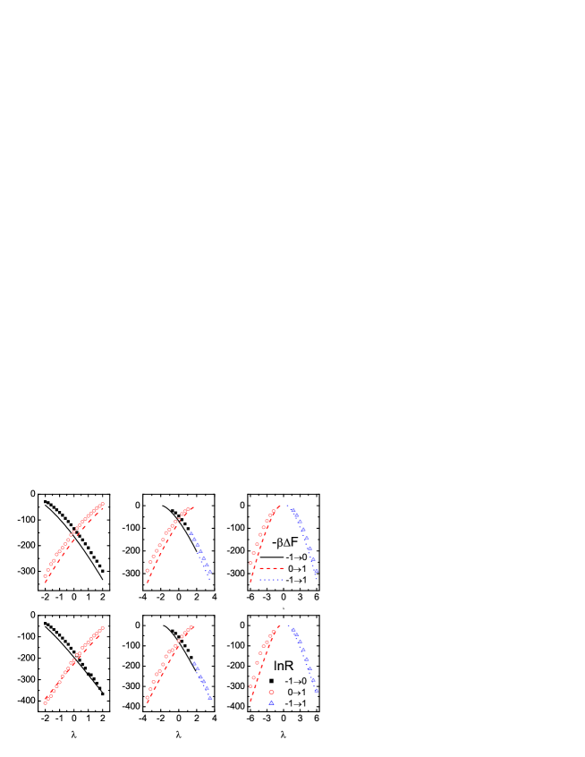
Figure 4: (color online) The free energy barrier $-\beta\Delta F$ and the logarithm of rate of nucleation $\ln R$, obtained from the HMF analysis (lines) and FFS simulations (symbols), as a function of $\lambda$ at three different $h$: $h=2$, $3.5$, $6$ (from left to right). Top and bottom panels show the results in ER networks and BA networks, respectively. The other parameters are the same as those in Fig.1.

Since nucleation rate $R$ is exponentially dependent on $-\beta\Delta F$, $R\sim\exp(-\beta\Delta F)$, at the top and bottom panels of Fig.4 we show that $-\beta\Delta F$ as a function of $\lambda$ at three typical different $h$: $h=2$, $3.5$, $6$ (from left to right) in ER networks (top panels) and BA networks (bottom panels), respectively (shown by lines). To validate the analytical results, computer simulation for calculating nucleation rate is desirable.

However, nucleation is an activated process that occurs extremely slow, and brute-force simulation for observing nucleation process is thus prohibitively expensive. To overcome this difficulty, we will employ a recently developed simulation method, forward flux sampling (FFS) Allen et al. (2005); Valeriani et al. (2007). This method allows us to calculate nucleation rate and determine the properties of ensemble toward nucleation pathways. This method uses a series of interfaces in phase space between the initial and final states to force the system from the initial state $A$ to the final state $B$ in a ratchet-like manner. Before the simulation begins, an order parameter $r$ is first defined, such that the system is in state $A$ if $r<r_{0}$ and it is in state $B$ if $r>r_{n}$. A series of nonintersecting interfaces $r_{i}$ ($0<i<n$) lie between states $A$ and $B$, such that any path from $A$ to $B$ must cross each interface without reaching $r_{i+1}$ before $r_{i}$. The algorithm first runs a long-time simulation which gives an estimate of the flux $\bar{\Phi}_{A,0}$ escaping from the basin of $A$ and generates a collection of configurations corresponding to crossings of interface $r_{0}$. The next step is to choose a configuration from this collection at random and use it to initiate a trial run which is continued until it either reaches $r_{1}$ or returns to $r_{0}$. If $r_{1}$ is reached, store the configuration of the end point of the trial run. Repeat this step, each time choosing a random starting configuration from the collection at $r_{0}$. The fraction of successful trial runs gives an estimate of of the probability of reaching $r_{1}$ without going back into $A$, $P\left({r_{1}|r_{0}}\right)$. This process is repeated, step by step, until $r_{n}$ is reached, giving the probabilities $P\left({r_{i+1}|r_{i}}\right)$ ($i=1,\cdots,n-1$). Finally, we get the nucleation rate $R$ from $A$ to $B$ as

$$R=\bar{\Phi}_{A,0}P\left({r_{n}|r_{0}}\right)=\bar{\Phi}_{A,0}\prod\nolimits_{i=0}^{n-1}{P\left({r_{i+1}|r_{i}}\right)},$$ (17)

where $P\left({r_{n}|r_{0}}\right)$ is the probability that a trajectory crossing $r_{0}$ in the direction of $B$ will eventually reach $B$ before returning to $A$.

For comparison, we have also added the simulation results to Fig.4 (shown by symbols). On one hand, the analytical results are in well agreement with the simulation ones. On the other hand, the results in ER random networks and in BA scale-free networks are qualitatively the same.

For $h=2$, nucleation is a two-step process in the whole allowable range of $\lambda$, and the corresponding nucleation rates are $R_{\uline{-1}\to\uline{0}}$ and $R_{\uline{0}\to\uline{1}}$, respectively. As $\lambda$ increases, $R_{\uline{-1}\to\uline{0}}$ decreases monotonically, but $R_{\uline{0}\to\uline{1}}$ increases monotonically. In this case, the total nucleation rate $R$ is expressed as $R=(R_{\uline{-1}\to\uline{0}}^{-1}+R_{\uline{0}\to\uline{1}}^{-1})^{-1}$. It can be seen that $R$ is dominantly determined by the smaller of $R_{\uline{-1}\to\uline{0}}$ and $R_{\uline{0}\to\uline{1}}$. Therefore, there exists a maximal $R$ at $\lambda=\lambda_{opt}$ where $R_{\uline{-1}\to\uline{0}}$ and $R_{\uline{0}\to\uline{1}}$ intersect. Here, $\lambda_{opt}\simeq 0.1$ for ER random networks and $\lambda_{opt}\simeq 0.2$ for BA scale-free networks that are robust to different $h$. For $h=3.5$, nucleation is a two-step process in a certain range of $\lambda$ around zero, while in other range nucleation becomes a one-step process. The resulting total nucleation rate has also a maximum at $\lambda=\lambda_{opt}$. For $h=6$, nucleation is a one-step process and the corresponding nucleation rate increases as $\lambda$ gradually approaches zero until nucleation becomes irrelevant when $\lambda$ crosses the line of $\lambda_{c_{1}}(h)$ or $\lambda_{c_{2}}(h)$.

IV Conclusion

In conclusion, we have studied the nucleation of the three-state BC model on complex networks. By using the heterogeneous mean-field theory and simulations, we have found that there exist four distinct regions with different nucleation scenarios depending on the model’s parameters: the external field $h$ and the chemical potential $\lambda$. For a small $h$, or for a moderate $h$ and simultaneously a small $\left|\lambda\right|$, the system goes through a two-step nucleation process from $\uline{-1}$ configuration to $\uline{0}$ configuration and then to $\uline{1}$ configuration. For a moderate $h$ or a large $h$ and simultaneously a large $\left|\lambda\right|$, nucleation is a one-step process without an intermediate metastable configuration directly from $\uline{-1}$ configuration to $\uline{1}$ configuration or directly from $\uline{0}$ configuration to $\uline{1}$ configuration depending on the sign of $\lambda$. For a large $h$ and simultaneously a small $\left|\lambda\right|$, the metastability of the system vanishes and nucleation is thus irrelevant. Moreover, we have calculated the nucleation rates and found that in the two-step nucleation region there exists a maximum for the total nucleation rate. All the results are demonstrated in ER random networks and in BA scale-free networks and are qualitatively the same for different network topologies. Quantitatively, the optimal $\lambda_{opt}$ at which the total nucleation rate is maximal in ER random networks is less than that in more heterogeneous BA scale-free networks.