Quantum-Limited Spectroscopy

Abstract

Spectroscopy has an illustrious history delivering serendipitous discoveries and providing a stringent testbed for new physical predictions, including applications from trace materials detection, to understanding the atmospheres of stars and planets, and even constraining cosmological models. Reaching fundamental-noise limits permits optimal extraction of spectroscopic information from an absorption measurement. Here we demonstrate a quantum-limited spectrometer that delivers high-precision measurements of the absorption lineshape. These measurements yield a ten-fold improvement in the accuracy of the excited-state (6P_1/2) hyperfine splitting in Cs, and reveals a breakdown in the well-known Voigt spectral profile. We develop a theoretical model that accounts for this breakdown, explaining the observations to within the shot-noise limit. Our model enables us to infer the thermal velocity-dispersion of the Cs vapour with an uncertainty of 35ppm within an hour. This allows us to determine a value for Boltzmann’s constant with a precision of 6ppm, and an uncertainty of 71ppm.

Spectroscopy is a vital tool for both fundamental and applied studies. It is critical to drive improvements in both precision and accuracy in order to gain maximum physical information about the quantum absorbers – even as they are perturbed by the probe. The immediate motivation for this work has arisen out of a call to the scientific community to develop new techniques to re-measure Boltzmann’s constant, $k_{\textrm{B}}$, in preparation for a redefinition of the kelvin Fellmuth et al. (2006); however, advances in absorption lineshape measurement and theory will find applications in accurate gas detection and monitoring Stewart et al. (2011), studies of planetary atmospheres Drossart (2005), thermometry in tokamaks Koch et al. (2012) and understanding distant astrophysical processes Grefenstette et al. (2014); Hayato et al. (2010). The accurate measurement of the natural linewidth and transition frequencies, which can be directly related to the atomic lifetime, level structure and transition probabilities, is important for testing atomic physics Wood et al. (1997); Jönsson et al. (1996); Brage et al. (1994).

Here we present measurements of a transmission lineshape of cesium (Cs) vapor with a quantum-limited transmission uncertainty of 2 ppm in a 1 second measurement, which is to our knowledge, a factor of 16 times superior to anything previously demonstrated Moretti et al. (2013). This extreme precision allows us to directly detect subtle lineshape perturbations that have not been previously observed. This observation prompted the development of a theoretical model, which now allows us to discriminate between the internal atomic state dynamics and their external motional degrees. Using the model we are able to estimate the velocity dispersion of the atoms with a precision (standard error) of 53 ppm during a single line scan, taking $\sim 30$ seconds. This is consistent with the the sample standard deviation (also 53 ppm) over multiple scans, demonstrating the excellent reproducibility of the spectrometer. The measurement precision averages down to 3.7 ppm after 200 scans. These values are $\sim 7$ times better than the previous best results Lemarchand et al. (2010); Djerroud et al (2009); Moretti et al. (2013), and also yield a 10-fold improvement in the uncertainty of the excited state hyperfine splitting in Cs Steck (2009); Udem et al. (1999). Our measurement of the homogenous broadening component of the line shape has a precision within a factor of two of the best ever measurement of natural linewidth. Modest improvements in the probe laser performance would deliver a new result for the excited state lifetime of Cs in a system that is experimentally and theoretically much simpler than that typically used for lifetime studies Rafac et al. (1999); Amini and Gould (2003).

[]schematic11(15cm) [lb]122,26;P [lb]127,5;M [lb]136,23;C [t]106,24;OC [lb]100,6;AOM [lb]83,4;Blocker [bl]85.5,23;GT [lb]78,24;W [lb]25,10.5;Cs Cell [lb]29,21;SPRT 1 [lb]43,9.8;SPRT 2 [lb]45,2;Shield [lb]1,6;PDA [lb]66,26;PDB

Figure 1: Schematic of a high-accuracy linear absorption spectrometer based on a probe laser (P) that is tightly locked at a tunable frequency difference away from a master laser (M), which is itself stabilised to an atomic transition in Cs. The frequency stability of the master laser is compared to a reference frequency provided by an optical frequency comb (C). The probe is spectrally filtered with an optical cavity (OC), and actively power-stabilised with an acousto-optic modulator (AOM). The probe is then divided with high-precision into two beams using a Glan-Taylor (GT) polarizing prism followed by a Wollaston beamsplitter (W). One beam passes through a Cs cell embedded inside a thermal and magnetic shield and is measured by photodiode A (PD A); the other beam is measured directly by photodiode B (PD B). Temperature and thermal gradients are measured independently with calibrated standard platinum resistance thermometers (SPRTs).

At thermal equilibrium, the velocity distribution of atomic absorbers in a vapour cell is related to the temperature through the Boltzmann distribution. This simple and fundamental relationship forms an excellent foundation for a type of primary thermometry known as Doppler broadening thermometry (DBT) Bordé (2005, 2009). DBT differs from the current leading technique for primary thermometry, which measures the temperature-dependent speed of sound in a noble gas contained in a well-characterized acoustic resonator. Until recently, the best determination of $k_{\textrm{B}}$ was made in 1988 with a total uncertainty of 1.7 parts-per-million (ppm) Moldover et al. (1988). Refinements to this technique over the last twenty years have reduced its uncertainty to the 1 ppm level Pitre et al. (2011); de Podesta et al. (2013), improving the uncertainty in the CODATA-recommended value for $k_{\textrm{B}}$ from 1.8 ppm (CODATA-02) to 0.91 ppm (CODATA-10). Despite these superb measurements, it is important that different techniques are employed to measure $k_{\textrm{B}}$ to reduce the possibility of underestimating systematic uncertainties that may be inherent to any single technique Cohen and DuMond (1965).

The DBT approach is one of the most theoretically transparent of the new approaches to primary thermometry. The spectrum of a gas sample is measured with high precision, and a theoretical model is fitted to the measured data. If the model includes all of the relevant physics then one can accurately extract the contribution to spectral broadening arising solely from the thermal distribution of atomic/molecular speeds. Ammonia probed by a frequency-stabilized CO₂ laser at 1.34 $\mu$m was the first thermometric substance employed in a DBT experiment Daussy et al (2007). Subsequently, an extended-cavity diode laser at 2 $\mu$m was used to probe a ro-vibrational transition of CO₂ Casa et al (2008). In these first experiments, the line-shape was assumed to be a Gaussian or a Voigt profile (a Gaussian convolved with a Lorentzian). Since 2007, with the ambitious goal of approaching 1 ppm accuracy, substantial experimental and theoretical improvements have been made to DBT using ammonia Triki et al. (2012); Lemarchand et al. (2012), oxygen Cygan et al. (2010), ethyne Hald et al. (2011), and water Gianfrani (2012). However, one key challenge peculiar to molecular absorbers is the need to account for complex collisional effects on the line shape Lemarchand et al. (2012). We avoid this by using a dilute atomic vapour Truong et al. (2012, 2011) with a strong dipole transition for which a tractable, microscopic theory has been developed Stace et al. (2012); Stace and Luiten (2010).

The spectrometer is pictured in Fig. 1. The probe laser is spectrally and spatially filtered using a combination of an optical cavity of moderate finesse ($\mathcal{F}\approx 305$) and single-mode fibre. This reduces the spontaneous emission content of the probe beam from 1.6% to below 0.01%. It is then delivered into a vacuum chamber in which the vapour cell is mounted in a thermal and magnetic shield. The temperature of the shield can be controlled to a few millikelvin and gradients are suppressed to the same level. The light is split into two output signals using a combination of a Glan-Taylor polarising prism and Wollaston beam-splitter. The ratio of powers in the output beams is stable to better than $10^{-6}$. One output directly illuminates a photodiode to give the incident power, whilst the other passes through the vapour cell and is then detected. The ratio of these photodiode signals gives us the transmission ratio, $\mathcal{T}$. The incident power is actively controlled while the frequency of the incident light is set to an absolute accuracy of 2 kHz. The temperature of the vapour cell is monitored directly using a calibrated capsule-type standard platinum resistance thermometer (CSPRT), allowing us to quantify the performance of our Doppler thermometer. Further technical details about the apparatus are given in the supplementary information (SI).

We measure the transmission through the vapour cell as the probe laser frequency scans across the Cs D1 transition (6S_1/2 – 6P_1/2), shown in Fig. 2(a). The relative noise in the measurement of the atomic transmission is just 2 ppm in a 1 s measurement (at the highest optical powers used). The two dips seen on Fig. 2(a) come from the hyperfine splitting in the excited state and our excellent signal-to-noise ratio enables us to determine this splitting to be $f_{\textrm{HFS}}=1167.716(3)\textrm{ MHz}$ consistent with previous measurements ($f_{\textrm{HFS}}=$1167.680(30) MHz Steck (2009); Udem et al. (1999)), but 10 times more accurate.

The absorption line-shape, $\mathcal{T}_{\textrm{at}}(f)$, of an atomic transition with a rest-frame transition frequency $f_{0}$, is given by a convolution of the natural (half) linewidth $\Gamma_{L}=1/(4\pi\tau)$ due to the finite lifetime $\tau$ of the transition, with a Gaussian distribution having a $e^{-1}$-width $\Gamma_{D}=f_{0}\sqrt{2k_{\textrm{B}}T/(m_{\textrm{Cs}}c^{2})}$ due to Doppler broadening of atoms of mass $m$ at temperature $T$. By fitting a line-shape to the measured transmission data, with $\Gamma_{D}^{\textrm{fit}}$ as a fitting parameter, we extract the Doppler component, from which we infer the temperature. Systematic errors in $\Gamma_{D}^{\textrm{fit}}$ are quantified by converting the independent PRT temperature measurements into an expected Doppler width, $\Gamma_{D}^{\textrm{PRT}}$, using the CODATA values for $k_{\textrm{B}}$ and $m_{\textrm{Cs}}$, which we compare with $\Gamma_{D}^{\textrm{fit}}$.

[]trans(8.6cm)[t]0,42;(a) []res4bAndreGreenVoigtOnlyBlue1CorrNoetalons(8.6cm)[t]0,42;(b) []etalon2327(8.6cm)[t]0,45;(c) []res4dAndreLightBlue1Corr0EtalonDarkBlue1Corr6EtalonRed2Corr6Etalon(8.6cm)[t]0,55;(d)

Figure 2: (a) Measured transmission at 296 K for the highest intensity, $I/I_{\textrm{sat}}=0.0028$, averaged over 200 scans [points] and theory [solid]. (b) Residuals including Voigt only [dark-green] and first-order correction [light-blue]. (c) Etalon pre-factor, Eq. 1, with 6 etalons [solid] and data divided by second-order power-corrected Voigt profiles [points], assuming $\Gamma_{L}=2.327$ MHz. (d) Residuals after including first-order correction with 0 etalons [light-blue] and 6 etalons [dark-blue], and second-order with 6 etalons [dotted-red].

If the natural lineshape of the transition is a Lorentzian, then the resulting convolution is the well-known Voigt profile, which is commonly used to model dipole resonances. However, our extremely low-noise transmission measurements reveal deviations from the Voigt profile. Some of these deviations are technical in origin e.g. instrumental broadening due to the lineshape of the probing laser, residual spontaneous emission from the probe laser, unwanted optical etalons, and photodetector linearity; however, there is an important fundamental effect resulting from frequency-dependent optical pumping, which perturbs the atomic natural line-shape away from a Lorentzian. All of these effects, whether technical or fundamental, cause systematic perturbations to the line shape, and must be taken into account to model the lineshape accurately.

To demonstrate these deviations, we fit a model consisting of two Voigt profiles separated by $f_{\textrm{HFS}}$, to the raw transmission data shown Fig. 2(a). The residuals of this Voigt-only fit have characteristic M-shaped features near resonance, with amplitude $\sim 200$ ppm at the highest probe powers, as shown in the green trace in Fig. 2(b). These features demonstrate the breakdown of the Voigt profile, indicating additional, unaccounted physics, which causes a spurious linear dependence of $\Gamma_{D}^{\textrm{fit}}$ on probe intensity, as shown in the green curve on Fig. 3. In what follows, we describe how we sequentially include additional physics in our transmission model to remove these, and other, systematic effects, leaving only the shot-noise limit of our detection apparatus.

In earlier work we showed that the M-shaped features in Fig. 2(b) arise from atomic population dynamics induced by the probe laser, which are significant even at exceedingly low intensities Stace et al. (2012). We subsequently calculated corrections to the Voigt profile up to linear-order in the probe intensity Stace and Luiten (2010), to account for optical pumping. Including these first-order intensity-dependent correction in our model suppresses the features substantially, as shown in the blue trace in Fig. 2(b).

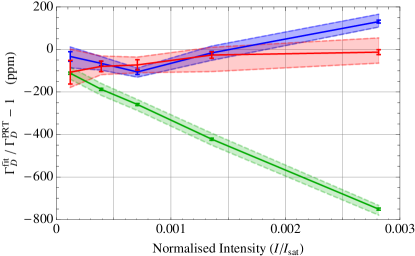
Figure 3: Fractional deviation between the fitted Doppler width and that inferred from PRT temperature measurements at 296 K. Green points are fits using the power-independent Voigt-only profile. Blue points are fits using the first-order intensity-dependent correction. Red points are fits using the second-order intensity-dependent correction. Solid curves are fits using our central estimate of $\bar{\Gamma}_{L}=2.327$ MHz; dashed curves are for $\Gamma_{L}=2.320$ MHz (upper) and $\Gamma_{L}=2.334$ MHz (lower) representing $\bar{\Gamma}_{L}\pm\sigma_{\Gamma_{L}}$: the shaded regions indicates the sensitivity of $\Gamma_{D}^{\textrm{fit}}$ to $\Gamma_{L}$ in this range. Error bars represent standard errors of fits to the average of 200 scans for fixed $\Gamma_{L}$.

Far from the resonances, oscillations are evident in Fig. 2(b). These arise from low-finesse etalons in the optics used to deliver the light to the atoms. The dominant etalon has an amplitude around 40 ppm, corresponding to interference between surfaces with power reflectivities of $\lesssim 10^{-9}$. Although obviously technical in nature, reducing the size of etalons beyond this already fantastically low level is an experimental challenge. Instead, we include etalons in our transmission model, so that the total transmission is given by $\mathcal{T}=\mathcal{T}_{\textrm{at}}\mathcal{T}_{\textrm{e}t}$, where $\mathcal{T}_{\textrm{e}t}$ includes $n$ etalons and a slowly-varying quadratic background:

$$\mathcal{T}_{\textrm{e}t}(f)=\frac{\alpha+\beta f+\gamma f^{2}}{\prod_{j=1}^{n}\big{(}1+a_{j}\sin(2\pi f/f_{j}+\phi_{j})\big{)}}.$$ (1)

Etalons are of particular concern for DBT since they introduce systematic errors in $\Gamma_{D}^{\textrm{fit}}$. We note that it is only because of our extreme transmission sensitivity that these features are revealed, and thus give the opportunity to suppress this systematic error.

We add etalons to the model until the residuals far from resonance are consistent with a white-noise background. In practice, it is necessary to include up to $n=6$ etalons for high power scans, with the smallest resolved etalons having amplitude $\sim 7$ ppm. The solid curve in Fig. 2(c) shows $\mathcal{T}_{\textrm{e}t}$ for the highest power data; the points show the raw transmission data divided by the fitted $\mathcal{T}_{\textrm{a}t}$, demonstrating that $\mathcal{T}_{\textrm{e}t}$ is uncorrelated with the atomic transmission profile shown in Fig. 2(a).

Source	$u_{r}(k_{B})$ (ppm)
Statistical (from Fig. 4)	5.8
Lorentz Width ($\Gamma_{L}^{\textrm{fit}}$)a	65
Lorentz Width ($\Gamma_{L}^{\textrm{ind}}$)b	190
Laser Gaussian noise	16
Optical pumping	15
Etalons (misidentification)	15
Etalons (unresolved)	3
Spontaneous Emission	3.6
Temperature	1.9
Temp. Gradient	1.2
PD Linearity	1
Zeeman Splitting	$<$1.2
Total (fit $\Gamma_{L}$)	71
Total (independent $\Gamma_{L}$)	191

Table 1: Error budget for the determination of the Boltzmann constant at 296 K. Optical pumping shifts are reported at $I/I_{sat}=3\times 10^{-3}$ assuming second-order corrections to the Voigt profile. ^aEstimated from fits to scan data with free LW. ^bEstimated from published uncertainty in Cs lifetime, plus uncertainty in the independent estimate of the laser linewidth. $u_{r}$ denotes fractional uncertainty.

The dark blue trace in Fig. 2(d) includes first-order power-dependent corrections, and $6$ etalons. Away from resonance, the residuals are then consistent with the noise-floor of our apparatus. However, around the deepest resonance we observe $\sim 10$ ppm features. To eliminate these we include second-order intensity-dependent corrections to the Voigt profile (see SI):

$$\mathcal{T}^{(i)}_{\textrm{at}} = e^{-pV_{\nu}(\Delta)}\Big{(}1+q_{1}{(e^{-pV_{\nu}(\Delta)}-1)V_{\nu}^{(2)}(\Delta)}/{V_{\nu}(\Delta)}$$ (2)

$${}\hphantom{e^{-pV(}}+q_{2}\big{(}{(e^{-pV_{\nu}(\Delta)}-1)V_{\nu}^{(2)}(\Delta)}/{V_{\nu}(\Delta)}\big{)}^{2}$$

$${}\hphantom{e^{-pV(}}+q_{3}{(e^{-2pV(\Delta,\nu)}-1)V_{\nu}^{(3)}(\Delta)}/{V_{\nu}(\Delta)}\Big{)},$$

where $\nu=\Gamma_{D}/\Gamma_{L}$, $\Delta$ is the detuning from the resonance, and the generalised Voigt profile is given by $V^{(n)}_{\nu}(\Delta)=\pi^{-3/2}\int_{-\infty}^{\infty}dx\,{e^{-{(\Delta-x)^{2}}/{\nu^{2}}}}{(1+{{x^{2}}})^{-n}},$ and the conventional Voigt profile is $V_{\nu}(\Delta)=V^{(1)}_{\nu}(\Delta)$. For a cell of length $L$ with linear absorption coefficient $\alpha$, the optical depth on resonance is $p=\alpha L$, $q_{1}\propto I$ is the linear intensity-dependent coefficient Stace et al. (2012), and $q_{2,3}\propto I^{2}$ are quadratic intensity-dependent coefficients.

The red dotted trace in Fig. 2(d) shows the residuals after including second-order intensity corrections. The residuals are suppressed to $\sim 2$ ppm, consistent with the detection noise floor, giving confidence that the transmission model accounts for systematic effects.

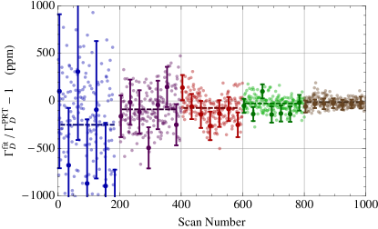
Figure 4: Deviation between $\Gamma_{D}^{\textrm{fit}}$ (using second-order intensity correction) and $\Gamma_{D}^{\textrm{PRT}}$, for each scan at 296 K, with $\Gamma_{L}=2.327$ MHz. Colours and vertical lines demark different incident intensities (lowest at left, corresponding to normalised intensities in Fig. 1). Dashed lines are the mean of the corresponding set of scans, error bars are the estimated parameter error ($\pm 1\sigma$) for each selected scan, and are consistent with sample standard deviation. Etalons are included in each fit, with parameters fixed by fits to the average of all scans within a power level, i.e. etalon parameters are not free to vary within a particular power level.

Figure 3 compares the fractional deviation between $\Gamma_{D}^{\textrm{fit}}$ and $\Gamma_{D}^{\textrm{PRT}}$ as a function of incident intensity for the three possible models for the atomic line shape: Voigt-only (green), first-order (blue) and second-order (red) intensity-dependent corrections. Naturally, the true $\Gamma_{D}$ should be intensity independent. The simplest Voigt-only theory clearly exhibits a linear intensity-dependence, leading to $\sim 750$ ppm discrepancy even at intensities as low as $I/I_{\textrm{sat}}=2.8\times 10^{-3}$ where $I_{\textrm{sat}}=2.5$ mW/cm² is the saturation intensity for the transition Steck (2009). From Stace and Luiten (2010), we expect the first-order correction to have a residual quadratic dependence on intensity, which is consistent with the blue curve on Fig. 3. Finally, the second-order correction (red curve) is seen to suppress all intensity dependence to below the measurement precision. The simultaneous removal of all systematic features from the residuals together with the elimination of intensity-dependence in the recovered $\Gamma_{D}^{\textrm{fit}}$ gives a high degree of confidence that all relevant physics is properly included in the theoretical model.

Thermometry: In this section we demonstrate the power of our spectroscopic technique by applying it to the problem of primary thermometry, and determine a value for Boltzmann’s constant using atomic spectroscopy.

The atomic vapour is brought to thermal equilibrium at a chosen temperature by suspending it within a thermal isolator with an independent means for temperature measurement accurate to 0.55 mK (1.9 ppm). After systematically removing the effects of optical pumping and etalons, the largest source of uncertainty in $\Gamma_{D}^{\textrm{fit}}$ comes from uncertainty in $\Gamma_{L}$. We obtain a value for $\Gamma_{L}$ directly by fitting it to the data, which gives $\Gamma_{L}^{\textrm{fit}}=2.327(7)$ MHz. This is consistent with, but also more precise than, an independent estimate, $\Gamma_{L}^{\textrm{ind}}=2.331(19)$ MHz, given by the sum of the natural linewidth of the Cs $6P_{1/2}$ level, $\Gamma_{L}^{\textrm{at}}=2.287(6)$ MHz Steck (2009), and the laser linewidth, $\Gamma_{L}^{\textrm{las}}=0.044(18)$ MHz. From Fig. 3 we estimate that a 1 kHz change in $\Gamma_{L}$ leads to $\sim 5$ ppm change in $\Gamma_{D}^{\textrm{fit}}$, so that the 6.5 kHz uncertainty in $\Gamma_{L}$ contributes 32.5 ppm uncertainty in $\Gamma_{D}^{\textrm{fit}}$ [65 ppm in $u_{r}(k_{\textrm{B}})$]. We note that if the probe laser linewidth were decreased to the kilohertz level, then our measurement would yield a state-of-the-art value for the excited state lifetime of Cs.

We now briefly describe additional sources of uncertainty, which are quantified in Table 1 (see SI for a comprehensive description). Statistical error arising from the scatter in Fig. 4 contributes 2.9 ppm to $u_{r}(\Gamma_{D}^{\textrm{fit}})$ [5.8 ppm to $u_{r}(k_{\textrm{B}})$]. This is also consistent with the estimated standard error for each point in Fig. 4, shown as error bars. The probe laser has gaussian noise of width 0.88(39) MHz, contributing 8 ppm to $u_{r}(\Gamma_{D}^{\textrm{fit}})$ [16 ppm to $u_{r}(k_{\textrm{B}})$]. Residual effects of optical pumping after second-order power corrections contribute 7.5 ppm to $u_{r}(\Gamma_{D}^{\textrm{fit}})$, [15 ppm to $u_{r}(k_{\textrm{B}})$]. Misidentification of etalon parameters contributes $7.5$ ppm to $u_{r}(\Gamma_{D}^{\textrm{fit}})$, [15 ppm to $u_{r}(k_{\textrm{B}})$]. Possible unresolved etalons contribute 3 ppm to $u_{r}(k_{\textrm{B}})$. Residual spontaneous emission from the laser, after filtering by the optical cavity, contributes 3.6 ppm to $u_{r}(k_{\textrm{B}})$.

To determine a value for $k_{\textrm{B}}$, we take a weighted mean of $\Gamma_{D}^{\textrm{fit}}/\Gamma_{D}^{\textrm{PRT}}$ extracted from fits using all the second-order corrected data shown on Fig. 3 (red points). We find $k_{\textrm{B}}=1.380\,545(98)\times 10^{-23}$ J/K, where the 71 ppm uncertainty is calculated in Table 1. This is consistent with the recommended CODATA value of $1.380\,648\,8(13)\times 10^{-23}$ J/K.

In conclusion, we have developed an atomic absorption spectrometer that operates with a transmission measurement precision of just 2 ppm. This has revealed several new phenomena. In combination with a theory that correctly treats the interaction between light and an effusive vapour we are able to explain all of the observed effects to a level of precision never before demonstrated. The power of our technique is demonstrated by measuring the line-shape parameters of a gas at thermal equilibrium. Our reproducibility is exactly consistent with the quantum-limits of measurement Stace (2010) which gives us confidence that we have captured all of the relevant physics.

With our unprecentented sensitivity, we have measured the transmission spectrum of Cs at 895 nm at the shot-noise limit. From these measurements, we derived a value for Boltzmann’s constant with an uncertainty of 71 ppm, which is consistent with the recommended CODATA value, and the hyperfine frequency splitting of the $6^{2}P_{1/2}$ level with an uncertainty ten times better than ever previously reported:

$$k_{\textrm{B}} = 1.380\,545(98)\times 10^{-23}\textrm{ J/K}$$

$$f_{\textrm{HFS}} = 1167.716(3)\textrm{ MHz.}$$

Our current performance permits a measurement of the Boltzmann constant with a precision of 6 ppm after only a few hours of data acquisition. Our total uncertainty is dominated by the imprecision in the literature value of the excited state lifetime of the Cs D1 transition (known to 0.26% Steck (2009)). A future experiment designed to further reduce the amplitude of etalons, and using a more broadly tuneable ($\sim 30$ GHz) and higher power probe laser with sub-kHz linewidth would eliminate probe laser effects, allow better estimation of etalon contamination, and lower the contribution of optical pumping. This opens the door to the best measurement of the Cs D1 transition lifetime, and a ppm-level measurement of $k_{\textrm{B}}$ thus making an important contribution to efforts to redefine the kelvin.

The authors wish to thank the NIST Precision Measurement Grants Program, the Australian Research Council through the CE110001013, FT0991631 and DP1094500 grants for funding this work. The authors also wish to acknowledge the South Australian Government who have provided generous financial support through the Premier’s Science and Research Fund. We thank Michael Moldover and Greg Strouse of NIST, and Mark Ballico from NMI Australia, for their contributions to the SPRT thermometry.

References

- Fellmuth et al. (2006) B. Fellmuth, C. Gaiser, and J. Fischer, Measurement Science and Technology 17, R145 (2006).
- Stewart et al. (2011) G. Stewart, W. Johnstone, J. R. P. Bain, K. Ruxton, and K. Duffin, J. Lightwave Technol. 29, 811 (2011).
- Drossart (2005) P. Drossart, Comptes Rendus Physique 6, 817 (2005).
- Koch et al. (2012) J. A. Koch, R. E. Stewart, P. Beiersdorfer, R. Shepherd, M. B. Schneider, A. R. Miles, H. A. Scott, V. A. Smalyuk, and W. W. Hsing, Review of Scientific Instruments 83, 10E127 (2012).
- Grefenstette et al. (2014) B. Grefenstette, F. Harrison, S. Boggs, S. Reynolds, C. Fryer, K. Madsen, D. Wik, A. Zoglauer, C. Ellinger, D. Alexander, et al., Nature 506, 339 (2014).
- Hayato et al. (2010) A. Hayato, H. Yamaguchi, T. Tamagawa, S. Katsuda, U. Hwang, J. P. Hughes, M. Ozawa, A. Bamba, K. Kinugasa, Y. Terada, A. Furuzawa, H. Kunieda, and K. Makishima, The Astrophysical Journal 725, 894 (2010).
- Wood et al. (1997) C. S. Wood, S. C. Bennett, D. Cho, B. P. Masterson, J. L. Roberts, C. E. Tanner, and C. E. Wieman, Science 275, 1759 (1997).
- Jönsson et al. (1996) P. Jönsson, A. Ynnerman, C. Froese Fischer, M. R. Godefroid, and J. Olsen, Phys. Rev. A 53, 4021 (1996).
- Brage et al. (1994) T. Brage, C. F. Fischer, and P. Jönsson, Phys. Rev. A 49, 2181 (1994).
- Moretti et al. (2013) L. Moretti, A. Castrillo, E. Fasci, M. D. De Vizia, G. Casa, G. Galzerano, A. Merlone, P. Laporta, and L. Gianfrani, Phys. Rev. Lett. 111, 060803 (2013).
- Lemarchand et al. (2010) C. Lemarchand, K. Djerroud, B. Darquié, O. Lopez, A. Amy-Klein, C. Chardonnet, C. Bordé, S. Briaudeau, and C. Daussy, International Journal of Thermophysics 31, 1347 (2010).
- Djerroud et al (2009) K. Djerroud et al, Comptes Rendus Physique 10, 883 (2009).
- Steck (2009) D. Steck, “Cesium D line data (unpublished) http://steck.us/alkalidata,” (2009).
- Udem et al. (1999) T. Udem, J. Reichert, R. Holzwarth, and T. Hänsch, Physical Review Letters 82, 3568 (1999).
- Rafac et al. (1999) R. J. Rafac, C. E. Tanner, A. E. Livingston, and H. G. Berry, Phys. Rev. A 60, 3648 (1999).
- Amini and Gould (2003) J. M. Amini and H. Gould, Phys. Rev. Lett. 91, 153001 (2003).
- Bordé (2005) C. Bordé, Phil. Trans. of the Royal Society A 363, 2177 (2005).
- Bordé (2009) C. Bordé, Comptes Rendus Physique 10, 866 (2009).
- Moldover et al. (1988) M. Moldover, J. Trusler, T. Edwards, J. Mehl, and R. Davis, Physical Review Letters 60, 249 (1988).
- Pitre et al. (2011) L. Pitre, F. Sparasci, D. Truong, A. Guillou, L. Risegari, and M. Himbert, International Journal of Thermophysics 32, 1825 (2011).
- de Podesta et al. (2013) M. de Podesta, R. Underwood, G. Sutton, P. Morantz, P. Harris, D. F. Mark, F. M. Stuart, G. Vargha, and G. Machin, Metrologia 50, 354 (2013).
- Cohen and DuMond (1965) E. R. Cohen and J. W. M. DuMond, Rev. Mod. Phys. 37, 537 (1965).
- Daussy et al (2007) C. Daussy et al, Phys. Rev. Lett. 98, 250801 (2007).
- Casa et al (2008) G. Casa et al, Phys. Rev. Lett. 100, 200801 (2008).
- Triki et al. (2012) M. Triki, C. Lemarchand, B. Darquié, P. L. T. Sow, V. Roncin, C. Chardonnet, and C. Daussy, Phys. Rev. A 85, 062510 (2012).
- Lemarchand et al. (2012) C. Lemarchand, M. Triki, B. Darquié, P. L. T. Sow, S. Mejri, C. Chardonnet, C. J. Bordé, and C. Daussy, Journal of Physics: Conference Series 397, 012028 (2012).
- Cygan et al. (2010) A. Cygan, D. Lisak, R. S. Trawiński, and R. Ciurylo, Phys. Rev. A 82, 032515 (2010).
- Hald et al. (2011) J. Hald, L. Nielsen, J. C. Petersen, P. Varming, and J. E. Pedersen, Opt. Express 19, 2052 (2011).
- Gianfrani (2012) L. Gianfrani, Journal of Physics: Conference Series 397, 012029 (2012).
- Truong et al. (2012) G.-W. Truong, J. D. Anstie, E. F. May, T. M. Stace, and A. N. Luiten, Phys. Rev. A 86, 030501 (2012).
- Truong et al. (2011) G.-W. Truong, E. F. May, T. M. Stace, and A. N. Luiten, Phys. Rev. A 83, 033805 (2011).
- Stace et al. (2012) T. M. Stace, G.-W. Truong, J. Anstie, E. F. May, and A. N. Luiten, Phys. Rev. A 86, 012506 (2012).
- Stace and Luiten (2010) T. M. Stace and A. N. Luiten, Phys. Rev. A 81, 033848 (2010).
- Stace (2010) T. M. Stace, Phys. Rev. A 82, 011611 (2010).