Torsional Alfvén Waves in Solar Magnetic Flux Tubes of Axial Symmetry

Abstract

Aims. Propagation and energy transfer of torsional Alfvén waves in solar magnetic flux tubes of axial symmetry is studied.

Methods. An analytical model of a solar magnetic flux tube of axial symmetry is developed by specifying a magnetic flux and deriving general analytical formulae for the equilibrium mass density and a gas pressure. The main advantage of this model is that it can be easily adopted to any axisymmetric magnetic structure. The model is used to simulate numerically the propagation of nonlinear Alfvén waves in such 2D flux tubes of axial symmetry embedded in the solar atmosphere. The waves are excited by a localized pulse in the azimuthal component of velocity and launched at the top of the solar photosphere, and they propagate through the solar chromosphere, transition region, and into the solar corona.

Results. The results of our numerical simulations reveal a complex scenario of twisted magnetic field lines and flows associated with torsional Alfvén waves as well as energy transfer to the magnetoacoustic waves that are triggered by the Alfvén waves and are akin to the vertical jet flows. Alfvén waves experience about $5\%$ amplitude reflection at the transition region. Magnetic (velocity) field perturbations experience attenuation (growth) with height is agreement with analytical findings. Kinetic energy of magnetoacoustic waves consists of $25\%$ of the total energy of Alfvén waves. The energy transfer may lead to localized mass transport in the form of vertical jets, as well as to localized heating as slow magnetoacoustic waves are prone to dissipation in the inner corona.

1 Introduction

The role of magnetohydrodynamic (MHD) waves in transporting energy and heating various layers of the solar atmosphere, and acceleration of the solar wind, has been studied by many authors (e.g., Hollweg 1981; Hollweg et al. 1982; Priest 1982; Hollweg 1992; Musielak 1998; Ulmschneider & Musielak 1998, 2003; Dwivedi & Srivastava 2006, 2010; Zaqarashvili & Murawski 2007; Gruszecki et al. 2008; Murawski & Musielak 2010; Ofman 2009; Chmielewski et al. 2013). Among the three basic MHD modes, Alfvén waves are of a particular interest as they can carry their energy along magnetic field lines to higher atmospheric altitudes on fast temporal scales (e.g., Hollweg 1978, 1981, 1992; Musielak & Moore 1995; Cargill et al. 1997; Vasheghani Farahani et al. 2011, 2012).

The interest in Alfvén waves has recently significantly increased because of their observational evidence in the solar atmosphere. Several authors claim that they have already observed outwardly-propagating Alfvén waves in the quiescent solar atmosphere in the localized solar magnetic flux tubes (e.g., Jess et al. 2009; Fujimura & Tsuneta 2009; Okamoto & De Pontieu 2011; De Pontieu et al. 2012; Sekse et al. 2013), while Van Doorsselaere et al. (2008) questioned the interpretation of Alfvén wave observations in the solar atmosphere. Specifically, Jess et al. (2009) interpreted the H$\alpha$ data in terms of torsional Alfvén waves in the solar chromosphere, with periods ranging from $2\,$ min to near $12\,$ min, and with the maximum power near $6-7\,$ min. Torsional and swirl-like motions were also reported by respectively Bonet et al. (2008) and Wedemeyer-Böhm & Rouppe van der Voort (2009). According to Bonet et al. (2008), there are vortex motions of G band bright points around downflow zones in the photosphere, and lifetimes of these motions are of the order of $5$ min. Wedemeyer-Böhm & Rouppe van der Voort (2009) observed disorganized relative motions of photospheric bright points and concluded that they induce swirl-like motions in the solar chromosphere.

Different theoretical aspects of the generation, propagation and dissipation of torsional Alfvén waves in the solar atmosphere were investigated by Hollweg (1978, 1981), Heinemann & Olbert (1980), and Ferriz-Mas et al. (1989), who solved the Alfvén wave equations using different sets of wave variables. Musielak et al. (2007) demonstrated that the propagation of these waves along isothermal and thin magnetic flux tubes is cutoff-free. However, Routh et al. (2007, 2010) showed that gradients of physical parameters, such as temperature, are responsible for the origin of cutoff frequencies, which restrict the wave propagation to certain frequency intervals. In most of the above work only linear (small-amplitude) Alfvén waves were considered.

Numerical studies of linear and nonlinear torsional Alfvén waves in solar magnetic flux tubes were performed by Hollweg et al. (1982), who considered a one-dimensional (1D) model. The original work of Holweg et al. was extended to higher dimensions by Kudoh & Shibata (1999) and Saito et al. (2001), who investigated the effects caused by nonlinearities. Fedun et al. (2011) showed by means of numerical simulations that chromospheric magnetic fluxtubes can act as a frequency filter for torsional Alfvén waves. Wedemeyer-Böhm et al. (2012) used the observational results originally reported by Wedemeyer-Böhm & Rouppe van der Voort (2009) to demonstrate that the swirl-like motions observed in the lower parts of the solar atmosphere produce magnetic tornado-like motions in the solar transition region and corona. However, more recent studies performed by Shelyag et al. (2013) seem to imply that the tornado-like motions actually do not exist once time dependence of the local velocity field is taken into account. Instead, the tornado-like motions were identified as torsional Alfvén waves propagating along solar magnetic flux tubes. Recently, Wedemeyer-Böhm & Rouppe van der Voort (2009) reported on small, rotating swirls observed in the solar chromosphere, and interpreted them as plasma spiraling upwards in a funnel-like magnetic structure. Chmielewski et al. (2014) and Murawski et al. (2014) modeled such short-lived swirls and associated plasma and torsional motions in coronal magnetic structures.

As a result of the expanding, curved and strong magnetic field lines of solar magnetic flux tubes embedded in the solar atmosphere, formulating a model of such flux tubes is always a formidable task. Nevertheless, many efforts were undertaken in the past to develop realistic flux tube models. Among many others, let us mention Low (1980) and Gent et al. (2013, and references therein), who constructed magnetic flux tube models in the solar atmosphere. In particular, Low (1980) formulated an analytical sunspot model, while Gent et al. (2013) solved analytically the magnetohydrostatic equilibrium problem. In this paper, we develop a model of a solar magnetic flux tube of axial symmetry. The model requires specifying a magnetic flux and gives analytical formulae for the equilibrium mass density and a gas pressure; these formulae are general enough to be applied to any axisymmetric magnetic structure.

The main goal of this paper is to perform numerical simulations of nonlinear torsional Alfvén waves in our developed model of magnetic flux of axial symmetry tube embedded in the solar atmosphere with the temperature profile given by Avrett & Loeser (2008). We also study the energy transfer from Alfvén waves to slow magnetoacoustic waves in the non-linear regime, as well as their reflection and transmission through realistic solar transition region, which are significant in constituting vertical jet flows (mass) and localized energy transport processes in the inner corona. The paper is organized as follows. Our model of a solar magnetic flux tube of axial symmetry embedded in the solar atmosphere is developed in Section 2. The results of our numerical simulations are presented and discussed in Section 3. Conclusions are given in Section 4.

Figure 1: Hydrostatic equilibrium profile of solar temperature.

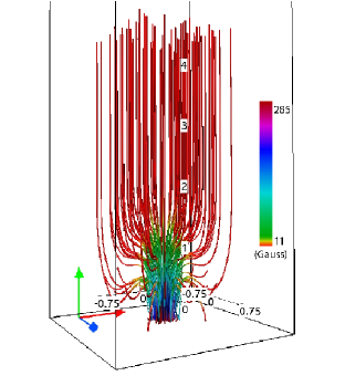
Figure 2: Equilibrium magnetic field lines. Red, green, and blue arrows correspond to the $x$-, $y$-, and $z$-axis, respectively. The size of the box shown is $(-0.75,0.75)\times(0,4)\times(-0.75,0.75)$ Mm. The color map corresponds to the magnitude of a magnetic field.

Figure 3: Equilibrium profiles of the Alfvén (solid) and sound (dashed) speeds (the left panel) and plasma $\beta$ (the right panel) along the flux tube axis.

2 A model of a solar magnetic flux tube of axial symmetry

We consider a model solar atmosphere that is described by the following ideal, adiabatic, 3D magnetohydrodynamic (MHD) equations:

$${{\partial\varrho}\over{\partial t}}+\nabla\cdot(\varrho{\bf V})=0\,,$$ (1)

$$\varrho{{\partial{\bf V}}\over{\partial t}}+\varrho\left({\bf V}\cdot\nabla\right){\bf V}=-\nabla p+\frac{1}{\mu}(\nabla\times{\bf B})\times{\bf B}+\varrho{\bf g}\,,$$ (2)

$${\partial p\over\partial t}+\nabla\cdot(p{\bf V})=(1-\gamma)p\nabla\cdot{\bf V}\,,\hskip 8.53581ptp=\frac{k_{\rm B}}{m}\varrho T\,,$$ (3)

$${{\partial{\bf B}}\over{\partial t}}=\nabla\times({\bf V}\times{\bf B})\,,\hskip 8.53581pt\nabla\cdot{\bf B}=0\ ,$$ (4)

where ${\varrho}$ is mass density, ${\bf V}$ is the flow velocity, and ${\bf B}$ is the magnetic field. The standard notation is used for the other physical parameters, namely, $p$, $T$, $\gamma=5/3$, $\mu$, ${\bf g}=(0,-g,0)$, $m$, and $k_{\rm B}$ are the gas pressure, temperature, adiabatic index, magnetic permeability, mean particle mass, and Boltzmann’s constant, respectively. The magnitude of the gravitational acceleration is $g=274$ m s^-2. The value of $m$ is specified by the mean molecular weight, which is $1.24$ in the solar photosphere (Oskar Steiner, private communication) and assumed to be constant in the entire flux tube model.

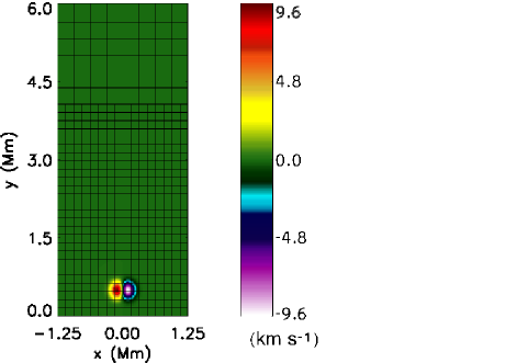
Figure 4: Numerical blocks with their boundaries (solid lines) and the pulse in velocity $V_{\rm z}$ of Eq. (30) (color maps) in the $x-y$ plane for $z=0$ Mm at $t=0$ seconds. A part of the simulation region is only displayed.

We assume that the solar atmosphere is in static equilibrium (${\bf V}_{\rm e}={\bf 0}$) with the Lorentz force balanced by the gravity force and the gas pressure gradient, which means that

$$\frac{1}{\mu}(\nabla\times{\bf B}_{\rm e})\times{\bf B}_{\rm e}+\varrho_{\rm e}{\bf g}-\nabla p_{\rm e}={\bf 0}\ ,$$ (5)

where the subscript ${}^{\prime}{\rm e}^{\prime}$ corresponds to the equilibrium configuration. We consider an axisymmetric flux tube whose equilibrium is described by Eq. (5) and its magnetic field satisfies the solenoidal condition. We now introduce the magnetic flux ($\Psi$) normalized by 2$\pi$, and obtain

$$\Psi(r,y)=\int_{0}^{r}B_{\rm ey}r^{\prime}\,dr^{\prime}\,,$$ (6)

where $B_{\rm ey}$ is a vertical magnetic field component and $r$ is the radial distance from the flux tube axis given by

$$r=\sqrt{x^{2}+z^{2}}\,.$$ (7)

As a result of Eq. (6), the magnetic field is automatically divergence-free and its radial ($B_{\rm er}$), azimuthal ($B_{\rm e\theta}$) and vertical ($B_{\rm ey}$) components are expressed as

$$B_{\rm er}=-\frac{1}{r}\frac{\partial\Psi}{\partial y}\,,\hskip 8.53581ptB_{\rm e\theta}=0\,,\hskip 8.53581ptB_{\rm ey}=\frac{1}{r}\frac{\partial\Psi}{\partial r}\,.$$ (8)

We consider a magnetic flux tube of axial symmetry, which is initially non-twisted, and represent the tube magnetic field in terms of its azimuthal component of the vector-potential ($A{\bf\hat{\theta}}$) as

$${\bf B_{\rm e}}=\nabla\times A{\bf\hat{\theta}}\,,$$ (9)

where ${\bf\hat{\theta}}$ is a unit vector along the azimuthal direction. In this case, we have

$$B_{\rm er}=-\frac{\partial A}{\partial y}\,,\hskip 8.53581ptB_{\rm e\theta}=0\,,\hskip 8.53581ptB_{\rm ey}=\frac{1}{r}\frac{\partial(rA)}{\partial r}\,.$$ (10)

Comparing Eqs. (8) and (10), we find

$$A(r,y)=\frac{1}{r}\Psi(r,y)\,.$$ (11)

In Cartesian coordinates the magnetic vector potential components are

$$[A_{\rm x},A_{\rm y},A_{\rm z}]=[A\frac{z}{r},0,-A\frac{x}{r}]\,.$$ (12)

These formulae are useful for numerical simulations because they identically satisfy the selenoidal condition, which is important in controlling numerical errors.

Multiplying now Eq. (5) by ${\bf B_{\rm e}}$, we obtain

$${\bf B_{\rm e}}\cdot(\nabla p_{\rm e}-\varrho_{\rm e}{\bf g})=0\,.$$ (13)

Since $p_{\rm e}=p_{\rm e}(\Psi,y)$, therefore, from the above equation with the use of Eq. (8), we have

$$\varrho_{\rm e}g=-\frac{\partial p_{\rm e}(\Psi,y)}{\partial y}\,,$$ (14)

which means that the hydrostatic condition is satisfied along magnetic field lines, and that $\Psi$ = const.

Rewriting Eq. (5) in its components and taking Eq. (8) into account, we obtain the so-called Grad-Shafranov equation (e.g., Low 1975; Priest 1982) given by

$$\frac{\partial^{2}\Psi}{\partial r^{2}}-\frac{1}{r}\frac{\partial\Psi}{\partial r}+\frac{\partial^{2}\Psi}{\partial y^{2}}=-\mu r^{2}\frac{\partial p_{\rm e}(\Psi,y)}{\partial\Psi}\,.$$ (15)

If we consider the equilibrium gas pressure as a given function, then Eq. (15) becomes a nonlinear Dirichlet problem for $\Psi$. In contrast, Low (1980) proposed the inverse problem by specifying magnetic field through a choice of $\Psi$ by integrating Eq. (15) and deriving the general formulas for $p_{\rm e}$ and $\varrho_{\rm e}$ given in terms of $\Psi$ and its derivatives. In our approach, we regard $y$ as a parameter, and after integrating Eq. (15) over $\Psi$, we find (Solov’ev 2010)

$$p_{\rm e}(r,y)=p_{\rm h}(y)-\frac{1}{\mu}\left[\frac{1}{2r^{2}}\left(\frac{\partial\Psi}{\partial r}\right)^{2}+\int\frac{\partial^{2}\Psi}{\partial y^{2}}\frac{\partial\Psi}{\partial r}\frac{dr}{r^{2}}\right]\,,$$ (16)

where

$$p_{\rm h}(y)=p_{\rm 0}\leavevmode\nobreak\ {\rm exp}\left[-\int_{y_{\rm r}}^{y}\frac{dy^{{}^{\prime}}}{\Lambda(y^{{}^{\prime}})}\right]\,,$$ (17)

is the hydrostatic gas pressure, and

$$\Lambda(y)=\frac{k_{\rm B}T_{\rm h}(y)}{mg}$$ (18)

is the pressure scale-height and $T_{\rm h}(y)$ is a hydrostatic temperature profile.

We adopt $T_{\rm h}(y)$ for the solar atmosphere that is specified by the model developed by Avrett & Loeser (2008). This temperature profile is smoothly extended into the corona (Fig. 1). It should be noted that in our model the solar photosphere occupies the region $0<y<0.5$ Mm, the chromosphere is sandwiched between $y=0.5$ Mm and the transition region, which is located at $y\simeq 2.1$ Mm, and that above this height the atmospheric layers represent the solar corona.

According to Eq. (14), the equilibrium mass density can be calculated if ${\partial p_{\rm e}(y,\Psi)}/{\partial y}$ is known. Moreover, from Eq. (16), we get $p_{\rm e}=p_{\rm e}(r,y)$. Thus, in order to find ${\partial p_{\rm e}(y,\Psi)}/{\partial y}$, we use the following relations that are valid for any differentiable function ($S$):

$$\frac{\partial S(r,y)}{\partial r} = \frac{\partial S(\Psi,y)}{\partial\Psi}\frac{\partial\Psi}{\partial r}\,,$$ (19)

$$\frac{\partial S(r,y)}{\partial y} = \frac{\partial S(\Psi,y)}{\partial y}+\frac{\partial S(\Psi,y)}{\partial\Psi}\frac{\partial\Psi}{\partial y}\,.$$ (20)

However, it follows from Eq. (16) that we need to specify $S(r,y)$ as

$$S(r,y)=\frac{1}{2r^{2}}\left(\frac{\partial\Psi}{\partial r}\right)^{2}+\int\frac{\partial^{2}\Psi}{\partial y^{2}}\frac{\partial\Psi}{\partial r}\frac{dr}{r^{2}}\,.$$ (21)

We calculate first ${\partial S(r,y)}/{\partial r}$, and then use Eq. (19) to determine ${\partial S(y,\Psi)}/{\partial\Psi}$. The result is

$$\frac{\partial p_{\rm e}(y,\Psi)}{\partial\Psi}=-\frac{1}{\mu}\left[\frac{1}{r}\frac{\partial}{\partial r}\left(\frac{1}{r}\frac{\partial\Psi}{\partial r}\right)+\frac{1}{r^{2}}\frac{\partial^{2}\Psi}{\partial y^{2}}\right]\,.$$ (22)

Using Eq. (20), we get

$$\frac{\partial p_{\rm e}(y,\Psi)}{\partial y}=\frac{\partial p_{\rm e}(r,y)}{\partial y}-\frac{\partial p_{\rm e}(y,\Psi)}{\partial\Psi}\frac{\partial\Psi}{\partial y}\,.$$ (23)

Finally, with help of Eq. (22), we write

$$\varrho_{\rm e}(r,y)=\varrho_{\rm h}(y)+$$

$$\frac{1}{\mu g}\{\frac{\partial}{\partial y}\left[\frac{1}{2r^{2}}\left(\left(\frac{\partial\Psi}{\partial r}\right)^{2}-\left(\frac{\partial\Psi}{\partial y}\right)^{2}\right)+\int\frac{\partial^{2}\Psi}{\partial y^{2}}\frac{\partial\Psi}{\partial r}\frac{dr}{r^{2}}\right]$$

$$-\frac{1}{r}\frac{\partial\Psi}{\partial y}\frac{\partial}{\partial r}\left(\frac{1}{r}\frac{\partial\Psi}{\partial r}\right)\}\,,$$ (24)

with

$$\varrho_{\rm h}(y)=\frac{p_{\rm h}(y)}{g\Lambda(y)}\,$$ (25)

being the hydrostatic mass density.

Note that in the above formulas the magnetic flux ($\Psi$) and consequently the magnetic flux function ($A$) are free to choose. For a flux tube, we can specify them as

$$A(r,y)=B_{\rm 0}\exp{(-k_{\rm y}^{2}y^{2})}\frac{r}{1+k_{\rm r}^{4}r^{4}}+\frac{1}{2}B_{\rm y0}r\,,$$ (26)

$$\Psi(r,y)=rA(r,y)\,,$$ (27)

where $B_{\rm y0}$ is the external magnetic field along the vertical direction, $k_{\rm r}$ and $k_{\rm y}$ are inverse length scales along the radial and vertical directions, respectively. The magnetic field lines, which follow from Eqs. (10) and (26) are displayed in Fig. 2 for $k_{\rm r}=k_{\rm y}=4$ Mm^-1. We choose the magnitude of the reference magnetic field $B_{\rm 0}$ in such way that the magnetic field within the flux tube, at $(x=0,y=0.5,z=0)$ Mm, is about $285$ Gauss, and $B_{\rm y0}\approx 11.4$ Gauss. For these values, the resulting magnetic field lines are predominantly vertical around the line, $x=z=0$ Mm, while further out they are bent and ${\bf B}_{\rm e}$ decays with distance from this line. It must be also noted that the magnetic field at the top of the simulation region is essentially uniform, with its value of $B_{\rm y0}$.

Figure 3 illustrates the sound speed, $c_{\rm s}$, (the dashed line in the left panel), Alfvén speed, $c_{\rm A}$, (the solid line in the same panel), and plasma $\beta$ (in the right panel) given by

$$c_{\rm s}(r,y)=\sqrt{\frac{\gamma p_{\rm e}(r,y)}{\varrho_{\rm e}(r,y)}}\,,\hskip 8.53581ptc_{\rm A}(r,y)=\sqrt{\frac{B_{\rm e}^{2}(r,y)}{\mu\varrho_{\rm e}(r,y)}}\,,$$ (28)

$$\beta(r,y)=\frac{2\mu p_{\rm e}(r,y)}{B_{\rm e}^{2}(r,y)}\,.$$ (29)

The sound speed below the transition region is smaller than $10$ km s^-1, however, it abruptly raises in the solar transition region, and then reaches its coronal value of 100 km s^-1 at the height $y=10$ Mm (not shown in the figure). The Alfvén speed reveals similar trends, reaching a value of more than $700$ km s^-1 at $y=10$ Mm (also not shown). The coronal plasma $\beta$ is $\approx 3\times 10^{-2}$ at $y=4$ Mm (the right panel). It increases with the depth but remains lower than $1$ above the height $y\approx 0.8$ Mm. It should be noted that as a result of strong magnetic field, $\beta$ is lower within the flux tube than in the surrounding medium (not shown).

3 Results of numerical simulations

Equations (1)-(4) are solved numerically using the code FLASH (Lee & Deane 2009; Lee 2013). This code implements a third-order unsplit Godunov solver (Murawski & Lee 2011) with various slope limiters and Riemann solvers, as well as adaptive mesh refinement. We choose the van Leer slope limiter and the Roe Riemann solver (Murawski & Lee 2012). For all the considered cases, we set the simulation box as $(-1.25,1.25)\,{\rm Mm}\times(0,20)\times(-1.25,1.25)\,{\rm Mm}$, and impose boundary conditions by fixing in time all plasma quantities at all six boundary surfaces to their equilibrium values. In the present numerical studies, we use a non-uniform grid with a minimum (maximum) level of refinement set to $2$ ($5$). The grid system at $t=0$ s is shown in Fig. 4 with the blocks being displayed only up to $y=6$ Mm. Above this altitude the block system remains homogeneous. As each block consists of $8\times 8\times 8$ identical numerical cells, we reach the effective finest spatial resolution of $19.53$ km, below the altitude $y=4.25$ Mm.

We initially perturb the azimuthal component of velocity, $V_{\theta}$, by using

$$V_{\theta}{\bf\hat{\theta}}=[V_{\rm x},V_{\rm z}]=[\frac{z}{w},-\frac{x}{w}]\ A_{\rm v}\exp\left[-\frac{r^{2}+(y-y_{\rm 0})^{2}}{w^{2}}\right],$$ (30)

where $A_{\rm v}$ denotes the amplitude of the pulse, ${\bf\hat{\theta}}$ is the unit vector along the azimuthal direction, $y_{\rm 0}$ is its vertical position, and $w$ is the width. We set $A_{\rm v}=150$ km s^-1, $w=150$ km, and $y_{\rm 0}=500$ km, and hold them fixed. This value of $A_{\rm v}$ results in the effective maximum velocity of about $9.6$ km s^-1 (Fig. 4).

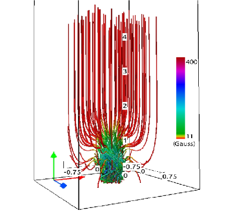
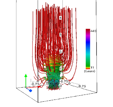
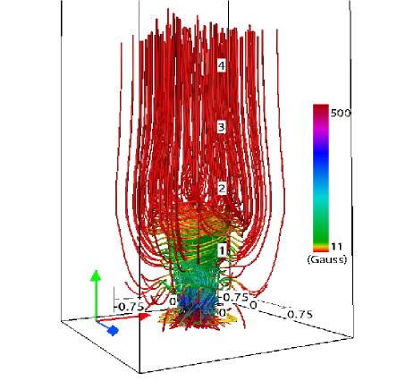
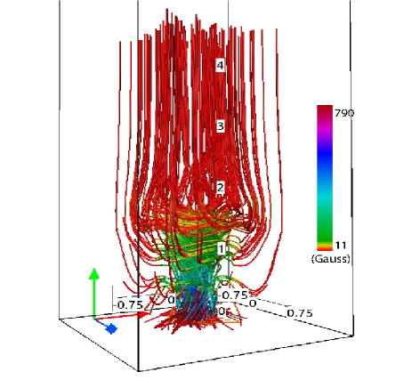
Figure 5: Magnetic field lines at $t=50$ s (top-left), $t=150$ s (top-right), $t=200$ s (bottom-left), and $t=250$ s (bottom-right). Red, green and blue arrows design the directions of the $x$-, $y$-, and $z$-axis, respectively. The size of the box shown is $(-0.75,0.75)\times(0,4)\times(-0.75,0.75)$ Mm. The color map corresponds to the magnitude of a magnetic field.

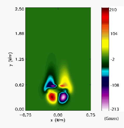
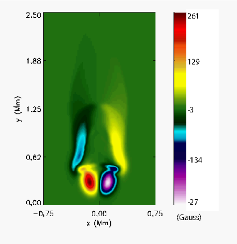
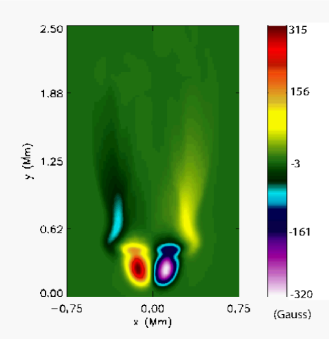
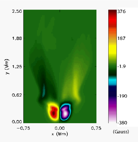
Figure 6: Spatial profiles of $B_{\rm z}(x,y,z=0)$ associated with torsional Alfvén waves, at $t=50$ s (top-left), $t=100$ s (top-right), $t=150$ s (bottom-left), and $t=200$ s (bottom-right). A part of the simulation region is displayed only.

The initial velocity pulse of Eq. (30) triggers torsional Alfvén waves. These waves are illustrated in Fig. 5, which shows magnetic field lines at $t=50$ s (the top-left panel), $t=150$ s (the top-right panel), $t=200$ s (the bottom-left panel), and $t=250$ s (the bottom-right panel). At $t=50$ s (the top-left panel) the upwardly propagating Alfvén waves, while observed in $B_{\theta}$, reach the altitude $y\approx 1$ Mm, and at a later time Alfvén waves spread in space while propagating along diverged magnetic field lines (the top-right and bottom panels).

Note that small-amplitude magnetic field and velocity perturbations that include the effect of magnetic field expansion, are governed by the following wave equations (Eqs. (3) & (4) in Hollweg 1981):

$$\frac{\partial^{2}\left(r^{2}v\right)}{\partial t^{2}}=\frac{B_{\rm e}}{\mu\varrho_{\rm e}}\frac{\partial}{\partial s}\left[r^{2}B_{e}\frac{\partial v}{\partial s}\right]\,,$$ (31)

$$\frac{\partial^{2}b}{\partial t^{2}}=r^{2}B_{\rm e}\frac{\partial}{\partial s}\left(\frac{B_{\rm e}}{\mu\varrho_{\rm e}r^{2}}\frac{\partial b}{\partial s}\right)\,,$$ (32)

where $v=V_{\theta}/r$, $b=rB_{\theta}$, $V_{\theta}$ and $B_{\theta}$ are the azimuthal components of respectively perturbed velocity and magnetic field, and $s$ is the coordinate along the magnetic field lines.

Moran (2001) showed that $V_{\theta}\propto\varrho_{\rm e}^{-1/4}/AB_{\rm e}$, where $A$ is the cross-sectional area of the flux tube. Near the flux tube axis we can take $AB_{\rm e}$ approximately constant, hence in that region $V_{\theta}\propto\varrho_{\rm e}^{-1/4}$. On the other hand, $B_{\theta}\propto\varrho_{\rm e}^{1/4}$ (Moran 2001). Hence, near the flux tube axis, these quantities are only dependent on the variation of $\varrho_{\rm e}$, with $V_{\theta}$ and $B_{\theta}$ respectively growing and decreasing with height. As a result of that the perturbations of magnetic field lines remain weak in the solar corona (see also Murawski & Musielak 2010 for the corresponding analysis in the case of the straight vertical magnetic field lines).

Ratio of magnetic to kinetic energies (evaluated in the entire computational domain) of Alfvén waves is shown in Fig. 7 (top). Initially, at $t=0$ s, as we launch the initial pulse in the azimuthal velocity alone the magnetic energy is zero at $t=0$ s but, according to our numerical simulations, contributions of the magnetic energy grow in time. It is well known that for torsional Alfvén waves, there is the equipartition between potential and kinetic energies. Hence according to the top panel of Fig. 7, this equipartition of energy is not reached in the numerical simulation until about $t=200$ s (where the energy ratio equals unity). This is the natural explanation for the limiting value of the energy ratio being approximately unity at $t=200$ s. At $t=225$ s the magnetic energy is higher than the kinetic energy with the ratio equal to $\approx 1.1$. Ratios of slow magnetoacoustic waves energy to Alfvén waves energy (asterisks) and fast magnetoacoustic waves energy to Alfvén waves energy (diamonds) is illustrated in Fig. 7 (bottom). At $t=0$ s kinetic energies of both the slow and fast magnetoacoustic waves are zero but as these waves are driven by the ponderomotive force which results from Alfvén waves the energy ratio grows in time reaching a maximum level of about $0.25$ which means that about $25\%$ of the Alfvén wave energy was converted into kinetic energies of magnetoacoustic waves. These waves propagate along magnetic field lines and power the vertical plasma flows in form of the jets.

Figure 7: The top panel: ratio of magnetic to kinetic energies of Alfvén waves; the bottom panel: ratio of slow magnetoacoustic waves kinetic energy to Alfvén waves energy (asterisks) and ratio of fast magnetoacoustic waves kinetic energy to total energy of Alfvén waves (diamonds). These energies are evaluated by integration in space over the entire computational domain.

Figure 8: Maximum of $V_{\theta}$ (left-panel) and $B_{\theta}$ (right-panel) vs height. The numerical (analytical) data points are represented by asterisks (solid line).

Figure 8 illustrates maximum of $V_{\theta}$ (left-panel) and $B_{\theta}$ (right-panel) as evaluated from the numerical data. We clearly see that $V_{\theta}$ grows with height as predicted on the basis of the liner theory approximation reported by Moran (2001). On the other hand, $B_{\theta}$ exhibits a fall-off with $y$ with the numerical data points being close to the linear theory data (solid-line) as reported by Moran (2001). It must also be noted that the relationships shown by Moran (2001) are only valid when there is the equipartition of energy for torsional Alfvén waves. According to the top panel of Fig. 7, this occurs only the time of our numerical simulations is $t=200$ s or longer. As the results of Fig. 8 are given for the times shorter than $t=200$ s, then comparison of these results with the analytical findings of Moran (2001) is not strictly valid. This fall-off is also clearly evident in the spatial profiles of $B_{\rm z}(x,y,z=0)$ as displayed at $t=150$ s and $t=200$ s (Fig. 6, bottom panels). At $t=50$ s and $t=100$ s (top panels), the perturbations of $B_{\rm z}(x,y,z=0)$ are localized below the transition region but at later times the perturbations that penetrate the inner solar corona are of significantly lower magnitude than those remaining below the transition region. Consequently, these profiles demonstrate clearly that Alfvén waves, while traced in perturbed magnetic field lines, are essentially located below the transition region, which agrees with the conclusions of Murawski & Musielak (2010) who used the analytical and numerical techniques for the 1D wave equations and found that magnetic field perturbations, while excited below the transition region, remain week in the solar corona in comparison to the perturbations in lower atmospheric layers.

Figure 9 shows temporal snapshots of velocity streamlines at $t=100$ s (the left-top panel), $t=150$ s (the right-top panel), $t=200$ s (the left-bottom panel), and $t=225$ s (the right-bottom panel). These streamlines are defined by the following equations:

$$\frac{dx}{V_{\rm x}}=\frac{dy}{V_{\rm y}}=\frac{dz}{V_{\rm z}}\,.$$ (33)

Note that a signal in the azimuthal velocity is clearly seen in the solar corona. Indeed, the streamlines show that velocity perturbations penetrate the transition region and enter the solar corona, leading to a generation of the main centrally located vortex, which starts developing at $t=100$ s.

Our results clearly show that the velocity perturbations are significantly enhanced in the solar transition region as a result of very steep temperature gradient. The main physical consequence of this decrease is that in the inner corona, just above the transition region, we see the more velocity streamline perturbations (Figs. 9), while we do not see much perturbations of the azimuthal component of the magnetic fields (cf., Figs. 5-6). Note that in the linear limit, $V_{\theta}$ is governed by the wave equation of Eq. (31) which was derived by Hollweg (1981). This equation differs from Eq. (32), and this difference affects the evolution scenario of velocity perturbations.

Torsional Alfvén waves can be traced in the vertical profiles of $V_{\rm z}(x,y,z=0)=V_{\theta}(x,y,z=0)$ (see Fig. 10). At $t=200$ s (the bottom-right panel), the upwardly propagating Alfvén waves resulting from the initial pulse are well seen, with their amplitudes of $|V_{\rm z}|\approx 16$ km s^-1. The downwardly propagating waves subside as it is discernible at $t=100$ s (the top-right panel) and at $t=150$ s (the bottom-left panel). At $t=100$ s, the upwardly propagating waves reach the altitude of more than $y=1.6$ Mm as shown in the top-right panel of the figure.

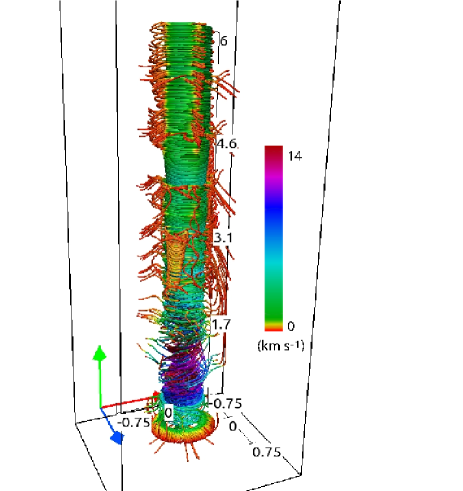
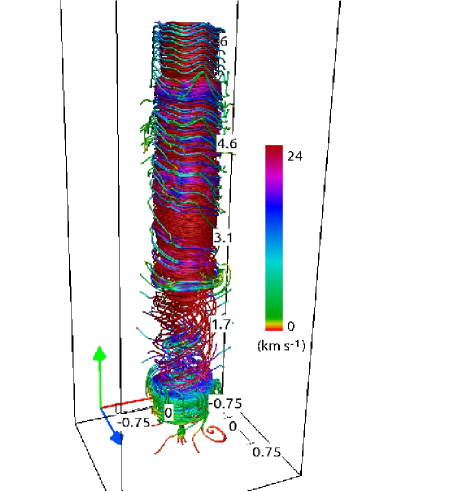
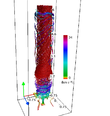
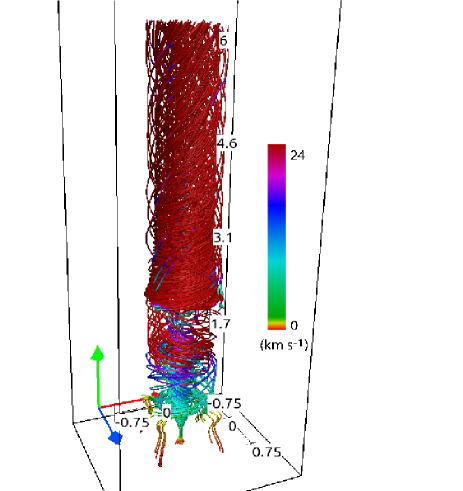
Figure 9: Streamlines at $t=100$ s (top-left), $t=150$ s (top-right), $t=200$ s (bottom-left), and $t=225$ s (bottom-right). Red, green and blue arrows design the directions of the $x$-, $y$-, and $z$-axis, respectively. The size of the box shown is $(-0.75,0.75)\times(0,6)\times(-0.75,0.75)$ Mm. The color map corresponds to the magnitude of a total velocity.

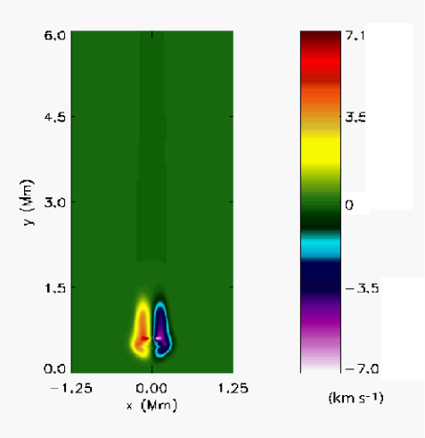
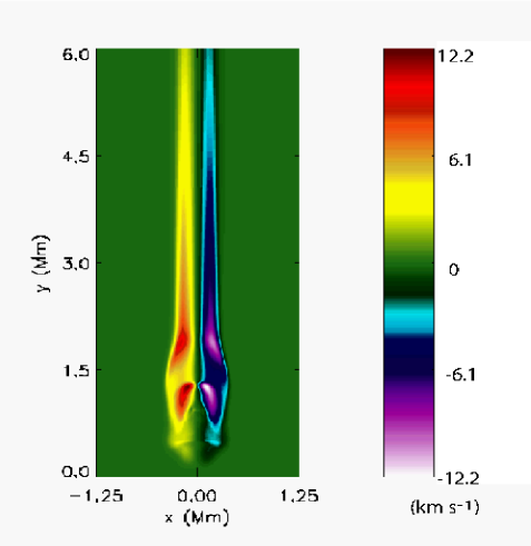
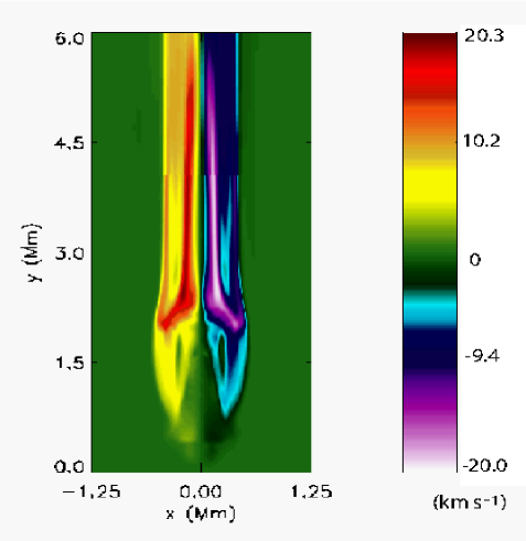
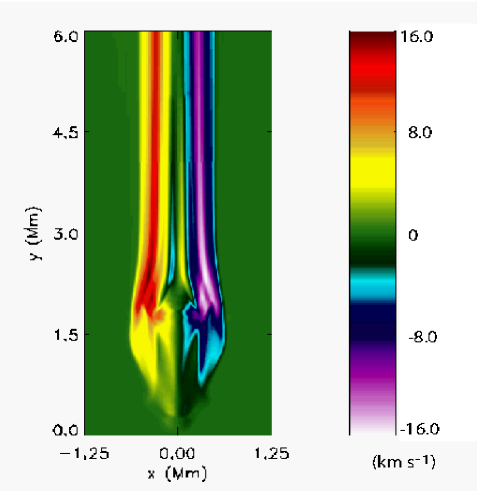
Figure 10: Spatial profiles of $V_{\rm z}(x,y,z=0)$ associated with torsional Alfvén waves at $t=50$ s (the top-left panel), $t=100$ s (the top-right panel), $t=150$ s (the bottom-left panel) and $t=200$ s (the bottom-right panel).

As a result of nonlinearity, torsional Alfvén waves drive a vertical flow through a ponderomotive force (Hollweg et al. 1982; Nakariakov et al. 1997, 1998). We refer to Eq. (6) in Hollweg et al. (1982) which illustrates all the terms which contribute to the component of velocity that is parallel to a magnetic field line, $V_{\parallel}$. Denoting by $s$ distance measured along this line and by $r(s)$ a distance of any point on this line from the $y$-axis we restate Eq. (6) in Hollweg et al. (1982) as

$$\frac{\partial}{\partial t}\left(\frac{\varrho V_{\parallel}}{B_{\parallel}}\right)+\frac{\partial}{\partial s}\left(\frac{\varrho V_{\parallel}^{2}}{B_{\parallel}}\right)=-\frac{1}{B_{\parallel}}\frac{\partial p}{\partial s}+\frac{\varrho g_{\parallel}}{B_{\parallel}}+$$

$$\frac{1}{B_{\parallel}}\left[\left(\varrho V_{\theta}^{2}-\frac{1}{\mu}B_{\theta}^{2}\right)\frac{\partial\,\ln r}{\partial s}-\frac{\partial}{\partial s}\left(\frac{B_{\theta}^{2}}{2\mu}\right)\right]\,,$$ (34)

where $g_{\parallel}$ and $B_{\parallel}$ are the components of, respectively, the gravitational acceleration and perturbed magnetic field along the magnetic field line, and $V_{\theta}$ and $B_{\theta}$ are azimuthal components of velocity and magnetic field, respectively. Following Hollweg et al. (1982), we state that the terms in the square bracket result from the $s$-component of the Lorentz force: the first term denotes the $s$-component of the centrifugal force that corresponds to twisting motions; the second term represents the magnetic tension; the third term is the magnetic pressure.

The vertical flow can be seen in the spatial profiles of $V_{\rm y}(x,y,z=0)$ (Fig. 11, middle). At $t=400$ s, slow magnetoacoustic waves in a low plasma $\beta$ region of the magnetic flux tube of axial symmetry as displayed in the right-panel of Fig. 3 are weakly coupled to fast magnetoacoustic waves, which are described by essentially only $V_{\rm y}$ component of the velocity. Our simulations demonstrate that at $t=175$ s slow magnetoacoustic waves already penetrated the solar corona, reaching the level higher than $y=4.5$ Mm.

It is noteworthy that non-linear torsional Alfvén waves drive perturbations in a mass density, which are associated with fast (Fig.  11, top) and predominantly slow (Fig.  11, middle) magnetoacoustic waves. The vertical spatial profile of $\log(\varrho(x,y,z=0)/\varrho_{\rm 0})$ is shown at $t=225$ s in the bottom panel of Fig. 11. Here $\varrho_{\rm 0}=10^{-12}$ kg m^-3 is the hydrostatic mass density at the level $y=10$ Mm. At this time the dense plasma jets reach the altitude of $y\approx 3.5$ Mm. The plasma is lifted up due to the magnetic pressure gradient originating from the Alfvén waves and acts against the gravity to push the chromospheric material up to the inner solar corona. Therefore, such predominant vertical pressure can create the cool plasma jet flows typically observed in the solar corona.

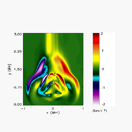
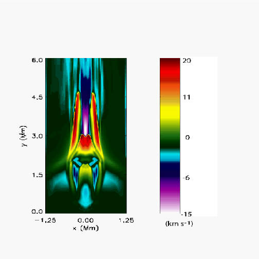
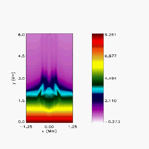
Figure 11: Spatial profiles of $V_{\rm x}(x,y,z=0)$ at $t=100$ s (top), $V_{\rm y}(x,y,z=0)$ at $t=175$ s (middle) and $\log(\varrho(x,y,z=0)/\varrho_{\rm 0})$ at $t=225$ s (bottom), where $\varrho_{\rm 0}=10^{-12}$ kg m^-3 is the hydrostatic mass density at the level $y=10$ Mm.

Figure 12: Time-signatures of velocities $V_{\rm z}$ (solid line) and $V_{\rm y}$ (dashed line), collected just below the transition region at the detection point $(x=0.1,y=1.9,z=0.1)$ Mm.

Figure 12 displays the time-signatures of $V_{\rm z}$ (the solid line) and $V_{\rm y}$ (the dashed line) collected at the detection point, $(x=0.2,y=3.5,z=0.2)$ Mm. We infer that slow magnetoacoustic waves, represented by $V_{\rm y}$, reach the detection point at $t\approx 130$ s, while Alfvén waves arrive at this point about $30$ s earlier.

Noting that up to $y\approx 0.7$ Mm Alfvén speed is lower than the sound speed (Fig. 3, left), the travel times of the torsional Alfvén, $t_{\rm At}(y)$, and slow magnetoacoustic waves, $t_{\rm st}(y)$, are given by

$$t_{\rm At}(y)\approx\int_{0.5}^{y}\frac{d{\tilde{y}}}{c_{\rm A}(r,{\tilde{y}})}\,,$$ (35)

$$t_{\rm st}(y)\approx\int_{0.5}^{y}\frac{d{\tilde{y}}}{c_{\rm T}(r,{\tilde{y}})}\,,$$ (36)

where the integration is performed along the corresponding magnetic field line, and $c_{\rm T}=c_{\rm s}c_{\rm A}/\sqrt{c_{\rm s}^{2}+c_{\rm A}^{2}}$ is the tube speed. Using Eqs. (35) and (36), we find $t_{\rm At}(y=1.9)\approx 157.7$ s and $t_{\rm st}(y=1.9)\approx 173.3$ s. These values are larger than the arrival times of Alfvén and slow magnetoacoustic waves. This dispatch results from nonlinearity.

The amplitude of the Alfvén waves, seen in $V_{\theta}$, penetrating into the upper region of the atmosphere drops from about $V_{\theta}=9$ km s^-1 at $t=100$ s just under the transition region, through $V_{\theta}=8.4$ km s^-1 just above the transition region. We can evaluate the transmission coefficient,

$$C_{\rm t}=\frac{A_{\rm t}}{A_{\rm i}}\,,$$ (37)

where $A_{\rm i}$ ($A_{\rm t}$) is the amplitude of the incident (transmitted) waves. Substituting $A_{\rm i}=9$ km s^-1 and $A_{\rm t}=8.4$ km s^-1 into the above formula we get $C_{\rm t}\approx 0.95$, which means that about than $5$% of the waves amplitude became reflected in the transition region and about $95$% was transmitted into upper atmospheric layers. These are rough estimates due to difficulties with precise estimation of wave amplitudes which highly vary in time at the transition region.

4 Discussion and Conclusions

In this paper, we present an analytical model of a magnetic flux tube of axial symmetry embedded in the solar atmosphere whose photosphere, chromosphere and transition region are described by the model of Avrett & Loeser (2008). Our flux tube model can easily be adopted to any axisymmetric magnetic structure by specifying a different magnetic flux. The model was used to perform numerical simulations of the propagation of torsional Alfvén waves and their coupling to magnetoacoustic waves by using the FLASH code. Torsional Alfvén waves are launched at the top of the solar photosphere by an initial localized pulse in the azimuthal component of velocity. This pulse mimics the convectively excited photospheric vortices or any other kind of plasma rotatory motions recently observed in the solar atmosphere (see Section 1 for references and discussion).

Our results show a complex behavior of torsional Alfvén waves and the driven magnetoacoustic waves, and their responses in the solar chromosphere, transition region, and inner corona. The time and spatial evolution of Alfvén waves shown by our numerical results is akin to the dynamics of fast solar swirling motions observed in the form of various jets at diverse spatio-temporal scales. Therefore, our model presented here has a potential to describe the physics of various observed and recurring swirling motions (jets) in the solar atmosphere in which the driver excites torsional Alfvén waves as well as the associated plasma perturbations (e.g., Wedemeyer-Böhm et al. 2012; Murawski et al. 2014, and references cited therein).

Since in our model the solar magnetic flux tube of axial symmetry is strongly magnetized in the solar photosphere, it can be either associated with strong magnetic bright points (MBPs) (Jess et al. 2009) or with the concentration of the magnetic field between intergranular lanes (Wedemeyer-Böhm et al. 2012). With the use of the Swedish Solar Telescope Jess et al. (2009) observed the periodic variations above such MBPs in the detected (at different altitudes) Doppler widths of the H_α line. The authors claimed that their findings reveal the presence of the propagating torsional Alfvén waves with their wave periods of $2-12$ min up to the top of the solar chromosphere in the expanding wave-guide rooted in the strongly magnetized MBP. Clearly, our developed model can be used to excite torsional Alfvén waves and comparing the theoretically predicted range of wave frequencies to that established observationally. Indeed, this was one of the main goals achieved in our paper and we found the theoretical wave periods to be smaller than $100$ s (Fig. 12), which are close to the observational findings of Jess at al. (2009).

Our numerical results also show that the excited perturbations in azimuthal component of the magnetic field (Fig. 6) are seen below the solar transition region. However, in the inner corona these perturbations are of a significantly lower amplitude. On the other hand, the perturbations in azimuthal component of velocity are stronger in the solar corona.

Finally, let us point out that our analytical model can easily be adopted to derive the equilibrium conditions for any axisymmetric 3D magnetic structure. Our devised numerical model of the solar magnetic flux tube of axial symmetry can be applicable to the variety of flux tubes with different photospheric fields, and different expansions, as well as with different strengths of the drivers. The model can also be used to investigate the nonlinear evolution of coupled torsional Alfvén and magnetoacoustic waves, and to determine and understand drivers of coronal jets.

Acknowledgments. We are indebted to the referee for his/her valuable comments and suggestions that allowed us to significantly improve the original version of our paper. K.M. expresses his gratitude to Zdzislaw Musielak for hospitality during his visit to the University of Texas at Arlington in Spring 2014, when a part of this project was done; the visit as well as the project described in this paper were supported by NSF under the grant AGS 1246074 (Z.E.M. & K.M.). The work has also been supported by a Marie Curie International Research Staff Exchange Scheme Fellowship within the 7th European Community Framework Program (K.M., A.S., & J.K.). In addition, A.S. thanks the Presidium of Russian Academy of Sciences for the support in the frame of Program 22 and Russian Foundation of Fundamental Researches under the Grant 13-02-00714. The software used in this work was in part developed by the DOE-supported ASCI/Alliance Center for Astrophysical Thermonuclear Flashes at the University of Chicago. The 2D and 3D visualizations of the simulation variables have been carried out using respectively the IDL (Interactive Data Language), Python, and VAPOR (Visualization and Analysis Platform) software packages.

References

- (1) Avrett E.H., Loeser R., 2008, ApJS, 175, 228
- (2) Bonet J.A., Marquez I., Sanchez Almeida J., Cabello I., Domingo V., 2008, ApJ, 687, 431
- (3) Cargill P., Spicer D.S., Zalesak L.S., 1997, ApJ, 488, 854
- (4) Chmielewski P., Srivastava A.K., Murawski K., Musielak Z.E., 2013, MNRAS, 428, 40
- (5) Chmielewski P., Murawski K., A. A. Solov’ev, 2014, Res. Astron. Astrophys., 14, 855
- (6) De Pontieu B., Carlsson M., Rouppe van der Voort L.H.M., Rutten R.J., Hansteen V.H., Watanabe H., 2012, ApJ, 752, L12
- (7) Dwivedi B.N., Srivastava A.K., 2006, Sol. Phys., 237, 143
- (8) Dwivedi B.N., Srivastava A.K., 2010, Current Science, 98, 295
- (9) Fedun V, Verth G., Jess D. B., Erdélyi, 2011, ApJ, 740, L46
- (10) Ferriz-Mas A., Schüssler M., Anton V., 1989, A&A, 210, 425
- (11) Fujimura D., Tsuneta S., 2009, ApJ, 702, 1443
- (12) Gent F.A., Fedun V., Mumford S.J., Erdélyi R., 2013, MNRAS, 435, 689
- (13) Gruszecki M., Murawski K., Ofman L., 2008, A&A, 488, 757
- (14) Heinemann M., Olbert S., 1980, JGR, 85, 1311
- (15) Hollweg J.V., 1978, Sol. Phys., 56, 305
- (16) Hollweg J.V., 1981, Sol. Phys., 70, 25
- (17) Hollweg J.V., Jackson S., Galloway D., 1982, Solar Phys., 75, 35
- (18) Hollweg J.V., 1992, ApJ, 389, 731
- (19) Jess D.B., Mathioudakis M., Erdélyi R., Crokett P.J., Keenan F.P., Christian D.J., 2009, Science, 323, 1582
- (20) Kudoh T., Shibata K., 1999, ApJ, 514, 493
- (21) Lee D., 2013, J. Comput. Phys., 243, 269
- (22) Lee D., Deane A.E., 2009, J. Comput. Phys., 228, 952
- (23) Low B.C., 1975, ApJ, 197, 251
- (24) Low B.C., 1980, Solar Phys., 67, 57
- (25) Moran T.G., 2001, A&A, 374, L9
- (26) Murawski K., Lee D., 2011, Bull. Pol. Ac.: Tech., 59, 81
- (27) Murawski K., Lee D., 2012, Control and Cybernetics, 41, 35
- (28) Murawski K., Musielak Z.E., 2010, A&A, 518, A37
- (29) Murawski K., Ballai I, Srivastava A.K., Lee D., 2013, MNRAS, 436, 1268
- (30) Murawski K., Srivastava A.K., Musielak Z.E., 2014, ApJ, 788, 8
- (31) Musielak, Z. E., 1998, Proceedings of the Third SOLTIP Symposium on Solar and Interplanetary Transient Phenomena, Beijing, China, Eds. X.S. Feng, F.S. Wei & M. Dryer, 339
- (32) Musielak Z.E, Moore R.J., 1995, ApJ, 452, 434
- (33) Musielak Z.E., Routh S., Hammer R., 2007, ApJ, 659, 650
- (34) Nakariakov V.M., Roberts B., Murawski K., 1997, Sol. Phys., 175, 93
- (35) Nakariakov V.M., Roberts B., Murawski K., 1998, A&A, 332, 795
- (36) Ofman L., 2009, Sp. Sci. Rev., 149, 153
- (37) Okamoto T.J., De Pontieu B., 2011, ApJL, 736, 6
- (38) Priest E.R., 1982, Solar Magnetohydrodynamics, Dordrecht-Reidel, London
- (39) Routh S., Musielak Z.E., Hammer R., 2007, Sol. Phys., 38, 894
- (40) Routh S., Musielak Z.E., Hammer R., 2010, ApJ, 709, 1297
- (41) Saito T., Kudoh T., Shibata K., 2001, ApJ, 554, 1151
- (42) Sekse D.H., Rouppe van der Voort L., De Pontieu B., Scullion E., 2013, ApJ, 769, 44
- (43) Shelyag S., Cally P.S., Reid A., Mathioudakis M., 2013, ApJL, 776, L4
- (44) Solov’ev A.A., 2010, Astronomy Reports, 54, 85
- (45) Ulmschneider P., Musielak Z.E., 1998, A&A, 338, 311
- (46) Ulmschneider, P., Musielak, Z.E. 2003, in 21st NSO/SP Workshop on Current Theoretical Models and Future High Resolution Solar Observations: Preparation for ATST, A.A. Pevtsov and H. Uitenbrock, Eds, ASP Conf. Ser., 286, 363
- (47) Van Doorsselaere T., Nakariakov V.M., Verwichte E., 2008, ApJ, 676, L73
- (48) Vasheghani Farahani S., Nakariakov V.M., van Doorsselaere T., Verwichte E., 2011, A&A, 526, A80
- (49) Vasheghani Farahani S., Nakariakov V.M., Verwichte E., Van Doorsselaere T., 2012, A&A, 544, A127
- (50) Vigeesh G., Fedun V., Hasan S.S., Erdélyi R., 2012, ApJ, 755, 11
- (51) Wedemeyer-Böhm S., van der Voort L.R., 2009, A&AL, 507, L9
- (52) Wedemeyer-Böhm S., Scullion, E., Steiner O., Rouppe van der Voort L., de La Cruz Rodriguez J., Fedun V., Erdélyi R., 2012, Nature, 486, 505
- (53) Zaqarashvili T.V., Murawski K., 2007, A&A, 470, 353