A Tutorial on Inverse Problems for Anomalous Diffusion Processes

Abstract.

Over the last two decades, anomalous diffusion processes in which the mean squares variance grows slower or faster than that in a Gaussian process have found many applications. At a macroscopic level, these processes are adequately described by fractional differential equations, which involves fractional derivatives in time or/and space. The fractional derivatives describe either history mechanism or long range interactions of particle motions at a microscopic level. The new physics can change dramatically the behavior of the forward problems. For example, the solution operator of the time fractional diffusion diffusion equation has only limited smoothing property, whereas the solution for the space fractional diffusion equation may contain weakly singularity. Naturally one expects that the new physics will impact related inverse problems in terms of uniqueness, stability, and degree of ill-posedness. The last aspect is especially important from a practical point of view, i.e., stably reconstructing the quantities of interest.

In this paper, we employ a formal analytic and numerical way, especially the two-parameter Mittag-Leffler function and singular value decomposition, to examine the degree of ill-posedness of several “classical” inverse problems for fractional differential equations involving a Djrbashian-Caputo fractional derivative in either time or space, which represent the fractional analogues of that for classical integral order differential equations. We discuss four inverse problems, i.e., backward fractional diffusion, sideways problem, inverse source problem and inverse potential problem for time fractional diffusion, and inverse Sturm-Liouville problem, Cauchy problem, backward fractional diffusion and sideways problem for space fractional diffusion. It is found that contrary to the wide belief, the influence of anomalous diffusion on the degree of ill-posedness is not definitive: it can either significantly improve or worsen the conditioning of related inverse problems, depending crucially on the specific type of given data and quantity of interest. Further, the study exhibits distinct new features of “fractional” inverse problems, and a partial list of surprising observations is given below.

• Classical backward diffusion is exponentially ill-posed, whereas time fractional backward diffusion is only mildly ill-posed in the sense of norms on the domain and range spaces. However, this does not imply that the latter always allows a more effective reconstruction.

• Theoretically, the time fractional sideways problem is severely ill-posed like its classical counterpart, but numerically can be nearly well-posed.

• The classical Sturm-Liouville problem requires two pieces of spectral data to uniquely determine a general potential, but in the fractional case, one single Dirichlet spectrum may suffice.

• The space fractional sideways problem can be far more or far less ill-posed than the classical counterpart, depending on the location of the lateral Cauchy data.

In many cases, the precise mechanism of these surprising observations is unclear, and awaits further analytical and numerical exploration, which requires new mathematical tools and ingenuities. Further, our findings indicate fractional diffusion inverse problems also provide an excellent case study in the differences between theoretical ill-conditioning involving domain and range norms and the numerical analysis of a finite-dimensional reconstruction procedure. Throughout we will also describe known analytical and numerical results in the literature.
Keywords: fractional inverse problem; fractional differential equation; anomalous diffusion; Djrbashian-Caputo fractional derivative; Mittag-Leffler function.

1. Introduction

Diffusion is one of the most prominent transport mechanisms found in nature. At a microscopic level, it is related to the random motion of individual particles, and the use of the Laplace operator and the first-order derivative in the canonical diffusion model rests on a Gaussian process assumption on the particle motion, after Albert Einstein’s groundbreaking work [23]. Over the last two decades a large body of literature has shown that anomalous diffusion models in which the mean square variance grows faster (superdiffusion) or slower (subdiffusion) than that in a Gaussian process under certain circumstances can offer a superior fit to experimental data (see the comprehensive reviews [72, 95, 5, 70] for physical background and practical applications). For example, anomalous diffusion is often observed in materials with memory, e.g., viscoelastic materials, and heterogeneous media, such as soil, heterogeneous aquifer, and underground fluid flow. At a microscopic level, the subdiffusion process can be described by a continuous time random walk [75], where the waiting time of particle jumps follows some heavy tailed distribution, whereas the superdiffusion process can be described by Lévy flights or Lévy walk, where the length of particle jumps follows some heavy tailed distribution, reflecting the long-range interactions among particles. Following the aforementioned micro-macro correspondence, the macroscopic counterpart of a continuous time random walk is a differential equation with a fractional derivative in time, and that for a Lévy flight is a differential equation with a fractional derivative in space. We will refer to these two cases as time fractional diffusion and space fractional diffusion, respectively, and it is generically called a fractional derivative equation (FDE) below. In general the fractional derivative can appear in both time and space variables.

Next we give the mathematical model. Let $\Omega=(0,1)$ be the unit interval. Then a general one-dimensional FDE is given by

(1.1) $$\partial_{t}^{\alpha}u-{\,{}_{0}^{C}\kern-1.99997ptD^{\beta}_{\kern-0.70004ptx}}u+qu=f\quad(x,t)\in\Omega\times(0,T),$$

where $T>0$ is a fixed time, and it is equipped with suitable boundary and initial conditions. The fractional orders $\alpha\in(0,1)$ and $\beta\in(1,2)$ are related to the parameters specifying the large-time behavior of the waiting-time distribution or long-range behavior of the particle jump distribution. For example, in hydrological studies, the parameter $\beta$ is used to characterize the heterogeneity of porous medium [17]. In theory, these parameters can be determined from the underlying stochastic model, but often in practice, they are determined from experimental data [34, 35, 61]. The notation $\partial_{t}^{\alpha}={\,{}_{0}^{C}\kern-1.99997ptD^{\alpha}_{\kern-0.70004ptt}}$ is the Djrbashian-Caputo derivative operator of order $\alpha\in(0,1)$ in the time variable $t$, and $\,{}_{0}^{C}\kern-1.99997ptD^{\beta}_{\kern-0.70004ptx}$ denotes the Djrbashian-Caputo derivative of order $\beta\in(1,2)$ in the space variable $x$. For a real number $n-1<\gamma<n$, $n\in\mathbb{N}$, and $f\in H^{n}(0,1)$, the left-sided Djrbashian-Caputo derivative $\,{}_{0}^{C}\kern-1.99997ptD^{\gamma}_{\kern-0.70004ptx}f$ of order $\gamma$ is defined by [53, pp. 91]

(1.2) $$\,_{0}^{C}\kern-1.99997ptD^{\gamma}_{\kern-0.70004ptx}f=\frac{1}{\Gamma(n-\gamma)}\int_{0}^{x}(x-s)^{n-1-\gamma}f^{(n)}(s)ds,$$

where $\Gamma(z)$ denotes Euler’s Gamma function defined by

$$\Gamma(z)=\int_{0}^{\infty}s^{z-1}e^{-s}ds,\quad\ \Re(z)>0.$$

The Djrbashian-Caputo derivative was first introduced by Armenian mathematician Mkhitar M. Djrbashian for studies on space of analytical functions and integral transforms in 1960s (see [21, 20, 19] for surveys on related works). Italian geophysicist Michele Caputo independently proposed the use of the derivative for modeling the dynamics of viscoelastic materials in 1967 [10]. We note that there are several alternative (and different) definitions of fractional derivatives, notably the Riemann-Liouville fractional derivative, which formally is obtained from (1.2) by interchanging the order of integration and differentiation, i.e., the left-sided Riemann-Liouville fractional derivative ${}_{0}^{\kern-0.70004ptR}\kern-1.99997ptD^{\gamma}_{\kern-0.70004ptx}f$ of order $\gamma\in(n-1,n)$, $n\in\mathbb{N}$, is defined by [53, pp. 70]

$${}_{0}^{\kern-0.70004ptR}\kern-1.99997ptD^{\gamma}_{\kern-0.70004ptx}f=\frac{d^{n}}{dx^{n}}\frac{1}{\Gamma(n-\gamma)}\int_{0}^{x}(x-s)^{n-1-\gamma}f(s)ds.$$

In this work, we shall focus mostly on the Djrbashian-Caputo derivative since it allows a convenient treatment of the boundary and initial conditions.

Under certain regularity assumption on the functions, with an integer order $\gamma$, the Djrbashian-Caputo and Riemann-Liouville derivatives both recover the usual integral order derivative (see for example [79, pp. 100] for the Djrbashian-Caputo case). For example, with $\alpha=1$ and $\beta=2$, the Djrbashian-Caputo fractional derivatives $\partial_{t}^{\alpha}u$ and $\,{}_{0}^{C}\kern-1.99997ptD^{\alpha}_{\kern-0.70004ptx}u$ coincide with the usual first- and second-order derivatives $\frac{\partial u}{\partial t}$ and $\frac{\partial^{2}u}{\partial x^{2}}$, respectively, for which the model (1.1) recovers the standard one-dimensional diffusion equation, and thus generally the model (1.1) is regarded as a fractional counterpart. The Djrbashian-Caputo derivative (and many others) is an integro-differential operator, and thus it is nonlocal in nature. As a consequence, many useful rules, e.g., product rule and integration by parts, from PDEs are either invalid or require significant modifications. The nonlocality underlies most analytical and numerical challenges associated with the model (1.1). It significantly complicates the mathematical and numerical analysis of the model, including relevant inverse problems.

In a fractional model, there are a number of parameters, e.g., fractional order(s), diffusion and potential coefficients (when using a second-order elliptic operator in space), initial condition, source term, boundary conditions and domain geometry, that cannot be measured/specified directly, and have to be inferred indirectly from measured data. Typically, the data is the forward solution restricted to either the boundary or the interior of the physical domain. This gives rise to a large variety of inverse problems for FDEs, which have started to attract much attention in recent years, since the pioneering work [14]. An interesting question is how the nonlocal physics behind anomalous diffusion processes will influence the behavior of related inverse problems, e.g., uniqueness, stability, and the degree of ill-posedness. The degree of ill-posedness is especially important for developing practical numerical reconstruction procedures. There is a now well known example of backward fractional diffusion, i.e., recovering the initial condition in a time fractional diffusion equation from the final time data, which is only mildly ill-posed, instead of severely ill-posed for the classical backward diffusion problem. In some sense, this example has led to the belief that “fractionalizing” inverse problems can always mitigate the degree of ill-posedness, and thus allows a better chance of an accurate numerical reconstruction.

In this paper, we examine the degree of ill-posedness of “fractional” inverse problems from a formal analytic and numerical point of view, and contrast their numerical stability properties with their classical, that is, the Gaussian diffusion counterparts, for which there are many deep analytical results [84, 40, 39]. Specifically, we revisit a number of “classical” inverse problems for the FDEs, e.g., the backward diffusion problem, sideways diffusion problem and inverse source problem, and numerically exhibit their degree of ill-posedness. These examples indicate that the answer to the aforementioned question is not definitive: it depends crucially on the type (unknown and data) of the inverse problem we look at, and the nonlocality of the problem (fractional derivative) can either greatly improve or worsen the degree of ill-posedness.

The mathematical theory of inverse problems for FDEs is still in its infancy, and thus in this work, we only discuss the topic formally to give a flavor of inverse problems for FDEs – our goal is to give insight rather than to pursue an in-depth analysis. The technical developments that are available we leave to the references cited. In addition, known theoretical results and computational techniques in the literature will be briefly described, which however are not meant to be exhaustive. The rest of the paper is organized as follows. In Section 2 we review two special functions, i.e., Mittag-Leffler function and Wright function, and their basic properties. The Mittag-Leffler function plays an extremely important role in understanding anomalous diffusion processes. We also recall the basic tool – singular value decomposition – for analyzing discrete inverse problems. Then in Section 3 we study several inverse problems for FDEs with a time fractional derivative, including backward diffusion, inverse source problem, sideways problem and inverse potential problem. In Section 4 we consider inverse problems for FDEs with a space fractional derivative, including the inverse Sturm-Liouville problem, Cauchy problem, backward diffusion and sideways problem. In the appendices, we give the implementation details of the computational methods for solving the time- and space fractional differential equations. These methods are employed throughout for computing the forward map (unknown-to-measurement map) so as to gain insight into related inverse problems. Throughout the notation $c$, with or without a subscript, denote a generic constant, which may differ at different occurrences, but it is always independent of the unknown of interest.

2. Preliminaries

We recall two important special functions, Mittag-Leffler function and Wright function, and one useful tool for analyzing discrete ill-posed problems, singular value decomposition.

2.1. Mittag-Leffler function

We shall use extensively the two-parameter Mittag-Leffler function $E_{\alpha,\beta}(z)$ (with $\alpha>0$ and $\beta\in\mathbb{R}$) defined by [53, equation (1.8.17), pp. 40]

(2.1) $$E_{\alpha,\beta}(z)=\sum_{k=0}^{\infty}\frac{z^{k}}{\Gamma(k\alpha+\beta)}\ \ z\in\mathbb{C}.$$

This function with $\beta=1$ was first introduced by Gösta Mittag-Leffler in 1903 [74] and then generalized by others [36, 1]. It can be verified directly that

$$E_{1,1}(z)=e^{z},\quad E_{2,1}(z)=\cosh\sqrt{z},\quad E_{2,2}(z)=\frac{\sinh\sqrt{z}}{\sqrt{z}}.$$

Hence it represents a generalization of the exponential function in that $E_{1,1}(z)=e^{z}$. The Mittag-Leffler function $E_{\alpha,\beta}(z)$ is an entire function of $z$ with order $\alpha^{-1}$ and type 1 [53, pp. 40]. Further, the function $E_{\alpha,1}(-t)$ is completely monotone on the positive real axis $\mathbb{R}^{+}$ [82], and thus it is positive on $\mathbb{R}^{+}$; see also [90] for extension to the two-parameter Mittag-Leffler function $E_{\alpha,\beta}(z)$. It appears in the solution representation for FDEs: The functions $E_{\alpha,1}(-\lambda t^{\alpha})$ and $t^{\alpha-1}E_{\alpha,\alpha}(-\lambda t^{\alpha})$ appear in the kernel of the time fractional diffusion problem with initial data and the right hand side, respectively, and also are eigenfunctions to the fractional Sturm-Liouville problem with a zero potential, cf. Section 4.1.

In our discussions, the asymptotic behavior of the function $E_{\alpha,\beta}(z)$ will play a crucial role. It satisfies the following exponential asymptotics [53, pp. 43, equations (2.8.17) and (2.8.18)], which was first derived by Djrbashian [21], and refined by many researchers [105, 80].

Lemma 2.1.

Let $\alpha\in(0,2)$, $\beta\in\mathbb{R}$, and $\mu\in(\alpha\pi/2,\min(\pi,\alpha\pi))$. Then for $N\in\mathbb{N}$

$$E_{\alpha,\beta}(z) =\frac{1}{\alpha}z^{(1-\beta)/\alpha}e^{z^{1/\alpha}}-\sum_{k=1}^{N}\frac{1}{\Gamma(\beta-\alpha k)}\frac{1}{z^{k}}+O(\frac{1}{z^{N+1}})\ \mbox{with }|z|\to\infty,\ |\mathrm{arg}(z)|\leq\mu,$$

$$E_{\alpha,\beta}(z) =-\sum_{k=1}^{N}\frac{1}{\Gamma(\beta-\alpha k)}\frac{1}{z^{k}}+O(\frac{1}{z^{N+1}})\ \mbox{with }|z|\to\infty,\ \mu\leq|\mathrm{arg}(z)|\leq\pi.$$

From these asymptotics, the Mittag-Leffler function $E_{\alpha,\beta}(z)$ decays only linearly on the negative real axis $\mathbb{R}^{-}$, which is much slower than the exponential decay for the exponential function $e^{z}$. However, on the positive real axis $\mathbb{R}^{+}$, it grows exponentially, and the growth rate increases with the fractional order $0<\alpha<2$. To illustrate the distinct feature, we plot the functions $E_{\alpha,1}(-\pi^{2}t^{\alpha})$ and $t^{\alpha-1}E_{\alpha,\alpha}(-\pi^{2}t^{\alpha})$ in Fig. 1 for several different $\alpha$ values, where $\lambda=\pi^{2}$ is the first Dirichlet eigenvalue of the negative Laplacian on the unit interval $\Omega=(0,1)$; see Appendix A.1 for further details on the computation of the Mittag-Leffler function. Fig. 1(a) can be viewed as the time evolution of $u(1/2,t)$, where $\partial^{\alpha}_{t}u-u_{xx}=0$ with $u(0,t)=u(1,t)=0$, and initial data $u_{0}(x)=\sin\pi x$ (the lowest Fourier eigenmode). The slow decay behavior at large time is clearly observed. In particular, at $t=1$, the function $E_{\alpha,1}(-\pi^{2}t)$ still takes values distinctly away from zero for any $0<\alpha<1$, whereas the exponential function $e^{-\pi^{2}t}$ almost vanishes identically. In contrast, for $t$ close to zero, the picture is reversed: the Mittag-Leffler function $E_{\alpha,1}(-\pi^{2}t)$ decays much faster than the exponential function $e^{-\pi^{2}t}$. The drastically different behavior of the function $E_{\alpha,1}(-z)$, in comparison with the exponential function $e^{-z}$, explains many unusual phenomena with inverse problems for FDEs to be described below. According to the exponential asymptotics, the function $E_{\alpha,\alpha}(z)$ decays faster on the negative real axis $\mathbb{R}^{-}$, since $1/\Gamma(0)=0$, i.e., the first term in the expansion vanishes. This is confirmed numerically in Fig. 1(b). Even though not shown, it is noted that the function $E_{\alpha,\alpha}(z)$ decays only quadratically on the negative real axis $\mathbb{R}^{-}$ for $\alpha\in(0,1)$ or $\alpha\in(1,2)$, which is asymptotically much slower than the exponential decay.

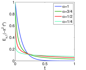
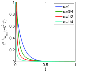
(a) $E_{\alpha,1}(-\pi^{2}t^{\alpha})$	(b) $t^{\alpha-1}E_{\alpha,\alpha}(-\pi^{2}t^{\alpha})$

Figure 1. The profiles of Mittag-Leffler functions (a) $E_{\alpha,1}(-\pi^{2}t^{\alpha})$ and (b) $t^{\alpha-1}E_{\alpha,\alpha}(-\pi^{2}t^{\alpha})$. The value $\pi^{2}$ is the first Dirichlet eigenvalue of the negative Laplacian on the interval $(0,1)$.

The distribution of zeros of the Mittag-Leffer function $E_{\alpha,\beta}(z)$ is of immense interest, especially in the related Sturm-Liouville problem; see Section 4.1 below. The case of $\beta=1$ was first studied by Wiman [104]. It was revisited by Djrbashian [21], and many deep results were derived, especially for the case of $\alpha=2$. There are many further refinements [93]; see [83] for an updated account.

2.2. Wright function

The Wright function $W_{\rho,\mu}(z)$ is defined by [106, 107]

$$W_{\rho,\mu}(z)=\sum_{k=0}^{\infty}\frac{z^{k}}{k!\Gamma(\rho k+\mu)},\qquad\mu,\ \rho\in\mathbb{R},\ \rho>-1,\quad z\in\mathbb{C}.$$

This is an entire function of order $1/(1+\rho)$ [30, Theorem 2.4.1]. It was first introduced in connection with a problem in number theory by Edward M. Wright, and revived in recent years since it appears as the fundamental solution for FDEs [69]. The Wright function $W_{\rho,\mu}(z)$ has the following the asymptotic expansion in one sector containing the negative real axis $\mathbb{R}^{-}$ [67, Theorem 3.2]. Like before, the exponential asymptotics can be used to deduce the distribution of its zeros [66].

Lemma 2.2.

Let $-1<\rho<0$, $y=-z$, $\mathrm{arg}(z)\leq\pi$, $-\pi<\mathrm{arg}(y)\leq\pi$, $|\mathrm{arg}(y)|\leq\min(3\pi(1+\rho)/2,\pi)-\epsilon$, $\epsilon>0$. Then

$$W_{\rho,\mu}(z)=Y^{1/2-\mu}e^{-Y}\left\{\sum_{m=0}^{M-1}A_{m}Y^{-m}+O(Y^{-M})\right\},\ \ Y\to\infty,$$

where $Y=(1+\rho)((-\rho)^{-\rho}y)^{1/(1+\rho)}$ and the coefficients $A_{m}$, $m=0,1,\ldots$ are defined by the asymptotic expansion

$$\frac{\Gamma(1-\mu-\rho t)}{2\pi(-\rho)^{-\rho t}(1+\rho)^{(1+\rho)(t+1)}\Gamma(t+1)} =\sum_{m=0}^{M-1}\frac{(-1)^{m}A_{m}}{\Gamma((1+\rho)t+\mu+\frac{1}{2}+m)}$$

$$\qquad+O\left(\frac{1}{\Gamma((1+\rho)t+\beta+\tfrac{1}{2}+M)}\right),$$

valid for $\mathrm{arg}(t),\mathrm{arg}(-\rho t)$, and $\mathrm{arg}(1-\mu-\rho t)$ all lying between $-\pi$ and $\pi$ and $t$ tending to infinity.

The Wright function $W_{\rho,\mu}(z)$, $-1<\rho<0$, decays exponentially on the negative real axis $\mathbb{R}^{-}$, in a manner similar to the exponential function $e^{z}$, but at a different decay rate. Its special role in fractional calculus is underscored by the fact that it forms the free-space fundamental solution $K_{\alpha}(x,t)$ to the one-dimensional time fractional diffusion equation [69] by

(2.2) $$K_{\alpha}(x,t)=\frac{1}{2t^{\frac{\alpha}{2}}}W_{-\frac{\alpha}{2},1-\frac{\alpha}{2}}\left(-|x|/t^{\alpha/2}\right).$$

The multidimensional case is more complex and involves further special functions, in particular, the Fox H function [91, 54]. For $\alpha=1$, the formula (2.2) recovers the familiar free-space fundamental solution for the one-dimensional heat equation, i.e.,

$$K(x,t)=\frac{1}{2\sqrt{\pi t}}e^{-\frac{x^{2}}{4t}},$$

which is a Gaussian distribution in $x$ for any $t>0$. In the fractional case, the fundamental solution $K_{\alpha}(x,t)$ exhibits quite different behavior than the heat kernel. To see this, we show the profile of $K_{\alpha}(x,t)$ in Fig. 2 for several $\alpha$ values; see Appendix A.1 for a brief description of the computational details. For any $0<\alpha<1$, $K_{\alpha}(x,t)$ decays slower at a polynomial rate as the argument $|x|/t^{\alpha/2}$ tends to infinity, i.e., having a long tail, when compared with the Gaussian density. The long tail profile is one of distinct features of slow diffusion [5]. Further, for any $\alpha<1$, the profile is only continuous but not differentiable at $x=0$. The kink at the origin implies that the solution operator to time fractional diffusion may only have a limited smoothing property.

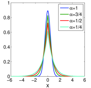
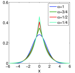
(a) $t=0.1$	(b) $t=1$

Figure 2. The profile of the fundamental solution $K_{\alpha}(x,t)$ at (a) $t=0.1$ and (b) $t=1$.

2.3. Singular value decomposition

We shall follow the well-established practice in the inverse problem community, i.e., using the singular value decomposition, as the main tool for numerically analyzing the problem behavior [32]. Specifically, we shall numerically compute the forward map $F$, and analyze its behavior to gain insights into the inverse problem. Given a matrix $\mathbf{A}\in\mathbb{R}^{n\times m}$, its singular value decomposition is given by

$$\mathbf{A}=\mathbf{U}\Sigma\mathbf{V}^{\mathrm{t}},$$

where $\mathbf{U}=[\mathbf{u}_{1}\ \ldots\ \mathbf{u}_{n}]\in\mathbb{R}^{n\times n}$ and $\mathbf{V}=[\mathbf{v}_{1}\ \ldots\ \mathbf{v}_{m}]\in\mathbb{R}^{m\times m}$ are column orthonormal matrices, and $\Sigma\in\mathbb{R}^{n\times m}=\mathrm{diag}(\sigma_{1},\ldots,\sigma_{r},0,\ldots,0)$ is a diagonal matrix, with the diagonal elements $\{\sigma_{i}\}$ being nonnegative and listed in a descending order $\sigma_{1}>\ldots>\sigma_{r}>0$, and $r$ being the (numerical) rank of the matrix $\mathbf{A}$. The diagonal element $\sigma_{i}$ is known as the $i$th singular value, and the corresponding columns of $\mathbf{U}$ and $\mathbf{V}$, i.e., $\mathbf{u}_{i}$ and $\mathbf{v}_{i}$, are called the left and right singular vectors, respectively.

One simple measure of the conditioning of a linear inverse problem $\mathbf{Ax}=\mathbf{b}$ is the condition number $\mathrm{cond}(\mathbf{A})$, which is defined as the ratio of the largest to the smallest nonzero singular value, i.e.,

$$\mathrm{cond}(\mathbf{A})=\sigma_{1}/\sigma_{r}.$$

In particular, if the condition number is small, then the data error will not be amplified much. In the case of a large condition number, the issue is more delicate: it may or may not amplify the data perturbation greatly. A more complete picture is provided by the singular value spectrum $(\sigma_{1},\sigma_{2},\ldots,\sigma_{r})$. Especially, a singular value spectrum gradually decaying to zero without a clear gap is characteristic of many discrete ill-posed problems, which is reminiscent of the spectral behavior of compact operators. We shall adopt these simple tools to analyze related inverse problems below.

In addition, using singular value decomposition and regularization techniques, e.g. Tikhonov regularization or truncated singular value decomposition, one can conveniently obtain numerical reconstructions, even though this might not be the most efficient way to do so. However, we shall not delve into the extremely important question of practical reconstructions, since it relies heavily on a priori knowledge on the sought for solution and the statistical nature (Gaussian, Poisson, Laplace …) of the contaminating noise in the data, which will depend very much on the specific application. We refer interested readers to the monographs [26, 92, 41] and the survey [49] for updated accounts on regularization methods for constructing stable reconstructing procedures and efficient computational techniques. We will also briefly mention below related works on the application of regularization techniques to inverse problems for FDEs.

3. Inverse problems for time fractional diffusion

In this section, we consider several model inverse problems for the following one-dimensional time fractional diffusion equation on the unit interval $\Omega=(0,1)$:

(3.1) $$\partial_{t}^{\alpha}u-u_{xx}+qu=f\quad\mbox{ in }\Omega\times(0,T],$$

with the fractional order $\alpha\in(0,1)$, the initial condition $u(0)=v$ and suitable boundary conditions. Although we consider only the one-dimensional model, the analysis and computation in this part can be extended into the general multi-dimensional case, upon suitable modifications. Recall that $\partial_{t}^{\alpha}u$ denotes the Djrbashian-Caputo fractional derivative of order $\alpha$ with respect to time $t$. For $\alpha=1$, the fractional derivative $\partial_{t}^{\alpha}u$ coincides with the usual first-order derivative $u^{\prime}$, and accordingly, the model (3.1) reduces to the classical diffusion equation. Hence it is natural to compare inverse problems for the model (3.1) with that for the standard diffusion equation. We shall discuss the following four inverse problems, i.e., the backward problem, sideways problem, inverse source problem and inverse potential problem. In the first three cases, we shall assume a zero potential $q=0$. We will aslo discuss the solution of an inverse coefficient problem using fractional calculus.

3.1. Backward fractional diffusion

First we consider the time fractional backward diffusion. By the linearity of the inverse problem, we may assume that equation (3.1) is prescribed with a homogeneous Dirichlet boundary condition, i.e., $u=0$ at $x=0,1$, and the initial condition $u(0)=v$. Then the inverse problem reads: given the final time data $g=u(T)$, find the initial condition $v$. It arises in, for example, the determination of a stationary contaminant source in underground fluid flow.

To gain insight, we apply the separation of variables. Let $\{(\lambda_{j},\phi_{j})\}$, with $\lambda_{j}=(j\pi)^{2}$ and $\phi_{j}=\sqrt{2}\sin j\pi x$, be the Dirichlet eigenpairs of the negative Laplacian on the interval $\Omega$. The eigenfunctions $\{\phi_{j}\}$ form an orthonormal basis of the $L^{2}(\Omega)$ space. Then using the Mittag-Leffler function $E_{\alpha,\beta}(z)$ defined in (2.1), the solution $u$ to equation (3.1) can be expressed as

$$u(x,t)=\sum_{j=1}^{\infty}E_{\alpha,1}(-\lambda_{j}t^{\alpha})(v,\phi_{j})\phi_{j}(x).$$

Therefore, the final time data $g=u(T)$ is given by

$$g(x)=\sum_{j=1}^{\infty}E_{\alpha,1}(-\lambda_{j}T^{\alpha})(v,\phi_{j})\phi_{j}(x).$$

It follows directly that the initial data $v$ is formally given by

$$v=\sum_{j=1}^{\infty}\frac{(g,\phi_{j})}{E_{\alpha,1}(-\lambda_{j}T^{\alpha})}\phi_{j}.$$

Since the function $E_{\alpha,1}(-t)$ is completely monotone on the positive real axis $\mathbb{R}^{+}$ [82] for any $\alpha\in(0,1]$, the denominator in the representation does not vanish. In case of $\alpha=1$, the formula reduces to the familiar expression

$$v=\sum_{j=1}^{\infty}e^{\lambda_{j}T}(g,\phi_{j})\phi_{j}.$$

This formula shows clearly the well-known severely ill-posed nature of the backward diffusion problem: the perturbation in the $j$th Fourier mode $(g,\phi_{j})$ of the (noisy) data $g$ is amplified by an exponentially growing factor $e^{\lambda_{j}T}$, which can be astronomically large, even for a very small index $j$, if the terminal time $T$ is not very small. Hence it is always severely ill-conditioned and we must multiply the $j$th Fourier mode of the data $g$ by a factor $e^{\lambda_{j}T}$ in order to recover the corresponding mode of the initial data $v$

In the fractional case, by Lemma 2.1, the Mittag-Leffler function $E_{\alpha,1}(z)$ decays only linearly on the negative real axis $\mathbb{R}^{-}$, and thus the multiplier $1/E_{\alpha,1}(-\lambda_{j}T^{\alpha})$ grows only linearly in $\lambda_{j}$, i.e., $1/E_{\alpha,1}(-\lambda_{j}T^{\alpha})\sim\lambda_{j}$, which is very mild compared to the exponential growth $e^{\lambda_{j}T}$ for the case $\alpha=1$, and thus the fractional case is only mildly ill-posed. Roughly, the $j$th Fourier mode of the initial data $v$ now equals the $j$th mode of the data $g$ multiplied by $\lambda_{j}$. More precisely, it amounts to the loss of two spatial derivatives [88, Theorem 4.1]

(3.2) $$\|v\|_{L^{2}(\Omega)}\leq c\|u(T)\|_{H^{2}(\Omega)}.$$

Intuitively, the history mechanism of the anomalous diffusion process retains the complete dynamics of the physical process, including the initial data, and thus it is much easier to go backwards to the initial state $v$. This is in sharp contrast to the classical diffusion, which has only a short memory and loses track of the preceding states quickly. This result has become quite well-known in the inverse problems community and has contributed to a belief that “inverse problems for FDEs are less ill-conditioned than their classical counterparts” – throughout this paper we will see that this conclusion as a general statement can be quite far from the truth.

Does this mean that for all terminal time $T$ the fractional case is always less ill-posed than the classical one? The answer is yes, in the sense of the norm on the data space in which the data $g$ lies. Does this mean that from a computational stability standpoint that one can always solve the backward fractional problem more effectively than for the classical case? The answer is no, and the difference can be substantial. To illustrate the point, let $J$ be the highest frequency mode required of the initial data $v$ and assume that we believe we are able to multiply the first $J$ modes $g_{j}=(g,\phi_{j})$, $j=1,2,\ldots,J$, by a factor no larger than $M$ (which roughly assumes that the noise levels in both cases are comparable). By the monotonicity of the function $E_{\alpha,1}(-t)$ in $t$, it suffices to examine the $J$th mode. For the heat equation $v_{J}:=(v,\phi_{J})=e^{\lambda_{J}T}g_{J}$ and provided that $T=T_{J}<\lambda_{J}/\log{M}$ this is feasible. For a fixed $J$, if $T_{\alpha}^{\star}$ denotes the point where

$$e^{-\lambda_{J}T_{\alpha}^{\star}}=E_{\alpha,1}(-\lambda_{J}T_{\alpha}^{\star}),$$

then in the fractional case for $T<T_{\alpha}^{\star}$ the growth factor on $g_{J}$ will exceed $M$ for any $T<T_{\alpha}^{\star}$. In Table 1 below, we present the critical value $T_{\alpha}^{\star}$ for several values of the fractional order $\alpha$ and the maximum number of modes $J$. The numbers in the table are very telling. For example, for the case $J=5$, $\alpha=1/4$ and $T=0.02$ (which is approximately one half the value of $T_{\alpha}^{\star}$), the growth factor is about $1.6$ for the heat equation but about $113$ for the fractional case. With $J=10$ and $\alpha=1/4$ and $T=T_{\alpha}^{\star}$ the growth factor is around $336$. If $T=T_{\alpha}^{\star}/10$ then it has again dropped to less than $2$ for the heat equation but about $190$ for the fractional case. Of course, for $T>T_{\alpha}^{\star}$ the situation completely reverses. With $J=10$, $\alpha=1/4$ and $T=10\,T_{\alpha}^{\star}$ the growth factor is a possibly workable value of around $600$; while for the heat equation it is greater than $10^{25}$. We reiterate that the apparent contradiction between the theoretical ill-conditioning and numerical stability is due to the spectral cutoff present in any practical reconstruction procedure.

Table 1. The critical values $T_{\alpha}^{*}$ for fractional backward diffusion.

$\alpha\backslash J$	3	5	10
1/4	0.0442	0.0197	0.0059
1/2	0.0387	0.0163	0.0049
3/4	0.0351	0.0142	0.0040

Next we examine the influence of the fractional order $\alpha$ on the inversion step more closely. To this end, we expand the initial condition $v$ in the piecewise linear finite element basis functions defined on a uniform partition of the domain $\Omega=(0,1)$ with 100 grid points. Then we compute the discrete forward map $F$ from the initial condition to the final time data $g=u(T)$, defined on the same mesh. Numerically, this can be achieved by a fully discrete scheme based on the L1 approximation in time and the finite difference method in space; see Appendix A.2 for a description of the numerical method. The ill-posed behavior of the discrete inverse problem is then analyzed using singular value decomposition. A similar experimental setup will be adopted for other examples below.

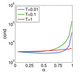
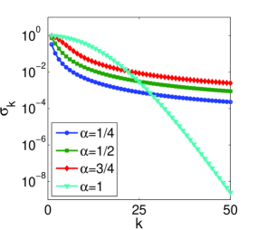
(a) condition number	(b) singular value spectrum

Figure 3. (a) The condition number v.s. the fractional order $\alpha$, and (b) the singular value spectrum at $T=0.01$ for the backward fractional diffusion. We only display the first 50 singular values.

The numerical results are shown in Fig. 3. The condition number of the (discrete) forward map $F$ stays mostly around $O(10^{4})$ for a fairly broad range of $\alpha$ values, which holds for all three different terminal times $T$. This can be attributed to the fact that for any $\alpha\in(0,1)$, backward fractional diffusion amounts to a two spacial derivative loss, cf. (3.2). Unsurprisingly, as the fractional order $\alpha$ approaches unity, the condition number eventually blows up, recovering the severely ill-posed nature of the classical backward diffusion problem, cf. Fig. 3(a). Further, we observe that the smaller is the terminal time $T$, the quicker is the blowup. The precise mechanism for this observation remains unclear. Interestingly, the condition number is not monotone with respect to the fractional order $\alpha$, for a fixed $T$. This might imply potential nonuniqueness in the simultaneous recovery of the fractional order $\alpha$ and the initial data $v$. The singular value spectra at $T=0.01$ are shown in Fig. 3(b). Even though the condition numbers for $\alpha=1/4$ and $\alpha=1/2$ are quite close, their singular value spectra actually differ by a multiplicative constant, but their decay rates are almost identical, thereby showing comparable condition numbers. This shift in singular value spectra can be explained by the local decay behavior of the Mittag-Leffler function, cf. Fig. 1(a): the smaller is the fractional order $\alpha$, the faster is the decay around $t=0$.

Even though the condition number is very informative about the (discretized) problem, it does not provide a full picture, especially when the condition number is large, and the singular value spectrum can be far more revealing. The spectra for two different $\alpha$ values are given in Fig. 4. At $\alpha=1/2$, the singular values decay at almost the same algebraic rate, irrespective of the terminal time $T$. This is expected from the two-derivative loss for any $\alpha<1$. However, for $\alpha=1$, the singular values decay exponentially, and the decay rate increases dramatically with the increase of the terminal time $T$. For $T=0.001$, there are a handful of “significant” singular values, say above $10^{-3}$, but when the time $T$ increases to $T=1$, there is only one meaningful singular value remaining. The distribution of the singular values has important practical consequences. For a small time $T$, the first few singular values for the classical diffusion case actually might be much larger than that for the fractional case, which indicates that the classical case is actually numerically much easier to recover in this regime, concurring with the observations drawn from Table 1. For example, at $T=0.001$, the first twenty singular values are larger than the fractional counterpart, cf. Fig. 3(b), and hence, the first twenty modes, i.e., left singular vectors, are more stable in the reconstruction procedure.

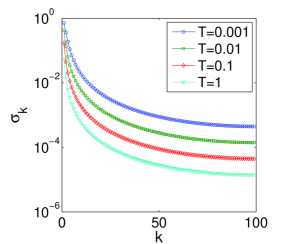
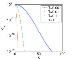
(a) $\alpha=1/2$	(b) $\alpha=1$

Figure 4. The singular value spectrum of the forward map $F$ from the initial data to the final time data, for (a) $\alpha=1/2$ and (b) $\alpha=1$, at four different times for the time fractional backward diffusion.

The mathematical model (3.1) is rescaled with a unit diffusion coefficient. In practice, there is always a diffusion coefficient $\sigma$ in the elliptic operator, i.e.,

$$\partial_{t}^{\alpha}u-\nabla\cdot(\sigma\nabla u)+qu=f.$$

For example, the thermal conductivity $\sigma$ of the gun steel at moderate temperature is about $1.8\times 10^{-5}\ \mathrm{m}^{2}/\mathrm{s}$ [11] and the diffusion coefficient of the oxygen in water at 25 Celsius is $2.10\times 10^{-5}\ \mathrm{cm}^{2}/\mathrm{s}$ [18]. Mathematically, this does not change the ill-posed nature of the inverse problem. However, the presence of a diffusion coefficient $\sigma$ has important consequence: it enables the practical feasibility of the classical backward diffusion problem (and likely for many other inverse problems for the diffusion equation). Physically, a constant conductivity $\sigma$ amounts to rescaling the final time $T$ by $T^{\prime}=T/\sigma$. In the fractional case, a similar but nonlinear scaling law $T^{\prime}=T/\sigma^{1/\alpha}$ remains valid.

Numerically, time fractional backward diffusion has been extensively studied. Liu and Yamamoto [65] proposed a numerical scheme for the one-dimensional fractional backward problem based on the quasi-reversibility method [57], and derived error estimates for the approximation, under a priori smoothness assumption on the initial condition. This represents one of the first works on inverse problems in anomalous diffusion. Later, Wang and Liu [99] studied total variation regularization for two-dimensional fractional backward diffusion, and analyzed its well-posedness of the optimization problem and the convergence of an iterative scheme of Bregman type. Wei and Wang [102] developed a modified quasi-boundary value method for the problem in a general domain, and established error estimates for both a priori and a posteriori parameter choice rules. In view of better stability results in the fractional case, one naturally expects better error estimates than the classical diffusion equation, which is confirmed by these studies.

3.2. Sideways fractional diffusion

Next we consider the sideways problem for time fractional diffusion. There are several possible formulations, e.g., the quarter plane and the finite space domain. The quarter plane sideways fractional diffusion problem is as follows. Let $u(x,t)$ be defined in $(0,\infty)\times(0,\infty)$ by

$$\partial^{\alpha}_{t}u-u_{xx}=0,\qquad x>0,\ t>0,$$

and the boundary and initial conditions

$$u(x,0)=0\quad\mbox{and}\quad u(0,t)=f(t),$$

where we assume $|u(x,t)|\leq c_{1}e^{c_{2}x^{2}}$. We do not know the left boundary condition $f$, but are able to measure $u$ at an intermediate point $x=L>0$, $h(t)=u(L,t)$. The inverse problem is: given the (noisy) data $h$, find the boundary condition $f$. The solution $u$ of the forward problem is given by a convolution integral with the kernel being the spatial derivative $K_{\alpha,x}(x,s)$ of the fundamental solution $K_{\alpha}(x,s)$, cf. (2.2), by

$$u(x,t)=\int_{0}^{t}K_{\alpha,x}(x,t-s)f(s)ds.$$

This representation is well known for the case $\alpha=1$, and it was first derived by Carasso [11]; see also [8] for related discussions. It leads to a convolution integral equation for the unknown $f$ in terms of the given data $h$

$$h(t)=\int_{0}^{t}R_{\alpha}(t-s)f(s)ds,$$

where the convolution kernel $R_{\alpha}(s)$ is given by a Wright function in the form

$$R_{\alpha}(s) =\frac{1}{2s^{\alpha}}W_{-\frac{\alpha}{2},2-\frac{\alpha}{2}}(-Ls^{-\alpha/2})$$

$$=\sum_{k=0}^{\infty}\frac{(-L)^{k}}{k!\,\Gamma(-\frac{\alpha}{2}k+2-\frac{\alpha}{2})}\,s^{-k\frac{\alpha}{2}-\alpha}.$$

In case of $\alpha=1$, i.e., classical diffusion, the kernel $R(s)$ is given explicitly by

$$R(s)=\frac{L}{2\sqrt{\pi}}s^{-\frac{3}{2}}e^{-\frac{L^{2}}{4s}}\in C^{\infty}(0,\infty).$$

Since all its derivatives vanish at $s=0$, the classical theory of Volterra integral equations of the first kind [56] implies the extreme ill-conditioning of the problem. This is not surprising: We are, after all, mapping a function $f\in C^{0}(0,\infty)$ to an element in $C^{\infty}(0,\infty)$. The conditioning of the time fractional sideways problem again depends on the convolution kernel $R_{\alpha}$ and its derivatives at $s=0$ and in this case is the value of the Wright function $W_{-\alpha/2,2-\alpha/2}(-z)$ and its derivatives as $z\to\infty$. These are again zero (in fact the Wright function $W_{-\alpha/2,2-\alpha/2}(z)$ also decays exponentially to zero for large negative arguments, cf. Lemma 2.2), and thus the fractional sideways problem is also severely ill-posed. However, this analysis does not show their difference in the degree of ill-posedness: even though both are severely ill-posed, their practical computational behavior can still be quite different, as we shall see below.

To see their difference in the degree of ill-posedness, we examine another variant of the sideways problem on a finite interval $\Omega=(0,1)$, with Cauchy data prescribed on the axis $x=0$, i.e. given zero initial condition $u_{0}=u(x,0)=0$, recovering $h=u(1,t)$ from the lateral Cauchy data at $x=0$:

$$u(0,t)=f(t),\ \ u_{x}(0,t)=g(t),\ \ t\geq 0$$

This problem is also known as the lateral Cauchy problem in the literature. In the case $\alpha=1$, it is known that the inverse problem is severely ill-posed [8, 33]. To gain insight into the fractional case, we apply the Laplace transform. With $\ \widehat{}\$ being the Laplace transform in time, and noting the Laplace transform of the Caputo derivative $\mathcal{L}(\partial_{t}^{\alpha}u)=z^{\alpha}\widehat{u}(z)-z^{\alpha-1}u_{0}$ [53, Lemma 2.24], we deduce

$$z^{\alpha}\widehat{u}(x,z)-\widehat{u}_{xx}(x,z)=0,\ \ \widehat{u}(0)=\widehat{f},\ \ \widehat{u}_{x}(0)=\widehat{g}.$$

The general solution $\widehat{u}$ is given by $\widehat{u}(x,z)=\widehat{f}\cosh z^{\alpha/2}x+\widehat{g}\frac{\sinh z^{\alpha/2}x}{z^{\alpha/2}x}$ and thus the solution $\widehat{h}(z)=\widehat{u}(1,z)$ at $x=1$ is given by

$$\widehat{h}=\widehat{f}\cosh z^{\alpha/2}+\widehat{g}\frac{\sinh z^{\alpha/2}}{z^{\alpha/2}}.$$

The solution $h(t)$ can then be recovered by an inverse Laplace transform

(3.3) $$h(t)=\frac{1}{2\pi\mathrm{i}}\int_{Br}\widehat{h}e^{zt}dz,$$

where $Br=\{z\in\mathbb{C}:\Re z=\sigma,\sigma>0\}$ is the Bromwich path. Upon deforming the contour suitably, this formula will allow developing an efficient numerical scheme for the sideways problem via quadrature rules [103], provided that the lateral Cauchy data is available for all $t>0$. The expression (3.3) indicates that, in the fractional case, the sideways problem still suffers from severe ill-posedness in theory, since the high frequency modes of the data perturbation are amplified by an exponentially growing multiplier $e^{z^{\alpha/2}}$. However, numerically, the degree of ill-posedness decreases dramatically as the fractional order $\alpha$ decreases from unity to zero, since as $\alpha\to 0^{+}$, the multipliers are growing at a much slower rate, and thus we have a better chance of recovering many more modes of the boundary data. In other words, both the classical and fractional sideways problems are severely ill-posed in the sense of error estimates between the norms in the data and unknowns; but with a fixed frequency range, the behavior of the time fractional sideways problem can be much less ill-posed. Hence, anomalous diffusion mechanism does help substantially since much more effective reconstructions are possible in the fractional case.

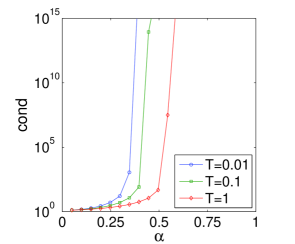
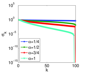
(a) condition number	(b) singular value spectrum

Figure 5. (a) The condition number and (b) singular value spectrum at $T=1$ for the time fractional sideways problem.

Next we illustrate the point numerically. The numerical results for the sideways problem are given in Fig. 5. It is observed that the degree of ill-posedness of the finite-dimensional discretized version of the inverse problem indeed decreases dramatically with the decrease of the fractional order $\alpha$, cf. Fig. 5(a), which agrees well with the preceding discussions. Surprisingly, for $T=1$ there is a sudden transition around $\alpha=1/2$, below which the sideways problem behaves as if nearly well-posed, but above which the conditioning deteriorates dramatically with the increase of the fractional order $\alpha$ and eventually it recovers the properties of the classical sideways problem. Similar transitions are observed for other terminal times. This might be related to the discrete setting, for which there is an inherent frequency cutoff. Further, as the fractional order $\alpha$ approaches zero, the problem reaches a quasi-steady state much quicker and thus the forward map $F$ can have only fairly localized elements along the main diagonal. To give a more complete picture, we examine the singular value spectrum in Fig. 5(b). Unlike the backward diffusion problem discussed earlier, the singular values are actually decaying only algebraically, even for $\alpha=1$, and then there might be a few tiny singular values contributing to the large condition number. The larger is the fractional order $\alpha$, the more tiny singular values are in the spectrum. Hence, in the discrete setting, even for $\alpha=3/4$, the problem is still nearly well-posed, despite the large apparent condition number, since a few tiny singular values with a distinct gap from the rest of the spectrum are harmless in most regularization techniques.

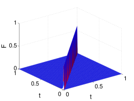
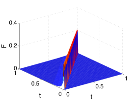
(a) $\alpha=1/4$	(b) $\alpha=1/2$
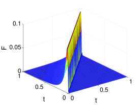
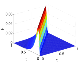
(c) $\alpha=3/4$	(d) $\alpha=1$

Figure 6. The Jacobian map $F$ for $\alpha=1/4$, $1/2$, $3/4$ and $1$, from the interval $(0,1)$ itself.

Physically this can also be observed in Fig. 6, where the forward map $F$ is from the Dirichlet boundary condition $x=1$ to the flux boundary condition at $x=0$, in a piecewise linear finite element basis. Pictorially, the forward map $F$ is only located in the upper left corner and has a triangular structure, which reflects the casual or Volterra nature of the sideways problem for the fractional diffusion equation. We note that the casual structure should be utilized in developing reconstruction techniques, via, e.g., Lavrentiev regularization [56]. For small $\alpha$ values, e.g., $\alpha=1/4$, the finite element basis at the right end point $x=1$ is almost instantly transported to the left end point $x=0$, whose magnitude is slightly decreased, but with little diffusive effect, resulting a diagonally dominant forward map. However, as the fractional order $\alpha$ increases towards unity, the diffusive effect eventually kicks in, and the information spreads over the whole interval. Further, for large $\alpha$ values, it takes much longer time to reach the other side and there is a lag of information arrival, which explains the presence of tiny singular values. The larger is the fractional order $\alpha$, the smaller is the magnitude, i.e., the less is the amount of the information reached the other side. Hence, one feasible approach is to recover only the boundary condition over a smaller subinterval of the measurement time interval. This idea underlies one popular engineering approach, the sequential function specification method [4, 64].

The sideways problem for the classical diffusion has been extensively studied, and many efficient numerical methods have been developed and analyzed [11, 8, 24, 25]. In the fractional case, however, there are only a few works on numerical schemes, mostly for one-dimensional problems, and there seems no theoretical study on stability etc. Murio [76, 77] developed several numerical schemes, e.g., based on space marching and finite difference method, for the sideways problem, but without any analysis. Qian [85] discussed about the ill-posedness of the quarter plane formulation of the sideways problem using the Fourier analysis, based on which a mollifier method was proposed, with error estimates provided. In [87], the recovery of a nonlinear boundary condition from the lateral Cauchy data was studied using an integral equation approach, and a convergent fixed point iteration method was suggested. The influence of the imprecise specification of the fractional order $\alpha$ on the reconstruction was examined. Zheng and Wei [113] proposed a mollification method for the quarter plane formulation of the sideways problem, by convoluting the fractional derivative with a smooth kernel, and derived error estimates for the approximation, under a prior bounds on the solution. The Cauchy problem of the time fractional diffusion has been numerically studied in [114]. In particular, with the separation of variables, a Volterra integral equation reformulation of the problem was derived, from which the ill-posedness of the Cauchy problem follows directly. All these works are concerned with the one-dimensional case, and the high dimensional case has not been studied.

3.3. Inverse source problem

A third classical linear inverse problem for the diffusion equation is the inverse source problem, i.e., the recovery of the source term $f$ from lateral boundary data or final time data. Clearly, one piece of boundary data or final time data alone is insufficient to uniquely determine a general source term, due to dimensionality disparity. To restore the possible uniqueness, as usual, we look for only a space- or time-dependent component of the source term $f$. With different combinations of the data and source term, we get several different (and not equivalent) formulations of the inverse source problems. Below we examine several of them briefly. By the linearity of the forward problem, we without loss of generality, assume a zero initial data $v=0$ and a zero potential $q=0$ throughout this part.

First, suppose we can measure the solution $u$ at the final time $t=T$, and aim at recovering either a space dependent or time dependent component of the source term $f$. Like before, we resort to the separation of variables. For the case of a space dependent only source term $f(x)$, the solution $u$ to the forward problem is given by

$$u(t) =\sum_{j=1}^{\infty}\int_{0}^{t}(t-\tau)^{\alpha-1}E_{\alpha,\alpha}(-\lambda_{j}(t-\tau)^{\alpha})(f,\phi_{j})\phi_{j}d\tau$$

$$=\sum_{j=1}^{\infty}\lambda_{j}^{-1}(1-E_{\alpha,1}(-\lambda_{j}t^{\alpha}))(f,\phi_{j})\phi_{j}.$$

Hence the measured data $g=u(T)$ is given by

$$g=\sum_{j=1}^{\infty}\frac{1}{\lambda_{j}}(1-E_{\alpha,1}(-\lambda_{j}T^{\alpha}))(f,\phi_{j})\phi_{j}.$$

By taking inner product with $\phi_{j}$ on both sides, we arrive at the following representation of the source term $f$ in terms of the measured data $g$

(3.4) $$f=\sum_{j=1}^{\infty}\lambda_{j}\frac{(g,\phi_{j})}{1-E_{\alpha,1}(-\lambda_{j}T^{\alpha})}\phi_{j}.$$

By the complete monotonicity of the Mittag-Leffler function $E_{\alpha,1}(-t)$ on the positive real axis $\mathbb{R}^{+}$ [82], we deduce

$$1>E_{\alpha,1}(-\lambda_{1}T^{\alpha})>E_{\alpha,1}(-\lambda_{2}T^{\alpha}),$$

and thus the formula (3.4) is well defined for any $T>0$, and gives the precise condition for the existence of a source term. Even with a modest value of the terminal time $T$, the factor $1-E_{\alpha,1}(-\lambda_{1}T^{\alpha})$ is close to unity for all small $\alpha$ values, especially for those close to zero. Each frequency component $(f,\phi_{j})$ differs from $(g,\phi_{j})$ essentially by a factor $\lambda_{j}$, which amounts to two derivative loss in space. Actually one can show

$$\|f\|_{L^{2}(\Omega)}\leq c\|g\|_{H^{2}(\Omega)}.$$

This behavior is identical with that for the backward fractional diffusion. The statement holds also for the inverse source problem for the classical diffusion case. This is not surprising, since with a space dependent source term $f$, the solution $u$ to the forward problem can be split into the steady solution $u_{s}$ and the decaying solution $u_{d}$, i.e., $u=u_{s}+u_{d}$, where $u_{s}$ and $u_{d}$ solve

$$-u_{s}^{\prime\prime}=f,\ \ u_{s}(0)=u_{s}(1)=0,$$

and

$$\partial_{t}^{\alpha}u_{d}-u_{d,xx}=0,\ \ u_{d}(0,x)=f(x),\ \ u_{d}(0,t)=u_{d}(1,t)=0,$$

respectively. By the decay behavior of the solution $u_{d}$, the steady state component $u_{s}$ is dominating, which amounts to a two spatial derivative loss. This is fully confirmed by the numerical experiments, cf. Fig. 7. It is observed that the condition number is almost independent of the fractional order $\alpha$, and it is of order $O(10^{3})$, reflecting the mildly ill-posed nature of the inverse problem. In particular, for large terminal time $T$, the singular value spectra are almost identical for all fractional orders, decaying to zero at an algebraic rate, cf. Fig. 7(b).

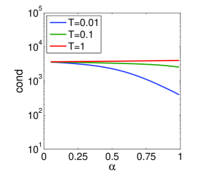
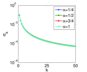
(a) condition number	(b) singular value spectrum

Figure 7. Numerical results for the inverse source problem with final time data and a space dependent source term. (a) The condition number v.s. the fractional order $\alpha$, and (b) singular value spectrum at $T=1$.

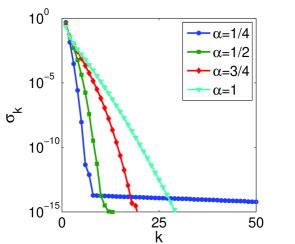
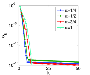
(a) $T=0.01$	(b) $T=1$

Figure 8. The singular value spectrum at two different terminal times for the inverse source problem with a final time data at terminal time $T$, and $f(x,t)=xp(t)$, an unknown time dependent component $p(t)$.

Next we turn to the time dependent case, i.e., seeking a source term $f$ of the form $f(x,t)=p(t)q(x)$, with a known spacial component $q(x)$, from the final time data $g=u(T)$. Mathematically, the inverse problem even for the classical diffusion equation has not been completely analyzed. The inclusion of a nontrivial term $q(x)$ is important since without this there is nonuniqueness. To see this, we take $u$ to satisfy $u_{t}-u_{xx}=f(t)$ on $(0,1)\times(0,T)$ with initial data $u(x,0)=1$ and a homogeneous Neumann boundary condition $-u_{x}(0,t)=u_{x}(1,t)=0$. Then one solution satisfying $u(x,T)=g(x)=1$ is given by $u(x,t)=1$ and $f\equiv 0$, but another is $u(x,t)=\cos(2\pi t/T)$ and $f=(-2\pi/T)\sin(2\pi t/T)$. Likewise, in the fractional case, we can take $u=\cos(2\pi t/T)$ for the second solution and define $f$ to be its $\alpha$th order Djrbashian-Caputo fractional derivative in time.

Like previously, the solution $u$ to (3.1) is given by

$$u(t) =\sum_{j=1}^{\infty}\int_{0}^{t}(t-\tau)^{\alpha-1}E_{\alpha,\alpha}(-\lambda_{j}(t-\tau)^{\alpha})p(\tau)d\tau(q,\phi_{j})\phi_{j}.$$

Hence the measured data $g(x)=u(x,T)$ is given by

$$g(x)=\sum_{j=1}^{\infty}\int_{0}^{T}(T-\tau)^{\alpha-1}E_{\alpha,\alpha}(-\lambda_{j}(T-\tau)^{\alpha})p(\tau)d\tau(q,\phi_{j})\phi_{j}(x).$$

By taking inner product with $\phi_{j}$ on both sides, we deduce

$$(g,\phi_{j})=(q,\phi_{j})\int_{0}^{T}(T-\tau)^{\alpha-1}E_{\alpha,\alpha}(-\lambda_{j}(T-\tau)^{\alpha})p(\tau)d\tau.$$

In the case of $\alpha=1$, the formula recovers the relation

$$(g,\phi_{j})=(q,\phi_{j})\int_{0}^{T}e^{-\lambda_{j}(T-\tau)}p(\tau)d\tau,$$

which resembles a finite-time Laplace transform or moment problem, and thus severely smoothing, which renders the inverse source problem severely ill-posed. Intuitively, the term $e^{-\lambda_{j}(T-t)}$ can only pick up the information for $t$ close to the terminal time $T$, and for $t$ away from $T$, the information is severely damped, especially for high frequency modes, which leads to the severely ill-posed nature of the inverse problem. In the fractional case, the forward map $F$ from the unknown to the data is clearly compact, and thus the problem is still ill-posed. However, the kernel $t^{\alpha-1}E_{\alpha,\alpha}(-\lambda_{j}t^{\alpha})$ is less smooth and decays much slower, and one might expect that the problem is less ill-posed than the canonical diffusion counterpart. To examine the point, we present the numerical results for the inverse problem in Fig. 8. It is severely ill-posed irrespective of the fractional order $\alpha$: the singular values decay exponentially to zero without a distinct gap in the spectrum. In particular, for the terminal time $T=1$, the spectrum is almost identical for all fractional orders $\alpha$. For small $T$, the singular values still decay exponentially, but the rate is different: the smaller is the fractional order $\alpha$, the faster is the decay, cf. Fig. 8(a). Consequently, a few more modes of the source term $p(\tau)$ might be recovered. In other words, due to a slower local decay of the exponential function $e^{-\lambda t}$, compared with the Mittag-Leffler function $t^{\alpha-1}E_{\alpha,\alpha}(-\lambda t^{\alpha})$, cf. Fig. 1(a), actually more frequency modes can be picked up by normal diffusion than the fractional counterpart, cf. Fig. 8(a). This indicates that with sufficiently accurate data, at a small time instance, the sideways problem for normal diffusion may allow recovering more modes, i.e., anomalous diffusion does not help solve the inverse problem.

In practice, the accessible data can also be the flux data at the end point, e.g., $x=0$ or $x=1$. We briefly discuss the case of recovering a time dependent component $p(t)$ in the source term $f=q(x)p(t)$ from the flux data at $x=0$. By repeating the preceding argument, the data $g:=-u_{x}(0,t)$ is related to the unknown $p(t)$ by

$$g(t)=-\sum_{j=1}^{\infty}\int_{0}^{t}(t-\tau)^{\alpha-1}E_{\alpha,\alpha}(-\lambda_{j}(t-\tau)^{\alpha})p(\tau)d\tau(q(x),\phi_{j})\phi_{j}^{\prime}(0).$$

In [88, Theorem 4.4], a stability result was established for the recovery of the time dependent component $p(t)$. Along the same line of thought, under reasonable assumptions, one can deduce that

$$\|p\|_{C[0,T]}\leq c\|\partial_{t}^{\alpha}g\|_{C[0,T]}.$$

The inverse problem roughly amounts to taking the $\alpha$th order Djrbashian-Caputo fractional derivative in time. Hence as the fractional order $\alpha$ decreases from unity to zero, it becomes less and less ill-posed. For $\alpha$ close to zero, it is nearly well-posed, at least numerically. In other words, anomalous diffusion can mitigate the degree of ill-posedness for the inverse problem. To illustrate the discussion, we present in Fig. 9 some numerical results, where the forward map $F$ is from the time dependent component $p(t)$ to the flux data $g(t)$ at $x=0$, both defined over the interval $[0,T]$, discretized using a continuous piecewise linear finite element basis. The condition number of the discrete forward map $F$ decreases monotonically as the fractional order $\alpha$ decreases from unity to zero, confirming the preceding discussions. Further, the terminal time $T$ does not affect the condition number to a large extent.

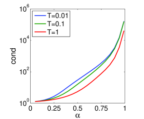
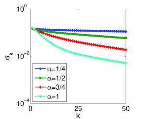
(a) condition number	(b) singular values

Figure 9. Numerical results for the inverse source problem with flux data at $x=0$ and $f(x,t)=xp(t)$, an unknown time dependent component $p(t)$. (a) The condition number of the discrete forward map and (b) singular value spectrum at $T=1$.

It is widely accepted in inverse heat conduction that an inverse problem will be severely ill-posed when the data and unknown are not aligned in the same space/time direction, and only mildly ill-posed when they do align with each other. Our discussions with the inverse source problems indicate that the observation remains valid in the time fractional diffusion case. In particular, although not presented, we note that the inverse source problem of recovering a space dependent component from the lateral Cauchy data is severely ill-posed for both fractional and normal diffusion. In the simplest case of a space dependent only source term, it is mathematically equivalent to unique continuation, a well known example of severely ill-posed inverse problems.

The inverse source problems for the classical diffusion equation have been extensively studied; see e.g., [7, 37, 9]. Inverse source problems for FDEs have also been numerically studied. Zhang and Xu [111] established the unique recovery of a space dependent source term in (3.1) with pure Neumann boundary data and overspecified Dirichlet data at $x=0$. This is achieved by an eigenexpansion and Laplace transform, and the uniqueness follows from a unique continuation principle of analytic functions. Sakamoto and Yamamoto [89] discussed the inverse problem of determining a spatially varying function of the source term by final overdetermined data in multi-dimension, and established its well-posedness in the Hadamard sense except for a discrete set of values of the diffusion constant, using an analytic Fredholm theory. Very recently, Luchko et al [68] showed the uniqueness of recovering a nonlinear source term from the boundary measurement, and developed a numerical scheme of fixed point iteration type. Aleroev et al [2] showed the uniqueness of recovering a space dependent source term from integral type observational data. Recently, there are many numerical studies on this class of inverse problems. In [101], the numerical recovery of a spatially varying function of the source term from the final time data in a general domain was studied using a quasi-boundary value problem method; see also [112, 98] related studies. Wang et al [100] proposed to determine the space-dependent source term from the final time data in multi-dimension using a reproducing kernel Hilbert space method.

3.4. Inverse potential problem

Now we consider a nonlinear inverse coefficient problem for the time fractional diffusion equation: given the final time data $g=u(T)$, find the potential $q$ in the model

(3.5) $$\partial_{t}^{\alpha}u-u_{xx}+qu=0\quad\mbox{ in }\Omega,$$

with a homogeneous Neumann boundary condition and initial data $v$. The parabolic counterpart has been extensively studied [38, 15, 16], where it was shown that the problem is nearly well-posed in the Hardamard sense in suitable Hölder space, under certain conditions, using the strong maximum principle. In [38], an elegant fixed point method was developed, and the monotone convergence of the method was established. It can be adapted straightforwardly to the fractional case: given an initial guess $q^{0}$, compute the update $q^{k}$ recursively by

$$q^{k+1}=\frac{g^{\prime\prime}-\partial_{t}^{\alpha}u(x,T;q^{k})}{g},$$

where the notation $u(x,T;q^{k})$ denote the solution to problem (3.5) with the potential $q^{k}$ at $t=T$. Since the strong maximum principle is still valid for the time fractional diffusion equation [110], the scheme is monotonically convergent, under suitable conditions.

As the terminal time $T\to\infty$, the problem recovers a steady-state problem, and the scheme amounts to twice numerical differentiation in space and converges within one iteration, provided that the data $g$ is accurate enough. Hence, it is natural to expect that the convergence of the scheme will depends crucially on the time $T$: the larger is the time $T$, the closer is the solution $u$ to the steady state solution; and thus the faster is the convergence of the fixed point scheme. By Lemma 2.1, as the fractional order $\alpha$ approaches zero, the solution $u$ decays much faster around $t=0$ than the classical one, i.e., $\alpha=1$. In other words, the fractional diffusion problem can reach a “quasi-steady state” much faster than the classical one, especially for $\alpha$ close to zero, and the scheme will then converge much faster.

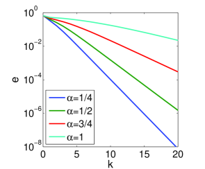
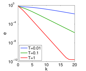
(a) error at $T=0.1$	(b) error at $\alpha=1/2$

Figure 10. Numerical results, i.e., the relative $L^{2}(\Omega)$ error $e$, for the inverse potential problem from exact final time data at (a) $T=0.1$ and (b) $\alpha=1/2$.

To illustrate the point, we present in Fig. 10 some numerical results of reconstructing a discontinuous potential $q=1+2x\chi_{[0,0.5]}+2(1-\chi_{(0.5,1]}x)$ (with $\chi_{S}$ being the characteristic function of the set $S$) from exact data, in order to illustrate the convergence behavior of the fixed point scheme. In the figure, $e$ denotes the relative $L^{2}(\Omega)$ error. The numerical results fully confirm the preceding discussions: at a fixed time $T$, the smaller is the fractional order $\alpha$, the faster is the convergence; and at fixed $\alpha$, the larger is the time $T$, the faster is the convergence. Numerically, one also observes the monotone convergence of the scheme.

Generally, the recovery of a coefficient in FDEs has not been extensively studied. Cheng et al [14] established the unique recovery of the fractional order $\alpha\in(0,1)$ and the diffusion coefficient from the lateral boundary measurements. It represents one of the first mathematical works on invere problems for FDEs, and has inspired many follow-up works. Yamamoto and Zhang [109] established conditional stability in determining a zeroth-order coefficient in a one-dimensional FDE with one half order Caputo derivative by a Carleman estimate. Carleman estimates for time fractional diffusion were discussed in [108, 13, 62]. In [73], the unique determination of the spatial coefficient and/or the fractional order from the data on a subdomain was shown for a positive initial condition. Wang and Wu [97] studied the simultaneous recovery of two time varying coefficients, i.e., a kernel function and a source function, from the additional integral observation in multi-dimension, using a fixed point theorem. All these works are concerned with the theoretical analysis, ant there are even fewer works on the numerical analysis of related inverse problems. Li et al [58] suggested an optimal perturbation algorithm for the simultaneous numerical recovery of the diffusion coefficient and fractional order in a one-dimensional time fractional FDE. In [50], the authors considered the identification of a potential term from the lateral flux data at one fixed time instance corresponding to a complete set of source terms, and established the unique determination for “small” potentials. Further, a Newton type method was proposed in [50], and its convergence was shown.

Even though our discussions have focused on time fractional diffusion, which involves one single fractional derivative in time, it is also possible to consider equations where the time derivative involves multiple factional orders, i.e., $\sum_{k=1}^{m}c_{k}\partial_{t}^{\alpha_{k}}$ for a sequence $\alpha_{1}>\alpha_{2}>\,\ldots>\alpha_{m}$ [60, 44]; see [59] for some first uniqueness results for inverse coefficient problems in the multi-dimensional case. Further extensions include the distributed-order, spatially and/or temporally variable-order and tempered fractional diffusion, to better capture certain physical processes, for which, however, related inverse problems have not been discussed at all.

3.5. Fractional derivative as an inverse solution

One of the very first undetermined coefficient problems for PDEs was discussed in the paper by B. Frank Jones Jr. [52] (see also [8, Chapter 13]). This is to determine the coefficient $a(t)$ from

$$u_{t} =a(t)u_{xx},\quad 0<x<\infty,\quad t>0$$

$$u(x,0) =0,\quad-a(t)u_{x}(0,t)=g(t),\quad 0<t<T$$

under the over-posed condition of measuring the “temperature” at $x=0$

$$u(0,t)=\psi(t)$$

In [52], B. Frank Jones Jr. provided a complete analysis of the problem, by giving necessary and sufficient conditions for a unique solution as well as determining the exact level of ill-conditioning. The key step in the analysis is a change of variables and conversion of the problem to an equivalent integral equation formulation. Perhaps surprisingly, this approach involves the use of a fractional derivative as we now show.

The assumptions are that $g$ is continuous and positive and $\psi$ is continuously differentiable with $\psi(0)=0$ and $\psi^{\prime}>0$ on $(0,T)$. In addition, the function $h(t)$ defined by

$$h(t)=\frac{\sqrt{\pi}g(t)}{\int_{0}^{t}(t-\tau)^{-1/2}\psi^{\prime}(\tau)d\tau}$$

satisfies $\lim_{t\to 0}h(t)=h_{0}>0$. Note that $h$ is the ratio of the two data functions; the flux $g$ and the Djrbashian-Caputo derivative of order $1/2$ of $\psi$. If we define $h_{i}=\inf h$ and $h_{s}=\sup h$ on $[0,T]$ and look at the space $\mathcal{G}:=\{a\in C[0,T):h_{i}^{2}\leq a(t)\leq h_{s}^{2}\}$, then it was shown that any $a\in\mathcal{G}$ satisfies the inverse problem must also solve the integral equation

$$a(t)=\frac{\sqrt{\pi}g(t)}{\int_{0}^{t}\psi^{\prime}(\tau)[\int_{\tau}^{t}a(s)\,ds]^{-1/2}d\tau}=:\mathcal{T}a,$$

and vice-versa. The main result in [52] is that the operator $\mathcal{T}$ has a unique fixed point on $\mathcal{G}$ and indeed $\mathcal{T}$ is monotone in the sense of preserving the partial order on $\mathcal{G}$, i.e., if $a_{1}\geq a_{2}$ then $\mathcal{T}a_{1}\leq\mathcal{T}a_{2}$.

Given these developments, it might seem that a parallel construction for the time fractional diffusion counterpart, $\partial_{t}^{\alpha}u=a(t)u_{xx}$, would be relatively straightforward but this seems not to be the case. The basic steps for the parabolic version require items that just are not true in the fractional case, such as the product rule, and without these the above structure cannot be replicated or at least not without some further ingenuity.

4. Inverse problems for space fractional diffusion

Now we turn to differential equations involving a fractional derivative in space. There are several possible choices of a fractional derivative in space, e.g., Djrbashian-Caputo fractional derivative, Riemann-Liouville fractional derivative, Riesz derivative, and fractional Laplacian [3], which all have received considerable attention. In recent years, the use of the fractional Laplacian is especially popular in high-dimensional spaces, and admits a well-developed analytical theory. We shall focus on the left-sided Djrbashian-Caputo fractional derivative $\,{}_{0}^{C}\kern-1.99997ptD^{\beta}_{\kern-0.70004ptx}$, $\beta\in(1,2)$, and the one-dimensional case, and consider the following four inverse problems: inverse Sturm-Liouville problem, Cauchy problem for a fractional elliptic equation, backwards diffusion, and sideways problem.

4.1. Inverse Sturm-Liouville problem

First we consider the following Sturm-Liouville problem on the unit interval $\Omega=(0,1)$: find $u\in H_{0}^{1}(\Omega)\cap H^{\beta}(\Omega)$ and $\lambda\in\mathbb{C}$ such that

(4.1) $$-\,_{0}^{C}\kern-1.99997ptD^{\beta}_{\kern-0.70004ptx}u+qu=\lambda u\quad\mbox{in }\Omega,$$

with a homogeneous Dirichlet boundary condition $u(0)=u(1)=0$. A Sturm-Liouville problem of this form was considered by Mkhitar M Djrbashian [22, 19] in 1960s to construct certain biorthogonal basis for spaces of analytic functions; see also [78]. Like before, with $\beta=2$, it recovers the classical Sturm-Liouville problem. In the case of a general potential $q$, in the fractional case, little is known about the analytical properties of the eigenvalues and eigenfunctions. For the case of a zero potential $q=0$, there are countably many eigenvalues $\{\lambda_{j}\}$ to (4.1), which are zeros of the Mittag-Leffler function $E_{\beta,2}(-\lambda)$. The corresponding eigenfunctions are given by $xE_{\beta,2}(-\lambda_{j}x^{\beta})$. Using the exponential asymptotics on the Mittag-Leffler function in Lemma 2.1, one [93, 50] can show that asymptotically, the eigenvalues $\lambda_{j}$ are distributed as

$$|\lambda_{j}|\sim(2\pi j)^{\beta}\quad\mbox{and}\quad\mathrm{arg}(\lambda_{j})\sim\frac{(2-\beta)\pi}{2}.$$

Hence, for any $\beta\in(1,2)$, there are only a finite number of real eigenvalues to (4.1), and the rest appears as complex conjugate pairs.

It is well known that eigenvalues contain valuable information about the boundary value problem. For example it is known that the sequence of Dirichlet eigenvalues can uniquely determine a potential $q$ symmetric with respect to the point $x=1/2$, and together with additional spectral information, one can uniquely determine a general potential $q$; see [12, 86] for an overview of results on the classical inverse Sturm-Liouville problem. In the fractional case, the eigenvalues are generally genuinely complex, and a complex number may carry more information than a real one. Thus one naturally wonders whether these complex eigenvalues do contain more information about the potential. Numerically the answer is affirmative. To illustrate this, we show some numerical reconstructions in Fig. 11, obtained by using a frozen Newton method and representing the sought-for potential $q$ in Fourier series [50]. The Dirichlet eigenvalues can be computed efficiently using a Galerkin finite element method [45]. One observes that one single Dirichlet spectrum can uniquely determine a general potential $q$. Unsurprisingly, as the fractional order $\beta$ tends two, the reconstruction becomes less and less accurate, since in the limit $\beta=2$, the Dirichlet spectrum cannot uniquely determine a general potential $q$. Theoretically, the surprising uniqueness in the fractional case remains to be established.

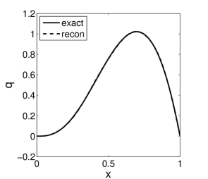
(a) $\beta=5/3$	(b) $\beta=7/4$

Figure 11. Numerical results for the inverse Sturm-Liouville problem with a Djrbashian-Caputo derivative for (a) $\beta=5/3$ and (b) $\beta=7/4$. The reconstructions are computed from the first eight eigenvalues (in absolute value) using a frozen Newton method [50].

Naturally, one can also consider the Riemann-Liouville case:

(4.2) $$-{{}_{0}^{\kern-0.70004ptR}\kern-1.99997ptD^{\beta}_{\kern-0.70004ptx}u}+qu=\lambda u\quad\mbox{ in }\Omega,$$

with $u(0)=u(1)=0$. Like before, little is known about the analytical properties of the eigenvalues and eigenfunctions. In the case of a zero potential $q=0$, there are countably many eigenvalues to (4.2), which are zeros of the Mittag-Leffler function $E_{\beta,\beta}(-\lambda)$, and the corresponding eigenfunctions are given by $x^{\beta-1}E_{\beta,\beta}(-\lambda_{j}x^{\beta})$. Further, the asymptotics of the eigenvalues are still valid. Hence, for any $\beta\in(1,2)$, there are only a finite number of real eigenvalues to (4.2), and the rest appears as complex conjugate pairs.

The numerical results from the Dirichlet spectrum in the Riemann-Liouville case are shown in Fig. 12. For a general potential $q$, the reconstruction represents only the symmetric part, which is drastically different from the Djrbashian-Caputo case, but identical with that for the classical Sturm-Liouville problem. Further, if we assume that the potential $q$ is known on the left half interval, then the Dirichlet spectrum allows uniquely reconstructing the potential $q$ on the remaining half interval, cf., Fig. 12(b). These results indicate that in the Riemann-Liouville case the complex spectrum is not more informative than the classical Sturm-Liouville problem. The precise mechanism underlying the fundamental differences between the Djrbashian-Caputo and Riemann-Liouville cases awaits further study. However, as in the classical case $\beta=2$, one can show that the linearized derivative of the map $q\to u(1;\lambda,q)$ around $q=0$ cannot span more than the subspace of even functions in $L^{2}(\Omega)$.

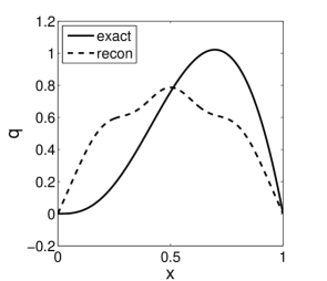
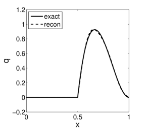
(a) whole interval	(b) half interval

Figure 12. Numerical results for the inverse Sturm-Liouville problem with a Riemann-Liouville fractional derivative of order $\beta=4/3$. The reconstructions are computed from the first eight eigenvalues (in absolute value) using a frozen Newton method [50].

In general, the Sturm-Liouville problem with a fractional derivative remains completely elusive, and numerical methods such as finite element method [46] provide a valuable (and often the only) tool for studying its analytical properties. For a variant of the fractional Sturm-Liouville problem, which contains a fractional derivative in the lower-order term, Malamud [71] established the existence of a similarity transformation, analogous to the well-known Gel’fand-Levitan-Marchenko transformation, and also the unique recovery of the potential from multiple spectra. In the classical case, the Gel’fand-Levitan-Marchenko transformation lends itself to a constructive algorithm [86]; however, it is unclear whether this is true in the fractional case. In [50], the authors proposed a Newton type method for reconstructing the potential, which numerically exhibits very good convergence behavior. However, a rigorous convergence analysis of the scheme is still missing. Further, the uniqueness and nonuniqueness issues of related inverse Sturm-Liouville problems are outstanding. Last, as noted above, there are other possible choices of the space fractional derivative, e.g., fractional Laplacian and Riesz derivative. It is unknown whether the preceding observations are valid for these alternative derivatives.

4.2. Cauchy problem for fractional elliptic equation

One classical elliptic inverse problem is the Cauchy problem for the Laplace equation, which plays a fundamental role in the study of many elliptic inverse problems [40]. A first example was given by Jacques Hadamard [31] to illustrate the severe ill-posedness of the Cauchy problem, which motivated him to introduce the concept of well-posedness and ill-posedness for problems in mathematical physics. So a natural question is whether the Cauchy problem for the fractional elliptic equation is also as ill-posed? To illustrate this, we consider the following fractional elliptic problem on the rectangular domain $\Omega=\{(x,y)\in\mathbb{R}^{2}:0<x<1,0<y<1\}$

(4.3) $${\,{}_{0}^{C}\kern-1.99997ptD^{\beta}_{\kern-0.70004ptx}}u+{\,{}_{0}^{C}\kern-1.99997ptD^{\beta}_{\kern-0.70004pty}}u=0\mbox{ in }\Omega,$$

with the fractional order $\beta\in(1,2)$ and the Cauchy data

$$u(x,0)=g(x)\quad\mbox{and}\quad\frac{\partial u}{\partial\nu}(x,0)=h(x),\ \ 0<x<1$$

where $\nu$ is the unit outward normal direction. With $\beta=2$, it recovers the Cauchy problem for the Laplace equation. By applying the separation of variables, we assume that $u(x,y)=\phi(x)\psi(y)$, which directly gives for some scalar $\lambda\in\mathbb{C}$ that

$${\,{}_{0}^{C}\kern-1.99997ptD^{\beta}_{\kern-0.70004ptx}}\phi(x) =-\lambda\phi(x),$$

$${\,{}_{0}^{C}\kern-1.99997ptD^{\beta}_{\kern-0.70004pty}}\psi(y) =\lambda\psi(y),$$

Let $(\lambda_{j},\phi_{j})$ be a Dirichlet eigenpair of the Caputo derivative operator $-{\,{}_{0}^{C}\kern-1.99997ptD^{\beta}_{\kern-0.70004ptx}}$ on the unit interval $D=(0,1)$, i.e., $\phi_{j}(x)=xE_{\beta,2}(-\lambda_{j}x^{\beta})$, and $|\lambda_{j}|\to\infty$ as $j\to\infty$ [51]; see Section 4.1 for further details. With the choice $\phi=\phi_{j}$ and the Cauchy data pair $(g,h_{j})=(0,-xE_{\beta,2}(\lambda_{j}x^{\beta})/\lambda_{j})$, the component $\psi_{j}$ satisfies

$${\,{}_{0}^{C}\kern-1.99997ptD^{\beta}_{\kern-0.70004pty}}\psi_{j}(y)=\lambda_{j}\psi_{j}(y)\mbox{ in }y\in(0,\infty),$$

with the initial condition $\psi_{j}(0)=0$ and $\frac{d}{dy}\psi_{j}(0)=1/\lambda_{j}$. Using the relation $\frac{d}{dx}x^{\gamma-1}E_{\beta,\gamma}(\lambda x^{\beta})=\lambda x^{\gamma-2}E_{\beta,\gamma-1}(\lambda x^{\beta})$ [53, pp. 46], we deduce that the solution $\psi_{j}$ to the fractional ordinary differential equation is given by

$$\psi_{j}(y)=yE_{\beta,2}(\lambda_{j}y^{\beta})/\lambda_{j}.$$

Hence, $u_{j}(x,y)=xE_{\beta,2}(-\lambda_{j}x^{\beta})yE_{\beta,2}(\lambda_{j}y^{\beta})/\lambda_{j}^{2}$ is a solution to the Cauchy problem with $g=0$ and $h_{j}(x)=-xE_{\beta,2}(-\lambda_{j}x^{\beta})/\lambda_{j}$. By the exponential asymptotics of the Mittag-Leffler function, cf. Lemma 2.1, we deduce that $h_{j}(x)\to 0$ as $j\to\infty$, whereas for any $y>0$, the solution $u_{j}(x,y)\to\infty$ as $j\to\infty$, in view of the exponential growth of the Mittag-Leffler function $E_{\beta,2}(z)$, cf. Lemma 2.1. This indicates that the Cauchy problem for the fractional elliptic equation is also exponentially ill-posed. However, the interesting question of the degree of ill-posedness, in comparison with the classical case, is unclear and certainly worthy of further study. Further, we note that the numerical solution of the fractional elliptic equation (4.3) is highly nontrivial, and there seems no efficient yet rigorous solver available in the literature, due to a lack of solution theory for such problems.

4.3. Backward problem

Now we return to the backward diffusion problem with fractional derivatives in the space variable(s). Let $\Omega=(0,1)$ be the unit interval. Then the one-dimensional space fractional diffusion equation is given by

$$u_{t}-{\,{}_{0}^{C}\kern-1.99997ptD^{\beta}_{\kern-0.70004ptx}}u=0,\quad(x,t)\in\Omega\times(0,\infty),$$

where the fractional order $\beta\in(1,2)$. The equation is equipped with the following initial condition $u(x,0)=v$ and zero boundary condition $u(0,t)=u(1,t)=0$. The backward problem is: given the final time data $g(x)=u(x,T)$, find the initial data $v$. Since the Djrbashian-Caputo derivative operator $\,{}_{0}^{C}\kern-1.99997ptD^{\beta}_{\kern-0.70004ptx}$ with the zero Dirichlet boundary is sectorial on suitable spaces [42], the existence of a solution $u$ follows from the analytic semigroup theory [81, 43], and formally it can be represented by

$$u(t)=e^{-At}v,$$

where $A$ is the representation of the Djrbashian-Caputo derivative operator $-\,_{0}^{C}\kern-1.99997ptD^{\beta}_{\kern-0.70004ptx}$ on its domain. Formally, the solution $v$ to the space fractional backward problem is given by

$$v=e^{AT}g.$$

In case of $\beta=2$, using the eigenpairs $\{(\lambda_{j},\phi_{j})\}$ and the $L^{2}(\Omega)$ orthogonality of the eigenfunctions $\{\phi_{j}\}$, it recovers the well known formula

$$v=\sum_{j=1}^{\infty}e^{\lambda_{j}T}(g,\phi_{j})\phi_{j}.$$

The growth factor $e^{\lambda_{j}T}$ explains the severely ill-posed nature of the inverse problem. In the fractional case, such an explicit representation is no longer available since the corresponding eigenfunctions $\{\phi_{j}\}$ are not orthogonal in $L^{2}(\Omega)$ (actually they can be almost linearly dependent), due to the non self adjoint nature of the Djrbashian-Caputo derivative operator $-\,_{0}^{C}\kern-1.99997ptD^{\beta}_{\kern-0.70004ptx}$. Nonetheless, according to the discussions in Section 4.1, the eigenvalues $\{\lambda_{j}\}$ increase to infinity with the index $j$, and asymptotically lies on two rays. Hence, one naturally expects that the backward problem is also exponentially ill-posed. However, the magnitudes (and the real parts) of the eigenvalues grow at a rate slower than that of the standard Sturm-Liouville problem, and thus the space fractional backward problem is less ill-posed than the classical one. To illustrate the point, we present the numerical results in Fig. 13. For all fractional orders $\beta$, the singular values decay exponentially, but the decay rate increases dramatically with the increase of the fractional order $\beta$ and the terminal time $T$. Hence, anomalous superdiffusion does not change the exponentially ill-posed nature of the backward problem, but numerically it does enable recovering more Fourier modes of the initial data $v$.

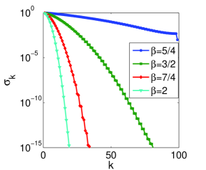
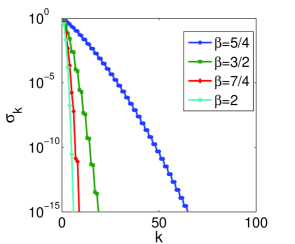
(a) $T=0.01$	(b) $T=0.1$

Figure 13. Numerical results for the space fractional backward diffusion problem, the singular value spectrum at two different time instances, (a) $T=0.01$ and (b) $T=0.1$.

Last, we note that for other choices of the fractional derivative, e.g., the Riemann-Liouville fractional derivative and the fractional Laplacian [6, 55], the magnitude of eigenvalues of the operator also tends to infinity, and the growth rate increases with the fractional order $\beta$. Therefore, the preceding observations on the space fractional backward problem are expected to be valid for these choices as well.

4.4. Sideways problem

Last we return to the classical sideways diffusion problem but now with a fractional derivative in space rather than in time. Let $\Omega=(0,1)$ be the unit interval. Then the one-dimensional space fractional diffusion equation is given by

$$u_{t}-{\,{}_{0}^{C}\kern-1.99997ptD^{\beta}_{\kern-0.70004ptx}}u=0,\quad(x,t)\in\Omega\times(0,\infty),$$

where the fractional order $\beta\in(1,2)$. The equation is equipped with an initial condition $u(x,0)=0$ and the following lateral Cauchy boundary conditions

$$u(0,t)=f(t)\ \quad\mbox{and}\quad\ u_{x}(0,t)=g(t),\ \ t>0.$$

We wish to compute the solution at $x=1$, i.e., $h(t):=u(1,t)$. In the case $\beta=2$, the model recovers the standard diffusion equation, and we have already discussed the severe ill-conditioning of the classical case. Due to the nonlocal nature of the fractional derivative, one might expect that in the space fractional case, the sideways problem is less ill-posed. To see this, we take Laplace transform in time to arrive at (with $\ \widehat{}\$ denoting the Laplace transform)

$$z\widehat{u}(x,z)-{\,{}_{0}^{C}\kern-1.99997ptD^{\beta}_{\kern-0.70004ptx}}\widehat{u}(x,z)=0,$$

with the initial conditions (at $x=0$)

$$\widehat{u}(0,z)=\widehat{f}(z)\quad\mbox{and}\quad\widehat{u}_{x}(0,z)=\widehat{g}(z).$$

The solution $\widehat{u}(x,z)$ to the initial value problem is given by

$$\widehat{u}(x,z)=\widehat{f}(z)E_{\beta,1}(zx^{\beta})+\widehat{g}(z)xE_{\beta,2}(zx^{\beta})$$

and thus

$$\widehat{h}(z)=\widehat{f}(z)E_{\beta,1}(z)+\widehat{g}(z)E_{\beta,2}(z).$$

Like before, the boundary condition $h(t)$ at $x=1$ can be found by an inverse Laplace transform

$$h(t)=\int_{Br}e^{zt}\widehat{h}(z)dz.$$

In case of $\beta=2$, this gives $\cosh\sqrt{z}$ and $\sinh\sqrt{z}/\sqrt{z}$ multipliers to the data $\widehat{f}(z)$ and $\widehat{g}(z)$ resulting in the exponential ill-conditioning of the sideways heat problem. In the case of a general $\beta\in(1,2)$, the exponential asymptotics in Lemma 2.1 indicates that the problem still suffers from exponentially growing multipliers to the data, and thus the problem is still severely ill-conditioned. Simple computation shows that the multiplier is asymptotically larger for the fractional order $\beta$ closer to unity. In other words, anomalous diffusion in space does not mitigate the ill-conditioned nature of the sideways problem, but actually worsens the conditioning severely.

To further illustrate the point, we compute the forward map $F$ from the Dirichlet boundary condition at $x=1$ to the flux at $x=0$ numerically with a finite element in space/finite difference in time scheme, cf. Appendix A.3 for the details. The numerical results are presented in Fig. 14. The singular value spectra clearly show the ill-posedness nature of the space fractional sideways problem: as the fractional order $\beta$ increases from one to two, the majority of the singular values move upward, the decay of the singular values slows down, and thus the sideways problem becomes less and less ill-posed (but still severely so). Further, there are more tiny singular values kicking in as the fractional order $\beta$ decreases to one, which indicates the inherent rank deficiency of the forward map $F$ and might be relevant in the uniqueness of the inverse problem. This confirms the preceding analysis: the degree of ill-posedness worsens with the decrease of the fractional order $\beta$, and the fractional counterpart is more ill-posed than the classical one. In other words, anomalous diffusion actually severely worsens the conditioning of the already very ill-posed sideways problem. Further, the numerical results tend to indicate that the Djrbashian-Caputo derivative with an order $\beta\in(1,2)$ acts as an interpolation between the diffusion and convection, which results in a history mechanism in space: when the history piece runs from the left to the right, it is unlikely to propagate the information in the reverse direction; and the closer is the fractional order $\beta$ to unity, the stronger is the directional effect. The latter is not counterintuitive, since in the limit of $\beta=1$, the Djrbashian-Caputo fractional derivative $\,{}_{0}^{C}\kern-1.99997ptD^{\beta}_{\kern-0.70004ptx}u$ recovers the first order derivative $\frac{\partial u}{\partial x}$, and the problem is of convection type, and surely no information can be convected backwards!

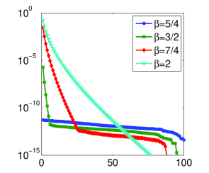
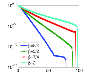
(a) $T=0.1$	(b) $T=1$

Figure 14. Singular value spectrum of the forward map $F$ at times $T=0.1$ and $T=1$, for the sideways problem with Cauchy data at $x=0$.

In the case $\beta=2$, one may equally measure the lateral Cauchy data at $x=1$, and aims at recovering the Dirichlet boundary condition at $x=0$. Clearly, this does not change the nature of the inverse problem, and it is equally ill-posed. Due to the directional nature of the Djrbashian-Caputo derivative $\,{}_{0}^{C}\kern-1.99997ptD^{\beta}_{\kern-0.70004ptx}$, one naturally wonders whether this “directional” feature does influence the ill-posed nature of the sideways problem. To illustrate the point, we repeat the preceding arguments and deduce

$$z\widehat{u}(x,z)-{\,{}_{0}^{C}\kern-1.99997ptD^{\beta}_{\kern-0.70004ptx}}\widehat{u}(x,z)=0,$$

with the boundary conditions at $x=1$

$$\widehat{u}(1,z)=\widehat{f}(z)\quad\mbox{and}\quad\widehat{u}_{x}(1,z)=\widehat{g}(z).$$

To derive the solution, denote the initial conditions at $x=0$ by $\tilde{f}(z)=\widehat{u}(0,z)$ and $\tilde{g}(z)=\widehat{u}_{x}(0,z)$. Then the solution $\widehat{u}(x,z)$ to the initial value problem is given by

$$\widehat{u}(x,z)=\tilde{f}(z)E_{\beta,1}(zx^{\beta})+\tilde{g}xE_{\beta,2}(zx^{\beta}).$$

Use the differentiation formula $\frac{d}{dx}x^{\gamma-1}E_{\beta,\gamma}(zx^{\beta})=zx^{\gamma-2}E_{\beta,\gamma-1}(zx^{\beta})$ [53, page 46], we deduce that at $x=1$, there hold

$$\tilde{f}(z)E_{\beta,1}(z)+\tilde{g}E_{\beta,2}(z) =\widehat{f}(z),$$

$$\tilde{f}(z)E_{\beta,0}(z)+\tilde{g}E_{\beta,1}(z) =z^{-1}\widehat{g}(z).$$

Solving the linear system yields the solution to the sideways problem

$$\tilde{f}(z)=\frac{E_{\beta,1}(z)\widehat{f}(z)-z^{-1}E_{\beta,2}(z)\widehat{g}(z)}{E_{\beta,1}(z)^{2}-E_{\beta,0}(z)E_{\beta,2}(z)},$$

and accordingly the solution $h(t)\equiv u(0,t)$ is given by an inverse Laplace transform. The growth factors of the data $\widehat{f}$ and $\widehat{g}$ are $E_{\beta,1}(z)/(E_{\beta,1}(z)^{2}-E_{\beta,0}(z)E_{\beta,2}(z))$ and $z^{-1}E_{\beta,2}(z)/(E_{\beta,1}(z)^{2}-E_{\beta,0}(z)E_{\beta,2}(z))$, respectively. The growth of these factors at large $z$ argument determines the degree of ill-conditioning of the sideways problem. To this end, we appeal to the exponential asymptotic of the Mittag-Leffler function $E_{\alpha,\beta}(z)$, cf. Lemma 2.1, and note that Bromwhich path lies in the sector $|\arg z|\leq\pi/2$ to deduce that for large $|z|$, there holds

$$E_{\beta,1}(z)^{2} \sim\frac{1}{\beta^{2}}e^{2z^{1/\beta}}-\frac{2}{\beta\Gamma(1-\beta)z}e^{z^{1/\beta}},$$

$$E_{\beta,0}(z)E_{\beta,2}(z) \sim\frac{1}{\beta^{2}}e^{2z^{1/\beta}}-\frac{1}{\beta\Gamma(2-\beta)}z^{1/\beta-1}e^{z^{1/\beta}}.$$

Hence, the numerator $E_{\beta,1}(z)^{2}-E_{\beta,0}(z)E_{\beta,2}(z)$ behaves like

$$E_{\beta,1}(z)^{2}-E_{\beta,0}(z)E_{\beta,2}(z)\sim\frac{1}{\beta\Gamma(2-\beta)}z^{1/\beta-1}e^{z^{1/\beta}}\qquad\mbox{as }|z|\to\infty.$$

This together with the exponential asymptotic of $E_{\beta,1}(z)$ and $E_{\beta,2}(z)$ from Lemma 2.1 indicates that the multipliers for $\widehat{f}$ and $\widehat{g}$ are growing at most at a very low-order polynomial rate, for large $z$. Hence, the high-frequency components of the data noise are not amplified much (at most polynomially instead of exponentially). The analysis indicates that the sideways problem with the lateral Cauchy data specified at the point $x=1$ is nearly well-posed, as long as the fractional order $\beta$ is away from two, for which it recovers the classical ill-posed sideways problem for the heat equation.

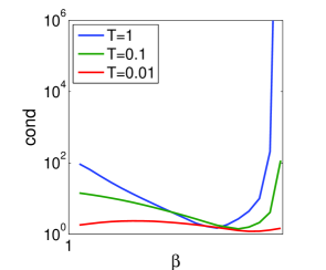
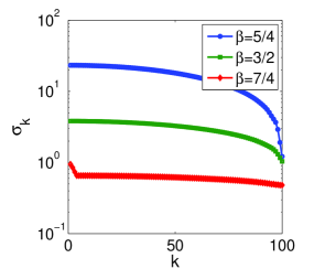
(a) condition number	(b) $T=1$

Figure 15. Numerical results for the space fractional sideways problem, with the lateral Cauchy data at the point $x=1$: (a) the condition number v.s. the fractional order $\beta$ and (b) the singular value spectrum at $T=1$.

Next we illustrate the preceding discussions numerically. The behavior of the forward map $F$ from the Dirichlet boundary at $x=0$ to the flux data at $x=1$ is shown in Fig. 15. For a wide range of values of the fractional order $\beta$, the condition number of the forward map $F$ is of order $100$, which is fairly mild, in view of the size of the linear system, i.e., $100\times 100$. When the fractional order $\beta$ increases towards two, the inverse problem recovers the classical sideways problem, and as expected, the condition number increases dramatically. However, the onset of the blowup depends on the terminal time $T$: the smaller is the time $T$, the smaller seems the onset value. The precise mechanism for this phenomenon is still unknown. For $\beta\leq 7/4$, the singular value spectrum only spans a narrow interval, resulting in a very small condition number. Physically, like before, this can be explained as the “convective” nature of the Djrbashian-Caputo fractional derivative: as the fractional order $\beta$ tends to unity, the information at $x=0$ is transported to $x=1$, free from distortion, and thus the inverse problem is almost well-posed. In summary, depending on the location of the over-specified data, anomalous superdiffusion can either help or aggravate the conditioning of the sideways problem.

Last, we would like to note that the study of space fractional inverse problems, either theoretical or numerical, is fairly scarce. This is partly attributed to the relatively poor understanding of forward problems for FDEs with a space fractional derivative: There are only a few mathematical studies on one-dimensional space fractional diffusion, and no mathematical study on multi-dimensional problems involving space fractional derivatives (of either Riemann-Liouville or Caputo type). Nonetheless, our preliminary numerical experiments show distinct new features for related inverse problems, which motivate their analytical studies.

5. Concluding remarks

Anomalous diffusion processes arise in many disciplines, and the physics behind is very different from normal diffusion. The unusual physics greatly influences the behavior of related forward problems. Further, it is well known that backward fractional diffusion is much less ill-posed than the classical backward diffusion, which has contributed to the belief that inverse problems for anomalous diffusion are always better behaved than that for the normal diffusion. In this work we have examined several exemplary inverse problems for anomalous diffusion processes in a numerical and semi-analytical manner. These include the sideways problem, backward problem, inverse source problem, inverse Sturm-Liouville problem and Cauchy problems. Our findings indicate that anomalous diffusion can give rise to very unusual new features, but they only partially confirm the belief: depending on the data and unknown, it may influence either positively or negatively the degree of ill-posedness of the inverse problem.

The mathematical study of inverse problems in anomalous diffusion is still in its infancy. There are only a few rigorous theoretical results on the uniqueness, existence and stability, which mostly focus on the one-dimensional case, and there are many more open problems awaiting investigations. The development of stable and efficient reconstruction procedures is an active ongoing research topic. However, due to the nonlocality of the forward model, the construction of efficient schemes and their rigorous numerical analysis remain very challenging. This is especially true for space fractional FDEs, and there are almost no theoretical or rigorous numerical studies.

Appendix A Numerical methods for special functions and FDEs

A.1. Computation of the Mittag-Leffler and Wright functions

Like many special functions, the efficient and accurate numerical computation of the Mittag-Leffler function $E_{\alpha,\beta}(z)$ is delicate [28, 29, 94]. An efficient algorithm relies on partitioning the complex plane $\mathbb{C}$ into different regions, where different approximations, i.e., power series, integral representation and exponential asymptotic for small values of the argument, intermediate values and large values, respectively, are used for efficient numerical computation; see [94] for the some partition and error estimates. The special case of the Mittag-Leffler function $E_{\alpha,\beta}(z)$ with a real argument $z\in\mathbb{R}$, which plays a predominant role in time-fractional diffusion, can also be efficiently computed with the Laplace transform and suitable quadrature rules [27].

The computation of the Wright function $W_{\rho,\mu}(z)$ is even more delicate. In theory, like before, it can be computed using power series for small values of the argument and a known asymptotic formula for large values, and for the intermediate case, values are obtained by using an integral representation [67]. The integral representation for the Wright function $W_{\rho,\mu}(z)$ for intermediate values in the case of interest for the fundamental solution in one-dimension (where $\rho=-\alpha/2<0$, $0<\mu=1+\rho<1$ and $z=-x$, $x>0$) is given by

$$W_{\rho,\mu}(-x)=\int_{0}^{\infty}K(x,\rho,\mu,r)\,dr\qquad$$

where the kernel $K(x,\rho,\mu,r)$ is given by

$$K(x,\rho,\mu,r)=r^{-\mu}e^{-r+x\cos(\pi\rho)r^{-\rho}}\sin(x\sin(\pi\rho)r^{-\rho}+\pi\mu).$$

This is a singular kernel with a leading order $r^{-\mu}=r^{-1-\rho}$, with successive singular kernels of the form $r^{-1-2\rho}$, $r^{-1-3\rho}$ etc., upon expanding the terms. Hence, a direct treatment via numerical quadrature is inefficient. A more efficient approach is to use the change of variable $s=r^{-\rho}$, i.e., $r=s^{-1/\rho}$, and the transformed kernel is

$$\widetilde{K}(x,\rho,\mu,s)=(-\rho)^{-1}s^{(-\rho)^{-1}(-\mu+1)-1}e^{-s^{-\frac{1}{\rho}}+x\cos(\pi\rho)s}\sin(x\sin(\pi\rho)s+\pi\mu).$$

The fundamental solution of the one-dimensional time-fractional diffusion equation is expressed in terms of a Wright function $W_{\rho,\mu}(-x)$ with the choice $\rho=-\alpha/2$ and $\mu=1+\rho$, cf. (2.2). In this case the resulting kernel $\tilde{K}$ simplifies to

$$\widetilde{K}(x,\rho,1+\rho,s)=(-\rho)^{-1}e^{-s^{-\frac{1}{\rho}}+x\cos(\pi\rho)s}\sin(x\sin(\pi\rho)s+(1+\rho)\pi).$$

This kernel is free from the grave singularity, and thus the quadrature method is quite effective. In general, the integral can be computed efficiently via the Gauss-Jacobi quadrature, with the weight function $s^{(-\rho)^{-1}(-\mu+1)-1}$. We note that an algorithm for the Wright function $W_{\rho,\mu}(z)$ over the whole complex plane $\mathbb{C}$ with rigorous error analysis is still missing. The endeavor in this direction would almost certainly involve dividing the complex domain $\mathbb{C}$ into different regions, and using different approximations on each region separately.

A.2. Time fractional diffusion

We describe a finite difference method for the initial boundary value problem for the one-dimensional time-fractional diffusion equation

$$\partial_{t}^{\alpha}u-u_{xx}+qu=f(x,t)\quad(x,t)\in\Omega\times(0,T),$$

with the initial condition $u(x,0)=v$ and boundary conditions

$$u(0,t)=g(t)\quad\mbox{and}\quad u(1,t)=h(t),\quad t>0.$$

There are many efficient numerical schemes for discretizing the problem. The discretization in space can be achieved by the standard central difference scheme, Galerkin finite element method [47] or spectral method, and the discretization in time can be achieved with the L1 approximation [96, 63] and convolution quadrature [48]. We shall adopt the L1 approximation in time and the central difference in space. Specifically, we divide the interval $[0,T]$ into uniform subintervals, with nodes $t_{k}=k\tau$, $k=0,\ldots,K$, and a time step size $\tau=T/K$. Similarly, we partition the spatial domain $\Omega$ into uniform subintervals, with grid points $x_{i}=ih$, $i=0,\ldots,N$, and mesh size $h=1/N$. Then the L1-approximation of the Djrbashian-Caputo fractional derivative $\partial_{t}^{\alpha}u(x,t_{k})$ developed in [96, 63] is given by:

(A.1) $$\partial_{t}^{\alpha}u(x,t_{k}) \approx\tau^{-\alpha}\left[b_{0}u(x,t_{k})-b_{k-1}u(x,t_{0})+\sum_{j=1}^{k-1}(b_{j}-b_{j-1})u(x,t_{k-j})\right]$$

where the weights $b_{j}$ are given by

$$b_{j}=((j+1)^{1-\alpha}-j^{1-\alpha})/\Gamma(2-\alpha),\ j=0,1,\ldots,K-1.$$

If the solution $u(x,t)$ is $C^{2}$ continuous in time, the local truncation error of the L1 approximation is bounded by $c\tau^{2-\alpha}$ for some $c$ depending only on $u$ [63, equation (3.3)]. In general, one can show that the scheme is only first-order accurate. Next with the central difference scheme in space and the notation $u_{i}^{k}\approx u(x_{i},t_{k})$, we arrive at the following fully discrete scheme

$$\left[b_{0}u_{i}^{k}-b_{k-1}u_{i}^{0}+\sum_{j=1}^{k-1}(b_{j}-b_{j-1})u_{i}^{k-j}\right]+\frac{u_{i-1}^{k}-2u_{i}^{k}+u_{i+1}^{k}}{h^{2}}+q_{i}u_{i}^{k}=f_{i}^{k},\ \ i=1,\ldots,N-1,$$

with $q_{i}=q(x_{i})$ and $f_{i}^{k}=f(x_{i},t_{k})$. We note that at each time step, one needs to solve a tridiagonal linear system. However, the right hand side at the current step involves all previous steps, which can be quite expensive for a small step size, and this will most likely be required due to the first order in time convergence. This history piece represents one of the main computational challenges for time fractional differential equations. There are high-order schemes, e.g., convolution quadrature generated by the second-order backward difference formula [48]. Further, we note that the finite difference scheme in space can be replaced with the Galerkin finite element method, which is especially suitable for high dimensional problems on a general domain and elliptic operator involving variable coefficients [47].

A.3. Space fractional diffusion

Now we describe a fully discrete scheme based on the backward Euler method in time and a Galerkin finite element method in space for the space fractional diffusion problem on the unit interval $\Omega=(0,1)$

$$u_{t}-{\,{}_{0}^{C}\kern-1.99997ptD^{\beta}_{\kern-0.70004ptx}}u+qu=f\quad\mbox{ in }\Omega\times(0,T],$$

with the initial condition $u=v$ and the Dirichlet boundary condition

$$u(0,t)=g(t)\quad\mbox{and}\quad u(1,t)=h(t),\ \ t>0.$$

The Galerkin finite element method relies on the variational formulation for the fractional elliptic problem

$$-{\,{}_{0}^{C}\kern-1.99997ptD^{\beta}_{\kern-0.70004ptx}}u+qu=f\quad\mbox{ in }\Omega,$$

with a homogeneous Dirichlet boundary condition $u(0)=u(1)=0$, recently developed in [45]. The variational formulation of the problem is given by: find $u\in U\equiv H_{0}^{\beta/2}(\Omega)$ such that

$$-({{}_{0}^{\kern-0.70004ptR}\kern-1.99997ptD^{\beta/2}_{\kern-0.70004ptx}}u,\ _{x}^{\kern-0.70004ptR}\kern-1.99997ptD^{\beta/2}_{\kern-0.70004pt1}v)+(qu,v)=(f,v)\quad\forall v\in V,$$

where ${}_{0}^{\kern-0.70004ptR}\kern-1.99997ptD^{\gamma}_{\kern-0.70004ptx}v$ and ${}_{x}^{\kern-0.70004ptR}\kern-1.99997ptD^{\gamma}_{\kern-0.70004pt1}v$ are the left-sided and right-sided Riemann-Liouville derivative of order $\gamma\in(0,1)$ defined by (with $c_{\gamma}=1/\Gamma(1-\gamma)$)

$${}_{0}^{\kern-0.70004ptR}\kern-1.99997ptD^{\gamma}_{\kern-0.70004ptx}v(x)=c_{\gamma}\frac{d}{dx}\int_{0}^{x}(x-s)^{-\gamma}v(s)ds\quad\mbox{and}\quad_{x}^{\kern-0.70004ptR}\kern-1.99997ptD^{\gamma}_{\kern-0.70004pt1}v(x)=-c_{\gamma}\frac{d}{dx}\int_{x}^{1}(x-s)^{-\gamma}v(s)ds,$$

respectively, and the test space $V$ is given by

$$V=\left\{v\in H^{\beta/2}(\Omega):\ v(1)=0,\ (x^{1-\beta},v)=0\right\}.$$

Now for the finite element discretization, we first divide the unit interval $\Omega$ into a uniform mesh, with the grid points $x_{i}=ih$, $i=0,\ldots,N$ and mesh size $h=1/N$. Then for $U_{h}\subset U$ we take the continuous piecewise linear finite element space, and for $V_{h}\subset V$ we construct it from $U_{h}$. Specifically, with the finite element basis $\phi_{i}(x)$, $i=1,\ldots,N-1$, we take $\tilde{\phi}_{i}(x)=\phi_{i}(x)-\gamma_{i}(1-x)\in V_{h}$, where the constant $\gamma_{i}$ is determined by the integral condition $(x^{1-\beta},\tilde{\phi}_{i})=0$, i.e., $\gamma_{i}=h^{2-\beta}((i-1)^{3-\beta}+(i+1)^{3-\beta}-2i^{3-\beta})$. The computation of the leading term in the stiffness matrix and mass matrix can be carried analytically, and the part involving the potential $q$ can be computed efficiently using quadrature rules; see [46] for details.

Now for the time-dependent problem, like before, we divide the time interval $[0,T]$ into uniform subintervals, with $t_{k}=k\tau$, $k=0,\ldots,K$, and the time step size $\tau=T/K$. Then with the backward Euler method in time, and the finite element method in space, the approximate solution $u_{h}^{k}$ at time $t_{k}$ can be split into $u_{h}^{k}=\tilde{u}_{h}^{k}+s^{k}$ with the particular solution $s^{k}=g(t_{k})+(h(t_{k})-g(t_{k}))x$ with the homogeneous solution $\tilde{u}_{h}^{k}\in U_{h}$ satisfying

$$\tau^{-1}(\tilde{u}_{h}^{k},v_{h})-({{}_{0}^{\kern-0.70004ptR}\kern-1.99997ptD^{\beta/2}_{\kern-0.70004ptx}}\tilde{u}_{h}^{k}, \ {{}_{x}^{\kern-0.70004ptR}\kern-1.99997ptD^{\beta/2}_{\kern-0.70004pt1}}v_{h})+(q\tilde{u}_{h}^{k},v_{h})$$

$$=(f^{k},v_{h})+\tau^{-1}(u_{h}^{k-1}-s^{k},v_{h})-(qs^{k},v_{h})\quad\forall v_{h}\in V_{h}.$$

We note the resulting linear system is of lower Hessenberg form, due to the nonlocality of the fractional derivative operator. However, the coefficient matrix does not change during the time stepping procedure, and thus an LU factorization might be applied to speedup the computation.

References

- [1] R. P. Agarwal. A propos d’une note de M. Pierre Humbert. CR Acad. Sci. Paris, 236(21):2031–2032, 1953.
- [2] T. S. Aleroev, M. Kirane, and S. A. Malik. Determination of a source term for a time fractional diffusion equation with an integral type over-determining condition. Electron. J. Differential Equations, pages No. 270, 16, 2013.
- [3] A. V. Balakrishnan. Fractional powers of closed operators and the semigroups generated by them. Pacific J. Math., 10(2):419–437, 1960.
- [4] J. V. Beck, B. Blackwell, and C. R. St. Claire, Jr. Inverse Heat Conduction: Ill-Posed Problems. John-Wiley, New York, 1985.
- [5] B. Berkowitz, A. Cortis, M. Dentz, and H. Scher. Modeling non-Fickian transport in geological formations as a continuous time random walk. Rev. Geophys., 44(2):RG2003, 49 pp., 2006.
- [6] R. M. Blumenthal and R. K. Getoor. The asymptotic distribution of the eigenvalues for a class of Markov operators. Pacific J. Math., 9(2):399–408, 1959.
- [7] J. R. Cannon. Determination of an unknown heat source from overspecified boundary data. SIAM J. Numer. Anal., 5(2):275–286, 1968.
- [8] J. R. Cannon. The One-Dimensional Heat Equation. Addison-Wesley, Reading, MA, 1984.
- [9] J. R. Cannon and P. DuChateau. Structural identification of an unknown source term in a heat equation. Inverse Problems, 14(3):535–551, 1998.
- [10] M. Caputo. Linear models of dissipation whose is almost frequency independent – II. Geophys. J. Int., 13(5):529–539, 1967.
- [11] A. Carasso. Determining surface temperatures from interior observations. SIAM J. Appl. Math., 42(3):558–574, 1982.
- [12] K. Chadan, D. Colton, L. Päivärinta, and W. Rundell. An Introduction to Inverse Scattering and Inverse Spectral Problems. SIAM, Philadelphia, PA, 1997.
- [13] J. Cheng, C.-L. Lin, and G. Nakamura. Unique continuation property for the anomalous diffusion and its application. J. Differential Equations, 254(9):3715–3728, 2013.
- [14] J. Cheng, J. Nakagawa, M. Yamamoto, and T. Yamazaki. Uniqueness in an inverse problem for a one-dimensional fractional diffusion equation. Inverse Problems, 25(11):115002, 16, 2009.
- [15] M. Choulli and M. Yamamoto. Generic well-posedness of an inverse parabolic problem—the Hölder-space approach. Inverse Problems, 12(3):195–205, 1996.
- [16] M. Choulli and M. Yamamoto. An inverse parabolic problem with non-zero initial condition. Inverse Problems, 13(1):19–27, 1997.
- [17] D. D. Clarke, M. M. Meerschaert, and S. W. Wheatcraft. Fractal travel time estimates for dispersive contaminants. Groundwater, (3):401–407, 2005.
- [18] E. L. Cussler. Diffusion: Mass Transfer in Fluid Systems. Cambridge University Press, New York, 2nd edition, 1997.
- [19] M. Djrbashian. Harmonic Analysis and Boundary Value Problems in the Complex Domain. Birkhäuser, Basel, 1993.
- [20] M. M. Djrbashian. Differential operators of fractional order and boundary value problems in the complex domain. In The Gohberg Anniversary Collection, Operator Theory: Advances and Applications Volume 41, pages 153–172. 1989.
- [21] M. M. Dzharbashyan. Integral Transformations and Representation of Functions in a Complex Domain [in Russian]. Moscow, 1966.
- [22] M. M. Džrbašjan. A boundary value problem for a Sturm-Liouville type differential operator of fractional order. Izv. Akad. Nauk Armjan. SSR Ser. Mat., 5(2):71–96, 1970.
- [23] A. Einstein. Über die von der molekularkinetischen Theorie der Wärme geforderte Bewegung von in ruhenden Flüssigkeiten suspendierten Teilchen. Ann. Phys., 322(8):549–560, 1905.
- [24] L. Eldén. Numerical solution of the sideways heat equation by difference approximation in time. Inverse Problems, 11(4):913–923, 1995.
- [25] L. Eldén, F. Berntsson, and T. Regińska. Wavelet and Fourier methods for solving the sideways heat equation. SIAM J. Sci. Comput., 21(6):2187–2205, 2000.
- [26] H. W. Engl, M. Hanke, and A. Neubauer. Regularization of Inverse Problems. Kluwer, Dordrecht, 1996.
- [27] R. Garrappa and M. Popolizio. Evaluation of generalized Mittag-Leffler functions on the real line. Adv. Comput. Math., 39(1):205–225, 2013.
- [28] R. Gorenflo, J. Loutchko, and Y. Luchko. Computation of the Mittag-Leffler function and its derivative. Fract. Calc. Appl. Anal., 5(4):491–518, 2002.
- [29] R. Gorenflo, J. Loutchko, and Y. Luchko. Correction: “Computation of the Mittag-Leffler function and its derivative” [Fract. Calc. Appl. Anal. 5 (2002), no. 4, 491–518]. Fract. Calc. Appl. Anal., 6(1):111–112, 2003.
- [30] R. Gorenflo, Y. Luchko, and F. Mainardi. Analytical properties and applications of the Wright function. Fract. Calc. Appl. Anal., 2(4):383–414, 1999.
- [31] J. Hadamard. Lectures on Cauchy’s Problem in Linear Partial Differential Equations. Yale University Press, New Haven, 1923.
- [32] P. C. Hansen. Rank-Deficient and Discrete Ill-posed Problems. SIAM, Philadelphia, PA, 1998.
- [33] D. N. Hào and H.-J. Reinhardt. On a sideways parabolic equation. Inverse Problems, 13(2):297–309, 1997.
- [34] Y. Hatano and N. Hatano. Dispersive transport of ions in column experiments: An explanation of long-tailed profiles. Water Res. Research, 34(5):1027–1033, 1998.
- [35] Y. Hatano, J. Nakagawa, S. Wang, and M. Yamamoto. Determination of order in fractional diffusion equation. J. Math. Industry, 5(A):51–57, 2013.
- [36] P. Humbert. Quelques résultats relatifs à la fonction de Mittag-Leffler. C. R. Acad. Sci. Paris, 236:1467–1468, 1953.
- [37] O. Y. Imanuvilov and M. Yamamoto. Lipschitz stability in inverse parabolic problems by the Carleman estimate. Inverse Problems, 14(5):1229–1245, 1998.
- [38] V. Isakov. Inverse parabolic problems with the final overdetermination. Comm. Pure Appl. Math., 44(2):185–209, 1991.
- [39] V. Isakov. Some inverse problems for the diffusion equation. Inverse Problems, 15(1):3–10, 1999.
- [40] V. Isakov. Inverse Problems for Partial Differential Equations. Springer, New York, second edition, 2006.
- [41] K. Ito and B. Jin. Inverse Problems: Tikhonov Theory and Algorithms. World Scientific, Singapore, 2014.
- [42] K. Ito, B. Jin, and T. Takeuchi. Legendre tau method for fractional elliptic problems with a Caputo derivative. preprint, 2014.
- [43] K. Ito and F. Kappel. Evolutions Equations and Approximations. World Scientific, Singapore, 2002.
- [44] B. Jin, R. Lazarov, Y. Liu, and Z. Zhou. The Galerkin finite element method for a multi-term time-fractional diffusion equation. J. Comput. Phys., page in press, 2014.
- [45] B. Jin, R. Lazarov, J. Pasciak, and W. Rundell. Variational formulation of problems involving fractional order differential operators. Math. Comp., in press. Available as arXiv:1307.4795., 2013.
- [46] B. Jin, R. Lazarov, J. Pasciak, and W. Rundell. A finite element method for the fractional Sturm-Liouville problem. preprint, arXiv:1307.5114, 2014.
- [47] B. Jin, R. Lazarov, and Z. Zhou. Error estimates for a semidiscrete finite element method for fractional order parabolic equations. SIAM J. Numer. Anal., 51(1):445–466, 2013.
- [48] B. Jin, R. Lazarov, and Z. Zhou. On two schemes for fractional diffusion and diffusion-wave equations. preprint, arXiv:1404.3800, 2014.
- [49] B. Jin and P. Maass. Sparsity regularization for parameter identification problems. Inverse Problems, 28(12):123001, 70 pp., 2012.
- [50] B. Jin and W. Rundell. An inverse problem for a one-dimensional time-fractional diffusion problem. Inverse Problems, 28(7):075010, 19, 2012.
- [51] B. Jin and W. Rundell. An inverse Sturm-Liouville problem with a fractional derivative. J. Comput. Phys., 231(14):4954–4966, 2012.
- [52] B. F. Jones, Jr. The determination of a coefficient in a parabolic differential equation. I. Existence and uniqueness. J. Math. Mech., 11:907–918, 1962.
- [53] A. Kilbas, H. Srivastava, and J. Trujillo. Theory and Applications of Fractional Differential Equations. Elsevier, Amsterdam, 2006.
- [54] A. N. Kochubeĭ. Diffusion of fractional order. Differentsial′ nye Uravneniya, 26(4):660–670, 733–734, 1990.
- [55] M. Kwaśnicki. Eigenvalues of the fractional Laplace operator in the interval. J. Funct. Anal., 262(5):2379–2402, 2012.
- [56] P. K. Lamm. A survey of regularization methods for kirst-kind Volterra equations. In D. Colton, H. W. Engl, A. K. Louis, J. R. McLaughlin, and W. Rundell, editors, Surveys on Solution Methods for Inverse Problems, pages 53–82. Springer-Verlag, Berlin, 2000.
- [57] R. Lattès and J.-L. Lions. The Method of Quasi-Reversibility. Applications to Partial Differential Equations. Elsevier, New York, 1969.
- [58] G. Li, D. Zhang, X. Jia, and M. Yamamoto. Simultaneous inversion for the space-dependent diffusion coefficient and the fractional order in the time-fractional diffusion equation. Inverse Problems, 29(6):065014, 36, 2013.
- [59] Z. Li, O. Y. Imanuvilov, and M. Yamamoto. Uniqueness in inverse boundary value problems for fractional diffusion equations. preprint, arXiv:1404.7024, 2014.
- [60] Z. Li and M. Yamamoto. Initial-boundary value problems for linear diffusion equation with multiple time-fractional derivatives. preprint, arXiv:1306.2778, 2013.
- [61] Z. Li and M. Yamamoto. Uniqueness for inverse problems of determining orders of multi-term time-fractional derivatives of diffusion equation. Appl. Anal., page in press, 2014.
- [62] C.-L. Lin and G. Nakamura. Carleman estimate and its application for anomalous slow diffusion equation. preprint, arXiv:1312.7639, 2013.
- [63] Y. Lin and C. Xu. Finite difference/spectral approximations for the time-fractional diffusion equation. J. Comput. Phys., 225(2):1533–1552, 2007.
- [64] J. Liu. A stability analysis on Beck’s procedure for inverse heat conduction problems. J. Comput. Phys., 123(1):65–73, 1996.
- [65] J. J. Liu and M. Yamamoto. A backward problem for the time-fractional diffusion equation. Appl. Anal., 89(11):1769–1788, 2010.
- [66] Y. Luchko. Asymptotics of zeros of the Wright function. Z. Anal. Anwendungen, 19(2):583–595, 2000.
- [67] Y. Luchko. Algorithms for evaluation of the Wright function for the real arguments’ values. Fract. Calc. Appl. Anal., 11(1):57–75, 2008.
- [68] Y. Luchko, W. Rundell, M. Yamamoto, and L. Zuo. Uniqueness and reconstruction of an unknown semilinear term in a time-fractional reaction-diffusion equation. Inverse Problems, 29(6):065019, 16, 2013.
- [69] F. Mainardi. The fundamental solutions for the fractional diffusion-wave equation. Appl. Math. Lett., 9(6):23–28, 1996.
- [70] F. Mainardi. Fractional Calculus and Waves in Linear Viscoelasticity: An Introduction to Mathematical Models. World Scientific, Singapore, 2010.
- [71] M. M. Malamud. Similarity of Volterra operators and related problems in the theory of differential equations of fractional orders. Trudy Moskov. Mat. Obshch., 55:73–148, 365, 1994.
- [72] R. Metzler and J. Klafter. The random walk’s guide to anomalous diffusion: a fractional dynamics approach. Phys. Rep., 339(1):1– 77, 2000.
- [73] L. Miller and M. Yamamoto. Coefficient inverse problem for a fractional diffusion equation. Inverse Problems, 29(7):075013, 8, 2013.
- [74] G. M. Mittag-Leffler. Sur la nouvelle function . C.R. Acad. Sci. Paris, 137:554–558, 1903.
- [75] E. W. Montroll and G. H. Weiss. Random walks on lattices. II. J. Math. Phys., 6(2):167–181, 1965.
- [76] D. A. Murio. Stable numerical solution of a fractional-diffusion inverse heat conduction problem. Comput. Math. Appl., 53(10):1492–1501, 2007.
- [77] D. A. Murio. Time fractional IHCP with Caputo fractional derivatives. Comput. Math. Appl., 56(9):2371–2381, 2008.
- [78] A. M. Nahušev. The Sturm-Liouville problem for a second order ordinary differential equation with fractional derivatives in the lower terms. Dokl. Akad. Nauk SSSR, 234(2):308–311, 1977.
- [79] J. Nakagawa, K. Sakamoto, and M. Yamamoto. Overview to mathematical analysis for fractional diffusion equations—new mathematical aspects motivated by industrial collaboration. J. Math-for-Ind., 2A:99–108, 2010.
- [80] R. B. Paris. Exponential asymptotics of the Mittag-Leffler function. R. Soc. Lond. Proc. Ser. A, 458(2028):3041–3052, 2002.
- [81] A. Pazy. Semigroups of Linear Operators and Applications to Partial Differential Equations. Springer, Berlin, 1992.
- [82] H. Pollard. The completely monotonic character of the Mittag-Leffler function . Bull. Amer. Math. Soc., 54:1115–1116, 1948.
- [83] A. Y. Popov and A. M. Sedletskiĭ. Distribution of roots of Mittag-Leffler functions. Sovrem. Mat. Fundam. Napravl., 40:3–171, 2011.
- [84] A. I. Prilepko, D. G. Orlovsky, and I. A. Vasin. Methods for Solving Inverse Problems in Mathematical Physics. Marcel Dekker, Inc., New York, 2000.
- [85] Z. Qian. Optimal modified method for a fractional-diffusion inverse heat conduction problem. Inverse Probl. Sci. Eng., 18(4):521–533, 2010.
- [86] W. Rundell and P. E. Sacks. Reconstruction techniques for classical inverse Sturm-Liouville problems. Math. Comp., 58(197):161–183, 1992.
- [87] W. Rundell, X. Xu, and L. Zuo. The determination of an unknown boundary condition in a fractional diffusion equation. Appl. Anal., 92(7):1511–1526, 2013.
- [88] K. Sakamoto and M. Yamamoto. Initial value/boundary value problems for fractional diffusion-wave equations and applications to some inverse problems. J. Math. Anal. Appl., 382(1):426–447, 2011.
- [89] K. Sakamoto and M. Yamamoto. Inverse source problem with a final overdetermination for a fractional diffusion equation. Math. Control Relat. Fields, 1(4):509–518, 2011.
- [90] W. R. Schneider. Completely monotone generalized Mittag-Leffler functions. Exposition. Math., 14(1):3–16, 1996.
- [91] W. R. Schneider and W. Wyss. Fractional diffusion and wave equations. J. Math. Phys., 30(1):134–144, 1989.
- [92] T. Schuster, B. Kaltenbacher, B. Hofmann, and K. S. Kazimierski. Regularization Methods in Banach Spaces. Walter de Gruyter, Berlin, 2012.
- [93] A. M. Sedletskiĭ. Asymptotic formulas for zeros of functions of Mittag-Leffler type. Anal. Math., 20(2):117–132, 1994.
- [94] H. Seybold and R. Hilfer. Numerical algorithm for calculating the generalized Mittag-Leffler function. SIAM J. Numer. Anal., 47(1):69–88, 2008.
- [95] I. M. Sokolov, J. Klafter, and A. Blumen. Fractional kinetics. Physics Today, 55(11):48–54, 2002.
- [96] Z.-Z. Sun and X. Wu. A fully discrete difference scheme for a diffusion-wave system. Appl. Numer. Math., 56(2):193–209, 2006.
- [97] H. Wang and B. Wu. On the well-posedness of determination of two coefficients in a fractional integrodifferential equation. Chin. Ann. Math. Ser. B, 35(3):447–468, 2014.
- [98] J.-G. Wang, Y.-B. Zhou, and T. Wei. Two regularization methods to identify a space-dependent source for the time-fractional diffusion equation. Appl. Numer. Math., 68:39–57, 2013.
- [99] L. Wang and J. Liu. Total variation regularization for a backward time-fractional diffusion problem. Inverse Problems, 29(11):115013, 22, 2013.
- [100] W. Wang, M. Yamamoto, and B. Han. Numerical method in reproducing kernel space for an inverse source problem for the fractional diffusion equation. Inverse Problems, 29(9):095009, 15, 2013.
- [101] T. Wei and J. Wang. A modified quasi-boundary value method for an inverse source problem of the time-fractional diffusion equation. Appl. Numer. Math., 78:95–111, 2014.
- [102] T. Wei and J.-G. Wang. A modified quasi-boundary value method for the backward time-fractional diffusion problem. ESAIM Math. Model. Numer. Anal., 48(2):603–621, 2014.
- [103] J. A. C. Weideman and L. N. Trefethen. Parabolic and hyperbolic contours for computing the Bromwich integral. Math. Comp., 76(259):1341–1356, 2007.
- [104] A. Wiman. Über die Nullstellen der Funktionen . Acta Math., 29(1):217–234, 1905.
- [105] R. Wong and Y.-Q. Zhao. Exponential asymptotics of the Mittag-Leffler function. Constr. Approx., 18(3):355–385, 2002.
- [106] E. M. Wright. On the coefficients of power series having exponential singularities. J. London Math. Soc, 8:71–79, 1933.
- [107] E. M. Wright. The generalized Bessel function of order greater than one. Quart. J. Math., Oxford Ser., 11:36–48, 1940.
- [108] X. Xu, J. Cheng, and M. Yamamoto. Carleman estimate for a fractional diffusion equation with half order and application. Appl. Anal., 90(9):1355–1371, 2011.
- [109] M. Yamamoto and Y. Zhang. Conditional stability in determining a zeroth-order coefficient in a half-order fractional diffusion equation by a Carleman estimate. Inverse Problems, 28(10):105010, 10, 2012.
- [110] R. Zacher. A weak Harnack inequality for fractional evolution equations with discontinuous coefficients. Ann. Sc. Norm. Super. Pisa Cl. Sci. (5), 12(4):903–940, 2013.
- [111] Y. Zhang and X. Xu. Inverse source problem for a fractional diffusion equation. Inverse Problems, 27(3):035010, 12, 2011.
- [112] Z. Q. Zhang and T. Wei. Identifying an unknown source in time-fractional diffusion equation by a truncation method. Appl. Math. Comput., 219(11):5972–5983, 2013.
- [113] G. H. Zheng and T. Wei. A new regularization method for the time fractional inverse advection-dispersion problem. SIAM J. Numer. Anal., 49(5):1972–1990, 2011.
- [114] G. H. Zheng and T. Wei. A new regularization method for a Cauchy problem of the time fractional diffusion equation. Adv. Comput. Math., 36(2):377–398, 2012.