Spectral Diagonal Ensemble Kalman Filters

Abstract

A new type of ensemble Kalman filter is developed, which is based on replacing the sample covariance in the analysis step by its diagonal in a spectral basis. It is proved that this technique improves the aproximation of the covariance when the covariance itself is diagonal in the spectral basis, as is the case, e.g., for a second-order stationary random field and the Fourier basis. The method is extended by wavelets to the case when the state variables are random fields which are not spatially homogeneous. Efficient implementations by the fast Fourier transform (FFT) and discrete wavelet transform (DWT) are presented for several types of observations, including high-dimensional data given on a part of the domain, such as radar and satellite images. Computational experiments confirm that the method performs well on the Lorenz 96 problem and the shallow water equations with very small ensembles and over multiple analysis cycles..

1 Introduction

Data assimilation consists of incorporating new data periodically into computations in progress, which is of interest in many fields, including weather forecasting (e.g., Kalnay, 2003; Lahoz et al., 2010). One data assimilation method is filtering (e.g., Anderson and Moore, 1979), which is a sequential Bayesian estimation of the state at a given time given the data received up to that time. The probability distribution of the system state is advanced in time by a computational model, while the data is assimilated by modifying the probability distribution of the state by an application the Bayes theorem, called analysis. In the methods considered here, data is assimilated in discrete time steps, called analysis cycles, and the probability distributions are represented by their mean and covariance (thus making a tacit assumption that they are at least close to gaussian). When the state covariance is given externally, bayesian estimation becomes the classical optimal statistical interpolation (OSI). The Kalman filter (KF) uses the same computation as OSI in the analysis, but it evolves the covariance matrix of the state in time along with the model state. Since the covariance matrix can be large, the KF is not suitable for high-dimensional systems. The ensemble Kalman filter (EnKF) (Evensen, 2009) replaces the state covariance by the sample covariance computed from an ensemble of simulations, which represent the state probability distribution. It can be proved that the EnKF converges to the KF in the large ensemble limit (Kwiatkowski and Mandel, 2014; Le Gland et al., 2011; Mandel et al., 2011) in the gaussian case, but an acceptable approximation may require hundreds of ensemble members (Evensen, 2009), because of spurious long-distance correlations in the sample covariance due to its low rank. Localization techniques (e.g., Anderson, 2001; Furrer and Bengtsson, 2007; Hunt et al., 2007), essentially suppress long-distance covariance terms (Sakov and Bertino, 2010), which improves EnKF performance for small ensembles.

FFT EnKF (Mandel et al., 2010a, b) was proposed as an alternative approach to localization, based on replacing the sample covariance in the EnKF by its diagonal in the Fourier space. This approach is motivated by the fact that a random field in cartesian geometry is second order stationary (that is, the covariance between the values at two points depends only on their distance vector) if and only if its covariance in the Fourier space is diagonal (e.g., Pannekoucke et al., 2007). On a sphere, an isotropic random field has diagonal covariance in the basis of spherical harmonics (Boer, 1983), so similar algorithms can be developed there as well. However, the stationarity assumption does not allow the covariance to vary spatially. For this reason, the FFT EnKF was extended to wavelet EnKF (Beezley et al., 2011). The use of wavelets results in an automatic localization, which varies in space adaptively. For wavelets, the effect of the diagonal spectral approximation is equivalent to a weighted spatial averaging of local covariance functions (Pannekoucke et al., 2007). Diagonal matrices are cheap to manipulate computationally, but implementing the multivariate case and general observation functions is not straighthforward.

Diagonal spectral approximation and, more generally, sparse spectral approximation, have been used as a statistical model for the background covariance in data assimilation in meteorology for some time. The optimal statistical interpolation system from Parrish and Derber (1992) was based on a diagonal approximation in spherical harmonics, already used as horizontal basis functions in the model, and a change of state variables into physically balanced analysis variables. The ECMWF 3DVAR system (Courtier et al., 1998) also used diagonal covariance in spherical harmonics. Diagonal approximation in the Fourier space for homogeneous 2D error fields, with physically balanced crosscovariances, was proposed in Berre (2000). The Fourier diagonalization approach was extended by Pannekoucke et al. (2007) to sparse representation of the background covariance by thresholding wavelet coefficients, and into a combined spatial and spectral localization by Buehner and Charron (2007).

While modeling of background covariances typically uses multiple sources including historical data, the EnKF builds the covariance in every analysis cycle from the ensemble itself. In this paper, we prove that replacing the sample covariance by its spectral diagonal improves the approximation when the covariance itself is diagonal in the spectral space, as is the case, e.g., when the state is a second order stationary random field and a Fourier basis is used. The result, however, is general and it applies to an arbitrary orthogonal basis, including wavelets. We also develop computationally efficient spectral EnKF algorithms, which take advantage of the diagonal form of the covariance, in the multivariate case and for several important classes of observations. We demonstrate the methods on computational examples with the Lorenz 96 system and shallow water equations, which show that good performance can be achieved with very small ensembles.

2 Notation

Vectors in $\mathbb{R}^{n}$ or $\mathbb{C}^{n}$ are typeset as $\boldsymbol{u}$ and understood to be columns. Random vectors are typeset as $\boldsymbol{X}$. The entry $i$ of $\boldsymbol{X}$ is denoted by $\left(\boldsymbol{X}\right)_{i}$. Matrices (random or deterministic) are typeset as $\mathbf{A}$, and and $\mathbf{A}^{\ast}$ is the transpose, or conjugate transpose in the complex case. The entry $i,j$ of matrix $\mathbf{A}$ is denoted by $\left(\mathbf{A}\right)_{i,j}$ or $a_{i,j}$, and $\mathbf{A}=\left[\boldsymbol{a}_{1},\ldots,\boldsymbol{a}_{n}\right]$ is the writing of a matrix as a collection of columns. Nonlinear operators are typeset as $\mathcal{M}$. The mean value is denoted by $\operatorname{E}\left[\cdot\right]$, and $\operatorname{Var}$ is the variance. $N\left(0,1\right)$ is the normal (gaussian) distribution with zero mean and unit variance, and $N\left(\boldsymbol{m},\mathbf{C}\right)$ is the multivariate normal distribution with mean $\boldsymbol{m}$ and covariance $\mathbf{C}$. The Euclidean norm of a vector is $\left\|\boldsymbol{u}\right\|=\left(\sum_{i=1}^{n}\left|u_{i}\right|^{2}\right)^{1/2}$. The Frobenius norm of a matrix is $\|\mathbf{A}\|_{\mathrm{F}}=\left(\sum_{i=1}^{m}\sum_{j=1}^{n}|a_{i,j}|^{2}\right)^{1/2}.$

3 Kalman filter and ensemble Kalman filter

The state of the system at time $t$ is described by a random vector $\boldsymbol{X}_{t}$ of length $n$. The system evolution between two times $t_{1}$ and $t_{2}$ is given by a function $\mathcal{M}(.,t_{1},t_{2})$, so that

$$\boldsymbol{X}_{t_{2}}^{\mathrm{f}}=\mathcal{M}(\boldsymbol{X}_{t_{1}}^{\mathrm{a}},t_{1},t_{2}).$$ (1)

The goal of the Kalman filter (KF) (Kalman, 1960) is to correct the forecast state of the system $\boldsymbol{X}_{t}^{\mathrm{f}}$ to obtain the analysis estimate $\boldsymbol{X}_{t}^{\mathrm{a}}$ of the true state $\boldsymbol{X}_{t}$, given noisy observations $\boldsymbol{Y}_{t}=\mathbf{H}_{t}\boldsymbol{X}_{t}+\mathbf{\epsilon}_{t}$, where $\mathbf{H}_{t}$ is an observation operator, i.e., a mapping from state space to a data space, and $\epsilon_{t}\sim N\left(\boldsymbol{0},\mathbf{R}_{t}\right)$. When the distributions of the state $\boldsymbol{X}_{t}$ and the data error are gaussian, the analysis satisfies

$$\boldsymbol{X}_{t}^{\mathrm{a}}=\boldsymbol{X}_{t}^{\mathrm{f}}-\mathbf{C}_{t}\mathbf{H}_{t}^{\ast}\left(\mathbf{H}_{t}\mathbf{C}_{t}\mathbf{H}_{t}^{\ast}+\mathbf{R}_{t}\right)^{-1}\left(\mathbf{H}_{t}\boldsymbol{X}_{t}^{\mathrm{f}}-\boldsymbol{Y}_{t}\right),$$ (2)

where $\mathbf{C}_{t}$ is the covariance of the forecast $\boldsymbol{X}_{t}^{\mathrm{f}}$. In the KF, the state is represented by its mean and covariance, and the mean is transformed also by (1) and (2). In the rest of the paper, we will drop the time index $t$ and the superscript $\mathrm{f}$, unless there is a danger of confusion.

In the EnKF, the analysis formulas (1) and (2) are applied to each ensemble member, with the covariance replaced by the sample covariance from the ensemble. The resulting ensemble, however, would underestimate the analysis covariance, which is corrected by a data perturbation by sampling from the data error distribution (Burgers et al., 1998). Denote by $\boldsymbol{X}^{1},\ldots,\boldsymbol{X}^{N}$ the forecast ensemble, created either by a perturbation of a background state or by evolving each analysis ensemble member from the previous time step independently by (1). Then, the analysis ensemble members are

$$\boldsymbol{X}^{\mathrm{a},j}=\boldsymbol{X}^{j}-\mathbf{C}^{N}\mathbf{H}^{\ast}\left(\mathbf{HC}^{N}\mathbf{H}^{\ast}+\mathbf{R}\right)^{-1}\left(\mathbf{H}\boldsymbol{X}^{j}-\boldsymbol{Y}^{j}\right),$$ (3)

where the sample covariance matrix is

$$\mathbf{C}^{N}=\frac{1}{N-1}\sum_{j=1}^{N}\left(\boldsymbol{X}^{j}-\bar{\boldsymbol{X}}\right)\left(\boldsymbol{X}^{j}-\bar{\boldsymbol{X}}\right)^{\ast},\quad\bar{\boldsymbol{X}}=\frac{1}{N}\sum_{j=1}^{N}\boldsymbol{X}^{j}$$ (4)

and $\boldsymbol{Y}^{j}=\boldsymbol{Y}+\boldsymbol{\tau}^{j}$ are the perturbed observations, with $\boldsymbol{\tau}^{j}\sim N\left(0,\mathbf{R}\right)$ independent.

The advantage of the EnKF update formula (2) is that it can be implemented efficiently without having acces to the whole sample covariance matrix $\mathbf{C}^{N}$. On the other hand, the rank of matrix $\mathbf{C}^{N}$ is at most $N-1$, and, in the usual case when $N<<n$, the low rank of the approximation $\mathbf{C}^{N}$ of the true forecast covariance $\mathbf{C}$ is the biggest drawback of the EnKF.

4 Spectral diagonal EnKF

Let $\mathbf{F}$ be an orthonormal transformation matrix, which transform each ensemble member to spectral space, and denote each transformed ensemble member by the additional subscript $\mathbf{F}$, $\boldsymbol{X}_{\mathbf{F}}^{j}=\mathbf{F}\boldsymbol{X}^{j}$, $j=1,\ldots,N$. Since the transformation is orthonormal, the inverse transformation is $\mathbf{F}^{\ast}$, so $\mathbf{F}^{\ast}\boldsymbol{X}_{\mathbf{F}}^{j}=\boldsymbol{X}^{j}$ for each $j=1,\ldots,N.$ The columns of the inverse transform matrix $\mathbf{F}^{\ast}$ are the spectral basis elements $\boldsymbol{u}_{1},\ldots,\boldsymbol{u}_{n}$, i.e., $\mathbf{F}=\left[\boldsymbol{u}_{1},\ldots,\boldsymbol{u}_{n}\right]^{\ast}$. We will also denote the sample covariance of the transformed ensemble with the additional subscript $\mathbf{F}$,

$$\mathbf{C}_{\mathbf{F}}^{N}=\frac{1}{N-1}\sum_{j=1}^{N}\left(\boldsymbol{X}_{\mathbf{F}}^{j}-\bar{\boldsymbol{X}}_{\mathbf{F}}\right)\left(\boldsymbol{X}_{\mathbf{F}}^{j}-\bar{\boldsymbol{X}}_{\mathbf{F}}\right)^{\ast}=\mathbf{FC}^{N}\mathbf{F}^{\ast},\quad\bar{\boldsymbol{X}}_{\mathbf{F}}=\frac{1}{N}\sum_{j=1}^{N}\boldsymbol{X}_{\mathbf{F}}^{j}.$$ (5)

The idea of the spectral diagonal Kalman filter is to replace the sample covariance in the update formula (3) by only the diagonal elements of sample covariance in spectral space,

$$\mathbf{D}_{\mathbf{F}}^{N}=\mathbf{C}_{\mathbf{F}}^{N}\circ\mathbf{I},\quad\left[\begin{matrix}c_{1,1}&0&\cdots&0\\ 0&c_{2,2}&&\vdots\\ \vdots&&\ddots&0\\ 0&\cdots&0&c_{n,n}\end{matrix}\right],\quad c_{i,i}=\frac{1}{N-1}\sum_{j=1}^{N}\left|\bigl{(}\boldsymbol{X}_{\mathbf{F}}^{j}\bigr{)}_{i}-\bigl{(}\bar{\boldsymbol{X}}_{\mathbf{F}}\bigr{)}_{i}\right|^{2}.$$ (6)

where $\circ$ stands for Schur product, i.e., element-wise multiplication. The entries $c_{i,i}$ are the sample variances, computed without forming the whole matrix $\mathbf{C}_{\mathbf{F}}^{N}$. The diagonal approximation is transformed back to physical space as

$$\mathbf{D}^{N}=\mathbf{F}^{\ast}\mathbf{D}_{\mathbf{F}}^{N}\mathbf{F,}$$ (7)

and the proposed analysis update is then

$$\boldsymbol{X}^{\mathrm{f},j}=\boldsymbol{X}^{j}-\mathbf{D}^{N}\mathbf{H}\left(\mathbf{H}\mathbf{D}^{N}\mathbf{H}^{\ast}+\mathbf{R}\right)^{-1}\left(\mathbf{H}\boldsymbol{X}^{j}-\boldsymbol{Y}^{j}\right).$$ (8)

5 Error analysis

We will now compare the expected errors of the sample covariance and its spectral diagonal approximation (5). Assume that the ensemble members $\boldsymbol{X}^{i}\sim N\left(\bar{\boldsymbol{X}},\mathbf{C}\right)$ are independent, and the columns of the inverse spectral transformation $\mathbf{F}^{\ast}$ are eigenvectors $\boldsymbol{u}_{i}$ of the covariance $\mathbf{C}$ with the corresponding eigenvalues $\lambda_{i}$,

$$\mathbf{F}=\left[\boldsymbol{u}_{1},\ldots,\boldsymbol{u}_{n}\right]^{\ast},\quad\mathbf{Cu}_{i}=\lambda_{i}\boldsymbol{u}_{i},\quad\mathbf{FF}^{\ast}=\mathbf{I.}$$ (9)

Equivalently, in the basis $\left\{\boldsymbol{u}_{1},\ldots,\boldsymbol{u}_{n}\right\}$, the covariance $\mathbf{FCF}^{\ast}$of $\mathbf{F}\boldsymbol{X}^{i}$ is diagonal, with the diagonal elements $\lambda_{i}$. This is the situation, e.g., when $\boldsymbol{X}^{i}$ are sampled from a second-order stationary random field on a rectangular mesh, and $\boldsymbol{u}_{i}$ is the Fourier basis. In the EnKF, the ensemble members after the first analysis cycle are not independent, because the sample covariance in the analysis step ties them together, but they converge to independent random vectors as the ensemble size $N\rightarrow\infty$ (Le Gland et al., 2011; Mandel et al., 2011). The following theorem shows that the spectral diagonal approximation has smaller expected error than the sample covariance, in Frobenius norm.

Theorem 1 (Error of the spectral diagonal approximation).

Let $\boldsymbol{X}^{k}\sim N\left(\bar{\boldsymbol{X}},\mathbf{C}\right)$, $k=1,\ldots,N$, be independent, and the transformation $\mathbf{F}$ satisfy (9). Then, the expected squared errors in the Frobenius norm of the sample covariance $\mathbf{C}^{N}$ (4) and its spectral diagonal approximation $\mathbf{D}^{N}$ (7) are

$$\operatorname{E}\left[\|\mathbf{C}-\mathbf{C}^{N}\|_{\mathrm{F}}^{2}\right] =\frac{2}{N-1}\sum_{i=1}^{n}\lambda_{i}^{2}+\frac{1}{N-1}\sum_{\begin{subarray}{c}i,j=1\\ i\neq j\end{subarray}}^{n}\lambda_{i}\lambda_{j},$$ (10)

$$\operatorname{E}\left[\|\mathbf{C}-\mathbf{D}^{N}\|_{\mathrm{F}}^{2}\right] =\frac{2}{N-1}\sum_{i=1}^{n}\lambda_{i}^{2}.$$ (11)

Proof. Without loss of generality, assume that $\bar{\boldsymbol{X}}=\boldsymbol{0}$. The Frobenius norm of a square matrix $\mathbf{A=}\left[\boldsymbol{a}_{1},\ldots,\boldsymbol{a}_{n}\right]$ is unitarily invariant, $\left\|\mathbf{FAF}^{\ast}\right\|_{\mathrm{F}}^{2}=\left\|\mathbf{A}\right\|_{\mathrm{F}}^{2}$, because $\left\|\mathbf{FA}\right\|_{\mathrm{F}}^{2}={\displaystyle\sum\limits_{i=1}^{n}}\left\|\mathbf{Fa}_{i}\right\|^{2}={\displaystyle\sum\limits_{i=1}^{n}}\left\|\boldsymbol{a}_{i}\right\|^{2}=\left\|\mathbf{A}\right\|_{\mathrm{F}}^{2}=\left\|\mathbf{A}^{\ast}\right\|_{\mathrm{F}}^{2}$. Thus,

$$\operatorname{E}\left[\|\mathbf{C}-\mathbf{C}^{N}\|_{\mathrm{F}}^{2}\right]=\operatorname{E}\left[\|\mathbf{C}_{\mathbf{F}}-\mathbf{C}_{\mathbf{F}}^{N}\|_{\mathrm{F}}^{2}\right]=\sum_{i,j=1}^{n}\operatorname{E}\left[(\mathbf{C}_{\mathbf{F}})_{i,j}-(\mathbf{C}_{\mathbf{F}}^{N})_{i,j}\right]^{2}=\sum_{i,j=1}^{n}\operatorname{Var}\left[(\mathbf{C}_{\mathbf{F}}^{N})_{i,j}\right],$$

because the sample covariance is unbiased, $\operatorname{E}\left[(\mathbf{C}_{\mathbf{F}}^{N})_{i,j}\right]=\left(\mathbf{C_{F}}\right)_{i,j}$. Lemma 4 in the Appendix now gives (10). To prove (11), we consider the diagonal entries in the spectral domain,

$$\operatorname{E}\left[\|\mathbf{C}-\mathbf{D}^{N}\|_{\mathrm{F}}^{2}\right]=\operatorname{E}\left[\left|\mathbf{C}_{\mathbf{F}}-\mathbf{D}_{\mathbf{F}}^{N}\right|_{\mathbf{F}}^{2}\right]=\sum_{i=1}^{N}\operatorname{E}\left[\left|\left(\mathbf{C_{F}}\right)_{i,i}-(\mathbf{C}_{\mathbf{F}}^{N})_{i,i}\right|^{2}\right]=\sum_{i=1}^{n}\operatorname{Var}(\mathbf{C}_{F}^{N})_{i,i},$$

and use Lemma 4 again.  

Since the eigenvalues of covariance are always nonnegative, we have $\lambda_{i}\lambda_{j}\geq 0$, therefore the spectral diagonal covariance decreases the expected squared error of sample covariance:

$$\operatorname{E}\left[\|\mathbf{C}-\mathbf{D}^{N}\|_{\mathrm{F}}^{2}\right]\leq\operatorname{E}\left[\|\mathbf{C}-\mathbf{C}^{N}\|_{\mathrm{F}}^{2}\right],$$

with equality only if all $\lambda_{i}\lambda_{j}=0$, $i\neq j$, that is, only in the degenerate case when the exact covariance $\mathbf{C}$ has rank at most one. To compare the error terms further, note that $\left(\sum_{i=1}^{n}\lambda_{i}\right)^{2}=\sum_{i,j=1}^{n}\lambda_{i}\lambda_{j}=\sum_{i,j=1,i\neq j}^{n}\lambda_{i}\lambda_{j}+\sum_{i=1}^{n}\lambda_{i}^{2}$, which shows that the error of the sample covariance depends on the $\ell^{1}$ norm of the eigenvalues sequence,

$$\operatorname{E}\left[\|\mathbf{C}-\mathbf{C}^{N}\|_{\mathrm{F}}^{2}\right]=\frac{1}{N-1}\left(\sum_{k=1}^{n}\lambda_{k}^{2}+\left(\sum_{k=1}^{n}\lambda_{k}\right)^{2}\right)=\frac{1}{N-1}\left(\left\|\left\{\lambda_{k}\right\}_{k=1}^{n}\right\|_{\ell^{2}}^{2}+\left\|\left\{\lambda_{k}\right\}_{k=1}^{n}\right\|_{\ell^{1}}^{2}\right)$$

while the error of the spectral diagonal approximation depends only on the $\ell^{2}$ norm,

$$\operatorname{E}\left[\|\mathbf{C}-\mathbf{D}^{N}\|_{\mathrm{F}}^{2}\right]=\frac{2}{N-1}\left\|\left\{\lambda_{k}\right\}_{k=1}^{n}\right\|_{\ell^{2}}^{2},$$

which is weaker as the state dimension $n\rightarrow\infty$. The improvement depends on the rate of decay of the eigenvalues as the index $k\rightarrow\infty$. Note that the eigenvalues of the covariance (if it exists) of a random element in an infinitely dimensional Hilbert space must satisfy the trace condition $\sum_{k=1}^{\infty}\lambda_{k}<\infty$, e.g., Da Prato (2006). The eigenvalues of the covariance in many physical systems obey a power law, $\lambda_{k}\approx k^{-\alpha}$ with $\alpha>1$, e.g., Gaspari and Cohn (1999). Suppose that $\lambda_{k}=ck^{-\alpha}$ and $n\rightarrow\infty$. Then,

$$\left\|\left\{\lambda_{k}\right\}_{k=1}^{n}\right\|_{\ell^{2}}^{2} \rightarrow\sum_{k=1}^{\infty}k^{-2\alpha}\approx{\displaystyle\int\limits_{1}^{\infty}}x^{-2\alpha}dx=\frac{1}{2\alpha-1},$$

$$\left\|\left\{\lambda_{k}\right\}_{k=1}^{n}\right\|_{\ell^{1}}^{2} \rightarrow\sum_{k=1}^{\infty}k^{-\alpha}\approx{\displaystyle\int\limits_{1}^{\infty}}x^{-\alpha}dx=\frac{1}{\alpha-1},$$

which gives the error ratio $\operatorname{E}\left[\|\mathbf{C}-\mathbf{D}^{N}\|_{\mathrm{F}}^{2}\right]/\operatorname{E}\left[\|\mathbf{C}-\mathbf{C}^{N}\|_{\mathrm{F}}^{2}\right]\rightarrow 0$ as $\alpha\rightarrow 1_{+}$. Other considerations of similar ratios can be found in Furrer and Bengtsson (2007). Theorem 1 is related to but different from the estimate in Furrer and Bengtsson (2007, eq. (12)), which applies to the case when the mean known exactly rather than the sample covariance here. Also, the analysis in Furrer and Bengtsson (2007) is in the physical domain rather than in the spectral domain.

6 Spectral EnKF algorithms

We will show that the analysis step can be implemented very efficiently in cases of practical interest. We drop the ensemble members index in all update formulas to make them more readable. Note that when using all the following formulas, it is necessary to perturb the observations.

6.1 State consisting of only one variable, completely observed

Assume that the state consists of one variable, e.g., $\boldsymbol{X}\in\mathbb{R}^{n}$, and that we can observe the whole system state, i.e., the observation function is the identity, $\mathbf{H}=\mathbf{I}$, and observations are $\boldsymbol{Y}\in\mathbb{R}^{n}$. Assume also that the observation noise covariance matrix is $c\mathbf{I}$, where $c>0$ is a constant. In this special case, we can do the whole update in the spectral space, since it is possible to transform the innovation to the spectral space, and the analysis step (8) becomes

$$\boldsymbol{X}^{\mathrm{a}}=\boldsymbol{X}-\mathbf{F}^{\ast}\mathbf{D}_{\mathbf{F}}^{N}\left(\mathbf{D}_{\mathbf{F}}^{N}+c\mathbf{I}\right)^{-1}\mathbf{F}\left(\boldsymbol{X}-\boldsymbol{Y}\right).$$

Note that the matrices $\mathbf{D}_{\mathbf{F}}^{N}$ and $\mathbf{D}_{\mathbf{F}}^{N}+c\mathbf{I}$ are diagonal, so any operation with them, such as inversion or multiplication, is very cheap. The matrix $\mathbf{F}$ is never formed explicitly. Rather, the multiplications of $\mathbf{F}$ and $\mathbf{F}^{\ast}$ times a vector are implemented by the fast Fourier transform (FFT) or discrete wavelet transform (DWT). This is the base case of the FFT EnKF (Mandel et al., 2010a, b) and the wavelet EnKF (Beezley et al., 2011), respectively.

6.2 Multiple variables on the same grid, one variable completely observed

In a typical model, such as numerical weather prediction, the state consist usually of more than one variable. Assume the state consist of $m$ different variables all based on the same grid of length $n$. Then each variable can be transformed to the spectral space independently, and we have the state vector $\boldsymbol{X}\in\mathbb{R}^{n\cdot m}$ and the transformation matrix in the block form

$$\boldsymbol{X}=\left[\begin{matrix}\boldsymbol{X}_{1}\\ \boldsymbol{X}_{2}\\ \vdots\\ \boldsymbol{X}_{m}\end{matrix}\right],\quad\mathbf{F}=\left[\begin{matrix}\widetilde{\mathbf{F}}&\boldsymbol{0}&\cdots&\boldsymbol{0}\\ \boldsymbol{0}&\widetilde{\mathbf{F}}&&\vdots\\ \vdots&&\ddots&\boldsymbol{0}\\ \boldsymbol{0}&\cdots&\boldsymbol{0}&\widetilde{\mathbf{F}}\end{matrix}\right],$$ (12)

where each block $\boldsymbol{X}_{1}$ is a vector of length $n$ and $\widetilde{\mathbf{F}}$ is $n$ by $n$ transformation matrix.

Assume also that the whole state of the first variable $\boldsymbol{X}_{1}$ is observed, and again the covariance of observation error is $c\mathbf{I}$. In this case, the observation operator is one by $m$ block matrix of the form $\mathbf{H}=[\begin{matrix}\mathbf{I}&\boldsymbol{0}&\cdots&\boldsymbol{0}\end{matrix}]$. In the proposed method, we approximate the crosscovariancess between the variables also by the diagonal of the sample covariance in spectral space, $\mathbf{D}_{\mathbf{F}}^{N}=\left[\begin{matrix}\mathbf{D}_{i,j}^{N}\end{matrix}\right]_{i,j=1}^{m}$, where $\mathbf{D}_{i,j}$ is matrix containing only diagonal elements from the sample covariance matrix between transformed variables $\widetilde{\mathbf{F}}\boldsymbol{X}_{i}$ and $\widetilde{\mathbf{F}}\boldsymbol{X}_{j}$. With this notation, the analysis step (8) becomes

$$\boldsymbol{X}^{\mathrm{a}}=\left[\begin{matrix}\boldsymbol{X}_{1}^{\mathrm{a}}\\ \vdots\\ \boldsymbol{X}_{m}^{\mathrm{a}}\end{matrix}\right]=\left[\begin{matrix}\boldsymbol{X}_{1}\\ \vdots\\ \boldsymbol{X}_{m}\end{matrix}\right]-\left[\begin{matrix}\widetilde{\mathbf{F}}^{\ast}\mathbf{D}_{1,1}^{N}\\ \vdots\\ \widetilde{\mathbf{F}}^{\ast}\mathbf{D}_{m,1}^{N}\end{matrix}\right]\left(\mathbf{D}_{1,1}^{N}+c\mathbf{I}\right)^{-1}\widetilde{\mathbf{F}}\left(\boldsymbol{X}_{1}-\boldsymbol{Y}\right).$$ (13)

Note that again the matrix to be inverted is diagonal and full-rank, and the transformation $\widetilde{\mathbf{F}}$ is implemented by call to FFT or DWT, so the operations are computationally very efficient. A related method using interpolation and projection was proposed for the case when the model variables are defined on non-matching grids (Beezley et al., 2011).

6.3 Multiple variables on the same grid, one variable observed at a small number of points

This situation occurs, e.g., when assimilated observations are from discrete stations. In this case, the observation matrix is $\mathbf{H}=\left[\begin{matrix}\mathbf{H}_{1}&\boldsymbol{0}&\cdots&\boldsymbol{0}\end{matrix}\right]$, where $\mathbf{H}_{1}$ has a small number of rows, one for each data points, and $\boldsymbol{X}$ and $\mathbf{F}$ are the same as in Eq. (12). We substitute the diagonal spectral approximation into the analysis step (8) directly, and (13) becomes

$$\boldsymbol{X}^{\mathrm{a}}=\left[\begin{matrix}\boldsymbol{X}_{1}\\ \vdots\\ \boldsymbol{X}_{m}\end{matrix}\right]-\left[\begin{matrix}\widetilde{\mathbf{F}}^{\ast}\mathbf{D}_{1,1}^{N}\\ \vdots\\ \widetilde{\mathbf{F}}^{\ast}\mathbf{D}_{m,1}^{N}\end{matrix}\right]\widetilde{\mathbf{F}}\left(\mathbf{H}_{1}\widetilde{\mathbf{F}}^{\ast}\mathbf{D}_{1,1}^{N}\widetilde{\mathbf{F}}\mathbf{H}_{1}^{\ast}+\mathbf{R}\right)^{-1}\widetilde{\mathbf{F}}\left(\boldsymbol{X}_{1}-\boldsymbol{Y}\right).$$ (14)

The solution of a system of linear equations with the matrix $\mathbf{H}_{1}\widetilde{\mathbf{F}}^{\ast}\mathbf{D}_{1,1}^{N}\widetilde{\mathbf{F}}\mathbf{H}_{1}^{\ast}+\mathbf{R}$ in (14) does not present a problem, because its dimension is small by assumption, and $\widetilde{\mathbf{F}}\mathbf{H}_{1}^{\ast}$ is easy to compute explicitly by the action of FFT on the columns of $\mathbf{H}_{1}^{\ast}$. Note that in this case, the data noise covariance $\mathbf{R}$ may be arbitrary.

6.4 State consisting of more variables, one partly observed

Consider the situation when the number of observation points is too large for the method of Sect. 6.2 to be feasible, but only one variable on a contiguous part of the mesh is observed. The typical example of this type may be radar images, which cover typically only a part of domain of the numerical weather prediction model.

Suppose that observations $\left(\boldsymbol{Y}\right)_{j}$ of the values of the first variable $\left(\boldsymbol{X}_{1}\right)_{j}$ are available only for a subset of indices $j\in M\subset\left\{1,\ldots,m\right\}$. Augment the forecast state by an additional variable $\boldsymbol{X}_{0}$. For $j=1,\ldots,m$, set $\left(\boldsymbol{X}_{0}\right)_{j}=\left(\boldsymbol{X}_{1}\right)_{j}$ if $j\in M$, $\left(\boldsymbol{X}_{0}\right)_{j}=\left(\boldsymbol{Y}\right)_{j}=0$ if $j\notin M$. We can now use the analysis update (13) with the augmented state $\widetilde{\boldsymbol{X}}=\left(\boldsymbol{X}_{0},\boldsymbol{X}_{1},\ldots,\boldsymbol{X}_{m}\right)$ and observation $\widetilde{\boldsymbol{Y}}=\left(\boldsymbol{Y},\boldsymbol{0},\ldots,\boldsymbol{0}\right)$, to get the augmented analysis $\widetilde{\boldsymbol{X}}^{\mathrm{a}}=\left(\boldsymbol{X}_{0}^{\mathrm{a}},\boldsymbol{X}_{1}^{\mathrm{a}},\ldots,\boldsymbol{X}_{m}^{\mathrm{a}}\right)$, and drop $\boldsymbol{X}_{0}^{\mathrm{a}}$.

Note that the innovations to the original variables are propagated through the spectral diagonal approximation of cross covariance between the original and augmented variables. Since this covariance is not spatially homogeneous, a Fourier basis will not be appropriate, and computational experiments in Sect. 7 confirm that wavelets indeed perform better.

7 Computational experiments

In all experiments, we use the usual twin experiment approach. A run of the model from one set of initial conditions is used to generate a sequence of states, which plays the role of truth. Data values were obtained by applying the observation operator to the truth; the data perturbation was done only for ensemble members within the assimilation algorithm. A second set of initial conditions is used for data assimilation and for a free run, with no data assimilation, for comparison. The error of the free run should be an upper bound on the error of a reasonable data assimilation method.

We evaluate the filter by the root mean square error, $\operatorname{RMSE}=\bigl{(}\frac{1}{n}\sum_{i=1}^{n}\left(\left(\boldsymbol{X}\right)_{i}-\left(\bar{\boldsymbol{X}}^{\mathrm{a}}\right)_{i}\right)^{2}\bigr{)}^{1/2}$, where $\bar{\boldsymbol{X}}^{a}$ is the analysis ensemble mean, $\boldsymbol{X}$ is the true state, and $n$ is the number of the grid points $x_{i}$. In the case when the state consist of more than one variable, such as in the shallow water equations, we evaluate the error of each variable independently. While the purpose of a single analysis step is to balance the uncertainties of the state and the data rather than minimalize the RMSE, the RMSE values over multiple time steps are used to evaluate how well the data assimilation fulfills its overall purpose to track the truth.

We evaluate the RMSE of the the standard EnKF, marked as EnKF in the legend of the figures, and the spectral diagonal EnKF with the discrete sine transform, discrete cosine transform, and the Coiflet 2,4 discrete wavelet transform (Daubechies, 1992), marked as DST, DCT, and DWT, respectively.

7.1 Lorenz 96

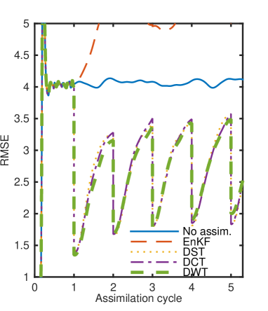
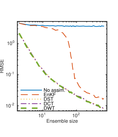
(a)	(b)

Fig. 1: Mean RMSE from 10 realizations for Lorenz 96 problem, the whole state observed, state dimension 256 (a) increasing analysis cycles with ensemble size 4, (b) increasing ensemble size, analysis cycle 1.

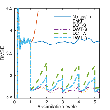
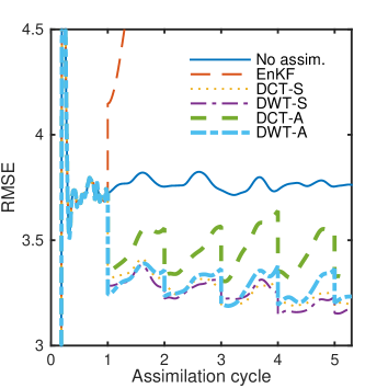
(a)	(b)

Fig. 2: Mean RMSE from 10 realizations for the Lorenz 96 problem, ensemble size 16, state dimension 256. (a) first 128 points observed, (b) first 64 points observed.

In the Lorenz 96 model (Lorenz, 2006), the state consists of one variable $\boldsymbol{X}_{t}\in\mathbb{R}^{K}$, $\boldsymbol{X}_{t}=\left(x_{1},\ldots,x_{K}\right)$, governed by the differential equations

$$\frac{dx_{j}}{dt}=x_{j-1}x_{j+1}-x_{j-1}x_{j-2}-x_{j}+F,\quad j=1,\ldots,K,$$

where the values of $x_{j-K}$ and $x_{j+K}$ are defined to be equal to $x_{j}$ for each $j=1,\ldots,K$, and $F$ is a parameter. We set the parameter $F=8$, which causes the system to be strongly chaotic. The timestep of model was set to $0.01\,\operatorname{s}$ and the analysis cycle was $1\,\operatorname{s}$. The data covariance was diagonal, with diagonal entries equal to $0.04$. The ensemble and the initial conditions for the truth were generated by sampling from $N(0.0005,0.01)$. The the ensemble and the truth were moved forward for 10 second, then the assimilation starts.

In the case when the whole state is observed, spectral filters with ensemble size $N=4$ (Fig. 1a) already decrease the error significantly compared to a run with no assimilation, while the standard EnKF actually increases the error. For all filters, the error eventually decreases with the ensemble size at the standard rate $N^{-1/2}$, but spectral EnKF shows the error decrease from the start, while the EnKF lags until the ensemble size is comparable to the state dimension, and even then its RMSE is significantly higher (Fig. 1b).

Next, consider the case when only the first $m$ points of a grid are observed. In the legend, DCT-S and DWT-S are the method with the discrete cosine transform, and the Coiflet 2,4 discrete wavelet transform, respectively, with the standard analysis update (8), while DCT-A and DWT-A use the augmented state method from Sect. 6.4. Figure  2 shows that the spectral diagonal method decrease the RMSE, while the standard EnKF is unstable. This observation is consistent with the result of Kelly et al. (2014), which shows that, for a class of dynamical systems, the EnKF remains within a bounded distance of truth if sufficiently large covariance inflation is used and if the whole state is observed. The augmented state method DWT-A with wavelet transformation gave almost the same analysis error as DCT-S, which is using the spectral diagonal filter with the exact observation matrix, while the cosine basis, which implies a homogenenous random field, resulted in a much larger error (method DCT-A). A similar behavior was seen with a smaller number of observed points as well, but the error reduction in spectral diagonal EnKF was smaller (not shown).

7.2 Shallow water equations

The shallow water equations can serve as a simplified model of atmospheric flow. The state $\boldsymbol{Y}=\left(\boldsymbol{h},\boldsymbol{u},\boldsymbol{v}\right)$ consists of water level height $\boldsymbol{h}$ and momentum $\boldsymbol{u},\boldsymbol{v}$ in $x$ and $y$ directions, governed by the differential equations of conservation of mass and momentum,

$$\frac{\partial\boldsymbol{h}}{\partial t}+\frac{\partial(\boldsymbol{uh})}{\partial x}+\frac{\partial(\boldsymbol{vh})}{\partial y} =0,$$

$$\frac{\partial(\boldsymbol{h}\boldsymbol{u})}{\partial t}+\frac{\partial}{\partial x}\left(\boldsymbol{h}\boldsymbol{u}^{2}+\frac{1}{2}g\boldsymbol{h}^{2}\right)+\frac{\partial(\boldsymbol{h}\boldsymbol{uv})}{\partial y} =0,$$

$$\frac{\partial(\boldsymbol{h}\boldsymbol{v})}{\partial t}+\frac{\partial(\boldsymbol{h}\boldsymbol{uv})}{\partial x}+\frac{\partial}{\partial y}\left(\boldsymbol{h}\boldsymbol{v}^{2}+\frac{1}{2}g\boldsymbol{h}^{2}\right) =0,$$

where $g$ is gravity acceleration, with reflective boundary conditions, and without Coriolis force or viscosity. The equations were discretized on a rectangular grid size $64\times 64$ with horizontal distance between grid points $150\,\operatorname{km}$ and advanced by the Lax-Wendroff method with the time step $1\,\operatorname{s}$. The initial values where water level $\boldsymbol{h}=10\,\operatorname{km}$, plus Gaussian water raise of height $1\,\operatorname{km}$, width $32$ nodes, in the center of the domain, and $\boldsymbol{u}=\boldsymbol{v}=0$. See Moler (2011, Chapter 18) for details.

We have used two independent initial conditions, one used for the truth and another for the ensemble and the free run. The only difference was the location of the initial wave. Both states were moved forward for 4 hours. Then the ensemble was created by adding random noise (with prescribed background covariance). Then, all states were moved forward for another hour, and assimilation starts $5\,\operatorname{h}$ after the model initialization. All assimilation methods start with the same forecast in the first assimilation cycle.

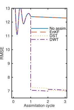
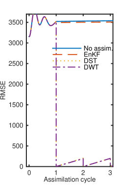
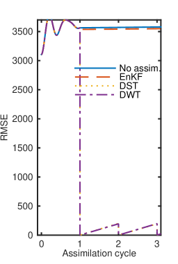
(a)	(b)	(c)

Fig. 3: RMSE of ensemble mean of one realization of three assimilation cycles (f - forecast error, a - analysis error). Full state was observed. The length of assimilation cycle 60 second, ensemble size 20. (a) water height (b) momentum in the $x$ direction (c) momentum in the $y$ direction

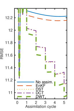
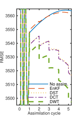
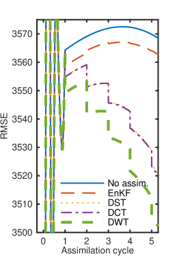
(a)	(b)	(c)

Fig. 4: Mean RMSE of ensemble mean from 5 independent repetitions. Ensemble size 20, only water height observed. (a) water height (b) momentum in the $x$ direction (c) momentum in the $y$ direction

The background covariance for initial ensemble perturbation was estimated using samples taken every second from time $t_{\text{start}}=4\,\operatorname{h}$ to time $t_{\mathrm{end}}=6\,\operatorname{h}$, and modified by tapering the sample covariance matrix $\mathbf{C}_{N}$ as $\mathbf{B}=\mathbf{C}_{N}\circ\mathbf{T},$ where the tapering matrix $\mathbf{T}$ had the block structure

$$\mathbf{T}=\left[\begin{matrix}\mathbf{A}&\mathbf{0}&\mathbf{0}\\ \mathbf{0}&\mathbf{A}&\mathbf{0}\\ \mathbf{0}&\mathbf{0}&\mathbf{A}\end{matrix}\right]+0.9\left[\begin{matrix}\mathbf{0}&\mathbf{A}&\mathbf{A}\\ \mathbf{A}&\mathbf{0}&\mathbf{A}\\ \mathbf{A}&\mathbf{A}&\mathbf{0}\end{matrix}\right],$$

where the entry between nodes $\left(i_{a},j_{a}\right)$ and $\left(i_{b},j_{b}\right)$ is $A_{a,b}=\exp(-|i_{a}-i_{b}|)\exp(-|j_{a}-j_{b}|)$. 2D tensor product FFT and DWT were used in the diagonal spectral EnKF. The observation error was taken with zero mean and variance $1000\,\operatorname{m^{2}}$ in $\boldsymbol{h}$ and $1000\,\operatorname{kg}\,\operatorname{m}\,\operatorname{s}^{-1}$ in $\boldsymbol{u}$ and $\boldsymbol{v}$. The forecast ensemble was created by adding random noise with the covariance $\mathbf{B}$ $4\,\operatorname{h}$ after the model initialization. To relax the ensemble members, the model was run for another hour before the assimilation started. So the first assimilation was performed 5 hours after the model initialization. After the first assimilation, another 4 assimilation cycles were performed every $60\,\operatorname{s}$.

When the full state is observed, the spectral diagonal method decreased the RMSE in all variables dramatically (Fig. 3), unlike the standard EnKF. When only the water level is observed, the RMSE in spectral diagonal EnKF decreases less, but still much more that in the standard EnKF (Fig. 4).

8 Conclusions

A version of the ensemble Kalman filter was presented, based on replacing the sample covariance by its diagonal in the spectral space, which provides a simple, efficient, and automatic localization. We have demonstrated efficient implementations for several classes of observation operators and data important in applications, including high-dimensional data defined on a continuous part of the domain, such as radar or satellize images. The spectral diagonal was proved rigorously to give a lower mean square error that the sample covariance. Computational experimens with the Lorenz 96 problem and the shallow water equations have shown that the method that the analysis error drops very fast for small ensembles, and the method is stable over multiple analysis cycles. The paper provides a new technology for data assimilation, which can work with minimal computational resources, because an implementation needs only an orthogonal transformation, such as the fast Fourier or discrete wavelet transform, and manipulation of vectors and diagonal matrices. Therefore, it should be of interest in applications.

Appendix A Properties of sample covariance matrix

Let $\boldsymbol{U}^{k}\sim N\left(\boldsymbol{0},\mathbf{C}\right)$ be independent random vectors in $\mathbb{R}^{n}$ or $\mathbb{C}^{n}$. For each $\boldsymbol{U}^{k}$, we have the Karhunen-Loève decomposition

$$\boldsymbol{U}^{k}=\sum_{j=1}^{n}\lambda_{j}^{1/2}\theta_{j,k}\boldsymbol{u}_{j},\quad\theta_{j,k}\sim N(0,1)\text{ independent.}$$ (15)

were $\lambda_{j}\geq 0$ are the eigenvalues and $\boldsymbol{u}_{j}$ orthonormal eigenvectors of the covariance matrix $\mathbf{C}$. Let $\mathbf{F}=\left[\boldsymbol{u}_{1},\ldots,\boldsymbol{u}_{n}\right]^{\ast}.$ By a direct computation, we have in the basis of the eigenvectors:

Lemma 2.

The random vector $\boldsymbol{U}_{\mathbf{F}}=\mathbf{FU}\sim N\left(\boldsymbol{0},\mathbf{C}_{\mathbf{F}}\right)$, where $\mathbf{C}_{\mathbf{F}}=\mathbf{FCF}^{\ast}$ is a diagonal matrix with $\lambda_{1},\ldots,\lambda_{n}$ on the diagonal.

Next, we use (15) to compute an expansion of the sample covariance entries.

Lemma 3.

Let $\mathbf{C}_{\mathbf{F}}^{N}$ be the sample covariance of $\boldsymbol{U}_{\mathbf{F}}^{1},\ldots,\boldsymbol{U}_{\mathbf{F}}^{N}$, cf., (5). Then,

$$(\mathbf{C}_{\mathbf{F}}^{N})_{i,j}=\frac{\left(\lambda_{i}\lambda_{j}\right)^{1/2}}{N-1}\left(\sum_{k=1}^{N}\theta_{i,k}\theta_{j,k}-\frac{1}{N}\sum_{l=1}^{N}\theta_{i,l}\sum_{m=1}^{N}\theta_{j,m}\right).$$ (16)

Proof. From the definition of the sample covariance,

$$\left(\mathbf{C}_{\mathbf{F}}^{N}\right)_{i.j} =\frac{1}{N-1}\sum_{k=1}^{N}\left(\boldsymbol{U}_{\mathbf{F}}^{k}-\bar{\boldsymbol{U}}_{\mathbf{F}}\right)_{i}\left(\boldsymbol{U}_{\mathbf{F}}^{k}-\bar{\boldsymbol{U}}_{\mathbf{F}}\right)_{j}^{\ast}$$

$$=\frac{1}{N-1}\sum_{k=1}^{N}\left(\boldsymbol{U}_{\mathbf{F}}^{k}-\frac{1}{N}\sum_{l=1}^{N}\boldsymbol{U}_{\mathbf{F}}^{l}\right)_{i}\left(\boldsymbol{U}_{\mathbf{F}}^{k}-\frac{1}{N}\sum_{m=1}^{N}\boldsymbol{U}_{\mathbf{F}}^{m}\right)_{j}^{\ast}$$

$$=\frac{1}{N-1}\left(\sum_{k=1}^{N}\left(\boldsymbol{U}_{\mathbf{F}}^{k}\right)_{i}\left(\boldsymbol{U}_{\mathbf{F}}^{k\ast}\right)_{j}-\frac{1}{N}\sum_{l=1}^{N}\left(\boldsymbol{U}_{\mathbf{F}}^{k}\right)_{l}\sum_{m=1}^{N}\left(\boldsymbol{U}_{\mathbf{F}}^{l}\right)_{m}\right)$$

$$=\frac{\left(\lambda_{i}\lambda_{j}\right)^{1/2}}{N-1}\left(\sum_{k=1}^{N}\theta_{i,k}\theta_{j,k}-\frac{1}{N}\sum_{l=1}^{N}\theta_{i,l}\sum_{m=1}^{N}\theta_{j,m}\right).\quad\rule{5.0pt}{5.0pt}$$

Finally, we use the expansion (16) to derive the variance of the sample covariance entries.

Lemma 4.

The variance of each entry of $\mathbf{C}_{\mathbf{F}}^{N}$ is

$$\operatorname{Var}[(\mathbf{C}_{\mathbf{F}}^{N})_{i,j}]=\left\{\begin{array}[c]{ll}\frac{2\lambda_{i}^{2}}{N-1}&\text{if }i=j,\\ \frac{\lambda_{i}\lambda_{j}}{N-1}&\text{if }i\neq j.\end{array}\right.$$

Proof. The sample covariance is unbiased estimate of the true covariance, so from Lemma 3,

$$\operatorname{Var}\left[(\mathbf{C}_{\mathbf{F}}^{N})_{i,i}\right] =\operatorname{E}\left[(\mathbf{C}_{\mathbf{F}}^{N})_{i,i}-\operatorname{E}\left[(\mathbf{C}_{\mathbf{F}}^{N})_{i,i}\right]\right]^{2}=\operatorname{E}\left[(\mathbf{C}_{\mathbf{F}}^{N})_{i,i}-(\mathbf{C}_{\mathbf{F}})_{i,i}\right]^{2}$$

$$=\operatorname{E}\left[\frac{\left(\lambda_{i}\lambda_{i}\right)^{1/2}}{N-1}\left(\sum_{k=1}^{N}\theta_{i,k}^{2}-\frac{1}{N}\sum_{k,l=1}^{N}\left(\theta_{i,k}\theta_{i,l}\right)\right)-\lambda_{i}\right]^{2}$$

$$=\frac{\lambda_{i}^{2}}{\left(N-1\right)^{2}}\operatorname{E}\left[\sum_{k=1}^{N}\theta_{i,k}^{2}\right]^{2}-\frac{2\lambda_{i}^{2}}{N\left(N-1\right)^{2}}\operatorname{E}\left[\sum_{k,l,m=1}^{N}\theta_{i,k}^{2}\theta_{i,l}\theta_{i,m}\right]$$

$$+\frac{\lambda_{i}^{2}}{N^{2}\left(N-1\right)^{2}}\operatorname{E}\left[\sum_{k,l=1}^{N}\theta_{i,k}\theta_{i,l}\right]^{2}-\frac{2\lambda_{i}^{2}}{\left(N-1\right)}\operatorname{E}\left[\sum_{k=1}^{N}\theta_{i,k}^{2}\right]$$

$$+\frac{2\lambda_{i}^{2}}{N\left(N-1\right)}\operatorname{E}\left[\sum_{k,l=1}^{N}\theta_{i,k}\theta_{i,l}\right]+\lambda_{i}^{2}.$$ (17)

The random variables $\theta_{i,k}$ are i.i.d., so it follows that

$$\operatorname{E}\left[\theta_{i,k}\theta_{i,l}\theta_{i,m}\theta_{i,n}\right]=\left\{\begin{array}[c]{ll}3&\quad\text{if }k=l=m=n,\\ 1&\quad\text{if }k=l,m=n,k\neq m,\\ 1&\quad\text{if }k=m,l=n,k\neq l,\\ 1&\quad\text{if }k=n,l=m,k\neq l,\\ 0&\quad\text{otherwise,}\end{array}\right.$$

and we can compute all the expected values in Eq. (17),

$$\operatorname{E}\left[\sum_{k=1}^{N}\theta_{i,k}^{2}\right]^{2} =\sum_{k=1}^{N}\operatorname{E}\left[\theta_{i,k}^{4}\right]+\sum_{k=1}^{N}\sum_{l=1,l\neq k}^{N}\operatorname{E}\left[\theta_{i,l}^{2}\theta_{i,k}^{2}\right]=3N+N(N-1)=N(N+2),$$

$$\operatorname{E}\left[\sum_{k,l,m=1}^{N}\theta_{i,k}^{2}\theta_{i,l}\theta_{i,m}\right] =\sum_{k=1}^{N}\operatorname{E}\left[\theta_{i,k}^{4}\right]+\sum_{k,l=1,l\neq k}^{N}\operatorname{E}\left[\theta_{i,k}^{2}\theta_{i,l}^{2}\right]=3N+N(N-1)=N(N+2),$$

$$\operatorname{E}\left[\sum_{k,l=1}^{N}\theta_{i,k}\theta_{i,l}\right]^{2} =\sum_{k,l,m,n=1}^{N}\operatorname{E}\left[\theta_{i,k}\theta_{i,l}\theta_{i,m}\theta_{i,n}\right]=\sum_{k=1}^{N}\operatorname{E}\left[\theta_{i,k}^{4}\right]+3\sum_{k,l=1,l\neq k}^{N}\operatorname{E}\left[\theta_{i,k}^{2}\theta_{i,l}^{2}\right]=3N^{2},$$

$$\operatorname{E}\left[\sum_{k=1}^{N}\theta_{i,k}^{2}\right] =\sum_{k=1}^{N}\operatorname{E}\left[\theta_{i,k}^{2}\right]=N,$$

$$\operatorname{E}\left[\sum_{k,l=1}^{N}\theta_{i,k}\theta_{i,l}\right] =\sum_{k=1}^{N}\operatorname{E}\left[\theta_{i,k}^{2}\right]=N.$$

Together, we get

$$\operatorname{Var}\left[(\mathbf{C}_{\mathbf{F}}^{N})_{i,i}\right]=\lambda_{i}^{2}\left(\frac{N(N+2)}{(N-1)^{2}}-\frac{2(N+2)}{(N-1)^{2}}+\frac{3}{(N-1)^{2}}-\frac{2N}{N-1}+\frac{2}{N-1}+1\right)=\frac{2\lambda_{i}^{2}}{N-1}.$$

The variance of the off-diagonal entry $(\mathbf{C}_{\mathbf{F}}^{N})_{i,j}$, $i\neq j$, is

$$\operatorname{Var}\left[(\mathbf{C}_{\mathbf{F}}^{N})_{i,j}\right] =\operatorname{E}\left[(\mathbf{C}_{\mathbf{F}}^{N})_{i,j}-\operatorname{E}\left[(\mathbf{C}_{\mathbf{F}}^{N})_{i,j}\right]\right]^{2}=\operatorname{E}\left[(\mathbf{C}_{\mathbf{F}}^{N})_{i,j}-(\mathbf{C}_{\mathbf{F}})_{i,j}\right]^{2}$$

$$=\operatorname{E}\left[\frac{\left(\lambda_{i}\lambda_{j}\right)^{1/2}}{N-1}\left(\sum_{k=1}^{N}\theta_{i,k}\theta_{j,k}-\frac{1}{N}\sum_{k,l=1}^{N}\left(\theta_{i,k}\theta_{j,l}\right)\right)-0\right]^{2}$$

$$=\frac{\lambda_{i}\lambda_{j}}{\left(N-1\right)^{2}}\operatorname{E}\left[\sum_{k=1}^{N}\theta_{i,k}\theta_{j,k}\right]^{2}-\frac{2\lambda_{i}\lambda_{j}}{N\left(N-1\right)^{2}}\operatorname{E}\left[\sum_{k,l,m=1}^{N}\theta_{i,k}\theta_{j,k}\theta_{i,l}\theta_{j,m}\right]$$

$$+\frac{\lambda_{i}\lambda_{j}}{N^{2}\left(N-1\right)^{2}}\operatorname{E}\left[\sum_{k,l=1}^{N}\theta_{i,k}\theta_{j,l}\right]^{2}.$$ (18)

The integrals in Eq. (18) are

$$\operatorname{E}\left[\sum_{k=1}^{N}\theta_{i,k}\theta_{j,k}\right]^{2} =\sum_{k,l=1}^{N}\operatorname{E}\left[\theta_{i,k}\theta_{j,k}\theta_{i,l}\theta_{j,l}\right]=\sum_{k,l=1}^{N}\operatorname{E}\left[\theta_{i,k}\theta_{i,l}\right]\operatorname{E}\left[\theta_{j,k}\theta_{j,l}\right]$$

$$=\sum_{k=1}^{N}\operatorname{E}\left[\theta_{i,k}\theta_{i,k}\right]\operatorname{E}\left[\theta_{j,k}\theta_{j,l}\right]=N,$$

$$\operatorname{E}\left[\sum_{k,l,m=1}^{N}\theta_{i,k}\theta_{j,k}\theta_{i,l}\theta_{j,m}\right] =\sum_{k,l,m=1}^{N}\operatorname{E}\left[\theta_{i,k}\theta_{i,l}\right]\operatorname{E}\left[\theta_{j,k}\theta_{j,m}\right]=\sum_{k=1}^{N}\operatorname{E}\left[\theta_{i,k}\theta_{i,k}\right]\operatorname{E}\left[\theta_{j,k}\theta_{j,k}\right]=N,$$

$$\operatorname{E}\left[\sum_{k,l=1}^{N}\theta_{i,k}\theta_{j,l}\right]^{2} =\operatorname{E}\left[\sum_{k=1}^{N}\theta_{i,k}\sum_{k,l=1}^{N}\theta_{j,l}\right]^{2}=\operatorname{E}\left[\sum_{k=1}^{N}\theta_{i,k}\right]^{2}\operatorname{E}\left[\sum_{l=1}^{N}\theta_{j,l}\right]^{2}=N^{2}.$$

So, the variance of an off-diagonal element is $\operatorname{Var}\left[(\mathbf{C}_{\mathbf{F}}^{N})_{i,j}\right]=\frac{\lambda_{i}\lambda_{j}}{(N-1)^{2}}\left(N-2+1\right)=\frac{\lambda_{i}\lambda_{j}}{N-1}$.

References

• Anderson and Moore (1979) Anderson, B. D. O. and Moore, J. B.: Optimal filtering, Prentice-Hall, Englewood Cliffs, N.J., 1979.
• Anderson (2001) Anderson, J. L.: An Ensemble Adjustment Kalman Filter for Data Assimilation, Monthly Weather Review, 129, 2884–2903, 10.1175/1520-0493(2001)129$<$2884:AEAKFF$>$2.0.CO;2, 2001.
• Beezley et al. (2011) Beezley, J. D., Mandel, J., and Cobb, L.: Wavelet Ensemble Kalman Filters, in: Proceedings of IEEE IDAACS’2011, Prague, September 2011, vol. 2, pp. 514–518, IEEE, 10.1109/IDAACS.2011.6072819, 2011.
• Berre (2000) Berre, L.: Estimation of synoptic and mesoscale forecast error covariances in a limited-area model, Monthly Weather Review, 128, 644–667, 10.1175/1520-0493(2000)128$<$0644:EOSAMF$>$2.0.CO;2, 2000.
• Boer (1983) Boer, G. J.: Homogeneous and Isotropic Turbulence on the Sphere, Journal of the Atmospheric Sciences, 40, 154–163, 10.1175/1520-0469(1983)040$<$0154:HAITOT$>$2.0.CO;2, 1983.
• Buehner and Charron (2007) Buehner, M. and Charron, M.: Spectral and spatial localization of background-error correlations for data assimilation, Quarterly Journal of the Royal Meteorological Society, 133, 615–630, 10.1002/qj.50, 2007.
• Burgers et al. (1998) Burgers, G., van Leeuwen, P. J., and Evensen, G.: Analysis Scheme in the Ensemble Kalman Filter, Monthly Weather Review, 126, 1719–1724, 1998.
• Courtier et al. (1998) Courtier, P., Andersson, E., Heckley, W., Vasiljevic, D., Hamrud, M., Hollingsworth, A., Rabier, F., Fisher, M., and Pailleux, J.: The ECMWF implementation of three-dimensional variational assimilation (3D-Var). I: Formulation, Quarterly Journal of the Royal Meteorological Society, 124, 1783–1807, 10.1002/qj.49712455002, 1998.
• Da Prato (2006) Da Prato, G.: An introduction to infinite-dimensional analysis, Springer-Verlag, Berlin, 10.1007/3-540-29021-4, 2006.
• Daubechies (1992) Daubechies, I.: Ten lectures on wavelets, vol. 61 of CBMS-NSF Regional Conference Series in Applied Mathematics, Society for Industrial and Applied Mathematics (SIAM), Philadelphia, PA, 10.1137/1.9781611970104, 1992.
• Evensen (2009) Evensen, G.: Data Assimilation: The Ensemble Kalman Filter, Springer, 2nd edn., 10.1007/978-3-642-03711-5, 2009.
• Furrer and Bengtsson (2007) Furrer, R. and Bengtsson, T.: Estimation of high-dimensional prior and posterior covariance matrices in Kalman filter variants, J. Multivariate Anal., 98, 227–255, 10.1016/j.jmva.2006.08.003, 2007.
• Gaspari and Cohn (1999) Gaspari, G. and Cohn, S. E.: Construction of correlation functions in two and three dimensions, Quarterly Journal of the Royal Meteorological Society, 125, 723–757, 10.1002/qj.49712555417, 1999.
• Hunt et al. (2007) Hunt, B. R., Kostelich, E. J., and Szunyogh, I.: Efficient data assimilation for spatiotemporal chaos: a local ensemble transform Kalman filter, Physica D: Nonlinear Phenomena, 230, 112–126, 10.1016/j.physd.2006.11.008, 2007.
• Kalman (1960) Kalman, R. E.: A New Approach to Linear Filtering and Prediction Problems, Transactions of the ASME – Journal of Basic Engineering, Series D, 82, 35–45, 1960.
• Kalnay (2003) Kalnay, E.: Atmospheric Modeling, Data Assimilation and Predictability, Cambridge University Press, 2003.
• Kelly et al. (2014) Kelly, D. T. B., Law, K. J. H., and Stuart, A. M.: Well-Posedness and Accuracy of the Ensemble Kalman Filter in Discrete and Continuous Time, Nonlinearity, 27, 2579–2603, 10.1088/0951-7715/27/10/2579, 2014.
• Kwiatkowski and Mandel (2014) Kwiatkowski, E. and Mandel, J.: Convergence of the Square Root Ensemble Kalman Filter in the Large Ensemble Limit, SIAM/ASA Journal on Uncertainty Quantification, p. In print, arXiv:1404.4093, 2014.
• Lahoz et al. (2010) Lahoz, W., Khattatov, B., and Menard, R., eds.: Data Assimilation: Making Sense of Observations, Springer, 10.1007/978-3-540-74703-1, 2010.
• Le Gland et al. (2011) Le Gland, F., Monbet, V., and Tran, V.-D.: Large sample asymptotics for the ensemble Kalman filter, in: The Oxford Handbook of Nonlinear Filtering, edited by Crisan, D. and Rozovskiǐ, B., pp. 598–631, Oxford University Press, 2011.
• Lorenz (2006) Lorenz, E. N.: Predictability - a problem partly solved, in: Predictability of Weather and Climate, edited by Palmer, T. and Hagendorn, R., pp. 40–58, Cambridge University Press, 2006.
• Mandel et al. (2010a) Mandel, J., Beezley, J., Cobb, L., and Krishnamurthy, A.: Data driven computing by the morphing fast Fourier transform ensemble Kalman filter in epidemic spread simulations, Procedia Computer Science, 1, 1215–1223, 10.1016/j.procs.2010.04.136, 2010a.
• Mandel et al. (2010b) Mandel, J., Beezley, J. D., and Kondratenko, V. Y.: Fast Fourier Transform Ensemble Kalman Filter with Application to a Coupled Atmosphere-Wildland Fire Model, in: Computational Intelligence in Business and Economics, Proceedings of MS’10, edited by Gil-Lafuente, A. M. and Merigo, J. M., pp. 777–784, World Scientific, 10.1142/9789814324441_0089, 2010b.
• Mandel et al. (2011) Mandel, J., Cobb, L., and Beezley, J. D.: On the convergence of the ensemble Kalman filter, Applications of Mathematics, 56, 533–541, 10.1007/s10492-011-0031-2, 2011.
• Moler (2011) Moler, C.: Experiments with MATLAB, http://www.mathworks.com/moler/exm, accessed December 2014, 2011.
• Pannekoucke et al. (2007) Pannekoucke, O., Berre, L., and Desroziers, G.: Filtering Properties of Wavelets For Local Background-Error Correlations, Quarterly Journal of the Royal Meteorological Society, 133, 363–379, 10.1002/qj.33, 2007.
• Parrish and Derber (1992) Parrish, D. F. and Derber, J. C.: The National Meteorological Center’s Spectral Statistical-Interpolation Analysis System, Monthly Weather Review, 120, 1747–1763, 10.1175/1520-0493(1992)120$<$1747:TNMCSS$>$2.0.CO;2, 1992.
• Sakov and Bertino (2010) Sakov, P. and Bertino, L.: Relation Between Two Common Localisation Methods for the EnKF, Computational Geosciences, in print, 10.1007/s10596-010-9202-6, 2010.