The parallel replica method for computing equilibrium averages of Markov chains

Abstract.

An algorithm is proposed for computing equilibrium averages of Markov chains which suffer from metastability – the tendency to remain in one or more subsets of state space for long time intervals. The algorithm, called the parallel replica method (or ParRep), uses many parallel processors to explore these subsets more efficiently. Numerical simulations on a simple model demonstrate consistency of the method. A proof of consistency is given in an idealized setting. The parallel replica method can be considered a generalization of A.F. Voter’s parallel replica dynamics, originally developed to efficiently simulate metastable Langevin stochastic dynamics.

1. Introduction

This article concerns the problem of computing equilibrium averages of time homogeneous, ergodic Markov chains in the presence of metastability. A Markov chain is said to be metastable if it has typically very long sojourn times in certain subsets of state space, called metastable sets. A new method, called the parallel replica method (or ParRep), is proposed for efficiently simulating equilibrium averages in this setting.

Markov chains are widely used to model physical systems. In computational statistical physics – the main setting for this article – Markov chains are used to understand macroscopic properties of matter, starting from a mesoscopic or microscopic description. Equilibrium averages then correspond to bulk properties of the physical system under consideration, like average density or internal energy. A popular class of such models are the Markov State Models [4, 9, 11]. Markov chains also arise as time discretizations of continuous time models like the Langevin dynamics [8], a popular stochastic model for molecular dynamics. For examples of Markov chain models not obtained from an underlying continuous time dynamics, see for example [3, 12]. It should be emphasized that the discrete in time setting is generic – even if the underlying model is continuous in time, what must be simulated in practice is a time-discretized version.

In computational statistical physics, metastability arises from entropic barriers, which are bottlenecks in state space, as well as energetic barriers, which are regions separating metastable states through which crossings are unlikely (due to, for example, high energy saddle points in a potential energy landscape separating the states). See Figures 1–2 for simple examples of entropic and energetic barriers.

The method proposed here is closely related to a recently proposed algorithm [1], also called ParRep, for efficient simulation of metastable Markov chains on a coarsened state space. That algorithm can be considered an adaptation of A.F. Voter’s parallel replica dynamics [14] to a discrete time setting. (For a mathematical analysis of A.F. Voter’s original algorithm, see [7].) ParRep was shown to be consistent with an analysis based on quasistationary distributions (QSDs), or local equilibria associated with each metastable set. ParRep uses parallel processing to explore phase space more efficiently in real time. A cost of the parallelization is that only a coarse version of the Markov chain dynamics, defined on the original state space modulo the collection of metastable sets, is obtained. In this article it is shown that a simple modification of the ParRep algorithm of [1] nonetheless allows for computation of equilibrium averages of the original, uncoarsened Markov chain.

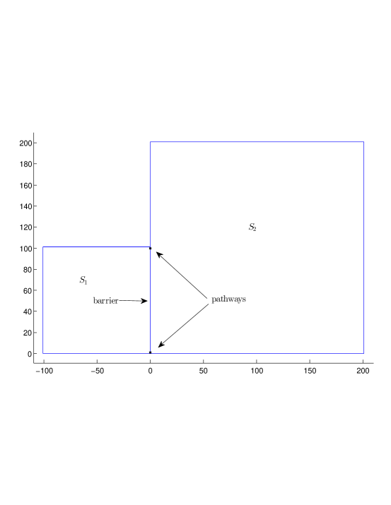
Figure 1. A random walk $X_{n}$ on state space $\{-1,-2,\ldots,-100\}^{2}\cup\{1,2,\ldots,200\}^{2}$ with an entropic barrier. At each step, a direction up, down, left or right is selected at random, each with probability $1/4$. Then $X_{n}$ moves one unit in this direction, provided this does not result in crossing a barrier, i.e., one of the edges of the two boxes pictured. The walk can cross from the left box to the right box only through the narrow pathways indicated. The metastable sets are ${\mathcal{S}}=\{S_{1},S_{2}\}$.

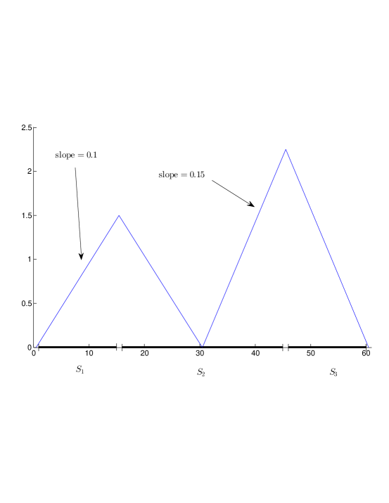
Figure 2. A random walk $X_{n}$ on state space $\{1,2,\ldots,60\}$ with energy barriers. The random walk moves one unit left or right according to a biased coin flip: If $X_{n}=x$ and the slope of the pictured graph at $x$ is $m$, then with probability $1/2+m$, $X_{n+1}=\max\{x-1,1\}$, and with probability $1/2-m$, $X_{n+1}=\min\{x+1,60\}$. The metastable sets are ${\mathcal{S}}=\{S_{1},S_{2},S_{3}\}$.

The ParRep algorithm proposed here is very general. It can be applied to any Markov chain, and gains in efficiency can be expected when the chain is metastable and the metastable sets can be properly identified (either a priori or on the fly). In particular, it can be applied to metastable Markov chains with both energetic and entropic barriers, and no assumptions about barrier heights, temperature or reversibility are required. While there exist many methods for sampling from a distribution, most methods, particularly in Markov chain Monte Carlo [10], rely on a priori knowledge of relative probabilities of the distribution. In contrast with these methods, ParRep does not require any information about the equilibrium distribution of the Markov chain.

The article is organized as follows. Section 2 defines the QSD and notation used throughout. Section 3 introduces the ParRep algorithm for computing equilibrium averages (Algorithm 2). In Section 4, consistency of the algorithm is demonstrated on the simple models pictured in Figures 1 and 2. A proof of consistency in an idealized setting is given in the Appendix. Some concluding remarks are made in Section 5.

2. Notation and the quasistationary distribution

Throughout, $(X_{n})_{n\geq 0}$ is a time homogeneous Markov chain on a standard Borel state space, and ${\mathbb{P}}_{\xi}$ is the associated measure when $X_{0}\sim\xi$, where $\sim$ denotes equality in law. All sets and functions are assumed measurable without explicit mention. The collection of metastable sets will be written ${\mathcal{S}}$, with elements of ${\mathcal{S}}$ denoted by $S$. Formally, ${\mathcal{S}}$ is simply a set of disjoint subsets of state space.

Definition 1.

A probability measure $\nu$ with support in $S$ is called a quasistationary distribution (QSD) if for all $n\geq 0$ and all $A\subset S$,

$$\nu(A)={\mathbb{P}}_{\nu}\left(X_{n}\in A\,|\,X_{1}\in S,\ldots,X_{n}\in S\right).$$

That is, if $X_{n}\sim\nu$, then conditionally on $X_{n+1}\in S$, $X_{n+1}\sim\nu$. It is not hard to check that, if for every probability measure $\xi$ supported in $S$ and every $A\subset S$,

$$\nu(A)=\lim_{n\to\infty}{\mathbb{P}}_{\xi}\left(X_{n}\in A\,|\,X_{1}\in S,\ldots,X_{n}\in S\right),$$ (2.1)

then $\nu$ is the unique QSD in $S$. Informally, if (2.1) holds, then $(X_{n})_{n\geq 0}$ is close to $\nu$ whenever it spends a sufficiently long time in $S$ without leaving. Of course $\nu$ depends on $S$, but this will not be indicated explicitly.

3. The ParRep algorithm

Let $(X_{n})_{n\geq 0}$ be ergodic with equilibrium measure $\mu$, and fix a bounded real-valued function $f$ defined on state space. The output of ParRep is an estimate of the average of $f$ with respect to $\mu$. The algorithm requires existence of a unique QSD in each metastable set, so it is assumed for each $S\in{\mathcal{S}}$ there is a unique $\nu$ satisfying (2.1). This assumption holds under very general mixing conditions; see [1].

The user-chosen parameters of the algorithm are the number of replicas, $N$; the decorrelation and dephasing times, $T_{corr}$ and $T_{phase}$; and a polling time, $T_{poll}$. The parameters $T_{corr}$ and $T_{phase}$ are closely related to the time needed to reach the QSD; both may depend on $S\in{\mathcal{S}}$. To emphasize this, sometimes $T_{corr}(S)$ or $T_{phase}(S)$ are written. The parameter $T_{poll}$ is a polling time at which the parallel replicas resynchronize. See below for further discussion.

Algorithm 2.

Set the simulation clock to zero: $T_{sim}=0$, and set $f_{sim}=0$. Then iterate the following:

• Decorrelation Step.

  Evolve $(X_{n})_{n\geq 0}$ from time $n=T_{sim}$ until time $n=\sigma$, where $\sigma$ is the smallest number $n\geq T_{sim}+T_{corr}-1$ such that there exists $S\in{\mathcal{S}}$ with $X_{n}\in S,\,X_{n-1}\in S,\ldots,X_{n-T_{corr}+1}\in S$. Meanwhile, update

  $$f_{sim}=f_{sim}+\sum_{n=T_{sim}+1}^{\sigma}f(X_{n}).$$

  Then set $T_{sim}=\sigma$ and proceed to the Dephasing Step, with $S$ now the metastable state having $X_{\sigma}\in S$.

• Dephasing Step.

  Generate $N$ independent samples, $x_{1},\ldots,x_{N}$, of the QSD $\nu$ in $S$. Then proceed to the Parallel Step.

• Parallel Step.

  (i) Set $M=1$ and $\tau_{acc}=0$. Let $(X_{n}^{1})_{n\geq 0},\ldots,(X_{n}^{N})_{n\geq 0}$ be replicas of $(X_{n})_{n\geq 0}$, that is, Markov chains with the same law as $(X_{n})_{n\geq 0}$ which are independent of $(X_{n})_{n\geq 0}$ and one another. Set $X_{0}^{1}=x_{1}$,…, $X_{0}^{N}=x_{N}$.

  (ii) Evolve all the replicas from time $n=(M-1)T_{poll}$ to time $n=MT_{poll}$.

  (iii) If none of the replicas leave $S$ during this time, update

  $$f_{sim}=f_{sim}+\sum_{i=1}^{N}\sum_{j=(M-1)T_{poll}+1}^{MT_{poll}}f(X_{j}^{i}),$$ (3.1)

  $$\tau_{acc}=\tau_{acc}+NT_{poll},$$

  $$M=M+1,$$

  and return to (ii) above. Otherwise, let $K$ be the smallest number such that $(X_{n}^{K})_{n\geq 0}$ leaves $S$ during this time, let $\tau^{K}\in[(M-1)T_{poll}+1,MT_{poll}]$ be the corresponding first exit time, and update

  $$f_{sim}=f_{sim}+\sum_{i=1}^{K-1}\sum_{j=(M-1)T_{poll}+1}^{MT_{poll}}f(X_{j}^{i})+\sum_{j=(M-1)T_{poll}+1}^{\tau^{K}}f(X_{j}^{K}),$$ (3.2)

  $$\tau_{acc}=\tau_{acc}+(K-1)T_{poll}+(\tau^{K}-(M-1)T_{poll}).$$

  Then update $T_{sim}=T_{sim}+\tau_{acc}$, set $X_{T_{sim}}=X_{acc}:=X_{\tau^{K}}^{K}$, and return to the Decorrelation Step.

See Figure 3 for an illustration of the Parallel Step. The key quantity in the algorithm is the running average $f_{sim}/T_{sim}$, which is an estimate of the average of $f$ with respect to the equilibrium measure $\mu$:

$$\frac{f_{sim}}{T_{sim}}\approx\int f\,d\mu.$$

Some remarks on Algorithm 2 are in order.

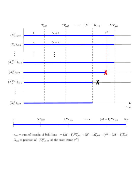
Figure 3. Visualization of the Parallel Step of Algorithm 2. The crosses represent exits from $S$. After $M$ loops internal to the Parallel Step, two of the replicas leave $S$, with $(X_{n}^{K})_{n\geq 0}$, the one among these having the smallest index $K$, leaving at time $\tau^{K}$. The trajectories of all the replicas can be concatenated into a single long trajectory of length $\tau_{acc}$. This single long trajectory is obtained by running through the columns of width $T_{poll}$ from top to bottom, starting at the far left, in the order $1,2,\ldots,N+1,N+2,\ldots$ indicated. The time marginals of this long trajectory (except its right endpoint) are all distributed according to the QSD in $S$.

• The Decorrelation Step. The purpose of the Decorrelation Step is to reach the QSD in some metastable set. Indeed, the Decorrelation Step terminates exactly when $(X_{n})_{n\geq 0}$ has spent $T_{corr}$ consecutive time steps in some metastable set $S$ – so the position of $(X_{n})_{n\geq 0}$ at the end of the Decorrelation Step can be considered an approximate sample from $\nu$, the QSD in $S$. The error in this approximation is controlled by the parameter $T_{corr}$. Larger values of $T_{corr}$ lead to increased accuracy but lessened efficiency; see the numerical tests in Section 4 below, in particular Figures 4 and 6. During the Decorrelation Step, the dynamics of $(X_{n})_{n\geq 0}$ is exact, so the contribution to $f_{sim}$ from the Decorrelation Step is exact.

• The Dephasing Step. The Dephasing Step requires sampling $N$ iid copies of the QSD in $S$, where $S$ is the metastable set from the end of the Decorrelation Step. The practitioner has flexibility in sampling these points. Essentially, one has to sample $N$ endpoints of trajectories of $(X_{n})_{n\geq 0}$ that have remained in $S$ for a long enough time, with this time being controlled by the parameter $T_{phase}$. For example, the Dephasing Step can be done with rejection sampling, keeping trajectories which have remained in $S$ for time $T_{phase}$. Alternatively, the QSD samples may be obtained via techniques related to the Fleming-Viot process; for details see [1] and [2]. This technique can be summarized as follows: $N$ replicas of $(X_{n})_{n\geq 0}$, all starting in $S$, are independently evolved until one or several leave $S$; then each replica which left $S$ is restarted from the current position of another replica still inside $S$, chosen uniformly at random. After time $T_{phase}$ this procedure stops and the current positions of the replicas are used as the $N$ required samples of $\nu$.

  Under mild mixing conditions, convergence to the QSD is very fast. More precisely, the limit in the right hand side of (2.1) converges to $\nu$ geometrically fast in total variation norm [1]. An analysis of the error associated with not exactly reaching the QSD will be the focus of another work. For an analysis of the error associated with not reaching the QSD in the original continuous-in-time version of the algorithm, see [13]. In the metastable setting considered here, the average time to (approximately) reach the QSD in $S$ is assumed much smaller than the average time, starting at the QSD, to leave $S$. Indeed, this assumption can be considered the very definition of metastability. Gains in efficiency in ParRep are limited by the degree of metastability; see [2] and the discussion in Section 4 below.

  It is emphasized that $f_{sim}$ and $T_{sim}$ are left unchanged during the Dephasing Step. Contributions to $f_{sim}$ and $T_{sim}$ come only from the Decorrelation and Parallel Steps.

• The Parallel Step. The purpose of the Parallel Step is twofold. First, it simulates an exit event from $S$, the metastable set from the end of the Decorrelation Step, starting from the QSD in $S$. This is consistent with the exit event that would have been observed if, in the Decorrelation Step, $(X_{n})_{n\geq 0}$ had been allowed to continue evolving until leaving $S$:

  Theorem 3.

  (Proposition 4.5 of [1].) Suppose the QSD sampling in the Dephasing Step of Algorithm 2 is exact. Then in the Parallel Step, $(\tau_{acc},X_{acc})\sim(\tau,X_{\tau})$, where $X_{0}\sim\nu$, with $\nu$ the QSD in $S$ and $\tau:=\min\{n\geq 0\,:\,X_{n}\notin S\}$.

  The gain in efficiency in ParRep, compared to direct serial simulation, comes from the use of parallel processing in the Parallel Step. The wall-clock time speedup – the ratio of average serial simulation time to the ParRep simulation time of the exit event – scales like $N$, though the gain in efficiency in ParRep as a whole depends also on $T_{corr}$, $T_{phase}$ and the degree of metastability of the sets in ${\mathcal{S}}$.

  Second, the Parallel Step includes a contribution to $f_{sim}$. As the fine scale dynamics of $(X_{n})_{n\geq 0}$ in $S$ are not retained in the Parallel step, this contribution is not exact. It is, however, consistent on average, which is sufficient for the computation of equilibrium averages. This can be understood as follows. Concatenate all the trajectories of all the replicas into a single long trajectory by following the procedure indicated in Figure 3. The resulting trajectory has a probability law that is of course different from that of $(X_{n})_{n\geq 0}$ starting from the QSD $\nu$ in $S$. However, in light of Definition 1, the time marginals of this trajectory (except the right endpoint) are all distributed according to $\nu$. Moreover, from Theorem 3, the total length of this concatenated trajectory has the same law as that of $(X_{n})_{n\geq 0}$ started from the QSD in $S$ and stopped at the first exit time from $S$. So by linearity of expectation, the contribution to $f_{sim}$ from the Parallel Step is consistent on average. See the Appendix for proofs of these statements in an idealized setting.

• Other remarks. The parameter $T_{poll}$ is a polling time at which the possibly asynchronous parallel processors in the Parallel Step resynchronize. For the Parallel Step to be finished correctly, one has to wait until the first $K$ processors have completed $MT_{poll}$ time steps. If the processors are nearly synchronous or communication between them is cheap, one can take $T_{poll}=1$.

  The metastable sets ${\mathcal{S}}$ need not be known a priori. In many applications, they can be identified on the fly; for example, when the metastable sets are the basins of attraction of a potential energy, they can be found efficiently on the fly by gradient descent. The reader is referred to [2] as well as [1] and references therein for examples of successful applications of related versions of ParRep in this setting.

4. Numerical tests

4.1. Example 1: Entropic barrier

Consider the Markov chain from Figure 1 on state space $\{-1,-2,\ldots,-100\}^{2}\cup\{1,2,\ldots,200\}^{2}$. The Markov chain evolves according to a random walk: at each time step it moves one unit up, down, left or right each with probability $1/4$, provided the result is inside state space; if not, the move is rejected and the position stays the same. There is one exception: If the current position is $(-1,1)$ or $(-1,100)$ and a move to the right is proposed, then the next position is $(1,1)$ or $(1,100)$, respectively; and if the current position is $(1,1)$ or $(1,100)$ and a move to the left is proposed, then the next position is $(-1,1)$ or $(-1,100)$, respectively. This Markov chain is ergodic with respect to the uniform distribution $\mu_{unif}$ on state space.

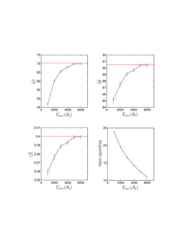
Figure 4. Equilibrium average values and (average) time speedup vs. $T_{corr}(S_{1})$ in ParRep simulations of the Markov chain from Example 1, with $N=100$. The straight lines correspond to exact values. ParRep simulations were stopped when $T_{sim}$ first exceeded $5\times 10^{9}$, and error bars are standard deviations obtained from $100$ independent trials.

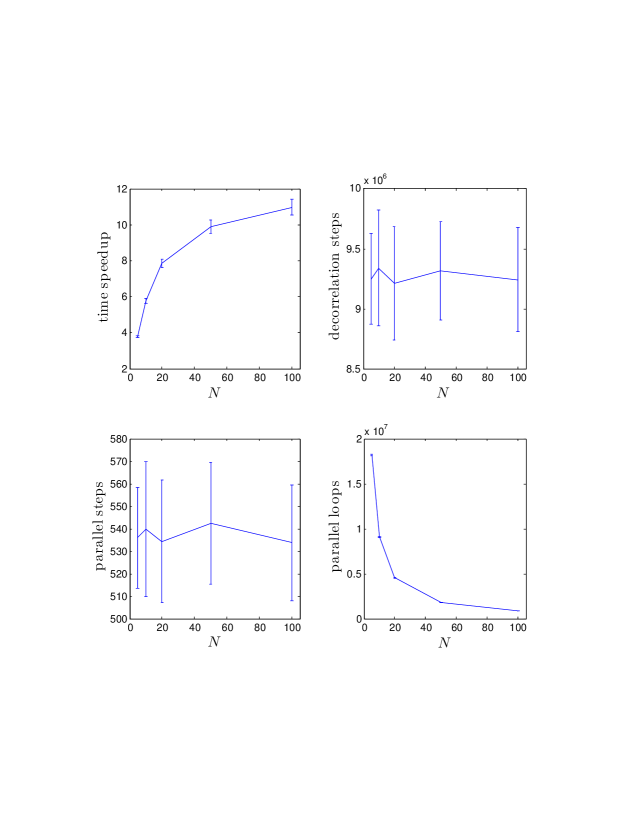
Figure 5. Average time speedup factor, number of decorrelation steps, number of parallel steps, and number of parallel loops in ParRep simulations of the Markov chain from Example 1, with $T_{corr}(S_{1})=6000$. ParRep simulations were stopped when $T_{sim}$ first exceeded $10^{8}$, and error bars are standard deviations obtained from $100$ independent trials.

ParRep was performed on this system with $S_{1}:=\{-1,-2,\ldots,-100\}^{2}$, $S_{2}:=\{1,2,\ldots,200\}^{2}$, and ${\mathcal{S}}=\{S_{1},S_{2}\}$. Parameters were always chosen so that $T_{corr}=T_{phase}$ and $T_{corr}(S_{2})=4T_{corr}(S_{1})$, and QSD samples from the Dephasing Step were obtained using the Fleming-Viot-based technique described above.

With $N=100$ replicas and various values of $T_{corr}(S_{1})$, ParRep was used to obtain average $x$- and $y$-coordinates with respect to $\mu_{unif}$ as well as the $\mu_{unif}$-probability to be in the upper half of the right hand side box, denoted by:

$$\langle x\rangle:=\int x\,d\mu_{unif},\qquad\langle y\rangle:=\int y\,d\mu_{unif},$$

$$\langle f\rangle:=\int 1_{y\in[101,200]}\,d\mu_{unif}.$$

Here $1_{A}$ denotes the indicator function of $A$. See Figure 4. Also computed was the average time speedup: namely, $T_{sim}$ divided by the “wall clock time,” defined as follows. Like $T_{sim}$, the wall clock time stars at zero. It increases by $1$ during each time step of $(X_{n})_{n\geq 0}$ in the Decorrelation Step (consistent with $T_{sim}$), while it increases by $MT_{poll}$ in the Parallel Step (unlike $T_{sim}$, which increases by $\tau_{acc}$). The wall clock time also increases by $T_{phase}$ during the dephasing step (where $T_{sim}$ does not increase at all). Informally, the wall clock time corresponds to true clock time in an idealized setting where all the processors always compute one time step of $(X_{n})_{n\geq 0}$ in exactly $1$ unit of time, and communication between processors takes zero time. As $T_{corr}$ increases, the time speedup decreases, but accuracy increases.

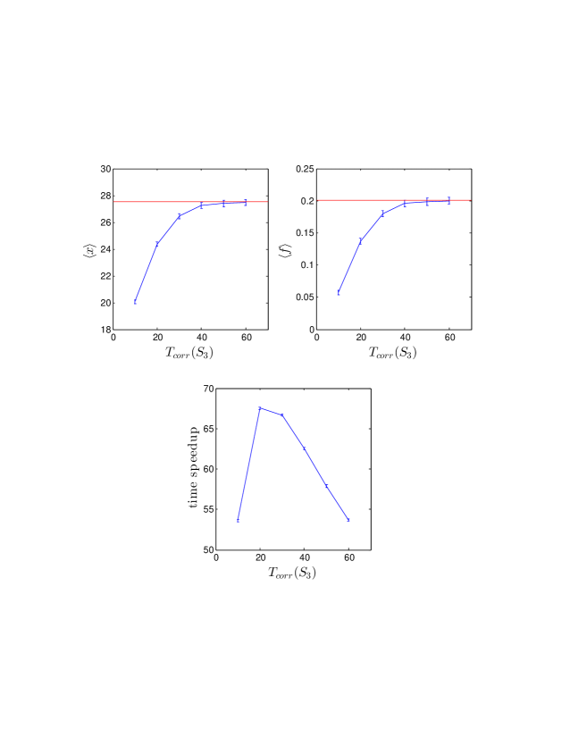
Figure 6. Equilibrium average values and (average) time speedup vs. $T_{corr}(S_{3})$ in ParRep simulations of the Markov chain from Example 2, with $N=100$. The straight lines correspond to exact values. ParRep simulations were stopped when $T_{sim}$ first exceeded $10^{9}$, and error bars are standard deviations obtained from $100$ independent trials. For the smallest value of $T_{corr}(S_{3})$, the Markov chain is typically close to the edges of $S_{1}$, $S_{2}$ or $S_{3}$, which results in shorter parallel steps and thus a smaller time speedup.

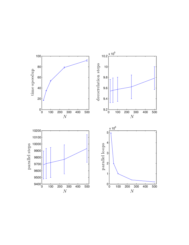
Figure 7. Average time speedup factor, number of decorrelation steps, number of parallel steps, and number of parallel loops in ParRep simulations of the Markov chain from Example 2, when $T_{corr}(S_{3})=60$. ParRep simulations were stopped when $T_{sim}$ first exceeded $10^{8}$, and error bars are standard deviations obtained from $100$ independent trials.

Figure 5 shows the dependence of time speedup on the number of replicas, $N$, when $T_{corr}(S_{1})=6000$. To illuminate the dependence of time speedup on $N$, Figure 5 also includes the average (total) number of decorrelation steps, parallel steps, and parallel loops (i.e., loops internal to the parallel step – in the notation of Algorithm 2, there are $M$ loops internal to the parallel step). As $N$ increases, the number of parallel loops decreases sharply, while the number of parallel steps and decorrelation steps remain nearly constant. Thus, with increasing $N$ the wall clock time spent in the parallel step falls quickly. The time speedup, however, is limited by the wall clock time spent in the decorrelation step, and so it levels off with increasing $N$. The value of $N$ at which this leveling off occurs depends on the degree of metastability in the problem, or slightly more precisely, the ratios, over all $S\in{\mathcal{S}}$, of the time scale for leaving $S$ to the time scale for reaching the QSD in $S$. In the limit as this ratio approaches infinity, the time speedup grows like $N$. See [2] for a discussion of this issue in a continuous time version of ParRep.

4.2. Example 2: Energetic barrier

Consider the Markov chain from Figure 2 on state space $\{1,\ldots,60\}$. The Markov chain evolves according to a biased random walk: If $X_{n}=x$, then with probability $p_{x}$, $X_{n+1}=\max\{1,x-1\}$, while with probability $1-p_{x}$, $X_{n+1}=\min\{60,x+1\}$. Here,

$$p_{x}:=\begin{cases}0.6,&x\in\{1,\ldots,15\}\\ 0.4,&x\in\{16,\ldots,30\}\\ 0.65,&x\in\{31,\ldots,45\}\\ 0.35,&x\in\{46,\ldots,60\}.\end{cases}$$

The equilibrium distribution $\mu_{bias}$ of this Markov chain can be explicitly computed.

ParRep simulations were performed on this system with $S_{1}:=\{1,\ldots,15\}$, $S_{2}:=\{16,\ldots,45\}$, $S_{3}=\{46,\ldots,60\}$ and ${\mathcal{S}}=\{S_{1},S_{2},S_{3}\}$. Parameters were always chosen so that $T_{corr}=T_{phase}$ and $T_{corr}(S_{1})=T_{corr}(S_{2})=\frac{3}{2}T_{corr}(S_{3})$, and QSD samples from the Dephasing Step were again obtained using the Fleming-Viot-based technique.

With $N=100$ replicas and various values of $T_{corr}(S_{3})$, ParRep was used to obtain the average $x$-coordinate with respect to $\mu_{bias}$ as well as the $\mu_{bias}$-probability to be in the right half of the interval, denoted by:

$$\langle x\rangle:=\int x\,d\mu_{bias},$$

$$\langle f\rangle:=\int 1_{x\in[31,60]}\,d\mu_{bias}.$$

Also computed was the time speedup, defined exactly as above. Simulations were stopped when $T_{sim}$ first exceeded $10^{9}$. See Figure 6. Again, accuracy increases with $T_{corr}$, but the time speedup decreases with $T_{corr}$.

Figure 7 shows the dependence of time speedup on the number of replicas, $N$, when $T_{corr}(S_{3})=60$. Also plotted are the average number of decorrelation steps, parallel steps, and parallel loops. The results are similar to Example 1, though the degree of metastability and time speedup are much larger.

5. Conclusion

A new algorithm, ParRep, for computing equilibrium averages of Markov chains is presented. The algorithm requires no knowledge about the equilibrium distribution of the Markov chain. Gains in efficiency are obtained by asynchronous parallel processing. For these gains to be achievable in practice, the Markov chain must possess some metastable sets. These sets need not be known a priori, but they should be identifiable on the fly; for example, in many applications in computational chemistry, the metastable sets can be basins of attraction of a potential energy, identified on the fly by gradient descent. When metastable sets are present, the gains in efficiency are limited by the degree of metastability. See [2] for a discussion and an application of a related version of ParRep in this setting.

Applications in computational chemistry seem numerous. Nearly all popular stochastic models of molecular dynamics are Markovian. Even when these models are continuous in time, to actually simulate the models a time discretization is required and the result is a Markov chain. Generically, these models have many metastable sets associated with different geometric arrangements of atoms at distinct local minima of the potential energy or free energy. Many times the equilibrium distributions of these models are unknown – for example if external forces are present – yet it is still of great interest to sample equilibrium. Because of metastability it is often impractical or impossible to sample equilibrium with direct simulation. ParRep may put such computations within reach.

Appendix

In this Appendix, consistency of ParRep is proved in an idealized setting.

5.1. Idealized setting, assumptions, and main result

Recall $(X_{n})_{n\geq 0}$ is a Markov chain on a standard Borel state space $(\Omega,{\mathcal{F}})$. The collect ${\mathcal{S}}\subset{\mathcal{F}}$ of disjoint sets is assumed finite, with a unique QSD $\nu$ associated to each metastable set $S$. All probabilities, which may be associated to different spaces and random processes or variables, will be denoted by ${\mathbb{P}}$; the meaning will be clear from context. Probabilities associated with the initial distribution $\xi$ are denoted by ${\mathbb{P}}_{\xi}$. (If $\xi=\delta_{x}$ then ${\mathbb{P}}_{x}$ is written instead.) The corresponding expectations are written ${\mathbb{E}}$, ${\mathbb{E}}_{\xi}$, or ${\mathbb{E}}_{x}$. The norm $||\cdot||$ will always be total variation norm.

In all the analysis below, an idealized setting is assumed. It is defined by two conditions: the QSD is sampled exactly in the Dephasing Step (Idealization 4), and the QSD is reached exactly by time $T_{corr}$ (Idealization 5). These are idealizing assumptions in the sense that, in practice, the QSD is never exactly reached.

Idealization 4.

In the Dephasing Step, the points $x_{1},\ldots,x_{N}$ are drawn independently and exactly from the QSD $\nu$ in $S$.

Idealization 5.

For each $S\in{\mathcal{S}}$ there is a time $T_{corr}>0$ such that, after spending $T_{corr}$ consecutive time steps in $S$, the Markov chain $(X_{n})_{n\geq 0}$ is exactly distributed according to $\nu$. That is, for every $S\in{\mathcal{S}}$ and every $A\in{\mathcal{F}}$ with $A\subset{S}$,

$${\mathbb{P}}(X_{T_{corr}}\in A\,|\,X_{1}\in S,\ldots,X_{T_{corr}}\in S)=\nu(A).$$

In practice, the word exactly must be replaced with approximately. The error associated with not exactly reaching the QSD will not be studied here. See however [13] for an analysis of this error in the continuous in time setting. Here, the idealized setting seems necessary to connect the ParRep dynamics with those of the original Markov chain. The idealizations allow these two dynamics to be synchronized after reaching the QSD, which is crucial in the analysis below. In particular, the analysis here cannot be modified in a simple way to allow for inexact convergence to the QSD.

By Idealization 5, at the end of each Decorrelation Step $(X_{n})_{n\geq 0}$ is distributed exactly according to the QSD. By Idealization 4, the Parallel Step is exact:

Theorem 6.

(Restated from [1].) Let Idealization 4 hold. Then in the Parallel Step of Algorithm 2, $(\tau_{acc},X_{acc})\sim(\tau,X_{\tau})$, where $X_{0}\sim\nu$, with $\nu$ the QSD in $S$ and $\tau:=\min\{n\geq 0\,:\,X_{n}\notin S\}$. Moreover, $\tau$ is a geometric random variable with parameter $p:={\mathbb{P}}_{\nu}(X_{1}\notin S)$, and $\tau$ is independent of $X_{\tau}$.

In particular, the first exit time from $S$, starting at the QSD, is a geometric random variable which is independent of the exit position. This property is crucial for proving consistency of the Parallel Step (see [1]), and will be useful below.

To prove the main result, a form of ergodicity for the original Markov chain is required:

Assumption 7.

The Markov chain $(X_{n})_{n\geq 0}$ is uniformly ergodic: that is, there exists a (unique) probability measure $\mu$ on $(\Omega,{\mathcal{F}})$ such that

$$\lim_{n\to\infty}\,\sup_{\xi}||{\mathbb{P}}_{\xi}(X_{n}\in\cdot)-\mu||=0.$$

where the supremum is taken over all probability measures $\xi$ on $(\Omega,{\mathcal{F}})$.

Next, a Doeblin-like condition is assumed:

Assumption 8.

There exists $\alpha\in(0,1)$, $S\in{\mathcal{S}}$ with $\mu(S)>0$, and a probability measure $\lambda$ on $(\Omega,{\mathcal{F}})$ supported in $S$ such that the following holds: for all $x\in S$ and all $C\in{\mathcal{F}}$ with $C\subset S$,

$${\mathbb{P}}_{x}(X_{1}\in C)\geq\alpha\lambda(C).$$

Finally, a lower bound is assumed for escape rates from metastable states.

Assumption 9.

There exists $\delta>0$ such that for all $S\in{\mathcal{S}}$,

$${\mathbb{P}}_{\nu}(X_{1}\notin S)\geq\delta.$$

This simply says that none of the metastable sets are absorbing. The following is the main result of this Appendix:

Theorem 10.

Let Idealizations 4- 5 and Assumptions 7- 9 hold. Then for any probability measure $\xi$ on $(\Omega,{\mathcal{F}})$ and any bounded measurable function $f:\Omega\to{\mathbb{R}}$:

$${\mathbb{P}}_{\xi}\left(\lim_{T_{sim}\to\infty}\frac{f_{sim}}{T_{sim}}=\int_{\Omega}f\,d\mu\right)=1.$$

The proof of Theorem 10 is in Section 5.2 below. It is emphasized that Idealizations 4- 5 and Assumptions 7- 9 are assumed to hold throughout the remainder of the Appendix. Furthermore, for simplicity it is assumed that $T_{corr}$ is the same for each $S\in{\mathcal{S}}$.

5.2. Proof of main result

The first step in the proof is to show that Theorem 10 holds when the number of replicas is $N=1$ (Sections 5.2.1- 5.2.5). Then this will be generalized to any number of replicas (Section 5.2.6). It is known (see Chapter 7 of [5]) that Assumption 7 is a sufficient condition for the following to hold:

Lemma 11.

There exists a (unique) measure $\mu$ on $(\Omega,{\mathcal{F}})$ such that for all probability measures $\xi$ on $(\Omega,{\mathcal{F}})$ and all bounded measurable functions $f:\Omega\to{\mathbb{R}}$,

$${\mathbb{P}}_{\xi}\left(\lim_{n\to\infty}\frac{f(X_{0})+\ldots+f(X_{n-1})}{n}=\int_{\Omega}f\,d\mu\right)=1.$$

5.2.1. The ParRep process with one replica

Consider a stochastic process $({\tilde{X}}_{n})_{n\geq 0}$ which represents the underlying process in Algorithm 2 when the number of replicas is $N=1$. Loosely speaking, $({\tilde{X}}_{n})_{n\geq 0}$ evolves like $(X_{n})_{n\geq 0}$ in the Decorrelation Step, and like $(X_{n}^{1})_{n\geq 0}$ in the Parallel Step (and it does not evolve during the Dephasing Step). More precisely, $({\tilde{X}}_{n})_{n\geq 0}$ can be defined in the following way (writing $S$ for a generic element of ${\mathcal{S}}$):

• If ${\tilde{X}}_{n}=x$ and $x\in S$ do the following. If ${\tilde{X}}_{j}\notin S$ for some $j\in\{n-1,n-2,\ldots,\max\{0,n-T_{corr}+1\}\}$, pick $x^{\prime}$ from ${\mathbb{P}}_{x}(X_{1}\in\cdot)$, let $X_{n+1}=x^{\prime}$, update $n=n+1$, and repeat. Otherwise, update $n=n+1$ and proceed to 2.

• If ${\tilde{X}}_{n}=x$ and $x\in S$, pick $z$ from the QSD in $S$, pick $x^{\prime}$ from ${\mathbb{P}}_{z}(X_{1}\in\cdot)$, and let ${\tilde{X}}_{n+1}=x^{\prime}$. If $x^{\prime}\notin S$, update $n=n+1$ and return to 1. Otherwise, update $n=n+1$ and proceed to 3.

• If ${\tilde{X}}_{n}=x$ and $x\in S$, pick $x^{\prime}$ from ${\mathbb{P}}_{x}(X_{1}\in\cdot)$, and let ${\tilde{X}}_{n+1}=x^{\prime}$. If $x^{\prime}\in S$, update $n=n+1$ and repeat. Otherwise, update $n=n+1$ and return to 1.

Note that $({\tilde{X}}_{n})_{n\geq 0}$ is not Markovian, since the next value of the process depends on the history of the process. Idealization 5, however, implies that $X_{n}$ and ${\tilde{X}}_{n}$ have the same law for each $n\geq 0$:

Lemma 12.

If $X_{0}\sim{\tilde{X}}_{0}$, then for every $n\geq 0$, $X_{n}\sim{\tilde{X}}_{n}$.

5.2.2. An extended Markovian process

Consider next an extended Markovian process $(Y_{n})_{n\geq 0}$ with values in $\Omega\times{\mathbb{Z}}$, such that $(\pi_{1}(Y_{n}))_{n\geq 0}$ has the same law as $({\tilde{X}}_{n})_{n\geq 0}$, where $\pi_{i}:\Omega\times{\mathbb{Z}}\to\Omega$ is projection onto the $i$th component:

$$\pi_{1}(x,t)=x,\quad\pi_{2}(x,t)=t.$$

Loosely speaking, the second component of $(Y_{n})_{n\geq 0}$ is a counter indicating how many consecutive steps the process has spent in a given state $S\in{\mathcal{S}}$. The counter stops at $T_{corr}$, even if it continues to survive in $S$. The first component of $(Y_{n})_{n\geq 0}$ evolves exactly like $(X_{n})_{n\geq 0}$, except when the second component is $T_{corr}-1$, in which case, starting at a sample of the QSD in $S$, the process is evolved one time step. It is convenient to describe $(Y_{n})_{n\geq 0}$ more precisely as follows (writing $S$ for a generic element of ${\mathcal{S}}$):

• If $Y_{n}=(y,t)$ with $y\in S$ and $0\leq t<T_{corr}-1$, pick $y^{\prime}$ from ${\mathbb{P}}_{y}(X_{1}\in\cdot)$. If $y^{\prime}\in S$, let $Y_{n+1}=(y^{\prime},t+1)$; otherwise let $Y_{n+1}=(y^{\prime},0)$.

• If $Y_{n}=(y,T_{corr}-1)$ with $y\in S$, pick $z$ from the QSD $\nu$ in $S$, and pick $y^{\prime}$ from ${\mathbb{P}}_{z}(X_{1}\in\cdot)$. If $y^{\prime}\in S$, let $Y_{n+1}=(y^{\prime},T_{corr})$; otherwise let $Y_{n+1}=(y^{\prime},0)$.

• If $Y_{n}=(y,T_{corr})$ with $y\in S$, pick $y^{\prime}$ from ${\mathbb{P}}_{y}(X_{1}\in\cdot)$. If $y^{\prime}\in S$, let $Y_{n+1}=(y^{\prime},T_{corr})$; otherwise let $Y_{n+1}=(y^{\prime},0)$.

The process $(Y_{n})_{n\geq 0}$ is Markovian on state space $(\Omega_{Y},{\mathcal{F}}_{Y})$, where

$$\Omega_{Y}=\Omega\times{\mathbb{Z}},\quad{\mathcal{F}}_{Y}={\mathcal{F}}\otimes 2^{\mathbb{Z}}.$$

The following result is immediate from construction.

Lemma 13.

If $\pi_{1}(Y_{0})\sim{\tilde{X}}_{0}$ and $\pi_{2}(Y_{0})=0$, then $(\pi_{1}(Y_{n}))_{n\geq 0}\sim({\tilde{X}}_{n})_{n\geq 0}$.

Note that for the processes to have the same law, the counter of the extended process must start at zero. Lemmas 12- 13 give the following relationship between the extended process and the original Markov chain:

Lemma 14.

If $\pi_{1}(Y_{0})\sim X_{0}$ and $\pi_{2}(Y_{0})=0$, then for every $n\geq 0$, $\pi_{1}(Y_{n})\sim X_{n}$.

5.2.3. Harris Chains

Let $(Z_{n})_{n\geq 0}$ be a Markov chain on a standard Borel state space $(\Sigma,{\mathcal{E}})$. The process $(Z_{n})_{n\geq 0}$ is a Harris chain if there exists $\epsilon>0$, $A,B\in{\mathcal{E}}$, and a probability measure $\rho$ on $(\Sigma,{\mathcal{E}})$ supported in $B$ such that

• For all $x\in\Sigma$, we have ${\mathbb{P}}_{x}(\,\inf\{n\geq 0\,:\,Z_{n}\in A\}<\infty)>0$;

• For all $x\in A$ and $C\in{\mathcal{E}}$ with $C\subset B$, we have ${\mathbb{P}}_{x}(Z_{1}\in C)\geq\epsilon\rho(C)$.

See for instance Chapter 5 of [6]. Intuitively, starting at any point in $A$, with probability at least $\epsilon$, the process is distributed according to $\rho$ after one time step. This allows ergodicity of the chain to be studied using ideas similar to the case where the state space is discrete. The trick is to consider an auxiliary process $({\bar{Z}}_{n})_{n\geq 0}$ with values in ${\bar{\Sigma}}:=\Sigma\cup\{\sigma\}$, where $\sigma$ corresponds to being distributed according to $\rho$ on $B$. More precisely:

• If ${\bar{Z}}_{n}=x$ and $x\in\Sigma\setminus A$, pick $y$ from ${\mathbb{P}}_{x}(Z_{1}\in\cdot)$ and let ${\bar{Z}}_{n+1}=y$.

• If ${\bar{Z}}_{n}=x$ and $x\in A$: with probability $\epsilon$, let ${\bar{Z}}_{n+1}=\sigma$; with probability $1-\epsilon$, pick $y$ from $(1-\epsilon)^{-1}({\mathbb{P}}_{x}(Z_{1}\in\cdot)-\epsilon\rho(\cdot))$ and let ${\bar{Z}}_{n+1}=y$.

• If ${\bar{Z}}_{n}=\sigma$, pick $x$ from $\rho(\cdot)$. Then pick ${\bar{Z}}_{n+1}$ as in 1-2.

So $({\bar{Z}}_{n})_{n\geq 0}$ is Markov on $({\bar{\Sigma}},{\bar{\mathcal{E}}})$, where $\bar{\mathcal{E}}$ consists of sets of the form $C$ and $C\cup\{\sigma\}$ for $C\in{\mathcal{E}}$. The following result (see [6]) relates the auxiliary process to the original process.

Lemma 15.

Let $f:{\Sigma}\to{\mathbb{R}}$ be bounded and measurable, and define ${\bar{f}}:{\bar{\Sigma}}\to{\mathbb{R}}$ by

$${\bar{f}}(x)=\begin{cases}f(x),&x\in\Sigma\\ \int_{B}f\,d\rho,&x=\sigma\end{cases}$$

Then for any probability measure $\xi$ on $({\Sigma},{{\mathcal{E}}})$ and any $n\geq 0$,

$${\mathbb{E}}_{\xi}[f(Z_{n})]={\mathbb{E}}_{\bar{\xi}}[{\bar{f}}({\bar{Z}}_{n})],$$

where ${\bar{\xi}}$ is the probability measure on $({\bar{\Sigma}},{\bar{\mathcal{E}}})$ defined by ${\bar{\xi}}(A)=\xi(A)$ for $A\in{\mathcal{E}}$, and ${\bar{\xi}}(\sigma)=0$.

The following theorem gives sufficient conditions for the Harris chain to be ergodic. Note that the conditions are in terms of the auxiliary chain.

Lemma 16.

Let $(Z_{n})_{n\geq 0}$ be a Harris chain on $(\Sigma,{\mathcal{E}})$ with auxiliary chain $({\bar{Z}}_{n})_{n\geq 0}$. Assume that

$$\sum_{n=1}^{\infty}{\mathbb{P}}_{\sigma}({\bar{Z}}_{n}=\sigma)=\infty$$

and

$$\textup{g.c.d.}\{n\geq 0\,:\,{\mathbb{P}}_{\sigma}({\bar{Z}}_{n}=\sigma)>0\}=1.$$

Then there exists a (unique) measure $\eta$ on $(\Sigma,{\mathcal{E}})$ such that for any probability measure $\xi$ on $(\Sigma,{\mathcal{E}})$ and any bounded measurable function $f:\Sigma\to{\mathbb{R}}$,

$${\mathbb{P}}_{\xi}\left(\lim_{n\to\infty}\frac{f(Z_{0})+\ldots+f(Z_{n-1})}{n}=\int_{\Sigma}f\,d\eta\right)=1.$$

Moreover, for any probability measure $\xi$ on $(\Sigma,{\mathcal{E}})$,

$$\lim_{n\to\infty}||{\mathbb{P}}_{\xi}(Z_{n}\in\cdot)-\eta||=0.$$

Proof of Lemma 16 can be found in Chapter 5 of [6] and Chapter 7 of [5].

5.2.4. Ergodicity of the extended process

In Theorem 20 below, ergodicity of the extended process $(Y_{n})_{n\geq 0}$ is proved. Before proceeding, three preliminary results, Lemmas 17- 19 below, are required. Define

$$\tau=\inf\{n\geq 0\,:\,\pi_{2}(Y_{n})=0\}.$$ (5.1)

From Lemma 14, $\tau$ can be thought of as the first time $n$ at which the law of $\pi(Y_{n})$ synchronizes with that of $X_{n}$.

Lemma 17.

For any probability measure $\xi$ on $(\Omega_{Y},{\mathcal{F}}_{Y})$ and any $t\geq T_{corr}+1$,

$${\mathbb{P}}_{\xi}(\tau\leq t)\geq\delta.$$

Proof.

Let $t\geq T_{corr}+1$ and define

$$\kappa=\inf\{n\geq 0\,:\,\pi_{2}(Y_{n})=T_{corr}\}.$$

Note that if $\tau>\kappa$, then $\kappa\leq T_{corr}$ and so $\kappa+1\leq t$. On the other hand, if $\tau\leq\kappa$, then $\tau\leq T_{corr}$ and so $\tau\leq t-1<t$. Thus,

$$\begin{split}{\mathbb{P}}_{\xi}(\tau\leq t)&={\mathbb{P}}_{\xi}(\tau\leq t\,|\,\tau\leq\kappa){\mathbb{P}}_{\xi}(\tau\leq\kappa)+{\mathbb{P}}_{\xi}(\tau\leq t\,|\,\tau>\kappa){\mathbb{P}}_{\xi}(\tau>\kappa)\\ &={\mathbb{P}}_{\xi}(\tau\leq\kappa)+{\mathbb{P}}_{\xi}(\tau\leq t\,|\,\tau>\kappa){\mathbb{P}}_{\xi}(\tau>\kappa)\\ &\geq{\mathbb{P}}_{\xi}(\tau\leq\kappa)+{\mathbb{P}}_{\xi}(\tau=\kappa+1\,|\,\tau>\kappa){\mathbb{P}}_{\xi}(\tau>\kappa).\end{split}$$ (5.2)

By Assumption 8, for any $(x,t)\in\Omega_{Y}$,

$$\begin{split}{\mathbb{P}}_{(x,t)}(\tau=\kappa+1\,|\,\tau>\kappa)&=\sum_{k=0}^{T_{corr}}{\mathbb{P}}_{(x,t)}(\tau=k+1\,|\,\kappa=k,\,\tau>k){\mathbb{P}}(\kappa=k\,|\,\tau>\kappa)\\ &=\sum_{k=0}^{T_{corr}}{\mathbb{P}}_{\nu}(X_{1}\notin S){\mathbb{P}}(\kappa=k\,|\,\tau>\kappa)\\ &={\mathbb{P}}_{\nu}(X_{1}\notin S)\geq\delta,\end{split}$$ (5.3)

where $\nu$ is the QSD in $S$, with $S\ni x$. Combining (5.2) and (5.3) and using the fact that $\delta\in(0,1]$,

$${\mathbb{P}}_{\xi}(\tau\leq t) \geq{\mathbb{P}}_{\xi}(\tau\leq\kappa)+\delta{\mathbb{P}}_{\xi}(\tau>\kappa)$$

$$=\delta+(1-\delta){\mathbb{P}}_{\xi}(\tau\leq\kappa)$$

$$\geq\delta.$$

∎

For the remainder of Section 5.2.4, fix $S\in{\mathcal{S}}$ satisfying Assumption 8, and define

$$S_{Y}=S\times\{T_{corr}\}.$$ (5.4)

Lemma 18.

Let $\xi$ be any probability measure on $(\Omega_{Y},{\mathcal{F}}_{Y})$ with support in $S\times\{0,\ldots,T_{corr}\}$. Then for all $n\geq T_{corr}$,

$${\mathbb{P}}_{\xi}(Y_{n}\in S_{Y})\geq\alpha^{n}.$$

Proof.

By Assumption 8, ${\mathbb{P}}_{x}(X_{1}\in S)\geq\alpha$ whenever $x\in S$. By definition of the extended process $(Y_{n})_{n\geq 0}$, the following holds. First, for any $x\in S$ and any $t\in\{0,\ldots,T_{corr}-2\}$,

$${\mathbb{P}}_{(x,t)}(Y_{1}\in S\times\{t+1\})={\mathbb{P}}_{x}(X_{1}\in S)\geq\alpha,$$ (5.5)

Second, for any $x\in S$,

$${\mathbb{P}}_{(x,T_{corr}-1)}(Y_{1}\in S_{Y})=\int_{S}{\mathbb{P}}_{y}(X_{1}\in S)\,\nu(dy)\geq\int_{S}\alpha\,\nu(dy)=\alpha$$ (5.6)

Third, for any $x\in S$,

$${\mathbb{P}}_{(x,T_{corr})}(Y_{1}\in S_{Y})={\mathbb{P}}_{x}(X_{1}\in S)\geq\alpha.$$ (5.7)

Let $n\geq T_{corr}$. For any $x\in S$ and $t\in\{0,\ldots,T_{corr}\}$, due to (5.5), (5.6) and (5.7),

$$\alpha^{n} \leq\prod_{j=1}^{T_{corr}-t}{\mathbb{P}}_{(x,t)}\left(Y_{j}\in S\times\{t+j\}\,|\,Y_{j-1}\in S\times\{t+j-1\}\right)$$

$$\quad\times\prod_{j=T_{corr}-t+1}^{n}{\mathbb{P}}_{(x,t)}\left(Y_{j}\in S_{Y}\,|\,Y_{j-1}\in S_{Y}\right)$$

$$={\mathbb{P}}_{(x,t)}\left(\bigcap_{j=1}^{T_{corr}-t}\{Y_{j}\in S\times\{t+j\}\},\,\bigcap_{j=T_{corr}-t+1}^{n}\{Y_{j}\in S_{Y}\}\right)$$

$$\leq{\mathbb{P}}_{(x,t)}(Y_{n}\in S_{Y}),$$

where by convention the product and intersection from $j=T_{corr}-t+1$ to $j=n$ do not appear above if $n=T_{corr}$ and $t=0$. ∎

Lemmas 17- 18 lead to the following.

Lemma 19.

There exists $N\geq 0$ and $c>0$ such that for all probability measures $\xi$ on $(\Omega_{Y},{\mathcal{F}}_{Y})$ and all $n\geq N$,

$${\mathbb{P}}_{\xi}(Y_{n}\in S_{Y})\geq c.$$

Proof.

Fix a probability measure $\xi$ on $(\Omega_{Y},{\mathcal{F}}_{Y})$. Since $\mu(S)>0$, by Assumption 7 one may choose $N^{\prime\prime}\geq 0$ and $c^{\prime}>0$ such that for all probability measures $\zeta$ on $(\Omega,{\mathcal{F}})$ and all $n\geq N^{\prime\prime}$,

$${\mathbb{P}}_{\zeta}(X_{n}\in S)\geq c^{\prime}.$$ (5.8)

Let $N^{\prime}=N^{\prime\prime}+T_{corr}+1$ and define $\tau$ as in (5.1). For $j\geq 0$, define probability measures $\xi_{j}$ on $(\Omega,{\mathcal{F}})$ by, for $A\in{\mathcal{F}}$,

$$\xi_{j}(A)={\mathbb{P}}_{\xi}(\pi_{1}(Y_{j})\in A\,|\,\tau=j).$$

By Lemma 14 and (5.8), for all $j\in\{0,\ldots,T_{corr}+1\}$ and $n\geq N^{\prime}$,

$${\mathbb{P}}_{\xi}(\pi_{1}(Y_{n})\in S\,|\,\tau=j) =\int_{\Omega}{\mathbb{P}}_{\xi}(\pi_{1}(Y_{n})\in S\,|\,\pi_{1}(Y_{j})=x,\,\tau=j)\,\xi_{j}(dx)$$

$$=\int_{\Omega}{\mathbb{P}}_{(x,0)}(\pi_{1}(Y_{n-j})\in S)\,\xi_{j}(dx)$$

$$=\int_{\Omega}{\mathbb{P}}_{x}(X_{n-j}\in S)\,\xi_{j}(dx)$$

$$={\mathbb{P}}_{\xi_{j}}(X_{n-j}\in S)\geq c^{\prime}.$$

So by Lemma 17, for all $n\geq N^{\prime}$,

$$\begin{split}{\mathbb{P}}_{\xi}(\pi_{1}(Y_{n})\in S)&\geq\sum_{j=0}^{T_{corr}+1}{\mathbb{P}}_{\xi}(\pi_{1}(Y_{n})\in S\,|\,\tau=j)\,{\mathbb{P}}_{\xi}(\tau=j)\\ &\geq c^{\prime}{\mathbb{P}}_{\xi}(\tau\leq T_{corr}+1)\\ &\geq c^{\prime}\delta.\end{split}$$ (5.9)

Let $N=N^{\prime}+T_{corr}$ and fix $n\geq N$. Define a probability measure $\phi_{n}$ on $(\Omega_{Y},{\mathcal{F}}_{Y})$ with support in $S\times\{0,\ldots,T_{corr}\}$ by, for $A\in{\mathcal{F}}$ and $t\in\{0,\ldots,T_{corr}\}$,

$$\phi_{n}(A,t)={\mathbb{P}}_{\xi}(Y_{n-T_{corr}}\in A\times\{t\}\,|\,\pi_{1}(Y_{n-T_{corr}})\in S)$$

By Lemma 18 and (5.9),

$${\mathbb{P}}_{\xi}(Y_{n}\in S_{Y}) \geq{\mathbb{P}}_{\xi}(Y_{n}\in S_{Y}\,|\,\pi_{1}(Y_{n-T_{corr}})\in S)\,{\mathbb{P}}_{\xi}(\pi_{1}(Y_{n-T_{corr}})\in S)$$

$$={\mathbb{P}}_{\phi_{n}}(Y_{T_{corr}}\in S_{Y})\,{\mathbb{P}}_{\xi}(\pi_{1}(Y_{n-T_{corr}})\in S)$$

$$\geq{\mathbb{P}}_{\phi_{n}}(Y_{T_{corr}}\in S_{Y})\,c^{\prime}\delta$$

$$\geq\alpha^{T_{corr}}c^{\prime}\delta.$$

Taking $c=\alpha^{T_{corr}}c^{\prime}\delta$ completes the proof. ∎

Finally ergodicity of the extended process $(Y_{n})_{n\geq 0}$ can be proved, using the tools of Section 5.2.3.

Theorem 20.

There exists a (unique) measure $\mu_{Y}$ on $(\Omega_{Y},{\mathcal{F}}_{Y})$ such that for any probability measure $\xi$ on $(\Omega_{Y},{\mathcal{F}}_{Y})$ and any bounded measurable function $f:\Omega_{Y}\to{\mathbb{R}}$,

$${\mathbb{P}}_{\xi}\left(\lim_{n\to\infty}\frac{f(Y_{0})+\ldots+f(Y_{n-1})}{n}=\int_{\Omega}f\,d\mu_{Y}\right)=1.$$

Moreover, for any probability measure $\xi$ on $(\Omega_{Y},{\mathcal{F}}_{Y})$,

$$\lim_{n\to\infty}||{\mathbb{P}}_{\xi}(Y_{n}\in\cdot)-\mu_{Y}||=0.$$

Proof.

First, it is claimed $(Y_{n})_{n\geq 0}$ is a Harris chain. Recall that $S$ and $S_{Y}$ are defined as in (5.4). Lemma 19 shows that for any $(x,t)\in\Omega_{Y}$,

$${\mathbb{P}}_{(x,t)}\left(\,\inf\{n\geq 0\,:\,Y_{n}\in S_{Y}\}<\infty\right)>0.$$ (5.10)

Define a probability measure $\rho$ on $(\Omega_{Y},{\mathcal{F}}_{Y})$ with support in $S_{Y}$ by: for $A\in{\mathcal{F}}$ and $t\in\{0,\ldots,T_{corr}\}$,

$$\rho(A,t)=\begin{cases}\lambda(A),&t=T_{corr}\\ 0,&\hbox{else}\end{cases}$$

Let $C\in{\mathcal{F}}_{Y}$ with $C\subset S_{Y}$. Then $C=A\times\{T_{corr}\}$ with $A\in{\mathcal{F}}$, $A\subset S$. From Assumption 8, for any $(x,t)\in S_{Y}$,

$${\mathbb{P}}_{(x,t)}(Y_{1}\in C)={\mathbb{P}}_{x}(X_{1}\in A)\geq\alpha\lambda(A)=\alpha\rho(C).$$ (5.11)

One can check $(Y_{n})_{n\geq 0}$ is a Harris chain by taking $A=B=S_{Y}$, $\epsilon=\alpha$, and $\rho$ as above in the definition of Harris chains in Section 5.2.3.

Next it is proved that $(Y_{n})_{n\geq 0}$ is ergodic. Let $({\bar{Y}}_{n})_{n\geq 0}$ be the auxiliary chain defined as in Section 5.2.3. Note that

$${\mathbb{P}}_{\sigma}({\bar{Y}}_{1}=\sigma)=\alpha.$$

This shows the second assumption of Lemma 16 holds, that is,

$$\textup{g.c.d.}\{n\geq 0\,:\,{\mathbb{P}}_{\sigma}({\bar{Y}}_{n}=\sigma)>0\}=1,$$

since $1$ is in the set. Consider now the first assumption. It must be shown that

$$\sum_{n=1}^{\infty}{\mathbb{P}}_{\sigma}({\bar{Y}}_{n}=\sigma)=\infty.$$ (5.12)

By Lemma 19, one can choose $N\geq 0$ and $c>0$ such for all probability measures $\xi$ on $(\Omega_{Y},{\mathcal{F}}_{Y})$ and all $n\geq N$,

$${\mathbb{P}}_{\xi}(Y_{n}\in S_{Y})\geq c.$$ (5.13)

Define a probability measure $\bar{\xi}$ on $({\bar{\Omega}}_{Y},{\bar{\mathcal{F}}}_{Y})$ by

$${\bar{\xi}}(A)={\mathbb{P}}_{\sigma}({\bar{Y}}_{1}\in A\,|\,{\bar{Y}}_{1}\neq\sigma)\hbox{ for }A\in{\mathcal{F}}_{Y},\quad{\bar{\xi}}(\sigma)=0,$$

and let $\xi$ be the probability measure on $(\Omega_{Y},{\mathcal{F}}_{Y})$ which is the restriction of $\bar{\xi}$ to $\Omega_{Y}$. By (5.13) and Lemma 15 with $f=1_{S_{Y}}$, for all $n\geq N$,

$$\begin{split}c&\leq{\mathbb{P}}_{\xi}(Y_{n}\in S_{Y})\\ &={\mathbb{P}}_{\bar{\xi}}({\bar{Y}}_{n}\in S_{Y})+{\mathbb{P}}_{\bar{\xi}}({\bar{Y}}_{n}=\sigma)\\ &={\mathbb{P}}_{\bar{\xi}}({\bar{Y}}_{n}\in S_{Y}\cup\{\sigma\}).\end{split}$$ (5.14)

Using (5.14), for $n\geq N+1$,

$$\begin{split}{\mathbb{P}}_{\sigma}({\bar{Y}}_{n}\in S_{Y}\cup\{\sigma\})&\geq{\mathbb{P}}_{\sigma}({\bar{Y}}_{n}\in S_{Y}\cup\{\sigma\}\,|\,{\bar{Y}}_{1}\neq\sigma){\mathbb{P}}_{\sigma}(Y_{1}\neq\sigma)\\ &=(1-\alpha){\mathbb{P}}_{\sigma}({\bar{Y}}_{n}\in S_{Y}\cup\{\sigma\}\,|\,{\bar{Y}}_{1}\neq\sigma)\\ &=(1-\alpha){\mathbb{P}}_{\bar{\xi}}({\bar{Y}}_{n-1}\in S_{Y}\cup\{\sigma\})\\ &\geq(1-\alpha)c.\end{split}$$ (5.15)

Now by (5.15), for $n\geq N+2$,

$${\mathbb{P}}_{\sigma}({\bar{Y}}_{n}=\sigma) \geq{\mathbb{P}}_{\sigma}({\bar{Y}}_{n}=\sigma\,|\,{\bar{Y}}_{n-1}\in S_{Y}\cup\{\sigma\}){\mathbb{P}}_{\sigma}({\bar{Y}}_{n-1}\in S_{Y}\cup\{\sigma\})$$

$$\geq{\mathbb{P}}_{\sigma}({\bar{Y}}_{n}=\sigma\,|\,{\bar{Y}}_{n-1}\in S_{Y}\cup\{\sigma\})(1-\alpha)c$$

$$=\alpha(1-\alpha)c>0.$$

Thus (5.12) holds. The result now follows from Lemma 16. ∎

5.2.5. Ergodicity of the ParRep process with one replica

Next, ergodicity of $({\tilde{X}}_{n})_{n\geq 0}$, the ParRep process with one replica, is proved.

Theorem 21.

For all probability measures $\xi$ on $(\Omega,{\mathcal{F}})$ and all bounded measurable functions $f:\Omega\to{\mathbb{R}}$,

$${\mathbb{P}}_{\xi}\left(\lim_{n\to\infty}\frac{f({\tilde{X}}_{0})+\ldots+f({\tilde{X}}_{n-1})}{n}=\int_{\Omega}f\,d\mu\right)=1.$$

Proof.

Fix a probability measure $\xi$ on $(\Omega,{\mathcal{F}})$ and a bounded measurable function $f:\Omega\to{\mathbb{R}}$. Define $f_{Y}:\Omega_{Y}\to{\mathbb{R}}$ by

$$f_{Y}=f\circ\pi_{1},$$

and define a probability measure $\xi_{Y}$ on $(\Omega_{Y},{\mathcal{F}}_{Y})$ by, for $A\in{\mathcal{F}}$ and $t\in\{0,\ldots,T_{corr}\}$,

$$\xi_{Y}(A,t)=\begin{cases}\xi(A),&t=0\\ 0,&t\in\{1,\ldots,T_{corr}\}\end{cases}$$ (5.16)

By Theorem 20, there exists a (unique) measure $\mu_{Y}$ on $(\Omega_{Y},{\mathcal{F}}_{Y})$ such that

$${\mathbb{P}}_{\xi_{Y}}\left(\lim_{n\to\infty}\frac{f_{Y}({Y}_{0})+\ldots+f_{Y}({Y}_{n-1})}{n}=\int_{\Omega_{Y}}f_{Y}\,d\mu_{Y}\right)=1$$ (5.17)

and

$$\lim_{n\to\infty}||{\mathbb{P}}_{\xi_{Y}}(Y_{n}\in\cdot)-\mu_{Y}||=0.$$ (5.18)

Define a measure $\mu^{\prime}$ on $(\Omega,{\mathcal{F}})$ by, for $A\in{\mathcal{F}}$,

$$\mu^{\prime}(A)=\sum_{t=0}^{T_{corr}}\mu_{Y}(A,t).$$

From this and the definition of $f_{Y}$,

$$\int_{\Omega_{Y}}f_{Y}\,d\mu_{Y}=\int_{\Omega}f\,d\mu^{\prime}.$$

So by Lemma 13 and (5.17),

$$\begin{split}1&={\mathbb{P}}_{\xi_{Y}}\left(\lim_{n\to\infty}\frac{f_{Y}({Y}_{0})+\ldots+f_{Y}({Y}_{n-1})}{n}=\int_{\Omega_{Y}}f_{Y}\,d\mu_{Y}\right)\\ &={\mathbb{P}}_{\xi}\left(\lim_{n\to\infty}\frac{f({\tilde{X}}_{0})+\ldots+f({\tilde{X}}_{n-1})}{n}=\int_{\Omega}f\,d\mu^{\prime}\right).\end{split}$$ (5.19)

Also, by Lemma 14 and (5.18),

$$0 =\lim_{n\to\infty}\,\sup_{A\in{\mathcal{F}}}|{\mathbb{P}}_{\xi_{Y}}(Y_{n}\in A\times\{0,\ldots,T_{corr}\})-\mu_{Y}(A\times\{0,\ldots,T_{corr}\})|$$

$$=\lim_{n\to\infty}\,\sup_{A\in{\mathcal{F}}}|{\mathbb{P}}_{\xi}({X}_{n}\in A)-\mu^{\prime}(A)|$$

$$=\lim_{n\to\infty}||{\mathbb{P}}_{\xi}({X}_{n}\in\cdot)-\mu^{\prime}||.$$

Using Assumption 7 one can conclude $\mu=\mu^{\prime}$. So from (5.19),

$${\mathbb{P}}_{\xi}\left(\lim_{n\to\infty}\frac{f({\tilde{X}}_{0})+\ldots+f({\tilde{X}}_{n-1})}{n}=\int_{\Omega}f\,d\mu\right)=1.$$

∎

5.2.6. Proof of main result

Here the main result, Theorem 10, is finally proved. The idea is to use ergodicity of $({\tilde{X}}_{n})_{n\geq 0}$ along with the fact that the average value of the contribution to $f_{sim}$ from a Parallel Step of Algorithm 2 does not depend on the number of replicas. A law of large numbers applied to the contributions to $f_{sim}$ from all the Parallel Steps will then be enough to conclude. Note that the law of $(f_{sim})_{T_{sim}\geq 0}$ depends on the number $N$ of replicas, but this is not indicated explicitly.

Proof of Theorem 10..

Fix a probability measure $\xi$ on $(\Omega,{\mathcal{F}})$ and a bounded measurable function $f:{\Omega}\to{\mathbb{R}}$. Define ${\hat{f}}:\Omega_{Y}\to{\mathbb{R}}$ by

$${\hat{f}}(x,t)=\begin{cases}f(x),&t\in\{0,\ldots,T_{corr}-1\}\\ 0,&t=T_{corr}\end{cases}$$

Let Algorithm 2 start at $\xi$. The quantity $f_{sim}$ will be decomposed into contributions from the Decorrelation Step and the Parallel Step. Let $f_{sim}^{corr}$ denote the contribution to $f_{sim}$ from the Decorrelation Step up to time $T_{sim}$, and let $f_{sim}^{par}$ denote the contribution to $f_{sim}$ from the Parallel Step up to time $T_{sim}$. Thus,

$$(f_{sim})_{T_{sim}\geq 0}=\left(f_{sim}^{corr}+f_{sim}^{par}\right)_{T_{sim}\geq 0}.$$ (5.20)

Let $(Y_{n})_{n\geq 0}$ start at $Y_{0}\sim\xi_{Y}$, with $\xi_{Y}$ defined as in (5.16). Because the starting points $x_{1},\ldots,x_{N}$ sampled in the Dephasing Step are independent of the history of algorithm, each Parallel Step – in particular the pair $(\tau_{acc},X_{\tau^{K}}^{K})$ – is independent of the history of the algorithm. This and Theorem 6 imply that $(f_{sim}^{corr})_{T_{corr}\geq 0}$ has the same law for every number of replicas $N$. In particular when $N=1$, from Lemma 13,

$$(f_{sim}^{corr})_{T_{sim}\geq 0}\sim\left(\sum_{i=0}^{T_{corr}}{\hat{f}}(Y_{i})\right)_{T_{sim}\geq 0}.$$ (5.21)

Meanwhile, from the preceding independence argument,

$$(f_{sim}^{par})_{T_{sim}\geq 0}\sim\left(\sum_{S\in{\mathcal{S}}}\sum_{i=1}^{n_{S,T_{sim}}}\theta_{S,N}^{(i)}\right)_{T_{sim}\geq 0},$$ (5.22)

where $\{\theta_{S,N}^{(i)}\}_{i=1,2,\ldots}$ are iid random variables and $n_{S,T_{sim}}$ counts the number of sojourns of $(Y_{n})_{n\geq 0}$ in $S\times\{T_{corr}\}$ by time $T_{sim}$:

$$n_{S,T_{sim}}=\#\{1\leq n<T_{sim}\,:\,Y_{n}\in S\times\{T_{corr}\},\,Y_{n-1}\in S\times\{T_{corr}-1\}\}.$$

From Idealization 4 and Definition 1, each term in the sum in (3.1) or (3.2) of the Parallel Step has expected value $\int_{S}f\,d\nu$. So from linearity of expectation and Theorems 6, for any number $N$ of replicas,

$$\begin{split}{\mathbb{E}}[\theta_{S,N}^{(i)}]&=\left({\mathbb{E}}[\tau_{acc}]-1\right)\int_{S}f\,d\nu\\ &=\left({\mathbb{P}}_{\nu}(X_{1}\notin S)^{-1}-1\right)\int_{S}f\,d\nu.\end{split}$$ (5.23)

Combining (5.20), (5.21) and (5.22), for any number $N$ of replicas,

$$\begin{split}\left(\frac{f_{sim}}{T_{sim}}\right)_{T_{sim}\geq 0}&\sim\left(\frac{1}{T_{sim}}\sum_{i=0}^{T_{sim}}{\hat{f}}(Y_{i})+\frac{1}{T_{sim}}\sum_{S\in{\mathcal{S}}}\sum_{j=0}^{n_{S,T_{sim}}}\theta_{S,N}^{(i)}\right)_{T_{sim}\geq 0},\end{split}$$ (5.24)

where it is assumed the processes on the left and right hand side of (5.24) are independent. Let $({\tilde{X}}_{n})_{n\geq 0}$ start at ${\tilde{X}}_{0}\sim\xi$. From definition of $({\tilde{X}}_{n})_{n\geq 0}$ and (5.24), when the number of replicas is $N=1$,

$$\begin{split}\left(\frac{f_{sim}}{T_{sim}}\right)_{T_{sim}\geq 0}&\sim\left(\frac{f({\tilde{X}}_{0})+\ldots+f({\tilde{X}}_{T_{sim}})}{T_{sim}}\right)_{T_{sim}\geq 0}\\ &\sim\left(\frac{1}{T_{sim}}\sum_{i=0}^{T_{sim}}{\hat{f}}(Y_{i})+\frac{1}{T_{sim}}\sum_{S\in{\mathcal{S}}}\sum_{j=0}^{n_{S,T_{sim}}}\theta_{S,1}^{(i)}\right)_{T_{sim}\geq 0},\end{split}$$ (5.25)

where the processes in (5.25) are assumed independent. Since $(Y_{n})_{n\geq 0}$ is Markov, the number of time steps $n$ for which $Y_{n}\in S\times\{T_{corr}\}$ is either finite almost surely, or infinite almost surely. By Theorem 6 and Assumption 9, the expected value of each of the sojourn times of $(Y_{n})_{n\geq 0}$ in $S\times\{T_{corr}\}$ is $1/{\mathbb{P}}_{\nu}(X_{1}\notin S)\leq 1/\delta<\infty$, so the sojourn times are finite almost surely. This means that either $(Y_{n})_{n\geq 0}$ has infinitely many sojourns in $S\times\{T_{corr}\}$ almost surely, or $(Y_{n})_{n\geq 0}$ has finitely many sojourns in $S\times\{T_{corr}\}$ almost surely. Thus:

$$\forall\,S\in{\mathcal{S}},\hbox{ either }{\mathbb{P}}_{\xi_{Y}}\left(\lim_{T_{sim}\to\infty}n_{S,T_{sim}}=\infty\right)=1\hbox{ or }{\mathbb{P}}_{\xi_{Y}}\left(\lim_{T_{sim}\to\infty}\frac{n_{S,T_{sim}}}{T_{sim}}=0\right)=1.$$ (5.26)

Define $\tau_{S}^{(0)}=0$ and for $i=1,2,\ldots$,

$$\tau_{S}^{(i)}=\inf\{n>\tau_{S}^{(i-1)}\,:\,Y_{n}\in S\times\{T_{corr}\},\,Y_{n-1}\in S\times\{T_{corr}-1\}\}$$

$$\sigma_{S}^{(i)}=\tau_{S}^{(i)}-\tau_{S}^{(i-1)}.$$

Note that $\{\sigma_{S}^{(i)}\}_{i=1,2,\ldots}$ are iid and

$$\frac{1}{n_{S,T_{sim}}}\sum_{i=1}^{n_{S,T_{sim}}}\sigma_{S}^{(i)}\leq\frac{T_{sim}}{n_{S,T_{sim}}}\leq\frac{1}{n_{S,T_{sim}}}\sum_{i=1}^{n_{S,T_{sim}}+1}\sigma_{S}^{(i)}.$$

If $n_{S,T_{sim}}\to\infty$ almost surely as $T_{sim}\to\infty$, then by the strong law of large numbers there is a constant $c^{\prime}$ (depending on $S$) such that

$${\mathbb{P}}_{\xi}\left(\lim_{T_{sim}\to\infty}\frac{T_{sim}}{n_{S,T_{sim}}}=c^{\prime}\right)=1.$$ (5.27)

From (5.26), (5.27) and the strong law of large numbers, there is a constant $c$ such that

$${\mathbb{P}}_{\xi_{Y}}\left(\lim_{T_{sim}\to\infty}\frac{1}{T_{sim}}\sum_{S\in{\mathcal{S}}}\sum_{j=0}^{n_{S,T_{sim}}}\theta_{S,N}^{(i)}=c\right)=1,$$ (5.28)

and due to (5.23) this $c$ does not depend on the number of replicas $N$. By using Theorem 21 along with (5.25) and (5.28),

$${\mathbb{P}}_{\xi_{Y}}\left(\lim_{T_{sim}\to\infty}\frac{1}{T_{sim}}\sum_{i=0}^{T_{sim}}{\hat{f}}(Y_{i})=\int_{\Omega}f\,d\mu-c\right)=1.$$ (5.29)

Now using (5.24), (5.28) and (5.29), for any number $N$ of replicas,

$${\mathbb{P}}_{\xi_{Y}}\left(\lim_{T_{sim}\to\infty}\frac{f_{sim}}{T_{sim}}=\int_{\Omega}f\,d\mu\right)=1.$$

∎

References

- [1] D. Aristoff, T. Lelièvre and G. Simpson, The parallel replica method for simulating long trajectories of Markov chains, Applied Mathematics Research eXpress 2014(2): 332–352 (2014)
- [2] A. Binder, T. Lelièvre and G. Simpson, A generalized parallel replica dynamics, J. Comput. Phys. 284: 595–616 (2015)
- [3] A. Bovier, M. Eckhoff, V. Gayrard, and M. Klein, Metastability and low lying spectra in reversible Markov chains, Commun. Math. Phys. 228(2): 219–255 (2002)
- [4] J.D. Chodera, N. Singhal, V.S. Pande, K.A. Dill, and W.C. Swope, Automatic discovery of metastable states for the construction of Markov models of macromolecular conformational dynamics, J. Chem. Phys. 126(15): 155101 (2007)
- [5] R. Douc, E. Moulines, and D. Stoffer. Nonlinear time series: theory, methods and applications with examples. CRC Press (2014)
- [6] R. Durrett. Probability: Theory and examples. Cambridge U. Press, 4th edn (2010)
- [7] C. Le Bris, T. Lelièvre, M. Luskin, and D. Perez, A mathematical formulation of the parallel replica dynamics, Monte Carlo Methods Appl. 18:119–146 (2012)
- [8] T. Lelièvre, G. Stoltz, and M. Rousset. Free Energy Computations: A Mathematical Perspective. Imperial College Press (2010)
- [9] J.H. Prinz, H. Wu, M. Sarich, B. Keller, M. Senne, M. Held, J.D. Chodera, C. Schütte, and F. Noé, Markov models of molecular kinetics: Generation and validation. J. Chem. Phys. 134 (17): 174105 (2011)
- [10] R.Y. Rubinstein and D.P Kroese. Simulation and the Monte Carlo Method, Wiley, 2nd edn (2007)
- [11] C. Schütte and M. Sarich. Metastability and Markov State Models in Molecular Dynamics: Modeling, Analysis, Algorithmic Approaches. Courant Lecture Notes (2010)
- [12] E. Scoppola. Metastability for Markov chains: A general procedure based on renormalization group ideas. In G. Grimmett, editor, Probability and Phase Transition, volume 420 of NATO ASI Series, pp. 303–322, Springer Verlag (1994)
- [13] G. Simpson and M. Luskin, Numerical analysis of parallel replica dynamics, ESAIM: M2AN 47(5): 1287–1314 (2013)
- [14] A.F. Voter, Parallel replica method for dynamics of infrequent events, Phys. Rev. B 57(22): 13985–13988 (1998)