NLO Dispersion Laws for Slow-Moving Quarks in HTL QCD

Abstract

We determine the next-to-leading order dispersion laws for slow-moving quarks in hard-thermal-loop perturbation of high-temperature QCD where weak coupling is assumed. Real-time formalism is used. The next-to-leading order quark self-energy is written in terms of three and four HTL-dressed vertex functions. The hard thermal loops contributing to these vertex functions are calculated ab initio and expressed using the Feynman parametrization which allows the calculation of the solid-angle integrals involved. We use a prototype of the resulting integrals to indicate how finite results are obtained in the limit of vanishing regularizer.

I Introduction

The past ten years or so have witnessed an abundant activity that tries to understand the properties of the quark gluon plasma, the mechanism(s) of deconfinement and the characteristics of the transition from hadronic matter to quarks and gluons. Experimentally, collaborations at RHIC rhic-collabos and now ALICE at the LHC alice are among the main efforts dedicated to this aim. On the other hand, lattice simulations lqcd as well as hydrodynamic modeling hydro help investigate the thermodynamic and transport properties of the plasma.

From a perturbative QCD standpoint, calculations at high temperature use the so-called hard-thermal-loop (HTL) summation of Feynman diagrams HTL-perturbation . For example, one determines the pressure and the quark number susceptibilities from the thermodynamic potential calculated to two and three-loop order two-three-loop-htl , or the electric and magnetic properties of the plasma liu-luo-wang-xu .

HTL summation came about in order to overcome early problems encountered in the standard loop-expansion of high-temperature QCD early-htl . However, it makes the next-to-leading order (NLO) dispersion relations for slow-moving quasiparticles, quarks and gluons, difficult to calculate as they involve the use of the fully HTL-dressed propagators and vertices. The first quantity calculated in NLO fully-HTL-dressed perturbation is the non-moving gluon damping rate gamt0 . That was followed by the calculation of the non-moving quark damping rate gamq0 . These calculations have been performed in the imaginary-time formalism of finite-temperature quantum field theory imaginary-time-formalism ; they extract the damping rates from the imaginary part of the fully-HTL-dressed one-loop order self-energies after analytic continuation to real energies is taken. In a line of works, we have used this formalism and looked into the infrared behavior of fully-HTL-dressed one-loop-order damping rates of slow-moving longitudinal gaml and transverse gluons gamt , quarks gamq , fermions fermions and photons photons in QED, and quasiparticles sqed in scalar QED.

In this logic, the natural step forward is to try to calculate the NLO energies of the quasiparticles. That would come from the real part of the fully-HTL-dressed one-loop order self-energies. This is notoriously much harder than extracting the imaginary part. The first contribution in this direction is the determination of the pure-gluon plasma frequency $\omega_{g}\left(0\right)$ at next-to-leading order in the long wavelength limit schulz . Imaginary-time formalism is used and the number $N_{f}$ of quark flavors is set to zero from the outset. A gauge-invariant result is found:

$$\omega_{g}\left(0\right)=\frac{\sqrt{N_{c}}}{3}gT\left(1-0.09\sqrt{N_{c}}g+\dots\right),\qquad N_{f}=0.$$ (1)

In this result, $g$ is the strong coupling constant, $T$ the temperature and $N_{c}$ the number of colors. The next contribution came some time later carrington-et-al–EPJC50-2007-711 , carrington–PRD75-2007-045019 and carrington-et-al–PRD78-2008-045018 , namely the determination of the NLO fermion mass $\omega_{q}\left(0\right)$ in high-$T$ QCD (and QED). For quarks, the result found is carrington-et-al–PRD78-2008-045018 :

$$\omega_{q}\left(0\right)=\frac{gT}{\sqrt{6}}\left(1+\frac{1.87}{4\pi}g+\dots\right),\qquad N_{c}=3,N_{f}=2.$$ (2)

This calculation was performed in the real-time formalism of quantum field theory (for reviews on this formalism, see real-time-formalism ).

One should note in this respect that the NLO contributions to such quantities come for soft one-loop diagrams. Indeed, a general power-counting analysis performed in mirza-carrington–PRD87-2013-065008 using the real-time formalism shows that, except for the photon self-energy where two-loop diagrams with hard internal momenta do contribute, next-to-leading order contributions come from soft one-loop diagrams with HTL-dressed vertices and propagators. The work carrington–PRD75-2007-045019 shows that the usual power-counting in imaginary-time formalism overestimates a number of terms that are in effect subleading.

The present work aims at determining the NLO dispersion relations, real part (energy) and imaginary part (damping rate), for slow-moving quasi-quarks in a quark-gluon plasma at high temperature with bare masses taken to zero. We use the closed-time-path formulation of the real-time formalism of finite-temperature quantum field theory martin-schwinger ; keldysh . The advantage is that we avoid the analytic continuation from discrete Matsubara frequencies to continuous real energies and all that comes with it which, in a sophisticated calculation like the determination of the dispersion relations, can make it difficult to extract the analytic behavior of the physical quantities. But as everything comes with a price, one disadvantage is that, as a result of the so-called doubling of degrees of freedom, each $n$-point function acquires a tensor structure with $2^{n}$ components to start with, which means a significant increase in the number of say one-loop diagrams involving three and four-point 1PI vertex functions. In addition, this calculation will not benefit from nice simplifications that arise when we set the quark momentum to zero, like the replacement of momentum contractions of HTL vertices with appropriate HTL self-energy differences via Ward identities carrington-et-al–PRD78-2008-045018 .

This article is organized as follows. After this introduction, we define in section two the HTL-dressed quark and gluon propagators, as well as the quark energies and damping rates at next-to-leading order $g^{2}T$. These quantities are directly related to the NLO fully-HTL-dressed quark self-energy $\Sigma^{(1)}$. This quantity is calculated in section three. We give there an explicit expression of $\Sigma^{(1)}$ in terms of the three and four HTL-dressed vertex functions. These functions are derived ab initio as discrepancies between different results in the literature are found defu-et-al–PRD61-2000-085013 ; fueki-nakkagawa-yokota-yoshida . Then, in section four, we introduce a Feynman parametrization to help perform the solid-angle integrals present in the vertex hard thermal loops.

Still, the subsequent integration task remains formidable. In section five, we take a prototype and show how one can carry out with such integrals. The work is mainly numerical. We choose to avoid using the spectral decompositions of the HTL-dressed propagators and aim at getting a finite result with the multi-integral as defined. We indicate in this section how it is possible to obtain a stable behavior down to $10^{-8}$ in unit of the quark thermal mass $m_{f}$.

Brief concluding remarks populate section six. An appendix is dedicated to the derivation of the three and four-vertex hard thermal loops.

II The NLO dispersion relations

We consider QCD with $N_{c}$ colors and $N_{f}$ flavors. The quark dispersion relations can been cast as:

$$\det\left(P/-\Sigma\left(P\right)\right)=0.$$ (3)

Here, $P=\left(p_{0},\vec{p}\right)$ is the quark external soft four-momentum and $\Sigma\left(P\right)$ is the quark self-energy, which can be decomposed into two components $\Sigma_{\pm}$ in the following manner:

$$\Sigma\left(P\right)=\gamma_{+p}\Sigma_{-}\left(P\right)+\gamma_{-p}\Sigma_{+}\left(P\right)\text{.}$$ (4)

In this expression, $\gamma_{\pm p}\equiv\left(\gamma^{0}\mp\vec{\gamma}.\hat{p}\right)/2$, with $\hat{p}=\vec{p}/p$ and $\left\{\gamma^{\mu}\right\}$ the four Dirac matrices. Relation (3) is equivalent to the following two dispersion relations:

$$p_{0}\mp p-\Sigma_{\pm}\left(P\right)=0.$$ (5)

On shell, the (complex) quark energy $p_{0}\equiv\Omega\left(p\right)$ can be decomposed in powers of the coupling constant $g$:

$$\Omega\left(p\right)=\Omega^{(0)}(p)+\Omega^{(1)}(p)+\dots\,.$$ (6)

This follows a similar decomposition of $\Sigma$, namely:

$$\Sigma\left(P\right)=\Sigma_{\mathrm{HTL}}\left(P\right)+\Sigma^{(1)}\left(P\right)+\dots,$$ (7)

where $\Sigma_{\mathrm{HTL}}$ is the lowest-order contribution, formed by the hard thermal loops of order $gT$, and $\Sigma^{(1)}$ the NLO contribution, of order $g^{2}T$. The contribution $\Omega^{\left(0\right)}\left(p\right)\equiv\omega_{\pm}\left(p\right)$ is thus of lowest order $gT$, and $\Omega^{(1)}(p)$ is the NLO contribution of order $g^{2}T$ . The dispersion relations (5) can therefore be decomposed as:

$$\omega_{\pm}(p)+\Omega_{\pm}^{(1)}(p)+\dots=\pm p+\Sigma_{\mathrm{HTL}\pm}\left(\Omega_{\pm}\left(p\right),p\right)+\Sigma_{\pm}^{(1)}\left(\Omega_{\pm}\left(p\right),p\right)+\dots\,.$$ (8)

Remembering that $p\sim gT$, We have:

$$\Omega_{\pm}^{(1)}(p)=\frac{\Sigma_{\pm}^{(1)}\left(\omega_{\pm}(p),p\right)}{1-\partial_{\omega}\left.\Sigma_{\mathrm{HTL}\pm}\left(\omega,p\right)\right|_{\omega=\omega_{\pm}(p)}}.$$ (9)

Here $\partial_{\omega}$ stands for $\partial/\partial\omega$. The real parts of $\Omega_{\pm}^{(1)}(p)$ are the NLO corrections $\omega_{\pm}^{(1)}\left(p\right)$ to the plasma quark energies, and the negatives of the imaginary parts are their damping rates $\gamma_{\pm}\left(p\right)$.

Figure 1: Lowest-order quark energies. Ultra-relativistic behavior sets in quickly.

The quantities $\omega_{\pm}\left(p\right)$ are the solutions to the lowest-order dispersion relations in which only $\Sigma_{\mathrm{HTL}\pm}\left(P\right)$ are retained in (5). These latter are known:

$$\Sigma_{\mathrm{HTL}\pm}\left(\omega,p\right)=\frac{m_{f}^{2}}{p}\left[\pm 1+\frac{1}{2}\left(1\mp\frac{\omega}{p}\right)\ln\frac{\omega+p}{\omega-p}\right],$$ (10)

where $m_{f}=\sqrt{C_{F}/8}gT$ is the quark thermal mass to lowest order with $C_{F}=\left(N_{c}^{2}-1\right)/2N_{c}$. The lowest-order quark energies $\omega_{\pm}\left(p\right)$ are real; they are displayed in Fig. 1. Note how quickly the ultra-relativistic behavior sets in, at already $p\sim 6\left(2\right)m_{f}$ for $\omega_{+(-)}(p)$. This indicates that the soft region is effectively narrow. For soft $\bar{p}\equiv p/m_{f}<1$, they can be obtained in power series:

$$\omega_{\pm}(p)=m_{f}\left(1\pm\frac{1}{3}\bar{p}+\frac{1}{3}\bar{p}^{2}\mp\frac{16}{135}\bar{p}^{3}+\mathcal{O}\left(\bar{p}^{4}\right)\right).$$ (11)

Also, from the definition of the HTL self-energies $\Sigma_{\mathrm{HTL}}$, one can rewrite:

$$\Omega_{\pm}^{(1)}(p)=\frac{\omega_{\pm}^{2}\left(p\right)-p^{2}}{2m_{f}^{2}}\Sigma_{\pm}^{(1)}\left(\omega_{\pm}(p),p\right).$$ (12)

The HTL self-energies $\Sigma_{\mathrm{HTL}}$ define also the HTL-dressed quark propagator, which can also be decomposed into two components:

$$\Delta\left(P\right) = \gamma_{+p}~{}\Delta_{-}\left(P\right)+\gamma_{-p}\Delta_{+}\left(P\right);$$

$$\Delta_{\pm}^{-1}\left(P\right) = p_{0}\pm p-\frac{m_{f}^{2}}{p}\left[\mp 1+\frac{1}{2p}m_{f}^{2}\left(p\pm p_{0}\right)\ln\frac{p_{0}+p}{p_{0}-p}\right].$$ (13)

The HTL-dressed gluon propagator is also a quantity we need. In the Landau gauge, it is given by the following relation:

$$\Delta_{\mu\nu}\left(K\right)=\Delta_{T}\left(K\right)P_{\mu\nu}^{T}+\Delta_{L}\left(K\right)P_{\mu\nu}^{L},$$ (14)

in which $P_{\mu\nu}^{T,L}$ are the usual transverse and longitudinal projectors respectively:

$$P_{\mu\nu}^{T}=g_{\mu\nu}+\frac{\tilde{K}_{\mu}\tilde{K}_{\nu}}{K^{2}}-\frac{K_{\mu}K_{\nu}}{K^{2}};\quad P_{\mu\nu}^{L}=-\frac{\tilde{K}_{\mu}\tilde{K}_{\nu}}{K^{2}},$$ (15)

where, in the plasma rest-frame, $\tilde{K}=\left(k,k_{0}\hat{k}\right)$. The quantities $\Delta_{T,L}$ are the transverse and longitudinal gluon HTL-dressed propagators respectively, given by:

$$\Delta_{T}^{-1}\left(K\right) = K^{2}-m_{g}^{2}\left[1+\frac{K^{2}}{k^{2}}\left(1-\frac{k_{0}}{2k}\ln\frac{k_{0}+k}{k_{0}-k}\right)\right];$$

$$\Delta_{L}^{-1}\left(K\right) = \left[K^{2}+2m_{g}^{2}\frac{K^{2}}{k^{2}}\left(1-\frac{k_{0}}{2k}\ln\frac{k_{0}+k}{k_{0}-k}\right)\right].$$ (16)

In this expression, $m_{g}=\sqrt{(N_{c}+N_{f}/2)/6}gT$ is the gluon thermal mass to lowest order.

III The NLO quark self-energy

There are two one-loop HTL-dressed diagrams that contribute to the NLO quark self-energy $\Sigma^{(1)}$, displayed axodraw in Fig. 2 and Fig. 3.

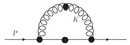
Figure 2: NLO HTL-summed quark self-energy $\Sigma_{1}^{(1)}$. The large dots indicate HTL-dressed vertex functions and propagators. All momenta are soft.

The diagram in Fig. 2 writes as follows:

$$\Sigma_{1}^{(1)}\left(P\right)=-ig^{2}C_{F}\int\frac{d^{4}K}{\left(2\pi\right)^{4}}\,\Gamma^{\mu}\left(P,Q\right)\Delta\left(Q\right)\Gamma^{\nu}\left(Q,P\right)\Delta_{\mu\nu}\left(K\right),$$ (17)

with $Q=P-K$, and the diagram in Fig. 3 writes as:

$$\Sigma_{2}^{(1)}\left(P\right)=\frac{-ig^{2}C_{F}}{2}\int\frac{d^{4}K}{\left(2\pi\right)^{4}}\mathbf{\,}\Gamma^{\mu\nu}\left(P,K\right)\Delta_{\mu\nu}\left(K\right).$$ (18)

There are three summation structures: Lorentz (explicit), Dirac, and RTF. We introduce now the Keldysh indices (“r/a” basis) of the closed-time-path (CTP) formulation of the finite-temperature real-time formalism keldysh ; real-time-formalism . The retarted (R), advanced (A), and symmetric (S) propagators are given by the following definitions:

$$\Delta_{B,F}^{\mathrm{R}}\left(K\right) \equiv \Delta_{B,F}^{\mathrm{ra}}\left(K\right)=\Delta_{B,F}\left(k_{0}+i\epsilon,\vec{k}\right);$$

$$\Delta_{B,F}^{\mathrm{A}}\left(K\right) \equiv \Delta_{B,F}^{\mathrm{ar}}\left(K\right)=\Delta_{B,F}\left(k_{0}-i\epsilon,\vec{k}\right);$$

$$\Delta_{B,F}^{\mathrm{S}}\left(K\right) \equiv \Delta_{B,F}^{\mathrm{rr}}\left(K\right)=N_{B,F}\left(k_{0}\right)\,\mathrm{sign}(k_{0})\left[\Delta_{B,F}^{\mathrm{R}}\left(K\right)-\Delta_{B,F}^{\mathrm{A}}\left(K\right)\right],$$ (19)

where $B$ stands for bosons and $F$ for fermions, and $N_{B,F}$ are related to the Bose-Einstein Fermi-Dirac distributions $n_{B,F}$ via the relations:

$$N_{B,F}\left(x\right)=1\pm 2n_{B,F}\left(x\right);\quad n_{B,F}\left(x\right)=\frac{1}{e^{\lvert x\rvert/T}\mp 1}.$$ (20)

We then have for the two components of $\Sigma_{1}^{(1)}$ the following explicit expressions:

$$\Sigma_{1\pm}^{(1)}\left(P\right) = \frac{-ig^{2}C_{F}}{2}\int\frac{d^{4}K}{\left(2\pi\right)^{4}}\mathbf{tr}\mathrm{\,}\gamma_{\pm p}\left[\Gamma_{\mathrm{arr}}^{\mu}\left(P,Q\right)\Delta^{\mathrm{R}}\left(Q\right)\Gamma_{\mathrm{arr}}^{\nu}\left(Q,P\right)\Delta_{\mu\nu}^{\mathrm{S}}\left(K\right)\right.$$ (21)

$$+\Gamma_{\mathrm{arr}}^{\mu}\left(P,Q\right)\Delta^{\mathrm{S}}\left(Q\right)\Gamma_{\mathrm{rar}}^{\nu}\left(Q,P\right)\Delta_{\mu\nu}^{\mathrm{A}}\left(K\right)$$

$$+\Gamma_{\mathrm{arr}}^{\mu}\left(P,Q\right)\Delta^{\mathrm{R}}\left(Q\right)\Gamma_{\mathrm{aar}}^{\nu}\left(Q,P\right)\Delta_{\mu\nu}^{\mathrm{A}}\left(K\right)$$

$$+\Gamma_{\mathrm{aar}}^{\mu}\left(P,Q\right)\Delta^{\mathrm{R}}\left(Q\right)\Gamma_{\mathrm{arr}}^{\nu}\left(Q,P\right)\Delta_{\mu\nu}^{\mathrm{R}}\left(K\right)$$

$$+\left.\Gamma_{\mathrm{ara}}^{\mu}\left(P,Q\right)\Delta^{\mathrm{A}}\left(Q\right)\Gamma_{\mathrm{rar}}^{\nu}\left(Q,P\right)\Delta_{\mu\nu}^{\mathrm{A}}\left(K\right)\right],$$

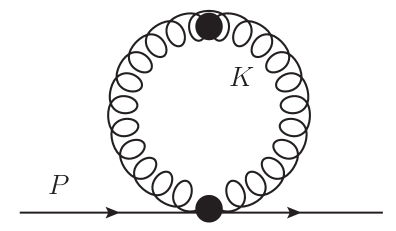
Figure 3: NLO HTL-summed quark self-energy $\Sigma_{1}^{(2)}$. The large dots indicate HTL-dressed vertex functions and propagators. All momenta are soft.

and for the two components of $\Sigma_{2}^{(1)}$ the following expressions:

$$\Sigma_{2\pm}^{(1)}\left(P\right) = \frac{-ig^{2}C_{F}}{4}\int\frac{d^{4}K}{\left(2\pi\right)^{4}}\mathbf{tr}\,\gamma_{\pm p}\left[\Gamma_{\mathrm{arrr}}^{\mu\nu}\left(P,K\right)\Delta_{\mu\nu}^{\mathrm{S}}\left(K\right)\right.$$ (22)

$$+\left.\Gamma_{\mathrm{aarr}}^{\mu\nu}\left(P,K\right)\Delta_{\mu\nu}^{\mathrm{R}}\left(K\right)+\Gamma_{\mathrm{arar}}^{\mu\nu}\left(P,K\right)\Delta_{\mu\nu}^{\mathrm{A}}\left(K\right)\right].$$

Note that these expressions of $\Sigma_{1\pm}^{(1)}$ in Eq. (21) and $\Sigma_{2}^{(1)}$ in Eq. (22) have been written in carrington–PRD75-2007-045019 using a different notation.

The HTL-dressed vertex functions $\Gamma$ are derived in the literature defu-heinz–EPJC7-1999-101 ; defu-et-al–PRD61-2000-085013 ; fueki-nakkagawa-yokota-yoshida . However, there are discrepancies in these results defu-et-al–PRD61-2000-085013 ; fueki-nakkagawa-yokota-yoshida , which led us to rederive all three and four-point HTL-dressed vertex functions ab initio in the CTP formalism. We recover the results of fueki-nakkagawa-yokota-yoshida ; these are presented in appendix A. For our needs, we have:

$$\Gamma_{\mathrm{arr}}^{\mu}\left(P,Q\right) = \gamma^{\mu}+I_{--}^{\mu}\left(P,Q\right);$$

$$\Gamma_{\mathrm{rar}}^{\mu}\left(P,Q\right) = \gamma^{\mu}+I_{+-}^{\mu}\left(P,Q\right);$$

$$\Gamma_{\mathrm{aar}}^{\mu}\left(P,Q\right) = \Gamma_{\mathrm{ara}}^{\mu}\left(P,Q\right)=0,$$ (23)

for the two-quarks-one-gluon vertices, and:

$$\Gamma_{\mathrm{arrr}}^{\mu\nu}\left(P,K\right)=I_{--}^{\mu\nu}\left(P,K\right);\quad\Gamma_{\mathrm{aarr}}^{\mu\nu}\left(P,K\right)=\Gamma_{\mathrm{arar}}^{\mu\nu}\left(P,K\right)=0,$$ (24)

for the two-quarks-two-gluons vertices. In these relations, the quantities $I$’s are hard thermal loops given by these solid-angle integrals:

$$I_{\eta_{1}\eta_{2}}^{\mu}\left(P,Q\right) = m_{f}^{2}\int\frac{d\Omega_{s}}{4\pi}\frac{S^{\mu}S/}{\left(PS+i\eta_{1}\epsilon\right)\left(QS+i\eta_{2}\epsilon\right)};$$

$$I_{\eta_{1}\eta_{2}}^{\mu\nu}\left(P,K\right) = m_{f}^{2}\int\frac{d\Omega_{s}}{4\pi}\frac{-S^{\mu}S^{\nu}S/}{\left(PS+i\eta_{1}\epsilon\right)\left(PS+i\eta_{2}\epsilon\right)}$$ (25)

$$\times\left[\frac{1}{\left(P+K\right)S+i\eta_{1}\epsilon}+\frac{1}{\left(P-K\right)S+i\eta_{2}\epsilon}\right],$$

where $S\equiv\left(1,\hat{s}\right)$ and the indices $\eta_{1}$ and $\eta_{2}$ take the values $+$ or $-$. Using these results, we can rewrite $\Sigma_{1\pm}^{(1)}$ and $\Sigma_{2\pm}^{(1)}$ above as simply:

$$\Sigma_{1\pm}^{(1)}\left(P\right) = \frac{-ig^{2}C_{F}}{2}\int\frac{d^{4}K}{\left(2\pi\right)^{4}}\mathbf{tr}\mathrm{\,}\gamma_{\pm p}\left[\left(\gamma^{\mu}+I_{--}^{\mu}\left(P,Q\right)\right)\Delta^{\mathrm{R}}\left(Q\right)\left(\gamma^{\nu}+I_{--}^{\nu}\left(Q,P\right)\right)\Delta_{\mu\nu}^{\mathrm{S}}\left(K\right)\right.$$ (26)

$$+\left(\gamma^{\mu}+I_{--}^{\mu}\left(P,Q\right)\right)\Delta^{\mathrm{S}}\left(Q\right)\left(\gamma^{\nu}+I_{+-}^{\nu}\left(Q,P\right)\right)\Delta_{\mu\nu}^{\mathrm{A}}\left(K\right);$$

$$\Sigma_{2\pm}^{(1)}\left(P\right) = \frac{-ig^{2}C_{F}}{4}\int\frac{d^{4}K}{\left(2\pi\right)^{4}}\mathbf{tr}\,\gamma_{\pm p}I_{--}^{\mu\nu}\left(P,K\right)\Delta_{\mu\nu}^{\mathrm{S}}\left(K\right).$$ (27)

We now work out the contractions over the Dirac and Lorentz indices. Starting with $\Sigma^{(1)}$, the contributions that do not include a hard thermal loop write generically as:

$$F_{\epsilon_{p};0}^{\mathrm{XY}}\left(P,K\right) \equiv \mathbf{tr}\left(\gamma_{\epsilon_{p}}\gamma^{\mu}\gamma_{\epsilon_{q}}\gamma^{\nu}\right)\Delta_{\mu\nu}^{\mathrm{X}}\left(K\right)\Delta_{-\epsilon_{q}}^{\mathrm{Y}}\left(Q\right)$$ (28)

$$= -2\left(1-\hat{p}_{\epsilon}.\hat{k}\,\hat{q}_{\epsilon}.\hat{k}\right)\Delta_{T}^{\mathrm{X}}\left(K\right)\Delta_{-\epsilon_{q}}^{\mathrm{Y}}\left(Q\right)$$

$$-\left[k_{0}^{2}\left(1-\left(\hat{p}_{\epsilon}.\hat{q}_{\epsilon}-2\hat{p}_{\epsilon}.\hat{k}\,\hat{q}_{\epsilon}.\hat{k}\right)\right)-2k_{0}k\right.$$

$$\left.\times\left(\hat{p}_{\epsilon}.\hat{k}+\hat{q}_{\epsilon}.\hat{k}\right)+k^{2}\left(1+\hat{p}_{\epsilon}.\hat{q}_{\epsilon}\right)\right]\tilde{\Delta}_{L}^{\mathrm{X}}\left(K\right)\Delta_{-\epsilon_{q}}^{\mathrm{Y}}\left(Q\right).$$

In this expression, $\tilde{\Delta}_{L}\left(K\right)=\Delta_{L}\left(K\right)/K^{2}$. Also, $\hat{p}_{\epsilon}=\epsilon_{p}\hat{p}$ with $\epsilon_{p}=\pm$ and similarly for $\hat{q}_{\epsilon}$, with summation understood over $\epsilon_{q}$. The superscripts X and Y indicate the RTF indices (R, S, and A). The contributions that involve one hard thermal loop vertex function writes:

$$F_{\epsilon_{p};\eta_{1}\eta_{2}}^{\mathrm{XY}}\left(P,K\right) \equiv \mathbf{tr}\left(\gamma_{\epsilon_{p}}I_{\eta_{1}\eta_{2}}^{\mu}\gamma_{\epsilon_{q}}\gamma^{\nu}\right)\Delta_{\mu\nu}^{\mathrm{X}}\left(K\right)\Delta_{-\epsilon_{q}}^{\mathrm{Y}}\left(Q\right)=m_{f}^{2}\int\frac{d\Omega_{s}}{4\pi}\frac{1}{\left(PS+i\eta_{1}\varepsilon\right)\left(QS+i\eta_{2}\varepsilon\right)}$$

$$\times\left[\left(1-\hat{p}_{\epsilon}.\hat{q}_{\epsilon}-\hat{p}_{\epsilon}.\hat{s}-\hat{q}_{\epsilon}.\hat{s}+\hat{p}_{\epsilon}.\hat{k}\,\hat{k}.\hat{s}+\hat{q}_{\epsilon}.\hat{k}\,\hat{k}.\hat{s}-\hat{k}.\hat{s}^{2}+\hat{p}_{\epsilon}.\hat{q}_{\epsilon}\hat{k}.\hat{s}^{2}+2\hat{p}_{\epsilon}.\hat{s}\,\hat{q}_{\epsilon}.\hat{s}\right.\right.$$

$$\left.-\hat{p}_{\epsilon}.\hat{k}\,\hat{q}_{\epsilon}.\hat{s}\,\hat{k}.\hat{s}-\hat{q}_{\epsilon}.\hat{k}\,\hat{p}_{\epsilon}.\hat{s}\,\hat{k}.\hat{s}\right)\Delta_{T}^{\mathrm{X}}\left(K\right)\Delta_{-\epsilon_{q}}^{\mathrm{Y}}\left(Q\right)-\left(k^{2}\left(1+\hat{p}_{\epsilon}.\hat{q}_{\epsilon}-\hat{p}_{\epsilon}.\hat{s}-\hat{q}_{\epsilon}.\hat{s}\right)\right.$$

$$-k_{0}k\left(\hat{p}_{\epsilon}.\hat{k}\,+\hat{q}_{\epsilon}.\hat{k}+2\hat{p}_{\epsilon}.\hat{q}_{\epsilon}\hat{k}.\hat{s}-\hat{q}_{\epsilon}.\hat{k}\,\hat{p}_{\epsilon}.\hat{s}-\hat{p}_{\epsilon}.\hat{k}\,\hat{q}_{\epsilon}.\hat{s}-\hat{q}_{\epsilon}.\hat{s}\,\hat{k}.\hat{s}-\hat{p}_{\epsilon}.\hat{s}\,\hat{k}.\hat{s}\right)$$

$$\left.\left.+k_{0}^{2}\left(\hat{p}_{\epsilon}.\hat{k}\,\hat{k}.\hat{s}+\hat{q}_{\epsilon}.\hat{k}\,\hat{k}.\hat{s}-\hat{k}.\hat{s}^{2}+\hat{p}_{\epsilon}.\hat{q}_{\epsilon}\hat{k}.\hat{s}^{2}-\hat{p}_{\epsilon}.\hat{k}\,\hat{q}_{\epsilon}.\hat{s}\,\hat{k}.\hat{s}-\hat{q}_{\epsilon}.\hat{k}\,\hat{p}_{\epsilon}.\hat{s}\,\hat{k}.\hat{s}\right)\right)\tilde{\Delta}_{L}^{\mathrm{X}}\left(K\right)\Delta_{-\epsilon_{q}}^{\mathrm{Y}}\left(Q\right)\right].$$

Here $\eta_{1}$ and $\eta_{2}$ take the values $\pm$. Due to the symmetry in $\Delta_{\mu\nu}$, The other contribution with one hard-thermal-loop vertex function is equal to the one above when changing $\eta_{1}$ into $\eta_{2}$, namely:

$$\mathbf{tr}\left(\gamma_{\epsilon_{p}}\gamma^{\mu}\gamma_{\epsilon_{q}}I_{\eta_{1}\eta_{2}}^{\nu}\right)\Delta_{\mu\nu}^{\mathrm{X}}\left(K\right)\Delta_{-\epsilon_{q}}^{\mathrm{Y}}\left(Q\right)=\mathbf{tr}\left(\gamma_{\epsilon_{p}}I_{\eta_{2}\eta_{1}}^{\mu}\gamma_{\epsilon_{q}}\gamma^{\nu}\right)\Delta_{\mu\nu}^{\mathrm{X}}\left(K\right)\Delta_{-\epsilon_{q}}^{\mathrm{Y}}\left(Q\right).$$ (30)

The contribution involving two hard-thermal-loop vertex functions is longer. It generically writes:

$$F_{\epsilon_{p};\eta_{1}\eta_{2};\eta_{1}^{\prime}\eta_{2}^{\prime}}^{\mathrm{XY}}\left(P,K\right) \equiv \mathbf{tr}\left(\gamma_{\epsilon_{p}}I_{\eta_{1}\eta_{2}}^{\mu}\gamma_{\epsilon_{q}}I_{\eta_{1}^{\prime}\eta_{2}^{\prime}}^{\nu}\right)\Delta_{\mu\nu}^{\mathrm{\ X}}\left(K\right)\Delta_{-\epsilon_{q}}^{\mathrm{Y}}\left(Q\right)$$

$$= m_{f}^{4}\int\frac{d\Omega_{s}}{4\pi}\frac{1}{\left(PS+i\eta_{1}\varepsilon\right)\left(QS+i\eta_{2}\varepsilon\right)}$$

$$\times\int\frac{d\Omega_{s^{\prime}}}{4\pi}\frac{1}{\left(PS^{\prime}+i\eta_{2}^{\prime}\varepsilon\right)\left(QS^{\prime}+i\eta_{1}^{\prime}\varepsilon\right)}\left[\left(-\hat{s}.\hat{s}^{\prime}-\hat{p}_{\epsilon}.\hat{q}_{\epsilon}\hat{s}.\hat{s}^{\prime}+\hat{p}_{\epsilon}.\hat{s}\,\hat{s}.\hat{s}^{\prime}+\hat{q}_{\epsilon}.\hat{s}\,\hat{s}.\hat{s}^{\prime}+\hat{p}_{\epsilon}.\hat{s}^{\prime}\,\hat{s}.\hat{s}^{\prime}\right.\right.$$

$$+\hat{q}_{\epsilon}.\hat{s}^{\prime}\,\hat{s}.\hat{s}^{\prime}-\hat{p}_{\epsilon}.\hat{s}\,\hat{q}_{\epsilon}.\hat{s}^{\prime}\,\hat{s}.\hat{s}^{\prime}-\hat{q}_{\epsilon}.\hat{s}\,\hat{p}_{\epsilon}.\hat{s}^{\prime}\,\hat{s}.\hat{s}^{\prime}-\hat{s}.\hat{s}^{\prime 2}+\hat{p}_{\epsilon}.\hat{q}_{\epsilon}\hat{s}.\hat{s}^{\prime 2}+\hat{k}.\hat{s}\,\hat{k}.\hat{s}^{\prime}+\hat{p}_{\epsilon}.\hat{q}_{\epsilon}\hat{k}.\hat{s}\,\hat{k}.\hat{s}^{\prime}$$

$$-\hat{p}_{\epsilon}.\hat{s}\,\hat{k}.\hat{s}\,\hat{k}.\hat{s}^{\prime}-\hat{q}_{\epsilon}.\hat{s}\,\hat{k}.\hat{s}\,\hat{k}.\hat{s}^{\prime}-\hat{p}_{\epsilon}.\hat{s}^{\prime}\hat{k}.\hat{s}\,\hat{k}.\hat{s}^{\prime}-\hat{q}_{\epsilon}.\hat{s}^{\prime}\hat{k}.\hat{s}\,\hat{k}.\hat{s}^{\prime}+\hat{p}_{\epsilon}.\hat{s}\,\hat{q}_{\epsilon}.\hat{s}^{\prime}\hat{k}.\hat{s}\,\hat{k}.\hat{s}^{\prime}$$

$$\left.+\hat{q}_{\epsilon}.\hat{s}\,\hat{p}_{\epsilon}.\hat{s}^{\prime}\hat{k}.\hat{s}\,\hat{k}.\hat{s}^{\prime}+\hat{s}.\hat{s}^{\prime}\hat{k}.\hat{s}\,\hat{k}.\hat{s}^{\prime}-\hat{p}_{\epsilon}.\hat{q}_{\epsilon}\hat{s}.\hat{s}^{\prime}\hat{k}.\hat{s}\,\hat{k}.\hat{s}^{\prime}\right)\Delta_{T}^{\mathrm{X}}\left(K\right)\Delta_{-\epsilon_{q}}^{\mathrm{Y}}\left(Q\right)$$

$$-\left[k^{2}\left(1+\hat{p}_{\epsilon}.\hat{q}_{\epsilon}-\hat{p}_{\epsilon}.\hat{s}-\hat{q}_{\epsilon}.\hat{s}-\hat{p}_{\epsilon}.\hat{s}^{\prime}-\hat{q}_{\epsilon}.\hat{s}^{\prime}+\hat{p}_{\epsilon}.\hat{s}\,\hat{q}_{\epsilon}.\hat{s}^{\prime}+\hat{q}_{\epsilon}.\hat{s}\,\hat{p}_{\epsilon}.\hat{s}^{\prime}+\hat{s}.\hat{s}^{\prime}-\hat{p}_{\epsilon}.\hat{q}_{\epsilon}\hat{s}.\hat{s}^{\prime}\right)\right.$$

$$-k_{0}k\left(\hat{k}.\hat{s}+\hat{k}.\hat{s}^{\prime}+\hat{p}_{\epsilon}.\hat{q}_{\epsilon}\,\hat{k}.\hat{s}+\hat{p}_{\epsilon}.\hat{q}_{\epsilon}\,\hat{k}.\hat{s}^{\prime}-\hat{p}_{\epsilon}.\hat{s}\,\hat{k}.\hat{s}-\hat{p}_{\epsilon}.\hat{s}\,\hat{k}.\hat{s}^{\prime}-\hat{q}_{\epsilon}.\hat{s}\,\hat{k}.\hat{s}-\hat{q}_{\epsilon}.\hat{s}\,\hat{k}.\hat{s}^{\prime}\right.$$

$$-\hat{p}_{\epsilon}.\hat{s}^{\prime}\,\hat{k}.\hat{s}-\hat{p}_{\epsilon}.\hat{s}^{\prime}\,\hat{k}.\hat{s}^{\prime}-\hat{q}_{\epsilon}.\hat{s}^{\prime}\,\hat{k}.\hat{s}-\hat{q}_{\epsilon}.\hat{s}^{\prime}\,\hat{k}.\hat{s}^{\prime}+\hat{p}_{\epsilon}.\hat{s}\,\hat{q}_{\epsilon}.\hat{s}^{\prime}\,\hat{k}.\hat{s}+\hat{p}_{\epsilon}.\hat{s}\,\hat{q}_{\epsilon}.\hat{s}^{\prime}\,\hat{k}.\hat{s}^{\prime}$$

$$\left.+\hat{q}_{\epsilon}.\hat{s}\,\hat{p}_{\epsilon}.\hat{s}^{\prime}\,\hat{k}.\hat{s}+\hat{q}_{\epsilon}.\hat{s}\,\hat{p}_{\epsilon}.\hat{s}^{\prime}\,\hat{k}.\hat{s}^{\prime}+\hat{k}.\hat{s}\,\hat{s}.\hat{s}^{\prime}+\hat{k}.\hat{s}^{\prime}\,\hat{s}.\hat{s}^{\prime}-\hat{p}_{\epsilon}.\hat{q}_{\epsilon}\hat{k}.\hat{s}\,\hat{s}.\hat{s}^{\prime}-\hat{p}_{\epsilon}.\hat{q}_{\epsilon}\hat{k}.\hat{s}^{\prime}\,\hat{s}.\hat{s}^{\prime}\right)$$

$$+k_{0}^{2}\left(\hat{k}.\hat{s}\,\hat{k}.\hat{s}^{\prime}+\hat{p}_{\epsilon}.\hat{q}_{\epsilon}\hat{k}.\hat{s}\,\hat{k}.\hat{s}^{\prime}-\hat{p}_{\epsilon}.\hat{s}\,\hat{k}.\hat{s}\,\hat{k}.\hat{s}^{\prime}-\hat{q}_{\epsilon}.\hat{s}\,\hat{k}.\hat{s}\,\hat{k}.\hat{s}^{\prime}-\hat{p}_{\epsilon}.\hat{s}^{\prime}\,\hat{k}.\hat{s}\,\hat{k}.\hat{s}^{\prime}-\hat{q}_{\epsilon}.\hat{s}^{\prime}\,\hat{k}.\hat{s}\,\hat{k}.\hat{s}^{\prime}\right.$$

$$\left.\left.\left.+\hat{p}_{\epsilon}.\hat{s}\,\hat{q}_{\epsilon}.\hat{s}^{\prime}\,\hat{k}.\hat{s}\,\hat{k}.\hat{s}^{\prime}+\hat{q}_{\epsilon}.\hat{s}\,\hat{p}_{\epsilon}.\hat{s}^{\prime}\,\hat{k}.\hat{s}\,\hat{k}.\hat{s}^{\prime}+\hat{k}.\hat{s}\,\hat{k}.\hat{s}^{\prime}\,\hat{s}.\hat{s}^{\prime}+\hat{p}_{\epsilon}.\hat{q}_{\epsilon}\hat{k}.\hat{s}\,\hat{k}.\hat{s}^{\prime}\,\hat{s}.\hat{s}^{\prime}\right)\right]\tilde{\Delta}_{L}^{\mathrm{X}}\left(K\right)\Delta_{-\epsilon_{q}}^{\mathrm{Y}}\left(Q\right)\right].$$

The integrand in $\Sigma_{2}^{\left(1\right)}$ is faster to write:

$$G_{\epsilon_{p};\eta_{1}\eta_{2}}^{\mathrm{X}}\left(P,K\right) \equiv \frac{1}{2}\mathbf{tr}\left(\gamma_{\epsilon_{p}}I_{\eta_{1}\eta_{2}}^{\mu\nu}\right)\Delta_{\mu\nu}^{\mathrm{X}}\left(K\right)=m_{f}^{2}\int\frac{d\Omega_{s}}{4\pi}\frac{1}{\left[PS+i\eta_{1}\varepsilon\right]\left[PS+i\eta_{2}\varepsilon\right]}$$

$$\times\left[\frac{1}{\left(P+K\right)S+i\eta_{1}\varepsilon}+\frac{1}{\left(P-K\right)S+i\eta_{2}\varepsilon}\right]$$

$$\times\left(1-\hat{p}_{\epsilon}.\hat{s}-\hat{k}.\hat{s}^{2}+\hat{p}_{\epsilon}.\hat{s}\,\hat{k}.\hat{s}^{2}\right)\Delta_{T}^{\mathrm{X}}\left(K\right)$$

$$\left(k^{2}\left(1-\hat{p}_{\epsilon}.\hat{s}\right)-2k_{0}k\left(\hat{k}.\hat{s}-\hat{p}_{\epsilon}.\hat{s}\,\hat{k}.\hat{s}\right)+k_{0}^{2}\,\hat{p}_{\epsilon}.\hat{s}\,\hat{k}.\hat{s}^{2}\right)\tilde{\Delta}_{L}^{\mathrm{X}}\left(K\right).$$

From these expressions, we can write the NLO HTL-dresses quark self-energy in a compact form:

$$\Sigma_{\pm}^{(1)}\left(P\right) = \frac{-ig^{2}C_{F}}{2}\int\frac{d^{4}K}{\left(2\pi\right)^{4}}\left[F_{\pm;0}^{\mathrm{SR}}\left(P,K\right)+F_{\pm;0}^{\mathrm{AS}}\left(P,K\right)+2F_{\pm;--}^{\mathrm{\ SR}}\left(P,K\right)+F_{\pm;--}^{\mathrm{AS}}\left(P,K\right)\right.$$ (33)

$$\left.+F_{\pm;-+}^{\mathrm{AS}}\left(P,K\right)+F_{\pm;--;--}^{\mathrm{SR}}\left(P,K\right)+F_{\pm;--;+-}^{\mathrm{AS}}\left(P,K\right)+G_{\pm;--}^{\mathrm{S}}\left(P,K\right)\right].$$

IV HTL vertex functions and Feynman parametrization

The next step is to find a way to evaluate the solid-angle integrals involved in the hard-thermal-loop vertex functions. The way we do this is to rewrite these integrals using the Feynman parametrization. From Eqs. (III), (III), and (III) above, we see that we have two kinds of solid-angle integrals to deal with, namely:

$$J_{\eta_{1}\eta_{2}}^{\mu\alpha}\left(P,Q\right) = \int\frac{d\Omega_{s}}{4\pi}\frac{S^{\mu}S^{\alpha}}{\left[PS+i\eta_{1}\varepsilon\right]\left[QS+i\eta_{2}\varepsilon\right]};$$

$$I_{\eta_{1}\eta_{2}}^{\mu\nu\alpha}\left(P,K\right) = \int\frac{d\Omega_{s}}{4\pi}\frac{S^{\mu}S^{\nu}S^{\alpha}}{\left[PS+i\eta_{1}\varepsilon\right]\left[PS+i\eta_{2}\varepsilon\right]}$$ (34)

$$\times\left[\frac{1}{\left(P+K\right)S+i\eta_{1}\varepsilon}+\frac{1}{\left(P-K\right)S+i\eta_{2}\varepsilon}\right].$$

The simplest of all these integrals is the integral:

$$J_{\eta_{1}\eta_{2}}^{00}\left(P,Q\right)=\int\frac{d\Omega_{s}}{4\pi}\frac{1}{\left(PS+i\eta_{1}\varepsilon\right)\left(QS+i\eta_{2}\varepsilon\right)}.$$ (35)

Remember that $S$ is the 4-vector ($1,\hat{s})$ and the integration is over the solid angle of $\hat{s}$. Let us put aside the $i\varepsilon$ prescription for the moment. Using the Feynman parametrization:

$$\frac{1}{AB}=\int_{0}^{1}du\frac{1}{\left(Au+B\left(1-u\right)\right)^{2}},$$ (36)

we write:

$$J_{\eta_{1}\eta_{2}}^{00}\left(P,Q\right)=\int_{0}^{1}du\int\frac{d\Omega_{s}}{4\pi}\frac{1}{\left[\left(P-Ku\right)S\right]^{2}}=\int_{0}^{1}\frac{du}{\left(P-Ku\right)^{2}},$$ (37)

where $K=P-Q$. In this case, the integral over $u$ can be done formally to get:

$$J_{\eta_{1}\eta_{2}}^{00}\left(P,Q\right)=\frac{1}{2\sqrt{\Delta}}\ln\frac{\left(1-u_{1}\right)u_{2}}{\left(1-u_{2}\right)u_{1}},$$ (38)

with the notation $u_{1,2}=\left(PK\pm\sqrt{\Delta}\right)/K^{2}$ and $\Delta=PK^{2}-P^{2}K^{2}$. Noticing that $PS+i\eta_{1}\varepsilon=p_{0}+i\eta_{1}\varepsilon-\vec{p}.\hat{s}$, the reintroduction of the $i\varepsilon$’s in the final result (38) is a matter of shifting $p_{0}\rightarrow p_{0}+i\eta_{1}\varepsilon$ and $q_{0}\rightarrow q_{0}+i\eta_{2}\varepsilon$. This also applies to the two next integrals.

The next HTL vertex function to consider is the solid-angle integral:

$$J_{\eta_{1}\eta_{2}}^{0i}\left(P,Q\right)=\int\frac{d\Omega_{s}}{4\pi}\frac{\hat{s}^{i}}{\left(PS+i\eta_{1}\varepsilon\right)\left(QS+i\eta_{2}\varepsilon\right)}.$$ (39)

Using a Feynman parametrization and the notation $R=P-\left(P-Q\right)u$ in which $p_{0}$ and $q_{0}$ are redefined with the corresponding $i\varepsilon$’s, we obtain the result:

$$J_{\eta_{1}\eta_{2}}^{0i}\left(P,Q\right) = \frac{1}{2}\int_{0}^{1}du\frac{r^{i}}{r}\int_{-1}^{1}dx\frac{x}{\left(r_{0}-xr\right)^{2}}$$ (40)

$$= \int_{0}^{1}du\left[\frac{r_{0}}{r_{0}^{2}-r^{2}}-\frac{1}{2r}\ln\frac{r_{0}+r}{r_{0}-r}\right]\frac{r^{i}}{r^{2}}.$$

Little useful comes from pushing further the integration over $u$ as the final result will not have a reasonably simple formal expression; it is better to leave this expression as it is and let the integration over $u$ be done numerically. However, the Feynman parametrization is useful as it reduces the number of integrations to be performed from two (solid angle) to one (over $u$) or zero when this latter is explicitly feasible.

The third HTL-vertex solid-angle integral is:

$$J_{\eta_{1}\eta_{2}}^{ij}\left(P,Q\right)=\int\frac{d\Omega_{s}}{4\pi}\frac{\hat{s}^{i}\hat{s}^{j}}{\left(PS+i\eta_{1}\varepsilon\right)\left(QS+i\eta_{2}\varepsilon\right)}.$$ (41)

This solid-angle integral can be performed using the Feynman parametrization and, still with $R=P-\left(P-Q\right)u$, we have:

$$J_{\eta_{1}\eta_{2}}^{ij}\left(P,Q\right) = \int_{0}^{1}du\left(A_{\eta_{1}\eta_{2}}\delta^{ij}+B_{\eta_{1}\eta_{2}}\hat{r}^{i}\hat{r}^{j}\right);$$

$$A_{\eta_{1}\eta_{2}} = -\frac{1}{r^{2}}\left(1-\frac{r_{0}}{2r}\ln\frac{r_{0}+r}{r_{0}-r}\right);$$

$$B_{\eta_{1}\eta_{2}} = \frac{1}{r_{0}^{2}-r^{2}}+\frac{3}{r^{2}}\left(1-\frac{r_{0}}{2r}\ln\frac{r_{0}+r}{r_{0}-r}\right).$$ (42)

The integration over $u$ is left to be performed numerically.

The two-gluon-two-fermion HTL vertex function uses the Feynman integral:

$$\frac{1}{ABC}=2!\int_{0}^{1}du_{1}\int_{0}^{1}du_{2}\frac{u_{1}}{\left[\left(C-B\right)u_{1}u_{2}+\left(B-A\right)u_{1}+A\right]^{3}}.$$ (43)

Now calling $P_{1,2}\equiv\left(p_{0}+i\eta_{1,2}\varepsilon,\vec{p}\right)$, we rewrite:

$$I_{\eta_{1}\eta_{2}}^{\mu\nu\alpha}\left(P,K\right) = J_{\eta_{1}\eta_{2}}^{\mu\nu\alpha}\left(P,K\right)+J_{\eta_{2}\eta_{1}}^{\mu\nu\alpha}\left(P,-K\right);$$

$$J_{\eta_{1}\eta_{2}}^{\mu\nu\alpha}\left(P,K\right) = \int\frac{d\Omega_{s}}{4\pi}\frac{S^{\mu}S^{\nu}S^{\alpha}}{P_{1}S\,P_{2}S\,\left(P_{1}+K\right)S}.$$ (44)

Calling $C=\left(P_{1}+K\right)S$, $B=P_{1}S$, $A=P_{2}S$, and the four-vector $T\equiv u_{1}u_{2}K+u_{1}\left(P_{1}-P_{2}\right)+P_{2}$, with $t_{0}=u_{1}u_{2}k_{0}+iu_{1}\left(\eta_{1}-\eta_{2}\right)\varepsilon+p_{0}+i\eta_{2}\varepsilon$ and $\vec{t}=u_{1}u_{2}\vec{k}+\vec{p}$, we have:

$$J_{\eta_{1}\eta_{2}}^{\mu\nu\alpha}\left(P,K\right)=2\int_{0}^{1}du_{1}\,u_{1}\int_{0}^{1}du_{2}\int\frac{d\Omega_{s}}{4\pi}\frac{S^{\mu}S^{\nu}S^{\alpha}}{\left(t_{0}-\vec{t}.\hat{s}\right)^{3}}.$$ (45)

Since the quantity $J_{\eta_{1}\eta_{2}}^{\mu\nu\alpha}$ is fully symmetric in the Lorentz indices, we only need to find the $000$, $00i$, $0ij$, and $ijk$ components. We have:

$$J_{\eta_{1}\eta_{2}}^{000}\left(P,K\right) = 2\int_{0}^{1}du_{1}\,u_{1}\int_{0}^{1}du_{2}\int\frac{d\Omega_{s}}{4\pi}\frac{1}{\left(t_{0}-\vec{t}.\hat{s}\right)^{3}}$$ (46)

$$= 2\int_{0}^{1}du_{1}\,u_{1}\int_{0}^{1}du_{2}\frac{t_{0}}{\left(t_{0}^{2}-t^{2}\right)^{2}}.$$

Note that in this case, the Feynman parametrization does not reduce the number of integrations to perform. Yet, it still has an advantage over the original integration over the solid angle $\Omega_{s}$ of the original unit vector $\hat{s}$ as, cast this way, the subsequent integration over the azimuthal angle of $\hat{k}$ will now be trivial. The next solid-angle integral is:

$$J_{\eta_{1}\eta_{2}}^{00i}\left(P,K\right) = 2\int_{0}^{1}du_{1}\,u_{1}\int_{0}^{1}du_{2}\int\frac{d\Omega_{s}}{4\pi}\frac{\hat{s}^{i}}{\left(t_{0}-\vec{t}.\hat{s}\right)^{3}}$$ (47)

$$= 2\int_{0}^{1}du_{1}\,u_{1}\int_{0}^{1}du_{2}\frac{t^{i}}{\left(t_{0}^{2}-t^{2}\right)^{2}}.$$

The next solid-angle integral involves a symmetric rank-2 tensor structure:

$$J_{\eta_{1}\eta_{2}}^{0ij}\left(P,K\right) = 2\int_{0}^{1}du_{1}\,u_{1}\int_{0}^{1}du_{2}\int\frac{d\Omega_{s}}{4\pi}\frac{\hat{s}^{i}\hat{s}^{j}}{\left(t_{0}-\vec{t}.\hat{s}\right)^{3}}$$

$$= 2\int_{0}^{1}du_{1}\,u_{1}\int_{0}^{1}du_{2}\left(C_{\eta_{1}\eta_{2}}\delta^{ij}+D_{\eta_{1}\eta_{2}}\hat{t}^{i}\hat{t}^{j}\right);$$

$$C_{\eta_{1}\eta_{2}} = \frac{t_{0}}{2t^{2}\left(t_{0}^{2}-t^{2}\right)}-\frac{1}{4t^{3}}\ln\frac{t_{0}+t}{t_{0}-t};$$

$$D_{\eta_{1}\eta_{2}} = \frac{t_{0}\left(5t^{2}-3t_{0}^{2}\right)}{2t^{2}\left(t_{0}^{2}-t^{2}\right)^{2}}+\frac{3}{4t^{3}}\ln\frac{t_{0}+t}{t_{0}-t},$$ (48)

and the last solid-angle integral involves a completely symmetric rank-3 tensor structure:

$$J_{\eta_{1}\eta_{2}}^{ijk}\left(P,K\right) = 2\int_{0}^{1}du_{1}\,u_{1}\int_{0}^{1}du_{2}\int\frac{d\Omega_{s}}{4\pi}\frac{\hat{s}^{i}\hat{s}^{j}\hat{s}^{k}}{\left(t_{0}-\vec{t}.\hat{s}\right)^{3}}$$

$$= 2\int_{0}^{1}du_{1}\,u_{1}\int_{0}^{1}du_{2}\left[E_{\eta_{1}\eta_{2}}\left(\hat{t}^{i}\delta^{jk}+\hat{t}^{j}\delta^{ki}+\hat{t}^{k}\delta^{ij}\right)+F_{\eta_{1}\eta_{2}}\hat{t}^{i}\hat{t}^{j}\hat{t}^{k}\right];$$

$$E_{\eta_{1}\eta_{2}} = \frac{1}{2t^{3}}\left(2+\frac{t_{0}^{2}}{\left(t_{0}^{2}-t^{2}\right)}-\frac{3t_{0}}{2t}\ln\frac{t_{0}+t}{t_{0}-t}\right);$$

$$F_{\eta_{1}\eta_{2}} = \frac{t}{\left(t_{0}^{2}-t^{2}\right)^{2}}-\frac{5}{2t^{3}}\left(2+\frac{t_{0}^{2}}{\left(t_{0}^{2}-t^{2}\right)}-\frac{3t_{0}}{2t}\ln\frac{t_{0}+t}{t_{0}-t}\right).$$ (49)

V Integration: A prototype

The next task is of course to evaluate all the integrals in Eq. (33), one after the other, and add them together. This is not an easy matter. Here we show how one can carry out with such expressions. We work in units of the quark thermal mass, i.e., we take $m_{f}=1$. This means that the ratio:

$$\frac{m_{g}^{2}}{m_{f}^{2}}=\frac{16N_{c}\left(N_{c}+N_{f}/2\right)}{6\left(N_{c}^{2}-1\right)}=\left(3+\frac{N_{f}}{2}\right),$$ (50)

with $N_{c}=3$ will replace $m_{g}^{2}$ in the gluon propagators. This ratio is equal to 4 for $N_{f}=2$, a value we take in this section.

It is best to work out a prototype, namely:

$$I\left(t,\varepsilon\right) = \int d^{4}K\Delta_{T}^{\mathrm{S}}\left(K\right)\Delta_{-}^{\mathrm{R}}\left(Q\right)\int\frac{d\Omega_{s}}{4\pi}\frac{1}{\left(PS-i\varepsilon\right)\left(QS-i\varepsilon\right)}$$ (51)

$$= \int_{0}^{+\infty}dk\int_{-1}^{+1}dx\int_{-\infty}^{+\infty}dk_{0}\int_{0}^{1}du\,M\left(t,k,k_{0},x,u,\varepsilon\right).$$

The notation is explained as we proceed. As before, $P=(p_{0},\vec{p})$ is the four-momentum of the external soft ”on-shell” quark, $K=(k_{0},\vec{k})$ the four-momentum of the soft gluon in the loop, and $Q=P-K$; see Fig. 2. The quantity $x$ is cosine the angle between $\vec{k}$ and $\vec{p}$ – the integration over the azimuthal angle of $\hat{k}$ is done trivially. The integration variable $u$ is from the Feynman parametrization when the solid-angle integral is performed, see Eq. (37). The quantity $t$ is the ratio $p/p_{0}$, to be introduced more naturally later in this discussion. The integrand $M$ in this example is therefore given by the following relation:

$$M\left(t,k,k_{0},x,u,\varepsilon\right)=\frac{k^{2}N_{B}\left(k_{0}\right)\mathrm{sign}\left(k_{0}\right)}{Fu^{2}+2Bu+A}\left[\Delta_{T}^{\mathrm{R}}\left(k,k_{0},\varepsilon\right)-\Delta_{T}^{\mathrm{R}}\left(k,k_{0},-\varepsilon\right)\right]\Delta_{-}^{\mathrm{R}}\left(q,q_{0},\varepsilon\right).$$ (52)

The quantity $N_{B}\left(k_{0}\right)$ is related to the Bose-Einstein distribution, see Eq. (20), and $\Delta_{T}^{\mathrm{R}}\left(k,k_{0},\varepsilon\right)$ is the retarded transverse gluon propagator, which can be written as:

$$\Delta_{T}^{\mathrm{R}(-1)}\left(k,k_{0},\varepsilon\right) = \frac{4k_{0}^{2}}{3k^{2}}+\left(k^{2}-k_{0}^{2}\right)\left[1-\frac{k_{0}}{3k^{3}}\ln\left(\frac{(k_{0}-k)^{2}+\varepsilon^{2}}{(k_{0}+k)^{2}+\varepsilon^{2}}\right)\right]$$

$$+\boldsymbol{i}\left[\frac{2k_{0}}{3k^{2}}\left(k_{0}^{2}-k^{2}\right)\left(\arctan\left(\frac{\varepsilon}{k_{0}-k}\right)-\arctan\left(\frac{\varepsilon}{k_{0}+k}\right)\right)-\varepsilon\,\mathrm{sign}\left(k_{0}\right)\right].$$

The quantity $\Delta_{-}^{\mathrm{R}}\left(q,q_{0},\varepsilon\right)$ is the retarted quark propagator, given by:

$$\Delta_{-}^{\mathrm{R}\left(-1\right)}\left(q,q_{0},\varepsilon\right) = \frac{1}{q}+q-q_{0}-\frac{q_{0}-q}{4q^{2}}\ln\left(\frac{(q_{0}+q)^{2}+\varepsilon^{2}}{(q_{0}-q)^{2}+\varepsilon^{2}}\right)$$ (54)

$$+\frac{\varepsilon}{2q^{2}}\left[\arctan\left(\frac{\varepsilon}{q_{0}+q}\right)-\arctan\left(\frac{\varepsilon}{q_{0}-q}\right)\right]$$

$$-\boldsymbol{i}\left(\varepsilon+\frac{\varepsilon}{4q^{2}}\ln\left(\frac{(q_{0}+q)^{2}+\varepsilon^{2}}{(q_{0}-q)^{2}+\varepsilon^{2}}\right)\right.$$

$$+\left.\frac{q_{0}-q}{2q^{2}}\left[\arctan\left(\frac{\varepsilon}{q_{0}+q}\right)-\arctan\left(\frac{\varepsilon}{q_{0}-q}\right)\right]\right).$$

The momentum $\vec{q}=\vec{p}-\vec{k}$ and the energy $q_{0}=p_{0}-k_{0}$ where $p_{0}$ is the quark energy. The quantities $F$, $B$ and $A$ in the denominator of $M$ are regularized relativistic relations:

$$A = \left(p_{0}-i\varepsilon\right)^{2}-p^{2};$$

$$B = \vec{k}.\vec{p}-\left(k_{0}-2i\varepsilon\right)\left(p_{0}-i\varepsilon\right);$$

$$F = \left(k_{0}-2i\varepsilon\right)^{2}-k^{2}.$$ (55)

As mentioned above, the variable $t$ is the ratio $p/p_{0}$, in terms of which the quark momentum writes:

$$p\left(t\right)/m_{f}=\sqrt{\frac{t}{1-t}-\frac{1}{2}\ln\left(\frac{1+t}{1-t}\right)}.$$ (56)

Remember we take the quark thermal mass $m_{f}=1$. The above relation comes from the lowest-order quark dispersion relation $\Delta_{-}^{-1}(p_{0},p)=0$ where $\Delta_{-}^{-1}$ is given in Eq. (13). The behavior of $p(t)$ and $p_{0}(t)=\omega_{-}(p(t))$ is shown in Fig. 4. Slow-moving quarks would have $p\lesssim 1$ (in units of $m_{f}$), which translates into $t\lesssim 0.64$. The limit $t\rightarrow 1$ is the fast-moving region in which both $p(t)$ and $p_{0}(t)$ are large.

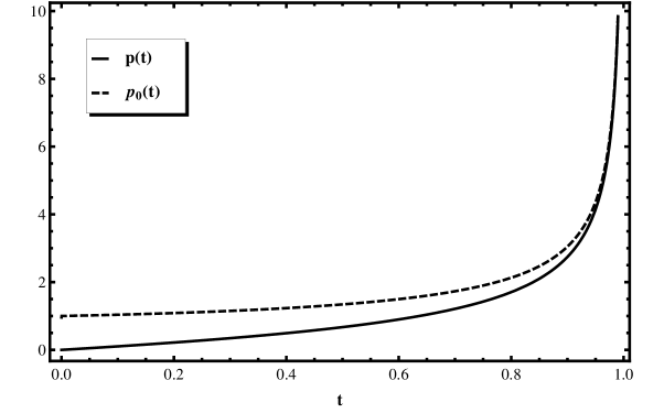
Figure 4: The quark momentum $p$ (solid) and energy $p_{0}$ (dashed) as functions of the ratio $t=p/p_{0}$. The quark mass $m_{f}$ is taken equal to one. The fast-moving limit is $t\rightarrow 1$. Slow-moving quarks would be for $t\lesssim 0.64$.

In this example, the integral over $u$ can be done analytically, which reduces the number of integrations in Eq. (51) to three. Indeed, one obtains:

$$I(t,\varepsilon) = \int_{0}^{+\infty}dk\int_{-1}^{+1}dx\int_{-\infty}^{+\infty}dk_{0}\,k^{2}N_{B}\left(k_{0}\right)\mathrm{sign}\left(k_{0}\right)$$ (57)

$$\times\left[\Delta_{T}^{\mathrm{R}}\left(k,k_{0},\varepsilon\right)-\Delta_{T}^{\mathrm{R}}\left(k,k_{0},-\varepsilon\right)\right]\Delta_{-}^{\mathrm{R}}\left(q,q_{0},\varepsilon\right)V\left(t,k,k_{0},x,\varepsilon\right),$$

with the function $V$ given by the following expression, see Eq. (38):

$$V\left(t,k,k_{0},x,\varepsilon\right) = \int_{0}^{1}du\frac{1}{Fu^{2}+2Bu+A}$$ (58)

$$= \frac{1}{2\sqrt{\Delta}}\left(\frac{1}{2}\ln\left[\frac{\left(\left(r_{1}-1\right)^{2}+i_{1}{}^{2}\right)\left(r_{2}{}^{2}+i_{2}{}^{2}\right)}{\left(\left(r_{2}-1\right)^{2}+i_{2}{}^{2}\right)\left(r_{1}^{2}+i_{1}{}^{2}\right)}\right]\right.$$

$$+\boldsymbol{i}\left[\arctan\left(\frac{r_{1}}{i_{1}}\right)-\arctan\left(\frac{r_{1}-1}{i_{1}}\right)\right.$$

$$\left.-\left.\arctan\left(\frac{r_{2}}{i_{2}}\right)+\arctan\left(\frac{r_{2}-1}{i_{2}}\right)\right]\right).$$

The quantities are $r_{i}=\mathop{\mathrm{R}e}s_{i}$ and $i_{i}=\mathop{\mathrm{I}m}s_{i}$ with:

$$s_{1}=\frac{-B+\sqrt{\Delta}}{F};\quad s_{2}=\frac{-B-\sqrt{\Delta}}{F};\quad\Delta=B^{2}-AF.$$ (59)

There are difficulties with the integral $I\left(t,\varepsilon\right)$. One is that the integrand features sudden jumps, those coming from the arctans in the propagators, the Bose-Einstein distribution at $k_{0}=0$, and eventually those coming from $V$. Such jumps make any integration method either too long to be useful, or give unstable results. This instability is more intense when trying to take $\varepsilon$ smaller and smaller. So, in order to see more closely what is at stake, we have partitioned the integration region in the $\left(k,k_{0}\right)$ plane into domains bounded by the following lines of sudden jumps:

$$k_{0} = 0;\quad k_{0}=\pm k;\quad k_{0}=p_{0}\pm\sqrt{p^{2}+k^{2}-2pkx};$$

$$k = k_{t}\equiv\frac{1}{2}\frac{p_{0}^{2}-p^{2}}{p_{0}-xp}=\frac{1}{2t}\frac{1-t^{2}}{1-xt}\sqrt{\frac{t}{1-t}-\frac{1}{2}\ln\left(\frac{1+t}{1-t}\right)}.$$ (60)

The last (vertical) line is simply the line $k=p_{0}-q$. Using the change of variables $\theta=\arctan k$ and $\phi=\arctan k_{0}$, these domains are plotted in Fig. 5.

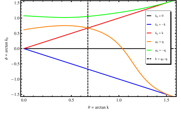
Figure 5: Boundaries in $\left(k,k_{0}\right)$ plane at which the integrand $M$ has sharp jumps (see text for details). Here $t=0.45$ and $x=0.8$.

If one integrates $M$ in each of the domains of Fig. 5 separately and sum up the results, one finds that $I\left(t,\varepsilon\right)$ becomes stable and reliable in the limit $\varepsilon\rightarrow 0$. See Fig. 6 (the units of $I(t,\varepsilon)$ there are arbitrary): both the real and imaginary parts of $I(t)$ behave smoothly, and these two plots are obtained with $\varepsilon=3.2\times 10^{-6}$ (in units of $m_{f}$).

Figure 6: The real and imaginary parts of $I(t)$ for soft $p$ (meaning $t\lesssim 0.64$). Both parts have a stable behavior. Here, $\varepsilon=3.2\times 10^{-6}$. The units of $I(t)$ are arbitrary.

The dependence in $\varepsilon$ is of course an issue to explore. Fig. 7 shows how for example $I(t=0.32,\varepsilon)$ behaves as a function of $m=-\log_{10}\varepsilon$.

Figure 7: The $\varepsilon$-dependence of $I(t)$. We see stability and convergence up until $\epsilon\simeq 10^{-8}$. Here $t=p/p_{0}$ is take equal to $0.32$.

The behavior is stable down until $\varepsilon\simeq 10^{-8}$ (in units of $m_{f}$), below which the numerics loose reliability. This is way beyond any precision we can hope for, and we notice that $I(t,\varepsilon)$ converges smoothly to a finite value already satisfactorily reached at $\varepsilon\simeq 10^{-6}$. The smooth convergence to finite values is also obtained for other values of $t$.

VI Outlook

The present work aims at calculating the energies and damping rates of slow-moving quarks at next-to-leading order in the context of massless QCD at high temperature using the real-time formulation of the fully-dressed hard-thermal-loop perturbative expansion. These quantities are extracted from the poles of the quark propagators. At lowest order, the energies $\omega_{\pm}\left(p\right)$ are real, see Eq. (11). The next-to-leading order contributions necessitate the determination of the next-to-leading order quark self-energies $\Sigma_{\pm}^{(1)}$, see Eq. (9).

In this work, we have given the analytic expression of $\Sigma_{\pm}^{(1)}$ in terms of loop-four-momentum integrals involving fully-HTL-dressed quark and gluon propagators and vertex functions, see Eqs. (21) and ( 22). These expressions were already written in carrington–PRD75-2007-045019 . The HTL vertex functions themselves are derived and written as solid-angle integrals. We have rewritten these latter using the Feynman parametrization in order to perform these solid-angle integrals.

The next step is to perform the integrals. This is done numerically. The usual approach is to use the spectral decomposition of the dressed propagators. But we refrain from doing so and will try to tackle these integrals head on. This is known to be difficult. One main difficulty is the jumps the integrands suffer from at the singular lines of the propagators, more prominently as the regularizer $\varepsilon\rightarrow 0$. We have used a prototype integral to indicate how such difficulties might be overcome. By splitting the integration region into appropriate domains, we can obtain an estimate of the prototype integral with a robust behavior down to $\epsilon\simeq 10^{-8}$ in unit of the quark thermal mass $m_{f}$.

Of course there are many other terms to handle, more involved than the prototype. Will there be stability for each? Can we add them all? This is currently under investigation.

Appendix A Hard Thermal Loop Dressed Vertex Functions

Discrepancies between different results in the literature defu-et-al–PRD61-2000-085013 ; fueki-nakkagawa-yokota-yoshida regarding the derivation of the three and four-point hard-thermal-loop vertex functions in the CTP formalism imposed on us an ab initio recalculation of these quantities. We recover the results of fueki-nakkagawa-yokota-yoshida . This appendix summarizes our steps, with a notation close to fueki-nakkagawa-yokota-yoshida .

A.1 Three-Point Vertex Functions

The quark-gluon vertex functions are the sum of the bare vertices and the corresponding hard thermal loops:

$$\Gamma^{\mu}=\gamma^{\mu}+\delta\Gamma^{\mu}.$$ (61)

In the {12} basis of the CTP formalism, the bare vertex $\gamma^{\mu}$ is given by the relations:

$$\gamma_{ijk}^{\mu}=\left\{\begin{tabular}[]{l}$\left(-1\right)^{i-1}\gamma^{\mu}\quad\mathrm{when}\quad i=j=k$\\ $0\quad\mathrm{otherwise}$\end{tabular}\right..$$ (62)

The indices $i$, $j$, and $k$ take the values 1 and 2. The hard-thermal-loop contributions $\delta\Gamma^{\mu}$ to these vertices are obtained by calculating the following one-loop diagrams:

$$\delta\Gamma_{ijk}^{\mu}\left(P,Q,R\right)=4ig^{2}C_{F}\int\frac{d^{4}K}{\left(2\pi\right)^{4}}K^{\mu}\leavevmode\hbox{\hbox to0.0pt{\thinspace/\hss}{$K$}}V_{ijk}^{\prime}-2ig^{2}N_{c}\int\frac{d^{4}K}{\left(2\pi\right)^{4}}K^{\mu}\leavevmode\hbox{\hbox to0.0pt{\thinspace/\hss}{$K$}}\left(V_{ijk}^{\prime}+V_{ijk}\right),$$ (63)

in which the loop momentum $K$ is hard, in front of which external momenta are neglected. In this expression,

$$V_{ijk} = \left(-1\right)^{i+j+k-3}\bar{D}_{ij}\left(K\right)D_{jk}\left(K-Q\right)D_{ki}\left(K+P\right);$$

$$V_{ijk}^{\prime} = \left(-1\right)^{i+j+k-3}D_{ij}\left(K\right)\bar{D}_{jk}\left(K-Q\right)\bar{D}_{ki}\left(K+P\right).$$ (64)

The functions $D_{ij}\left(K\right)$ are the four {12} components of the bare bosonic propagator:

$$D\left(K\right) = \begin{pmatrix}D_{11}\left(K\right)&D_{12}\left(K\right)\\ D_{21}\left(K\right)&D_{22}\left(K\right)\end{pmatrix}$$ (65)

$$= \begin{pmatrix}\frac{1+n_{B}\left(k_{0}\right)}{K^{2}+i\varepsilon}-\frac{n_{B}\left(k_{0}\right)}{K^{2}-i\varepsilon}&\frac{\theta\left(-k_{0}\right)+n_{B}\left(k_{0}\right)}{K^{2}+i\varepsilon}-\frac{\theta\left(-k_{0}\right)+n_{B}\left(k_{0}\right)}{K^{2}-i\varepsilon}\\ \frac{\theta\left(k_{0}\right)+n_{B}\left(k_{0}\right)}{K^{2}+i\varepsilon}-\frac{\theta\left(k_{0}\right)+n_{B}\left(k_{0}\right)}{K^{2}-i\varepsilon}&\frac{n_{B}\left(k_{0}\right)}{K^{2}+i\varepsilon}-\frac{1+n_{B}\left(k_{0}\right)}{K^{2}-i\varepsilon}\end{pmatrix}.$$

The quantity $\bar{D}_{ij}\left(K\right)$ is $D_{ij}\left(K\right)$ with $n_{B}\left(k_{0}\right)$ replaced by $-n_{F}\left(k_{0}\right)$. We write these quantities in terms of advanced ($A$), retarded ($R$) and symmetric ($F$) propagators:

$$D_{11} = \frac{1}{2}\left(F+A+R\right);\quad D_{12}=\frac{1}{2}\left(F+A-R\right);$$

$$D_{21} = \frac{1}{2}\left(F-A+R\right);\quad D_{22}=\frac{1}{2}\left(F-A-R\right),$$ (66)

where:

$$R\left(K\right) = \frac{\theta\left(k_{0}\right)}{K^{2}+i\varepsilon}+\frac{\theta\left(-k_{0}\right)}{K^{2}-i\varepsilon};$$

$$A\left(K\right) = \frac{\theta\left(-k_{0}\right)}{K^{2}+i\varepsilon}+\frac{\theta\left(k_{0}\right)}{K^{2}-i\varepsilon};$$

$$F\left(K\right) = \left(1\pm 2n_{B,F}\left(k_{0}\right)\right)\left(\frac{1}{K^{2}+i\varepsilon}-\frac{1}{K^{2}-i\varepsilon}\right).$$ (67)

The vertex functions in the {$RA$} basis are linearly related to the same functions defined in the {12} basis. For example, the three-point vertex function $\Gamma_{RAA}$ is given by the linear relation:

$$\Gamma_{RAA}=\Gamma_{111}+\Gamma_{112}+\Gamma_{121}+\Gamma_{122}.$$ (68)

This relation applies to the kernels $V$ and $V^{\prime}$. Using the expressions (64) of the functions $V$ and $V^{\prime}$, and the relations (66), we arrive at the following expression:

$$V_{RAA}=\frac{1}{2}(A_{1}A_{2}A_{3}+R_{1}R_{2}R_{3}+F_{1}A_{2}A_{3}+R_{1}F_{2}A_{3}+R_{1}R_{2}F_{3}),$$ (69)

where, for short, 1, 2 and 3 denote the arguments $K$, $K-Q$ and $K+P$ respectively. Next is to integrate over the internal momentum $K$. This is performed in two steps: first over $k_{0}$, done using the residue theorem in the $k_{0}$-complex plane. In this regard, the terms $A_{1}A_{2}A_{3}$ and $R_{1}R_{2}R_{3}$ give zero contribution each. The three others give the following contributions:

$$FAA = \frac{+i}{8\pi^{2}}\int_{0}^{+\infty}kdkN_{B,F}(k)\int\frac{d\Omega_{s}}{4\pi}\frac{S^{\mu}S/}{\left(PS-i\varepsilon\right)\left(QS+i\varepsilon\right)};$$

$$RFA = \frac{-i}{8\pi^{2}}\int_{0}^{+\infty}kdkN_{B,F}(k)\int\frac{d\Omega_{s}}{4\pi}\frac{S^{\mu}S/}{\left(QS+i\varepsilon\right)\left(\left(P+Q\right)S-i\varepsilon\right)};$$

$$RRF = \frac{-i}{8\pi^{2}}\int_{0}^{+\infty}kdkN_{B,F}(k)\int\frac{d\Omega_{s}}{4\pi}\frac{S^{\mu}S/}{\left(PS-i\varepsilon\right)\left(\left(P+Q\right)S-i\varepsilon\right)}.$$ (70)

Here, the quantities $N_{B,F}(k)$ are defined in Eq. (20) and $S=\left(1,\hat{s}\right)$ is a time-like unit four-vector in which $\hat{s}$ is nothing but $\vec{k}/k$. Remember that every external momentum is neglected in front of $K$. When summing the contributions together, some will add up to a product of propagator denominators multiplied by $i\varepsilon$, so are dropped, and some will stand. In the end, we find:

$$\delta\Gamma_{RAA}=\frac{-g^{2}C_{F}}{2\pi^{2}}\int_{0}^{+\infty}kdk\left(n_{B}\left(k\right)+n_{F}\left(k\right)\right)\int\frac{d\Omega}{4\pi}\frac{S^{\mu}S/}{\left(PS-i\varepsilon\right)\left(QS+i\varepsilon\right)}.$$ (71)

Now the integration over $k$ can be done. Using the known results:

$$\int_{0}^{+\infty}dkkn_{B}\left(k\right)=\frac{\pi^{2}}{6}T^{2};\quad\int_{0}^{+\infty}dkkn_{F}\left(k\right)=\frac{\pi^{2}}{12}T^{2},$$ (72)

we finally find the expression for this hard thermal loop:

$$\delta\Gamma_{RAA}\left(P,Q,R\right)=-m_{f}^{2}\int\frac{d\Omega}{4\pi}\frac{S^{\mu}S/}{\left(PS-i\varepsilon\right)\left(QS+i\varepsilon\right)},$$ (73)

with $m_{f}=\sqrt{C_{F}/8}gT$. The other three-point HTL vertex functions are obtained following a similar procedure. The relations between vertices in the {RA} and {12} bases are:

$$\Gamma_{ARA} = \Gamma_{111}+\Gamma_{112}+\Gamma_{211}+\Gamma_{212};$$

$$\Gamma_{AAR} = \Gamma_{111}+\Gamma_{121}+\Gamma_{211}+\Gamma_{221};$$

$$\Gamma_{RRA} = \Gamma_{111}+\Gamma_{112}+\Gamma_{221}+\Gamma_{222};$$

$$\Gamma_{RAR} = \Gamma_{111}+\Gamma_{121}+\Gamma_{212}+\Gamma_{222};$$

$$\Gamma_{ARR} = \Gamma_{111}+\Gamma_{211}+\Gamma_{122}+\Gamma_{222};$$

$$\Gamma_{RRR} = \Gamma_{111}+\Gamma_{122}+\Gamma_{212}+\Gamma_{221},$$ (74)

with $\Gamma_{AAA}=0$ identically. For each of these vertex functions, one works out steps similar to the ones for $\Gamma_{RAA}$ and one finds:

$$\delta\Gamma_{ARA}\left(P,Q,R\right) = -m_{f}^{2}\int\frac{d\Omega_{s}}{4\pi}\frac{S^{\mu}S/}{\left(PS+i\varepsilon\right)\left(QS-i\varepsilon\right)};$$

$$\delta\Gamma_{AAR}\left(P,Q,R\right) = -m_{f}^{2}\int\frac{d\Omega_{s}}{4\pi}\frac{S^{\mu}S/}{\left(PS+i\varepsilon\right)\left(QS+i\varepsilon\right)};$$

$$\delta\Gamma_{RRR}\left(P,Q,R\right) = -m_{f}^{2}\int\frac{d\Omega_{s}}{4\pi}\frac{S^{\mu}S/}{\left(PS-i\varepsilon\right)\left(QS-i\varepsilon\right)};$$

$$\delta\Gamma_{RRA}\left(P,Q,R\right) = \delta\Gamma_{RAR}\left(P,Q,R\right)=\delta\Gamma_{ARR}\left(P,Q,R\right)=0.$$ (75)

A.2 Four-Point Vertex Functions

The two-gluon-two-quark vertex functions are all hard thermal loops, no bare terms, given in the {12} basis by the relation:

$$\delta\Gamma_{ijkl}^{\mu\nu}\left(P,Q,R,U\right) = -8ig^{2}\left(-1\right)^{i+j+k+l}\int\frac{d^{4}K}{\left(2\pi\right)^{4}}K^{\mu}K^{\nu}\leavevmode\hbox{\hbox to0.0pt{\thinspace/\hss}{$K$}}$$ (76)

$$\times\left[C_{F}D_{ij}\left(K\right)\bar{D}_{jk}\left(K-Q\right)\bar{D}_{kl}\left(K+P+U\right)\bar{D}_{li}\left(K+P\right)\right.$$

$$-N_{c}\bar{D}_{ij}\left(K\right)D_{jk}\left(K-Q\right)D_{kl}\left(K+P+U\right)D_{li}\left(K+P\right)$$

$$\left.+\frac{1}{2}N_{c}D_{li}(K-P)D_{jl}(K-P-U)\bar{D}_{kj}(K+R)\bar{D}_{ik}(K)\right].$$

Consider for example the {$RA$}-component $\delta\Gamma_{RAAA}$, given by:

$$\delta\Gamma_{RAAA}=\delta\Gamma_{1111}+\delta\Gamma_{1112}+\delta\Gamma_{1121}+\delta\Gamma_{1211}+\delta\Gamma_{1122}+\delta\Gamma_{1212}+\delta\Gamma_{1221}+\delta\Gamma_{1222}.$$ (77)

Consider the term multiplying $C_{F}$ in Eq. (76) and call it $\delta\Gamma_{RAAA}^{1}$. Using the decompositions in Eq. ( 66), we obtain, in a similar symbolic notation as in Eq. (69), the relation:

$$\delta\Gamma_{RAAA}^{1}=\frac{1}{2}F_{1}A_{2}A_{3}A_{4}+\frac{1}{2}R_{1}F_{2}A_{3}A_{4}+\allowbreak\frac{1}{2}R_{1}R_{2}F_{3}A_{4}+\frac{1}{2}R_{1}R_{2}R_{3}F_{4}.$$ (78)

The subscripts 1,2,3, and 4 stand for the momenta $K$, $K-Q$, $K+P+U$, and $K+P$ respectively. The two contributions $\frac{1}{2}A_{1}A_{2}A_{3}A_{4}$ and $\frac{1}{2}R_{1}R_{2}R_{3}R_{4}$ to $\delta\Gamma_{RAAA}^{1}$ yield zero each in the $k_{0}$-complex-plane integration and are not displayed explicitly in Eq. (78). The different terms in Eq. (78) contribute as follows:

$$FAAA = \int_{0}^{+\infty}\frac{kdk}{16\pi^{2}}\int\frac{d\Omega_{s}}{4\pi}\frac{iN_{B}(k)S^{\mu}S^{\nu}S/}{\left(\left(2P+U\right)S+i\varepsilon\right)\left(\left(P-R\right)S+i\varepsilon\right)\left(PS+i\varepsilon\right)};$$

$$RFAA = \int_{0}^{+\infty}\frac{kdk}{16\pi^{2}}\int\frac{d\Omega_{s}}{4\pi}\frac{-iN_{B}(k)K^{\mu}K^{\nu}S/}{\left(\left(2P+U\right)S+i\varepsilon\right)\left(\left(R+P+U\right)S-i\varepsilon\right)\left(\left(P+U\right)S-i\varepsilon\right)};$$

$$RRFA = \int_{0}^{+\infty}\frac{kdk}{16\pi^{2}}\int\frac{d\Omega_{s}}{4\pi}\frac{iN_{F}(k)S^{\mu}S^{\nu}S/}{\left(\left(R-P\right)S-i\varepsilon\right)\left(\left(R+P+U\right)S-i\varepsilon\right)\left(RS+i\varepsilon\right)};$$

$$RRRF = \int_{0}^{+\infty}\frac{kdk}{16\pi^{2}}\int\frac{d\Omega_{s}}{4\pi}\frac{iN_{F}(k)S^{\mu}S^{\nu}S/}{\left(PS+i\varepsilon\right)\left(\left(P+U\right)S-i\varepsilon\right)\left(RS+i\varepsilon\right)}.$$ (79)

Adding these terms together yield the following result:

$$\delta\Gamma_{RAAA}^{1}=\frac{i}{8\pi^{2}}\int_{0}^{+\infty}kdk\int\frac{d\Omega_{s}}{4\pi}\frac{\left(n_{B}\left(k\right)+n_{F}\left(k\right)\right)S^{\mu}S^{\nu}S/}{\left(PS-i\varepsilon\right)\left(QS+i\varepsilon\right)\left(\left(P+U\right)S-i\varepsilon\right)}.$$ (80)

The integrations over $k$ can now be done using Eq. (72 ). The terms multiplying $N_{c}$ and $N_{c}/2$ in Eq. (76) are worked out in a similar way; they cancel each other. We therefore have the hard-thermal-loop four-vertex function:

$$\delta\Gamma_{RAAA}\left(P,Q,R,U\right) = m_{f}^{2}\int\frac{d\Omega_{s}}{4\pi}\frac{S^{\mu}S^{\nu}S/}{\left(PS-i\varepsilon\right)\left(QS+i\varepsilon\right)}$$ (81)

$$\times\left[\frac{1}{\left(\left(P+U\right)S-i\varepsilon\right)}+\frac{1}{\left(\left(P+R\right)S-i\varepsilon\right)}\right].$$

The other {$RA$} four-vertex hard thermal loops are worked out in a similar way. With $\delta\Gamma_{AAAA}=0$ and using the linear relationships:

$$\delta\Gamma_{ARAA} = \delta\Gamma_{1111}+\delta\Gamma_{1112}+\delta\Gamma_{1121}+\delta\Gamma_{2111}+\delta\Gamma_{1122}+\delta\Gamma_{2112}+\delta\Gamma_{2121}+\delta\Gamma_{2122};$$

$$\delta\Gamma_{AARA} = \delta\Gamma_{1111}+\delta\Gamma_{1112}+\delta\Gamma_{1211}+\delta\Gamma_{2111}+\delta\Gamma_{1212}+\delta\Gamma_{2112}+\delta\Gamma_{2211}+\delta\Gamma_{2212};$$

$$\delta\Gamma_{AAAR} = \delta\Gamma_{1111}+\delta\Gamma_{1121}+\delta\Gamma_{1211}+\delta\Gamma_{2111}+\delta\Gamma_{1221}+\delta\Gamma_{2121}+\delta\Gamma_{2211}+\delta\Gamma_{2221};$$

$$\delta\Gamma_{RRAA} = \delta\Gamma_{1111}+\delta\Gamma_{1112}+\delta\Gamma_{1121}+\delta\Gamma_{1122}+\delta\Gamma_{2211}+\delta\Gamma_{2212}+\delta\Gamma_{2221}+\delta\Gamma_{2222};$$

$$\delta\Gamma_{RARA} = \delta\Gamma_{1111}+\delta\Gamma_{1112}+\delta\Gamma_{1211}+\delta\Gamma_{1212}+\delta\Gamma_{2121}+\delta\Gamma_{2122}+\delta\Gamma_{2221}+\delta\Gamma_{2222};$$

$$\delta\Gamma_{RAAR} = \delta\Gamma_{1111}+\delta\Gamma_{1121}+\delta\Gamma_{1211}+\delta\Gamma_{1221}+\delta\Gamma_{2112}+\delta\Gamma_{2122}+\delta\Gamma_{2212}+\delta\Gamma_{2222},$$ (82)

one obtains the following results:

$$\delta\Gamma_{ARAA}\left(P,Q,R,U\right) = m_{f}^{2}\int\frac{d\Omega_{s}}{4\pi}\frac{S^{\mu}S^{\nu}S/}{\left(PS+i\varepsilon\right)\left(QS-i\varepsilon\right)}$$

$$\times\left[\frac{1}{\left(\left(P+U\right)S+i\varepsilon\right)}+\frac{1}{\left(\left(P+R\right)S+i\varepsilon\right)}\right];$$

$$\delta\Gamma_{AARA}\left(P,Q,R,U\right) = m_{f}^{2}\int\frac{d\Omega_{s}}{4\pi}\frac{S^{\mu}S^{\nu}S/}{\left(PS+i\varepsilon\right)\left(QS+i\varepsilon\right)}$$

$$\times\left[\frac{1}{\left(\left(P+U\right)S+i\varepsilon\right)}+\frac{1}{\left(\left(P+R\right)S-i\varepsilon\right)}\right];$$

$$\delta\Gamma_{AAAR}\left(P,Q,R,U\right) = m_{f}^{2}\int\frac{d\Omega_{s}}{4\pi}\frac{S^{\mu}S^{\nu}S/}{\left(PS+i\varepsilon\right)\left(QS+i\varepsilon\right)}$$

$$\times\left[\frac{1}{\left(\left(P+U\right)S-i\varepsilon\right)}+\frac{1}{\left(\left(P+R\right)S+i\varepsilon\right)}\right];$$

$$\delta\Gamma_{RRAA}\left(P,Q,R,U\right) = \delta\Gamma_{RARA}\left(P,Q,R,U\right)=\delta\Gamma_{RAAR}\left(P,Q,R,U\right)=0.$$ (83)

The remaining eight components can be either calculated directly or obtained from those above using the KMS conditions.

A.3 Change of Notation

Finally, as we mentioned early in this appendix, the notation we use here for the vertex functions is close to that used in fueki-nakkagawa-yokota-yoshida . However, the notation we use in the main text is close to the one used in carrington-et-al–PRD78-2008-045018 . They are related in the following manner:

$$\Gamma_{I_{1}I_{2}I_{3}}^{\mu}\left(P_{1},P_{2},P_{3}\right) = \Gamma_{i_{1}i_{3}i_{2}}^{\mu}\left(P_{1},-P_{2}\right);$$

$$\Gamma_{I_{1}I_{2}I_{3}I_{4}}^{\mu\nu}\left(P_{1},P_{2},P_{3},P_{4}\right) = \Gamma_{i_{1}i_{4}i_{3}i_{2}}^{\mu\nu}\left(P_{1},P_{4},P_{3},-P_{2}\right),$$ (84)

with the understanding $I_{j}=R(A)\leftrightarrow i_{j}=\mathrm{a}(\mathrm{r})$. Thus, for the three-vertex functions:

$$\Gamma_{\mathrm{arr}}^{\mu}\left(P,Q\right) = \Gamma_{RAA}^{\mu}\left(P,-Q,R\right)=\gamma^{\mu}+I_{--}^{\mu}\left(P,Q\right);$$

$$\Gamma_{\mathrm{rar}}^{\mu}\left(P,Q\right) = \Gamma_{AAR}^{\mu}\left(P,-Q,R\right)=\gamma^{\mu}+I_{+-}^{\mu}\left(P,Q\right);$$

$$\Gamma_{\mathrm{aar}}^{\mu}\left(P,Q\right) = \Gamma_{RAR}^{\mu}\left(P,-Q,R\right)=0;$$

$$\Gamma_{\mathrm{rra}}^{\mu}\left(P,Q\right) = \Gamma_{ARA}^{\mu}\left(P,-Q,R\right)=\gamma^{\mu}+I_{++}^{\mu}\left(P,Q\right);$$

$$\Gamma_{\mathrm{ara}}^{\mu}\left(P,Q\right) = \Gamma_{RRA}^{\mu}\left(P,-Q,R\right)=0,$$ (85)

with the following definition:

$$I_{\eta_{1}\eta_{2}}^{\mu}\left(P,Q\right)=m_{f}^{2}\int\frac{d\Omega_{s}}{4\pi}\frac{S^{\mu}S/}{\left(PS+i\eta_{1}\varepsilon\right)\left(QS+i\eta_{2}\varepsilon\right)}.$$ (86)

For the four-vertex functions we need in the text, we have:

$$\Gamma_{\mathrm{arrr}}^{\mu\nu}\left(P,K\right) \equiv \Gamma_{\mathrm{arrr}}^{\mu\nu}\left(P,K,-K,P\right)=\Gamma_{RAAA}^{\mu\nu}\left(P,-P,-Q,Q\right)=I_{--}^{\mu\nu}\left(P,K\right);$$

$$\Gamma_{\mathrm{aarr}}^{\mu\nu}\left(P,K\right) \equiv \Gamma_{\mathrm{aarr}}^{\mu\nu}\left(P,K,-K,P\right)=\Gamma_{RAAR}^{\mu\nu}\left(P,-P,-Q,Q\right)=0;$$

$$\Gamma_{\mathrm{arar}}^{\mu\nu}\left(P,K\right) \equiv \Gamma_{\mathrm{arar}}^{\mu\nu}\left(P,K,-K,P\right)=\Gamma_{RARA}^{\mu\nu}\left(P,-P,-Q,Q\right)=0,$$ (87)

with the definition:

$$I_{\eta_{1}\eta_{2}}^{\mu\nu}\left(P,K\right) = m_{f}^{2}\int\frac{d\Omega_{s}}{4\pi}\frac{-S^{\mu}S^{\nu}S/}{\left[PS+i\eta_{1}\epsilon\right]\left[PS+i\eta_{2}\epsilon\right]}$$ (88)

$$\times\left[\frac{1}{\left(P+K\right)S+i\eta_{1}\epsilon}+\frac{1}{\left(P-K\right)S+i\eta_{2}\epsilon}\right].$$

Note that both $I^{\mu}$ and $I^{\mu\nu}$ are already used in the main text, see Eq. (25).

References

- (1) Yi Guo for the STAR collaboration, J. Phys. Conf. Ser. 535 (2014) 012006 [arXiv:1407.6788 [hep-ex]]; J. Adams et al. [STAR Collaboration], Nucl. Phys. A757 (2005) 102 [nucl-ex/0501009]; K. Adcox et al. [PHENIX Collaboration], Nucl. Phys. A757 (2005) 184 [nucl-ex/0410003]; I. Arsene et al. [BRAHMS Collaboration], Nucl. Phys. A757 (2005) 1 [nucl-ex/0410020]; B.B. Back et al. [PHOBOS Collaboration], Nucl. Phys. A757 (2005) 28 [nucl-ex/0410022].
- (2) See J.F. Grosse-Oetringhaus (for the ALICE collaboration), arXiv:1408.0414, proceedings of Quark Matter 2014, for a recent overview and references therein.
- (3) H.T. Ding, arXiv:1404.5134 [hep-lat]; G. Aarts et al., arXiv:1403.5183 [hep-lat]; C. Allton et al., J. Phys. Conf. Ser. 509 (2014) 012015 [arXiv:1310.5135 [hep-lat]]; S. Borsanyi et al., Phys. Lett. bf B 370 (2014) 99 [arXiv:1309.5258 [hep-lat]]; L. Levkova and C. DeTar, Phys. Rev. Lett. 112 (2014) 012002 [arXiv:1309.1142 [hep-lat]]; A. Amato et al., Phys. Rev. Lett. 111 (2013) 172001 [arXiv:1307.6763 [hep-lat]]; S. Borsanyi et al ., JHEP 1208 (2012) 126 [arXiv:1205.0440 [hep-lat]]; S. Borsanyi et al., JHEP 1208 (2012) 053 [arXiv:1204.6710 [hep-lat]]; S. Gupta et al., Science 332 (2011) 1525 [arXiv:1105.3934 [hep-ph]]; H.B. Meyer, Eur. Phys. J. A47 (2011) 86 [arXiv:1104.3708 [hep-lat]]; S. Borsanyi et al., JHEP 1011 (2010) 077 [arXiv:1007.2580 [hep-lat]]; Y. Aoki et al., Phys. Lett. B643 (2006) 46 [hep-lat/0609068]; Y. Aoki et al., Nature 443 (2006) 675 [hep-lat/0611014]; Z. Fodor and S. Katz, JHEP 0404 (2004) 050 [hep-lat/0402006].
- (4) M. Elias, J. Peralta-Ramos, E. Calzetta Phys. Rev. D 90 (2014) 014038 [arXiv:1404.7790 [hep-ph]]; H. Song, arXiv:1401.0079 [nucl-th]; E. Calzetta, J. Peralta-Ramos Phys. Rev. D88 (2013) 095010 [arXiv:1309.5412 [hep-ph]]; L. Del Zanna et al., Eur. Phys. J. C73 (2013) 2524 [arXiv:1305.7052 [nucl-th]]; J. Peralta-Ramos, E. Calzetta, Phys. Rev. D86 (2012) 125024 [arXiv:1208.2715 [hep-ph]]; J. Peralta-Ramos, E. Calzetta, Eur. Phys. J. A48 (2012) 163 [arXiv:1207.2396 [nucl-th]]; Phys. Rev. C82 (2010) 054905 [arXiv:1003.1091 [hep-ph]]; arXiv:0908.3656 [nucl-th]; A. K. Chaudhuri, J. Phys. G39 (2012) 125102 [arXiv:1111.5713 [nucl-th]]; Phys. Rev. C82 (2010) 047901 [arXiv:1006.4478 [nucl-th]]; C. Shen, U. Heinz, P. Huovinen, and H. Song, Phys. Rev. C84 (2011) 044903 [arXiv:1105.3226 [nucl-th]]; Y. Akamatsu, T. Hatsuda, and T. Hirano, Nucl. Phys. A830 (2009) 865 [arXiv:0907.2981 [hep-ph]]; U. Heinz, nucl-th/0512051.
- (5) N. Su, Commun. Theor. Phys. 57 (2012) 409 [arXiv:1204.0260 [hep-ph]]; J.O. Andersen and M. Strickland, Ann. Phys. 317 (2005) 281 [hep-ph/0404164]; U. Kraemmer and A. Rebhan, Rep. Prog. Phys. 67 (2004) 351 [hep-ph/0310337]; M. Le Bellac, ‘ Thermal Field Theory’, Cambridge Univ. Press, 1996; E. Braaten and R. D. Pisarski, Nucl. Phys. B339 (1990) 310, Nucl. Phys. B 337 (1990) 569, Phys. Rev. Lett. 64 (1990) 1338; J. Frenkel and J. C. Taylor, Nucl. Phys. B334 (1990) 199.
- (6) N. Haque et al., JHEP 1405 (2014) 027 [arXiv:1402.6907 [hep-ph]]; N. Haque et al., Phys. Rev. D89 (2014) 061701(R) [arXiv:1309.3968 [hep-ph]]; N. Haque, M.G. Mustafa, and M. Strickland, JHEP 1307 (2013) 184 [arXiv:1302.3228 [hep-ph]]; Phys. Rev. D87 (2013) 105007 [arXiv:1212.1797 [hep-ph]]; J.O. Andersen, L.E. Leganger, M. Strickland, and N. Su, JHEP 1108 (2011) 053 [arXiv:1103.2528 [hep-ph]]; M. Strickland, J. O. Andersen, L. E. Leganger, and N. Su, Prog. Theor. Phys. Suppl. 187 (2011) 106 [arXiv:1011.0416 [hep-ph]]; J. O. Andersen, L.E. Leganger, M. Strickland, and N. Su, Phys. Lett. B696 (2011) 468 [arXiv:1009.4644 [hep-ph]]; Y. Jiang, H.X. Zhu, W.M. Sun, and H.S. Zong, J. Phys. G37 (2010) 055001 [arXiv:1003.5031 [hep-ph]].
- (7) J. Liu, M.J. Luo, Q. Wang and H.J. Xu, Phys. Rev. D84 (2011) 125027 [arXiv:1109.4083 [hep-ph]].
- (8) E. Braaten and R. D. Pisarski, J. Frenkel and J. C. Taylor, cited in HTL-perturbation .
- (9) E. Braaten and R.D. Pisarski, Phys. Rev. D42 (1990) R2156.
- (10) R. Kobes, G. Kunstatter and K. Mak, Phys. Rev. D45 (1992) 4632; E. Braaten and R. Pisarski, Phys. Rev. D46 (1992) 1829.
- (11) M.E. Carrington, Phys. Rev. D75 (2007) 045019 [arXiv:hep-ph/0610372].
- (12) J. I. Kapusta and C. Gale, ‘ Finite-Temperature Field Theory: Principle and Applications’, Cambridge Monographs on Mathematical Physics, 2nd ed., 2011; M. LeBellac, cited in HTL-perturbation .
- (13) A. Abada. and O. Azi, Phys. Lett. B463 (1999) 117 [hep-ph/9807439]; A. Abada, O. Azi and K. Benchallal, Phys. Lett. B425 (1998) 158 [hep-ph/9712210].
- (14) A. Abada, K. Bouakaz and O. Azi, Phys. Scri. 74 (2006) 77 [hep-ph/0402041].
- (15) A. Abada, K. Bouakaz and N. Daira-Aifa, Int. Jour. Mod. Phys. A 22 (2007) 6033; A. Abada, N. Daira-Aifa and K. Bouakaz, Int. Jour. Mod. Phys. A21 (2006) 5317 [hep-ph/0511258]; A. Abada, K. Bouakaz and N. Daira-Aifa, Eur. Phys. J. C18 (2001) 765 [hep-ph/0008335].
- (16) K. Bouakaz and A. Abada, AIP Conf. Proc. 1006 (2008) 150; A. Abada, K. Bouakaz and D. Deghiche, Mod. Phys. Lett. A22 (2007) 903; A. Abada and K. Bouakaz, hep-ph/0209246.
- (17) A. Abada and N. Daira-Aifa, JHEP 04 (2012) 071 [arXiv:1112.6065[hep-ph]].
- (18) A. Abada and K. Bouakaz, JHEP 01 (2006) 161 [hep-ph/0510330].
- (19) H. Schulz, Nucl. Phys. B413 (1994) 353 [hep-ph/9306298].
- (20) M.E. Carrington, T. Fugleberg, D.S. Irvine, and D. Pickering, Eur. Phys. J. C 50 (2007) 711 [arXiv:hep-ph/0608298].
- (21) M.E. Carrington, A. Gynther and D. Pickering, Phys. Rev. D78 (2008) 045018 [arXiv:0805.0170[hep-ph]].
- (22) M. LeBellac, in HTL-perturbation ; N.P. Landsman and C.G. van Weert, Phys. Rep. 145 (1987) 141; K.C. Chou, Z.B. Su, B.L. Hao, and L. Yu, Phys. Rep. 118 (1985) 1.
- (23) A. Mirza and M.E. Carrington, Phys. Rev. D87 (2013) 065008 [arXiv:1302.3796[hep-ph]].
- (24) P.C. Martin, J. Schwinger, Phys. Rev. 115 (1959) 1432.
- (25) L.V. Keldysh, Sov. Phys. JETP 20 (1965) 1018.
- (26) H. Defu, M.E. Carrington, R. kobes, and U. Heinz, Phys. Rev. D61 (2000) 085013 [arXiv:hep-ph/9911494]; Phys. Rev. D67 (2003) 049902.
- (27) Y. Fueki, H. Nakkagawa, H. Yokota, K. Yoshida, Prog. Theor. Phys. 107 (2002) 759 [arXiv:hep-ph/0111275].
- (28) The Feynman diagrams are drawn using jaxodraw, D. Binosi and L. Theussl, Comput. Phys. Commun. 161 (2004) 76 [arXiv:hep-ph/0309015].
- (29) H. Defu and U. Heinz, Eur. Phys. Jour. C7 (1999) 101 [arXiv:hep-th/9710090].