Diphoton decay of the Higgs boson and new bound states of top and anti-top quarks

Abstract

We consider the constraints, provided by the LHC results on Higgs boson decay into 2 photons and its production via gluon fusion, on the previously proposed Standard Model (SM) strongly bound state $S$ of 6 top quarks and 6 anti-top quarks. A correlation is predicted between the ratios $\kappa_{\gamma}$ and $\kappa_{g}$ of the Higgs diphoton decay and gluon production amplitudes respectively to their SM values. We estimate the contribution to these amplitudes from one loop diagrams involving the 12 quark bound state $S$ and related excited states using an atomic physics based model. We find two regions of parameter space consistent with the ATLAS and CMS data on ($\kappa_{\gamma}$, $\kappa_{g}$) at the 3 sigma level: a region close to the SM values ($\kappa_{\gamma}=1$, $\kappa_{g}=1$) with the mass of the bound state $m_{S}>400$ GeV and a region with ($\kappa_{\gamma}\sim 3/2$, $\kappa_{g}\sim-3/4$) corresponding to a bound state mass of $m_{S}\sim 220$ GeV.

1 Introduction

Previously we have speculated [1, 2, 3, 4, 5, 6, 7, 8, 9, 10, 11, 12] that 6 top + 6 anti-top quarks should be so strongly bound that the bound states, having masses small compared to the total mass of 12 top quarks, would effectively function as elementary particles to first approximation. In this case they can be added into loop calculations as “new” particles in the theory and seen, if produced at LHC, as resonances. Now the Higgs boson decay into two photons and its production via the gluon fusion mechanism are loop induced processes in the Standard Model (SM) and therefore relatively suppressed. So both these processes should be sensitive to loop contributions from our proposed new bound states.

These new bound states are supposedly held together by the exchange of Higgs bosons and gluons between all the constituents. This is because the Higgs field leads to attraction between $tt,\,t\bar{t}$ and $\bar{t}\bar{t}$ quarks and the Yukawa coupling constant $g_{t}$ in the Lagrangian, describing the interaction of top-quarks with the Higgs boson:

$$L=\frac{1}{2}D_{\mu}\Phi_{H}D^{\mu}\Phi_{H}+\frac{g_{t}}{\sqrt{2}}\overline{\psi}_{tL}\psi_{tR}\Phi_{H}+h.c.$$ (1)

is large enough: ${g_{t}\sim 1}$. If these bound states are indeed very light compared to the sum of the constituent masses, we expect effects arising from them which are not included in the usual type of essentially perturbative calculations using only the fundamental particles of the SM as elementary particles.

In the present article we consider these effects in the amplitudes for Higgs diphoton decay and for Higgs production via gluon fusion. In fact we estimate the scale factors ($\kappa_{\gamma}$ and $\kappa_{g}$) by which the usual SM amplitudes for these processes have to be scaled when the effects of our proposed strongly bound states are included.

The ATLAS and CMS collaborations have extracted values for these scale factors from their LHC data:

$$\kappa_{\gamma}=0.97\quad(2\sigma\,\,{\rm interval}\,\,0.59\,\,{\rm to}\,\,1.30),\qquad\kappa_{g}=0.83\quad(2\sigma\,\,{\rm interval}\,\,0.63\,\,{\rm to}\,\,1.03)$$ (2)

for CMS [13], and

$$\kappa_{\gamma}=1.20\pm 0.15,\qquad\kappa_{g}=1.04\pm 0.14$$ (3)

for ATLAS [14, 15]. These experimental values are consistent with the usual SM values $\kappa_{\gamma}=1$, $\kappa_{g}=1$, but are also consistent with significant corrections to the usual SM values. We confront our estimates of the corrections from our new bound states with these data and discuss the implications for our model.

In estimating these corrections from our strongly bound states, we have to make a number of severe approximations:

1. We use non-relativistic calculations to evaluate the interaction vertices involving the bound states, in order to avoid Bethe Salpeter equations. This also means that we ignore the finite speed of Higgs exchange and use an instantaneous Higgs exchange potential. Consequently the spin of the quarks effectively becomes an internal decoupled degree of freedom for our calculation.

2. We ignore the Higgs mass and use a Coulomb potential in first approximation; in an earlier article [9] we argued that, inside our strongly bound states, the Higgs field would be strongly reduced compared to its usual vacuum expectation value and that, consequently, the effective Higgs mass inside the bound state would be considerably smaller than the physical Higgs mass. It is this zero Higgs mass assumption combined with non-relativistic physics that allows us to use Bohr model estimates for the interaction vertices involving the bound states. In appendix A we give a procedure for obtaining relativistic expressions for the corresponding interaction terms in the Lagrangian density from these non-relativistic coupling results.

3. When we look at just one out of the 12 quarks or anti-quarks in the potential created by the other 11, typically one half of these 11 are actually on the outside of the quark considered. We correct for this “screening” effect by just taking the central charge in our Bohr model calculation to be as if there were 11/2 quarks or anti-quarks sitting at the centre of the bound state.

4. We ignore the forces between the quarks and anti-quarks due to the exchange of gluons and eaten Higgs (longitudinal $W^{\pm}$ and $Z^{0}$) particles in our Bohr model calculation. These forces and several other corrections were included in the calculation in Ref. [9] of the strong binding of the ground state $S$ of 6 top and 6 anti-top quarks. In this reference the radius of the bound state $S$ was estimated to be $\sim 1/m_{t}$ ($m_{t}$ is the top quark mass) and thus of a similar magnitude to the Compton wavelength of $S$.

5. Most importantly we assume that the bound states can, in first approximation, be considered as point particles and that it is sufficient to then introduce crude form factor corrections. However, in our Bohr model calculation, the radius r of the bound state $S$ (formally estimated in appendix B as $r\sim 5/m_{t}$) is large compared to its Compton wavelength as would be given by the masses for $S$ considered in this paper, e.g. the estimate $m_{S}\sim 260$ GeV given in Ref. [16]. Therefore $S$ is not approximately point-like in our Bohr model. Consequently the form factor corrections become embarrassingly large. But we show in appendices B and C that our estimate of the loop amplitude $A_{S}$ for the bound state contribution to Higgs diphoton decay is rather insensitive to the radius $r$; naively the bound state polarizability $\alpha_{pol.}\sim r^{3}$ while the effect of the form factor varies as $1/r^{4}$, so that the two terms largely compensate each other. However, in the Bohr model, $\alpha_{pol.}$ also has a dependence on the central charge $Z$ on the “nucleus”. If the radius is imagined to vary as a result of varying $Z$, keeping the top quark mass $m_{t}$ constant, then $\alpha_{pol.}\sim m_{t}r^{4}$ and completely compensates the $1/r^{4}$ dependence from the form factor. We can therefore hope that the inclusion of the corrections in Ref. [9], leading to $r\sim 1/m_{t}$, would leave our estimate of the loop amplitude $A_{S}$ essentially unchanged. The reduction of $A_{S}$ by our form factor correction would then be a much smaller effect and treating $S$ as a point particle in first approximation would be more realistic.

In section 2 we present our motivation, based on the so-called multiple point principle, for proposing the existence of these new bound states in the Standard Model. We then briefly review our calculation [9] of the strong binding of the scalar 1s ground state $S$ of 6 top and 6 anti-top quarks. We also consider the first excited states of this scalar bound state and the charged spin-1/2 bound state $F$ of 6 top and 5 anti-top quarks. The possible production of these new bound states at the LHC is also discussed.

In sections 3 and 4 we turn to the main content of the present article - the evaluation of the contribution of our $S$ and $F$ bound states to diphoton Higgs decay and Higgs production via gluon fusion respectively. The scalar bound state $S$ is a self-conjugate neutral object, which does not couple directly to photons or gluons. However it can couple to them by being polarized, meaning that it is virtually excited by, say, a photon into a higher energy state and then de-excited by a second photon. We take the virtual intermediate state $S_{1}^{*}$ to be a spin-1 state, in which one of the top quarks in the ground state $S$ has been excited to a 2p orbit. The general features of the decay and production amplitudes arising from the loop diagrams including the usual SM particles and the above new bound states are presented. The predicted correlation between $\kappa_{\gamma}$ and $\kappa_{g}$ is discussed and confronted with the experimental data in section 5.

Section 6 contains a discussion of the approximation of treating our new bound states as effectively elementary particles and the needed corrections to it. We estimate the form factor corrections to be included in the loop diagrams involving these bound states in terms of their radii. In section 7 we evaluate the contribution of the scalar $S$ and spin-1/2 $F$ loop amplitudes to the scale factors $\kappa_{\gamma}$ and $\kappa_{g}$. We find that the fermionic $F$ loop is strongly damped and can be neglected.

The results of our model calculations are compared with the LHC data in section 8 and our conclusions are presented in section 9.

We relegate some details of our calculation to a series of appendices. In appendix A we present our prescription for the normalization of vertices involving the scalar bound state $S$. The polarizability of the $S$-particle is estimated in appendix B, by analogy with that of the hydrogen atom. Finally, in appendices C and D, we give the details of the calculation of the scalar $S$ and fermionic $F$ loop amplitudes respectively.

2 The new bound states

The crux of the present paper is that in the pure Standard Model there may exist bound states of six top quarks and six anti-top quarks, which are expected to show up at the LHC. Indeed we imagine that the SM could turn out to be valid up to essentially the Planck scale, apart from the existence of some right-handed neutrinos at a see-saw scale of around $10^{12}$ GeV. This scenario of course suffers from the hierarchy problem of why the ratio of the Planck scale to the electro-weak scale is so huge. We have suggested a mechanism for fine-tuning the coupling constants in the SM [1, 2, 3, 4, 5, 6] so that the ratio of these scales should be of the order of $10^{-17}$, as observed, based on the so-called Multiple Point Principle [17, 18, 19, 20, 21, 22, 23, 24].

According to the Multiple Point Principle (MPP), there should exist several vacua having the same energy density. This principle of degenerate vacua was applied some time ago [25] to the SM, by assuming the existence of a second vacuum with a Higgs field vacuum expectation value (vev) close to the Planck scale and degenerate with the usual SM vacuum having a vev of $v=246$ GeV. Consequently the top quark and Higgs boson couplings were fine-tuned to lie at a point on the SM vacuum stability curve[26, 27, 28, 29, 30, 31] corresponding to the Planck scale. This led to the following MPP prediction [25] for the masses of the top quark and the Higgs boson:

$$m_{t}=173\pm 5\,\,{\rm GeV},\quad m_{H}=135\pm 9\,\,{\rm GeV}.$$

There now exist next-to-next-to leading order 2-loop calculations [32, 33, 34, 35] of the SM vacuum stability curve. Using a top quark pole mass of $m_{t}=173.1\pm 0.7$ GeV as input leads [35] to an updated MPP prediction for the Higgs mass of $m_{H}=129.4\pm 1.8$ GeV. This is remarkably close to the observed Higgs mass [13, 14, 15] of 125-126 GeV and we note that it is rather sensitive to the top quark pole mass; a change of $\Delta m_{t}=\pm 1$ GeV gives a change in the MPP predicted Higgs mass of $\Delta m_{H}=\pm 2$ GeV.

The intriguing result that, assuming the validity of the SM to very high scales, the measured value of $M_{H}$ lies on or is very close to the vacuum stability curve could of course be a pure coincidence. However we take the attitude that it is not accidental and requires an explanation. This implies two points:

1. The SM should not be modified so much, by new physics in the energy range between the electro-weak scale and the very high energy scale of the second vacuum, that the renormalisation group running of the Higgs quartic coupling $\lambda(\mu)$ is significantly altered.

2. There must for some reason exist in Nature a physical principle forcing one vacuum to be so closely degenerate with another one that it is barely stable or just meta-stable. One such principle is of course the above-mentioned multiple point principle.

The multiple point principle (MPP) of several vacua having closely the same energy density (in fact approximately zero energy density) is really a mechanism for fine-tuning couplings (just by formulating a rule for this fine-tuning, instead of seeking to avoid it). In order to fine-tune the SM couplings so as to generate the large ratio of the Planck scale to the electro-weak scale using MPP, it is necessary [1, 2, 3, 4, 5, 6] for them to produce a third essentially zero energy density vacuum in the SM. In our speculative picture this new vacuum is formed at the electro-weak scale by a Bose condensation of a strongly bound state of 6 top and 6 anti-top quarks. We note that 1 cm size balls of this new vacuum, packed with white dwarf like normal matter highly compressed by the skin separating them from the normal vacuum, could provide a viable model of dark matter purely within the SM [36, 37, 16].

In Ref. [1] it was first proposed that
$\bullet$ there exists a $1s$-bound state of $6t+6\bar{t}$ quarks, which is a scalar and color singlet called $S$ in this article;
$\bullet$ the forces responsible for the forming of these bound states originate from the virtual exchanges of the Higgses (including the eaten components and also the gluon) between top quarks;
$\bullet$ these forces are so strong that they almost compensate the mass of the 12 top quarks which are contained in these bound states;
$\bullet$ there also exists a new bound state of $6t+5\bar{t}$ quarks, which is a fermion similar to the quark of a 4th generation having quantum numbers of the top quark, and called $F$ here.

For the Higgs field which like gravity is described by an even-order tensor field (namely a scalar), there is the same rule as for gravity that both particles and anti-particles attract both particles and anti-particles. So as more top and/or anti-top quarks are put together, the Higgs exchange binding energy is essentially proportional to the number of pairs of constituents, rather than to the number of constituents, and the stronger they bind. However the top quarks are fermions and the Pauli principle restricts the number that can be put into the $1s$ ground state. Because the quark has three color states and two spin states, meaning six internal states, there is in fact a shell (in the nuclear physics sense) with six top quarks and similarly one for six anti-top quarks. Like in nuclear physics, where the closed shell nuclei are the strongest bound, we imagine that when these shells are filled with 6 top and 6 anti-top quarks we obtain the most strongly bound and also the lightest bound state $S$. This bound state $S$ is expected to be stable w.r.t. the emission of a top or anti-top quark, but it is very likely that it will be able to decay by splitting into jets of lighter particles, although probably with a decay rate which is surprisingly low for its mass. Also excited $6t+6\bar{t}$ states, in which one of the quarks is excited to a 2s or 2p level (in the atomic physics terminology), should exist, forming a heavier scalar $S^{*}$ and vector particle $S^{*}_{1}$ respectively.

Since, in our MPP scenario, there should exist a vacuum state containing a condensate of the bound states, an effective field theory for the bound state $S$ should have a tachyonic mass term with a non-zero vacuum expectation value for the bound state field $<\phi_{S}>\neq 0$. Moreover this vacuum should be degenerate with the normal SM vacuum and thus be only barely formed. Consequently, although formally tachyonic, the bound state mass term should be close to being a normal positive mass. Thus we expect our bound state $S$ to be appreciably lighter than its natural scale of 12 times the top quark mass, which is about 2 TeV. In a recent paper [16] the mass of the bound state $S$ was estimated to be $m_{S}\approx 260$ GeV, but really all we can say without much more detailed calculations is that $m_{S}$ should be much smaller than 2 TeV. There is a lower limit on the mass of $m_{S}>m_{H}/2=63$ GeV, since otherwise the Higgs particle would decay dominantly into pairs of the bound state $S$.

The existence of a degenerate vacuum with a bound state condensate of course implies a fine-tuning of the strength of the top quark coupling to the Higgs field. Two of us have made [9] a detailed analysis of this fine-tuning condition and obtained an estimated value for the top quark running Yukawa coupling constant of $g_{t}=1.00\pm 0.14$, which within errors is consistent with the experimental value of 0.935. However this result is controversial, as even the very binding of the bound state has been disputed [38, 39, 40, 41]. So more accurate calculations of the binding of $6t+6\bar{t}$ states, if possible on the lattice say, are highly called for; it should be emphasized that, although complicated, these are calculations purely within the SM where all the parameters are known.

Having taken the bound state $S$ of $6t+6\bar{t}$ quarks to be so strongly bound as to be much lighter than the collective mass of its constituents, we would also expect that making small modifications of this bound state, such as removing one anti-quark (or one quark) would still lead to a remarkably light bound state or resonance. Actually it is not difficult to make a crude estimate of a curve for how the mass of the bound state of a number of top quarks and anti-top quarks, up to the closing of the first shell, will vary with the number of constituents [8, 9]. Assuming that the full shell bound state $S$ has a very small mass relative to the scale of 12 top quark masses, this interpolating curve leads to a mass for a bound state of 11 top and anti-top quarks (called $F$ earlier in this section) of around 760 GeV. One should have in mind that the binding of the bound state $S$ is so strong in our speculation that the last quark out of the 12 binds with a binding energy larger than its mass energy. So the spin-0 bound state $S$ of 12 constituents is supposed in our picture to be lighter than the spin-1/2 bound state $F$ with only 11 constituents.

Fig. 1: Feynman diagram for producing a pair of charged spin-1/2 bound states $F^{\pm}$ with only ”11”  constituent $t$ and $\bar{t}$ quarks in them. Here $T_{s}$ and $T_{f}$ denote the scalar bound state $S$ and the spin-1/2 bound state $F$ respectively.

The bound state $S$ is colorless and therefore couples only weakly to gluons. It can couple by being polarized, meaning that it is brought into an excited state virtually by a gluon and then, by coupling to a second gluon, gets de-excited to the original bound state $S$ again. In principle, this polarization coupling can give rise to the production of two bound states $S$ by the collision of gluons and should be looked for. If one assumes that the bound state $S$ decays into a couple of hadronic jets, which is quite likely, then one should look for four jet events at the LHC, in which two pairs of the jets would each form $S$ resonances with the same mass $m_{S}$. If this mass is small, it might be seen as just a two-jet event.

An alternative production mechanism of the bound state $S$ is via the production and decay of the heavier spin-1/2 bound state $F$, which couples directly to gluons. We therefore imagine that the major production mechanism is by pair production of $F$ resonances, each of which then successively decay to the spin-0 bound state $S$ and a top or anti-top quark. This process is illustrated by the diagram in Fig. 1. This diagram is very analogous to the diagram for pair producing a fourth generation $b^{\prime}$ quark. In fact such a fourth generation $b^{\prime}\bar{b}^{\prime}$ quark pair can be produced by gluon collision followed by the decays $b^{\prime}\to W^{-}t$ and $\bar{b}^{\prime}\to W^{+}\bar{t}$ respectively. So the production of our bound states $S$ would look very similar to the production of $b^{\prime}+\overline{b^{\prime}}$ provided the W could be confused with our bound state, as could easily happen in as far our bound state presumably decays into two hadronic jets which can also easily happen for $W$’s. Of course, however, the mass of our bound state $S$ is not expected to be just that of a $W$-boson. So events containing the new bound states should be distinguishable from $b^{\prime}+\overline{b^{\prime}}$ by the mass of the $W$-analogous particle (namely the spin-0 bound state $S$) being sharp but presumably different from that of $W$. The top quarks in the production mechanism of Fig. 1 decay into $W$’s and $b$ quarks. If the $W$’s then decay hadronically and the $b$’s also decay hadronically, showing up simply as single jets at these high energies, the whole event will show up as a rather clear 10 jet event.

If we take the analogy with the pair production of a fourth generation quark seriously, we expect that apart from form factor effects the rate of pair production of the spin-1/2 bound states $F+\bar{F}$ should be very similar to that of the production rate for a pair of fourth generation $t^{\prime}+\bar{t}^{\prime}$ quarks. These form factor effects are somewhat uncertain, although in principle they could even give an enhancement of the production rate, since the gluons producing a $F+\bar{F}$ pair would be a bit time-like. However, if the bound state $F$ is not sufficiently strongly bound and light, it may not be a good approximation to treat it as a fundamental particle in analogy to a fourth generation. Should this approximation fail, the cross section for the production of an $F+\bar{F}$ pair could be much lower than estimated by analogy to a fourth generation quark pair production rate.

3 The decay width of $H\to\gamma\gamma$

The diphoton decay of the Higgs boson $H$ is a loop induced process. In the usual SM the process is dominated by the $W^{\pm}$ and top quark loops, with the $W^{\pm}$ loop amplitude approximately 4$\frac{1}{2}$ times bigger than the $t$ quark loop amplitude and of opposite sign. The corresponding Feynman diagrams are shown in Fig. 2a.

Fig. 2: The one-loop triangle diagrams describing the contributions of different particles to the diphoton decay of the Higgs boson: (a) describes the contributions of $W,\,t$ and the spin-1/2 bound state $F$ and (b) describes the contribution of the scalar bound state $S$ via the dipole interaction $SS^{*}_{1}\gamma$.

The analytic expression for the usual SM diphoton partial decay width of the Higgs particle reads [42, 43, 44, 45] as follows:

$$\Gamma_{SM}(H\to\gamma\gamma)=\frac{G_{F}\alpha^{2}m_{H}^{3}}{8\sqrt{2}\pi^{3}}|A_{W}(\tau_{W})+N_{c}Q^{2}_{t}A_{t}(\tau_{t})|^{2},$$ (4)

where $G_{F}$ is the Fermi constant, $N_{c}=3$ is the number of colours, $Q_{t}=+2/3$ is the top quark electric charge in units of $|e|$, $\alpha=e^{2}/4\pi$, and

$$\tau_{i}=4m^{2}_{i}/m^{2}_{H}.$$ (5)

In this section and below we use the notation $m_{i}$ for the masses of the particles $i=H,\,W,\,t,\,F$ and $S$.

Below the $WW$-threshold, the loop functions for spin-1 (W boson) and spin-1/2 (top quark) are defined as follows: $A_{W}=A_{1}(\tau_{W})$ and $A_{t}=A_{1/2}(\tau_{t})$, where (see Refs. [42, 43, 44, 45])

$$A_{1}(x)=-\frac{x^{2}}{4}[2x^{-2}+3x^{-1}+3(2x^{-1}-1)f(x^{-1})],$$ (6)

$$A_{1/2}(x)=\frac{x^{2}}{2}[x^{-1}+(x^{-1}-1)f(x^{-1})],$$ (7)

$$f(x^{-1})=({\rm arc\,\,sin}\sqrt{x^{-1}})^{2}.$$ (8)

Here we use the normalization of Ref. [42]. In the limit when the particle running in the loop has a mass much heavier than the Higgs, we have:

$$A_{1}\to-\frac{7}{4},\quad N_{c}Q^{2}_{t}A_{1/2}\to\frac{1}{3}N_{c}Q^{2}_{t}.$$ (9)

The W boson provides the dominant contribution to $\Gamma_{SM}(H\to\gamma\gamma)$, while the top quark contribution is well-approximated by the asymptotic value of $\frac{1}{3}N_{c}Q^{2}_{t}=4/9$. We take a Higgs mass of 126 GeV, for which the W and top contributions are:

$$m_{H}\approx 126\,\,{\rm GeV},\quad A_{W}\approx-2.08,\quad N_{c}Q^{2}_{t}A_{t}\approx 0.46.$$ (10)

We now wish to introduce the effects on the diphoton decay width from adding loop diagrams involving the new bound states, which would interfere with the SM contributions. Assuming there is only the SM Higgs boson, we start by re-writing the diphoton decay width in terms of couplings $G_{HWW},\,G_{Ht\bar{t}},\,G_{HF\bar{F}},\,G_{HSS}$, which are the Higgs couplings to the particles in the loop diagrams of Fig. 2:

$$\Gamma(H\to\gamma\gamma)=\frac{m_{H}^{3}}{64\pi^{3}}|\alpha\frac{G_{HWW}}{m_{W}}A_{W}(\tau_{W})+2\alpha\frac{G_{Ht\bar{t}}}{m_{t}}N_{c}Q^{2}_{t}A_{t}(\tau_{t})$$

$$+2\alpha\frac{G_{HF\bar{F}}}{m_{F}}N_{c}Q^{2}_{t}A_{F}+\alpha\frac{G_{HSS}}{m_{t}m_{S}}A_{S}|^{2}.$$ (11)

In the above equation, the notations $F$ and $S$ refer to the spin-1/2 and spin-0 new bound states, respectively. If we could treat the bound state $F$ as an elementary particle, the amplitude $A_{F}$ would be given by $A_{F}=A_{1/2}(\tau_{F})\approx 1/3.$ The amplitude $A_{S}$ corresponds to the loop diagram of Fig. 2b and arises from the polarizability of the self-conjugate scalar bound state $S$, due to its dipole interaction $SS^{*}_{1}\gamma$ with the spin-1 excited state $S_{1}^{*}$. If we could treat the bound states $S$ and $S_{1}^{*}$ as elementary particles, the amplitude $A_{S}$ would diverge. Our evaluation of the polarizability and the amplitude $A_{S}$ is discussed in Section 7 with more details given in the appendices.

The electric charge of the fermion $F$ in units of $|e|$ is $Q_{F}=Q_{t}$ and $N_{c}=3$ is the number of colors. So, in Eqs. (4) and (11) we have:

$$N_{c}Q^{2}_{t}=\frac{4}{3}.$$ (12)

Using the well-known SM relations

$$v^{2}=\frac{1}{\sqrt{2}G_{F}},\quad m_{t}=\frac{g_{t}}{\sqrt{2}}v,$$

the $W$ boson and top quark couplings to the Higgs are given by

$$\frac{G_{HWW}}{m_{W}}=2\frac{G_{Ht\bar{t}}}{m_{t}}=\frac{2}{v}.$$ (13)

We use an “impulse approximation” to calculate the couplings of the Higgs field $H$ to the 11 quark bound state $F$ and the 12 quark bound state $S$, in which we add the interactions of $H$ with each of the $t$ and $\overline{t}$ quarks individually as if they were free particles. The coupling to $F$ is then given by

$$G_{HF\bar{F}}=11\frac{g_{t}}{\sqrt{2}}=11\frac{m_{t}}{v}.$$ (14)

As described in appendix A, we now obtain the coupling constant between the three scalar particles $SSH$ by comparing with a non-relativistic interaction of the $6t+6\bar{t}$ bound state $S$ with the Higgs field $H$:

$$G_{HSS}=12\frac{g_{t}}{\sqrt{2}}\cdot 2m_{S}=24\frac{m_{t}m_{S}}{v}.$$ (15)

Finally we have:

$$\Gamma(H\to\gamma\gamma)=\frac{\alpha^{2}m_{H}^{3}}{16\pi^{3}v^{2}}|A_{W}(\tau_{W})+\frac{4}{3}A_{t}(\tau_{t})+\frac{44}{3}\frac{m_{t}}{m_{F}}A_{F}+12A_{S}|^{2}.$$ (16)

which can be rewritten in the form

$$\Gamma(H\to\gamma\gamma)=\frac{\alpha^{2}m_{H}^{3}}{16\pi^{3}v^{2}}|A_{W}(\tau_{W})+\frac{4}{3}A_{t}(\tau_{t})-K|^{2}.$$ (17)

Here, for convenience, we define

$$K=-\left(\frac{44}{3}\frac{m_{t}}{m_{F}}A_{F}+12A_{S}\right)$$ (18)

to be the negative of the total contribution from the bound states $F$ and $S$..

Now the ratio of the diphoton decay width $\Gamma(H\to\gamma\gamma)$ in our model and the usual SM decay width $\Gamma_{SM}(H\to\gamma\gamma)$ is just equal to the square of the scale factor $\kappa_{\gamma}$ in our model. So, forming the ratio of Eqs. (17) and (4), we obtain

$$\frac{\Gamma(H\to\gamma\gamma)}{\Gamma_{SM}(H\to\gamma\gamma)}=\kappa_{\gamma}^{2}=\left(1-\frac{K}{A_{W}+\frac{4}{3}A_{t}}\right)^{2}$$ (19)

Substituting the values of $A_{W}$ and $\frac{4}{3}A_{t}$ for a Higgs mass of $m_{H}=126$ GeV from Eq. (10) into Eq. (19), we have

$$\kappa_{\gamma}^{2}=\left(1+\frac{K}{2.08-0.46}\right)^{2}$$ (20)

and thus finally we obtain the result

$$\kappa_{\gamma}=1+\frac{K}{1.62}.$$ (21)

4 Gluon fusion production

The production of the Higgs boson is dominantly via the so-called gluon fusion mechanism. The corresponding Feynman diagram in the usual SM is a triangle diagram having two incoming gluons from the colliding (say, LHC) protons and one Higgs boson attached to the vertices, with a top quark circling around the loop. Now when our new bound states are introduced, the gluon fusion production amplitude comes to depend on them, somewhat by accident, in a similar way to the dependence on them of the Higgs boson decay amplitude into two $\gamma$’s, which we considered in Section 3. The point is that the only difference between the diagrams for the decay $H\to\gamma\gamma$ (see Fig. 2) and the diagrams (time reversed) for the gluon fusion production $gg\to H$ is that the two external photons are replaced by two external gluons. Since both gluons and photons are vector-particles, the contraction in the geometrical index $\mu$ becomes completely analogous and only the “charges”, the color and charge dependent couplings, are modified in going from the diphoton decay diagram to the gluon fusion one. Now the constituents of our bound states which really couple to the photons and gluons respectively in the loop diagrams are just top and anti-top quarks. So the ratio of their couplings to the photons and the analogous gluons is a quite fixed ratio equal to that of the top quark in the usual SM loop contribution. The W-boson of course does not contribute to the gluon fusion process as it is colorless.

The calculation of $\kappa_{g}$ thus becomes completely analogous to that of $\kappa_{\gamma}$ in the previous section, except that the $W$ boson loop is absent. So we obtain that the ratio of the gluon fusion production cross section $\sigma(gg\to H)$ in our model to the usual SM gluon fusion production cross section $\sigma_{SM}(gg\to H)$, which is equal to the square of the scale factor $\kappa_{g}$, is given by

$$\frac{\sigma(gg\to H)}{\sigma_{SM}(gg\to H)}=\kappa_{g}^{2}=\left(1-\frac{K}{\frac{4}{3}A_{t}}\right)^{2}.$$ (22)

Thus the expression for $\kappa_{g}$ in our model is just

$$\kappa_{g}=1-\frac{K}{0.46}.$$ (23)

5 Predicted correlation between $\kappa_{\gamma}$ and $\kappa_{g}$

As shown in the previous two sections, the scale factors $\kappa_{\gamma}$ and $\kappa_{g}$ for the Higgs diphoton decay and the Higgs gluon fusion production amplitudes respectively are given by the expressions:

$$\kappa_{\gamma}=1+\frac{K}{1.62},\qquad\kappa_{g}=1-\frac{K}{0.46}.$$ (24)

Both scale factors are expressed in terms of the same amplitude $K$, which is just the sum of the amplitudes (18) for the contributions of our new bound states $S$ and $F$ to Higgs diphoton decay. Thus our model predicts a correlation between the scale factors corresponding to a line in the $(\kappa_{\gamma},\kappa_{g})$ plane parameterised by the value of the amplitude $K$. This correlation just depends on the fact that the constituents of our bound states are top and anti-top quarks, which couple to photons and the analogous gluons in a quite fixed ratio (corresponding to an electric charge of 2/3 and a color triplet coupling).

Now the amplitude $A_{F}$ is positive, while the amplitude $A_{S}$ is negative. However, as pointed out in section 2, the 11 quark bound state $F$ is much heavier than the 12 quark bound state $S$ and, as we confirm in section 7, $A_{F}$ is numerically negligible compared to $A_{S}$. So we conclude that

$$K=12A_{S}>0.$$ (25)

It follows that $\kappa_{\gamma}$ is positive in our model, but $\kappa_{g}$ can be negative for $K>0.46$. Experimentally only the magnitude of the scale factors can be determined. So, in Fig. 3, we show our model predictions for $\kappa_{\gamma}$ and $|\kappa_{g}|$ with $K>0$, as a bent line, compared to the CMS and ATLAS results.

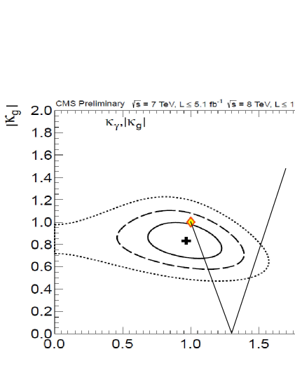
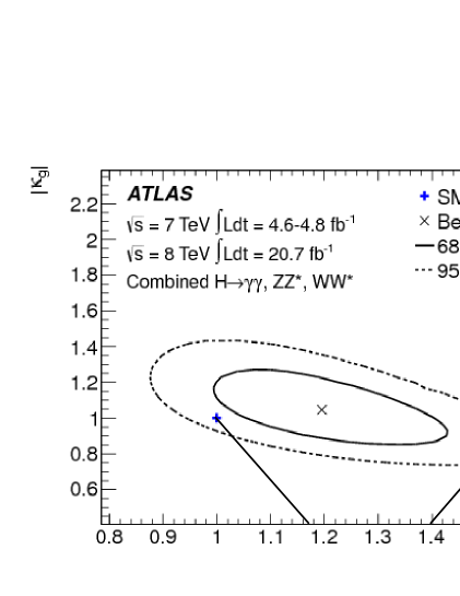
Fig. 3: CMS ( 68%, 95% and 99.7% CL) and ATLAS (68% and 95% CL) Collaboration likelihood contours for the scale factors $\kappa_{\gamma}$ and $\kappa_{g}$. The bent line represents the correlation between $\kappa_{\gamma}$ and $\mid\kappa_{g}\mid$ predicted by our model for positive values of the amplitude $K$.

Clearly the CMS and ATLAS results are consistent with our model at the 2 standard deviation level for small values of $K$ and $(\kappa_{\gamma},\kappa_{g})$ close to the usual SM values (1,1). We estimate upper limits for $K$ at the 3 standard deviation level in this case, corresponding to the first part of the bent line in Fig. 3 with $\kappa_{g}>0$, to be $K<K_{CMS}=0.24$ and $K<K_{ATLAS}=0.12$ for the CMS and ATLAS data respectively. However our model is also consistent with the ATLAS results at the 2 standard deviation level with values of $K\approx 0.8$ and $(\kappa_{\gamma}\approx 3/2,\kappa_{g}\approx-3/4)$, while only at the 3 standard deviation level with the CMS results.

In the following sections we estimate, as best we can, the value of the amplitude $K$ in our model by evaluating the loop diagrams in Fig. 2 for the bound states $S$ and $F$.

6 Form factor corrections

Our intuition suggests that the bound states $S$ and $F$ can in first approximation be treated as “fundamental” particles in loop calculations, due to the fact that they are so tightly bound. For this reason we introduce additional Feynman rules with propagators for the bound states and some appropriate coupling vertices. In principle, it should not be needed to do so, since at a very high order the long series of Feynman diagrams should produce the effects of bound states, but in practice we can hope to get meaningful and correct contributions using the propagators and vertices for the bound states. However the bound states are not really small compared to their Compton wavelengths in the Bohr hydrogen atom like model we use in appendix B to estimate the polarizability of $S$. Thus we expect to need form factors modifying the vertices or the propagators to be used, when the 4-momenta become of the order of the inverse radius of the bound state. We therefore propose the following crude rule for taking the structure of the bound states into account in Feynman loop integrals: When considering a bound state $i$ with an extension or radius $r_{0}=\sqrt{<r_{i}^{2}>}$, we introduce a form factor behaving like

$$\mathfrak{F}\approx\exp(\frac{1}{6}<r_{i}^{2}>q^{2}),$$ (26)

where $q$ is the four momentum relevant for the propagator (or effective vertex) in question. After a Wick rotation the loop four momentum $q$ will be space-like, so that $q^{2}<0$ and the contribution of the Feynman diagram is numerically damped.

So, in order to improve our estimate of the digrammatic contribution of bound states running around a loop, we suppose that exponential form factors (26), one for each propagator, come in multiplying the integrand of the Feynman diagram. This means that we include in the $q$-loop integral an extra factor

$${\mathfrak{F}}_{loop}=\exp(\frac{1}{6}<r^{2}>q^{2}),$$ (27)

where $<r^{2}>=\sum_{i}<r_{i}^{2}>$ is a quadratic sum of the radii of the particles, denoted by $i$, occurring around the loop.

We estimate the radii of our bound states using the Bohr model structure of appendix B. So we use the value

$$<r^{2}_{S}>=<r_{F}^{2}>=3a_{B}^{2}$$ (28)

for the spin-0 and spin-1/2 bound states $S$ and $F$, while for the spin-1 excited state $S_{1}^{*}$ we use

$$<r^{2}_{S_{1}^{*}}>=30a_{B}^{2}$$ (29)

for the 2p orbit. The Bohr radius $a_{B}$ is given by Eq. (43) of appendix B. Hence the squared radius parameter appropriate to the fermionic loop diagram of Fig. 2a for the bound state $F$ contribution is $<r^{2}>=3<r_{F}^{2}>=9a_{B}^{2}$. While in the bosonic loop diagram of Fig. 2b for the bound state $S$ contribution we have $<r^{2}>=2<r_{S}^{2}>+<r_{S_{1}^{*}}^{2}>=36a_{B}^{2}$.

7 Evaluation of bound state contributions

In order to compare our model predictions (24) for the scale factors $\kappa_{\gamma}$ and $\kappa_{g}$ with the CMS and ATLAS experimental data in Fig. 3, we need the value of the amplitude $K=-(12A_{S}+\frac{44}{3}\frac{m_{t}}{m_{F}}A_{F})$. So we now turn to the evaluation of the amplitudes $A_{S}$ and $A_{F}$.

Firstly we consider the amplitude $A_{S}$ introduced in Eq. (11) to parameterise the contribution of Fig. 2b to the Higgs diphoton decay. The dipole moment transition vertex $SS_{1}^{*}\gamma$ is defined in Eq. (52) of appendix B, where we introduce a scalar field $\phi_{S}$ for the bound state $S$ and an antisymmetric tensor field $V_{\mu\nu}$ for the spin-1 bound state $S_{1}^{*}$. The dipole moment tansition amplitude $d_{1}$ is estimated, in appendix B, using a calculation analogous to that of the dipole moment matrix elements for the hydrogen atom in atomic physics.

The mass $m_{S_{1}^{*}}$ of the excited bound state $S_{1}^{*}$ is expected to be much larger than the mass $m_{S}$ of the bound state $S$ and the Higgs mass $m_{H}$. So, in evaluating the amplitude for the loop diagram of Fig. 2b in appendix C, we actually take the large $m_{S_{1}^{*}}$ limit and integrate out the $S_{1}^{*}$ field. In this way, we effectively contract the propagator and the vertices involving the heavy bound state $S_{1}^{*}$ into a four-leg polarization vertex as illustrated in Fig. 4. The effective interaction corresponding to this four-leg polarization vertex is given in Eq. (51) of appendix B and the coupling constant is given by the polarizability $\alpha_{pol.}$ of the bound state $S$. The polarizability $\alpha_{pol.}$ is expressed in terms of the dipole moment transition amplitude $d_{1}$ in Eq. (44) of appendix B. Using the values of these parameters motivated by our atomic physics model of the bound states and a loop form factor ${\mathfrak{F}}_{0}(q^{2})=\exp(6a_{B}^{2}q^{2})$ from section 6, we evaluate the Feynman amplitude for Fig. 2b in appendix C. The following expression (75) is obtained:

$$-12A_{S}\approx\frac{2^{21}}{3^{13}}\frac{m_{t}^{2}}{m_{S}^{2}}=1.3\frac{m_{t}^{2}}{m_{S}^{2}}.$$ (30)

Fig. 4: The effective one loop diagram describing the contribution of $T_{s}$ – the scalar bound state S – to the diphoton decay of the Higgs boson.

The Feynman amplitude for the loop diagram of Fig. 2a for the spin-1/2 bound state $F$ is considered in appendix D. If $F$ were truly an elementary particle, the value of the amplitude $A_{F}$ in Eq. (11) would be given by $A_{1/2}(\tau_{F})\approx 1/3$. However this value is substantially reduced in the presence of the loop form factor ${\mathfrak{F}}_{1/2}(q^{2})=\exp(3a_{B}^{2}q^{2}/2)$ from section 6 for the bound state $F$. The resulting Feynman amplitude is estimated in appendix D, using the approximation that the mass $m_{F}$ of the 11 quark bound state $F$ is much larger than the Higgs mass $m_{H}$. The following expression (87) is obtained:

$$\frac{44}{3}A_{F}=0.034\left(\frac{m_{t}}{m_{F}}\right)^{3}.$$ (31)

The mass of the spin-1/2 bound state $F$ is expected to be much larger than that of the scalar bound state $S$ and the top quark mass. So we can neglect the contribution (31) of the bound state $F$ to the amplitude $K$ compared to the contribution (30) of the bound state $S$: $-12A_{S}\gg\frac{44}{3}\frac{m_{t}}{m_{F}}A_{F}$. Therefore we finally end up with the following expression for the amplitude $K$:

$$K=-12A_{S}\approx 1.3\frac{m_{t}^{2}}{m_{S}^{2}}.$$ (32)

8 Results

Our most secure result is the predicted correlation (24) between the scale factors $\kappa_{\gamma}$ and $\kappa_{g}$. Using our atomic physics based model for the four-leg polarization vertex and form factor corrections, we have evaluated the loop diagram of Fig. 4 to obtain our estimate (32) for the amplitude $K$ and hence for the scale factors:

$$\kappa_{\gamma}=1+0.80\left(\frac{m_{t}}{m_{S}}\right)^{2},\qquad\kappa_{g}=1-2.8\left(\frac{m_{t}}{m_{S}}\right)^{2}.$$ (33)

From the CMS and ATLAS data in Fig. 3, we estimated in section 5 the corresponding 3 standard deviation upper limits on the amplitude $K$ (for positive values of $\kappa_{g}$) to be $K_{CMS}=0.24$ and $K_{ATLAS}=0.12$ respectively. These limits lead, using Eq. (32), to the following estimates of the 3 standard deviation lower limits on the mass of our bound state $S$:

$$\mbox{CMS}\ 3\sigma\ \mbox{limit}:\quad m_{S}>400\ \mbox{GeV},\qquad\mbox{ATLAS}\ 3\sigma\ \mbox{limit}:\quad m_{S}>570\ \mbox{GeV}.$$ (34)

There is also a region of parameter space with negative values of $\kappa_{g}$ and $K\approx 0.8$, lying on the second part of the bent line in Fig. 3, which is consistent with the CMS and ATLAS data at better than 3 standard deviations. In fact the corresponding values of the scale factors

$$\kappa_{\gamma}\approx 1.5,\qquad\qquad\kappa_{g}\approx-0.75$$ (35)

are consistent with the CMS data at the $2.5\sigma$ level and with the ATLAS data at the $1.5\sigma$ level. We note that the latter fit to the ATLAS data is as good as the usual SM fit ($\kappa_{\gamma}$ = 1, $\kappa_{g}$ =1). From Eq. (32), we estimate the mass of the bound state $S$ giving rise to the scale factors (35) in our model to be:

$$m_{S}\approx 220\ \mbox{GeV}.$$ (36)

9 Conclusion

In this paper we have investigated further the proposed existence of a $6t+6\bar{t}$ scalar bound state $S$ and a $6t+5\bar{t}$ spin-1/2 bound state $F$, which are so strongly bound and exceptionally light that they effectively act as elementary particles to first approximation. We have estimated the loop corrections arising therefrom and the consequent scaling of the usual SM amplitudes for Higgs diphoton decay and for Higgs production via gluon fusion. Our predictions are rather uncertain due to the approximations we make and, in particular, to the large uncertainty on the mass $m_{S}$ of the bound state $S$.

We have compared our results for the scale factors $\kappa_{\gamma}$ and $\kappa_{g}$ with the LHC data of Fig. 3. We find two regions of allowable parameter space. They correspond to masses $m_{S}>400$ GeV for CMS or $m_{S}>570$ GeV for ATLAS data and $m_{S}\sim 220$ GeV respectively.

Our most robust prediction follows from the constituents of the bound states $S$ and $F$ being just top and anti-top quarks. Consequently there is a linear relationship between $\kappa_{\gamma}$ and $\kappa_{g}$, resulting from the effective proportionality between the relevant diagrams of Fig. 2 coupling the Higgs to two photons and the corresponding diagrams coupling it to two gluons. This relationship is represented by the bent line in Fig. 3 and is parameterised by the amplitude $K$ in Eq. 24. The diphoton decay width is expressed in terms of the amplitude $K$ and the usual SM contributions from $W^{\pm}$ and top quark loops as follows:

$$\Gamma(H\to\gamma\gamma)=\frac{\alpha^{2}m_{H}^{3}}{16\pi^{3}v^{2}}|A_{W}(\tau_{W})+\frac{4}{3}A_{t}(\tau_{t})-K|^{2}.$$ (37)

An analogous expression for the gluon fusion production cross section $\sigma(gg\to H)$ leads to Eq. 22.

The dominant contribution to the amplitude $K$ is provided by the loop diagram of Fig. 2b involving the color singlet self-conjugate 1s bound state $S$ of 6 top and 6 anti-top quarks. We treat its interaction with photons, or quite analogously with gluons, as due to the polarizability of the state $S$ by its being virtually excited up to a spin-1 state $S_{1}^{*}$ in which one of the quarks is excited to a 2p level. We estimate the polarizability $\alpha_{pol.}$ using a non-relativistic Bohr model and then translate it into a relativistic interaction using the procedure described in appendix A. The structure of the bound states is taken into account by form factors determined by their Bohr radii. The contribution of the spin-1/2 bound state $F$ turns out to give a relatively small contribution to $K$ and can be neglected.

The contribution of the loop diagram of Fig. 2b to the amplitude $K$ is estimated to be

$$K=\frac{9\alpha_{pol.}m_{t}m_{S}^{2}}{\pi\alpha}\int_{0}^{\infty}\mathfrak{F}_{0}(q_{E}^{2})\frac{q_{E}^{2}dq_{E}^{2}}{(q_{E}^{2}+m_{S}^{2})^{2}}\approx 1.3\frac{m_{t}^{2}}{m_{S}^{2}},$$ (38)

where $\mathfrak{F}_{0}(q_{E}^{2})$ is the form factor, discussed in section 6, for the $S$ bound state contribution. The bound state $S$ is supposed to be much lighter than $12m_{t}\sim 2$ TeV, but its mass $m_{S}$ is otherwise very uncertain. Realistically we would say our model requires $m_{S}<6m_{t}$ and hence $K>0.036$. This means that the deviations from unity of the scale factors $\kappa_{\gamma}$ and $\kappa_{g}$ should be greater than $2.2\%$ and $7.9\%$ respectively; otherwise our model is falsified. In a recent paper [16] we made a crude estimate of $m_{S}\approx 260$ GeV for the mass, which happens to be close to the mass of 220 GeV corresponding to the allowed region of parameter space with negative $\kappa_{g}$.

We emphasize again that this paper concerns the pure Standard Model. Usually one thinks that, apart from the strongly interacting gluons, the Feynman diagram expansion converges rather quickly. However if there are bound states, then in certain small regions it could be that the diagrams add up and produce a pole where the bound state is close to being on-shell. It is the existence of such a bound state that we propose here and, strictly speaking, are making a speculative correction to the usual SM calculation rather than introducing new physics. We do, however, suggest that the SM coupling constants are fine-tuned, by the so-called Multiple Point Principle, so as to produce a number of vacua with the same energy density. For this principle of degenerate vacua to be realized a bound state $S$ of 6 top and 6 anti-top quarks is needed to be exceptionally light. An analysis [9] of the complicated dynamics involved in the strong binding of the 12 quark state supports this conclusion, but the result has been disputed [38, 39, 40, 41] and more accurate but difficult calculations are needed.

Also it would be desirable to improve our Bohr model calculation of the polarizability of the bound state $S$ and of the form factors, by introducing the extra binding effects due to the exchanges of gluons, $W$’s etc and the other corrections discussed in Ref. [9]. It must though be admitted that this would mainly help fixing the value of the radius of the bound state, which we have seen may only influence our predictions mildly.

10 Acknowledgments

H.B. Nielsen thanks the Niels Bohr Institute for emeritus status and the University of Helsinki for a visit. L.V. Laperashvili deeply thanks the Niels Bohr Institute (Copenhagen, Denmark) for hospitality and financial support, and Roman Nevzorov (ITEP, Moscow) for very useful discussions. C.R. Das greatly thanks Prof. Utpal Sarkar for financial support through J.C. Bose fellowship. C.D. Froggatt thanks Glasgow University and the Niels Bohr Institute for hospitality and support.

Appendix A. Non-relativistic formulation of vertices

In the present article we introduce a standard procedure to translate from a non-relativistic expression for vertices involving our $6t+6\bar{t}$ spin-0 and spin-1 bound states $S$ and $S_{1}^{*}$ into a relativistic expression. We make a relativistic ansatz for a vertex and adjust the coefficient so that it matches the non-relativistic one. The basic rule followed is to use the usual relativistic normalization for, say, a scalar field $\int(2E)\phi^{\dagger}\phi d^{3}x=1$, and make the approximation $2E\approx 2m$. For example when we consider the $HSS$ vertex, treating the two scalar bound states $S$ as non-relativistic resting objects while $H$ is the interacting Higgs field, we get an extra factor $(\sqrt{2m_{S}})^{2}$ into the expression for the relativistic coupling constant (15):

$$G_{HSS}=12\frac{g_{t}}{\sqrt{2}}\cdot 2m_{S}.$$ (39)

In appendix B we transform the non-relativistic polarization Hamiltonian (40) into a relativistic expression (51) for the four-leg polarization vertex appearing in Fig. 4. We introduce the square of a scalar quantum field $\phi_{S}$ describing the scalar bound state $S$ into the Hamiltonian density (48) together with just two factors of $\sqrt{2m_{S}}$ to provide the correct relativistic normalization. We also introduce a normalization factor $\sqrt{2m_{S_{1}^{*}}}$ for the antisymmetric tensor field $V_{\mu\nu}$ associated with the spin-1 bound state $S_{1}^{*}$.

Appendix B: On describing the polarizability

In this appendix we discuss the interaction of $\gamma$-quanta with the bound states $S$ and $S_{1}^{*}$ given by the diagram of Fig. 2b and the effective interaction obtained by integrating out $S_{1}^{*}$ and given by the diagram of Fig. 4. This effective interaction, estimated in the non-relativistic limit of the bound state $S$ being essentially at rest, is described by the following polarization term in the Hamiltonian:

$$H_{pol.}=-\frac{1}{2}\alpha_{pol.}\vec{E}^{2},$$ (40)

where the constant $\alpha_{pol.}$ is called the polarizability. A model of polarizability is given in Refs. [46, 47].

When a neutral bound state is placed in an electric field $\vec{E}$, the positively charged part of it gets pulled in the direction of the field, and the negative cloud gets pulled in the direction opposite to the field. This results in the centres of positive and negative charge no longer being in the same place, so the bound state obtains a small dipole moment $\vec{d}$. Experimentally, it is found that for small fields this dipole moment is approximately proportional to the applied field:

$$\vec{d}=\alpha_{pol.}\vec{E}.$$ (41)

Let us now consider the dipole moment transition amplitude $d_{1}=qR_{1}$ for the bound state $S$, where $q=+2/3|e|$ and $R_{1}$ is the radius of transition from $S$ to the $S^{*}_{1}$-particle, which is a $2p$ excited state of the spin-0 $6t+6\bar{t}$ bound state $S$. We make an estimate of the value of $d_{1}$ based on the atomic physics calculation of the dipole moment matrix elements of the hydrogen atom. According to the atomic physics terminology, we have:

$$R_{1}=<2,1,0|z|1,0,0>=\sqrt{2}\frac{2^{7}}{3^{5}}a_{B}\approx 0.744a_{B},$$ (42)

where $a_{B}$ is the radius of the Bohr Hydrogen-atom-like bound state $S$, in which we approximate the interaction of each top quark by a central $1/r$ potential (neglecting the Higgs mass) while only half of the other 11 particles are present in the “nucleus” [10]. The variable $z$ denotes the position coordinate in an axial coordinate system. Therefore we have:

$$a_{B}=\frac{4\pi}{\frac{11}{2}(g_{t}^{2}/2)m_{t}}\approx\frac{5.2}{m_{t}}.$$ (43)

for a running top quark Yukawa coupling $g_{t}\approx 0.935$.

In the philosophy that the excited state $S_{1}^{*}$ of the ground state $S$ is a 2p state with an excitation energy equal to 3/4 of the ground state binding energy $E_{Ry}$, we obtain [47] the contribution of each of the 12 quark constituents to the polarizability of $S$ to be:

$$\alpha_{pol.}=\frac{2d_{1}^{2}}{\Delta E}=2q^{2}\frac{|<1s|z|2p>|^{2}}{\Delta E}$$ (44)

with

$$\Delta E=\frac{3}{4}E_{Ry}.$$ (45)

Here we used Heaviside-Lorentz units instead of the Gaussian units of Ref. [47]. In our case we have:

$$E_{Ry}=\frac{11g_{t}^{2}}{32\pi a_{B}}.$$ (46)

The value of the transition amplitude $<1s|z|2p>$ is given by (42), and Eq. (44) leads to the following result for the polarizability:

$$\alpha_{pol.}=4\pi\frac{e^{2}}{11g_{t}^{2}}\frac{2^{23}}{3^{13}}a_{B}^{3}.$$ (47)

The polarization Hamiltonian (40) is not relativistically invariantly as written and one should also note that there is no analogous magnetic interaction in the rest system of the bound state. So firstly we rewrite (40) as a Hamiltonian density in a quantum field theory like form, with a relativistically normalized self-conjugate scalar field $\phi_{S}$ describing the scalar bound state $S$ as explained in appendix A:

$${\cal H}_{polarization}=-\frac{\alpha_{pol.}}{2}(2m_{S})|\phi_{S}|^{2}\frac{1}{2}\vec{E}^{2}.$$ (48)

Then we perform an averaging over all possible Lorentz transformations of a corresponding Lagrangian density term, so as to obtain a Lorentz invariant expression by the replacement:

$$\frac{1}{2}{\vec{E}}^{2}\to\frac{1}{2}({\vec{E}}^{2}-{\vec{B}}^{2})\to\frac{1}{4}F_{\mu\nu}(x)F^{\mu\nu}(x),$$ (49)

where

$$\vec{E}|_{i}=F^{0i},\qquad\vec{B}|_{i}=\frac{1}{2}\epsilon_{ijk}F^{jk}.$$ (50)

Thus finally we obtain a covariant expression for the polarization Lagrangian density:

$${\cal L}_{pol.}(x)=m_{S}\frac{\alpha_{pol.}}{4}F_{\mu\nu}(x)F^{\mu\nu}(x)|\phi_{S}(x)|^{2}.$$ (51)

which replaces the polarization Hamiltonian as given by (40) for a single bound state at rest and describes the four-leg polarization vertex in Fig. 4.

The vertex $SS^{*}_{1}\gamma$ in the diagram of Fig. 2b is described by the interaction of the type

$$\frac{1}{2}d_{1}\sqrt{(2m_{S})(2m_{S_{1}^{*}}})\phi_{S}F^{\gamma}_{\mu\nu}V^{\mu\nu},$$ (52)

where $V_{\mu\nu}=-V_{\nu\mu}$ is an antisymmetric tensor field describing the vector particle $S^{*}_{1}$ and we have introduced the normalization factor $\sqrt{(2m_{S})(2m_{S_{1}^{*}}})$. In Eq. (52), an extra factor of 1/2 compensates for the fact that there is a double counting by the summation over the anti-symmetrized indices (here $\mu,\nu$). The effective field, called $V_{\mu\nu}$, which describes the excited bound state $S_{1}^{*}$, is only thought to be very crudely treated, and we thus only write here the main kinetic and mass terms for this field:

$${\cal L}(x)=\frac{1}{4}\partial_{\rho}V_{\mu\nu}\partial^{\rho}V^{\mu\nu}-\frac{1}{4}m_{S_{1}^{*}}^{2}V_{\mu\nu}V^{\mu\nu}-d_{1}\sqrt{m_{S}m_{S_{1}^{*}}}\phi_{S}F^{\gamma}_{\mu\nu}V^{\mu\nu}.$$ (53)

We do not go into detail with the terms destined to leave only the components of polarization properly oriented with respect to the four momentum of the $S_{1}^{*}$-particle – terms which contribute to the terms proportional to the momentum in the propagator (see (56) and (59) below), which we shall ignore in Appendix C.

Appendix C: Evaluation of the loop amplitude $\bf A_{S}$

The diphoton decay rate for the Higgs is given, in terms of the conventionally normalized Feynman integrals $I_{W,t,F,S}$ corresponding to the Feynman diagrams of Fig. 2, by

$$\Gamma(H\to\gamma\gamma)=\frac{1}{32\pi m_{H}}|I_{W}+I_{t}+I_{F}+I_{S}|^{2}.$$ (54)

A symmetry factor of 1/2 has been included in the phase space for the two identical photons and there is an implicit sum over their polarizations.

The usual SM expressions for $I_{W}$ and $I_{t}$ can be extracted from Section 3. We estimate $I_{F}$ in appendix D and find that it can be ignored compared to the other contributions $I_{W,t,S}$.

The last term from (54), which comes from the diagram of Fig. 2b, is more cumbersome. Indeed we shall take the limit of a very heavy spin-1 bound state $S_{1}^{*}$ and effectively integrate it out. We thereby replace the part of the diagram around the $S_{1}^{*}$-propagator by a single four-vertex, representing the polarizability of the bound state $S$ by virtual excitation to the $S_{1}^{*}$ state. Then we effectively have a diagram with just two vertices that appears when the $S_{1}^{*}$-propagator and the vertices attached at each end are contracted into one vertex with two incoming scalars $S$ and two outgoing photons. The corresponding diagram is given in Fig. 4.

Let us now estimate the Feynman integral $I_{S}$ for the loop diagram of Fig. 2b, using the vertex (52) from appendix B and the coupling $G_{HSS}$ of the Higgs field to the self-conjugate scalar bound state $S$. Taking into account that we have 12 different states of the top quark in the bound state $S^{*}_{1}$ (top quark and anti-top quark with 3 colors and 2 spin states), each of which can be excited into the 2p level, we obtain the following integral:

$$I_{S}=-i12G_{HSS}d_{1}^{2}m_{S}m_{S_{1}^{*}}\int\frac{d^{4}q}{{(2\pi)}^{4}}{\mathfrak{F}}_{0}(q^{2})\frac{1}{(q+k_{1})^{2}-m_{S}^{2}}\cdot\frac{1}{(q-k_{2})^{2}-m_{S}^{2}}\times$$

$$\frac{\Pi_{\mu\nu\mu^{\prime}\nu^{\prime}}}{q^{2}-m^{2}_{S^{*}_{1}}}\times[k_{1\mu}\epsilon_{\nu}(k_{1})-k_{1\nu}\epsilon_{\mu}(k_{1})][k_{2\mu^{\prime}}\epsilon_{\nu^{\prime}}(k_{2})-k_{2\nu^{\prime}}\epsilon_{\mu^{\prime}}(k_{2})].$$ (55)

Here

$$\Pi_{\mu\nu\mu^{\prime}\nu^{\prime}}=g_{\mu\mu^{\prime}}g_{\nu\nu^{\prime}}-\frac{q_{\mu}q_{\mu^{\prime}}}{m_{S^{*}_{1}}^{2}}g_{\nu\nu^{\prime}}-\frac{q_{\nu}q_{\nu^{\prime}}}{m_{S^{*}_{1}}^{2}}g_{\mu\mu^{\prime}}+\frac{q_{\mu}q_{\mu^{\prime}}q_{\nu}q_{\nu^{\prime}}}{m_{S^{*}_{1}}^{4}}.$$ (56)

and ${\mathfrak{F}}_{0}(q^{2})$ is the form factor (27) for the bound states propagating round the loop as estimated in section 6:

$${\mathfrak{F}}_{0}(q^{2})=\exp(\frac{1}{6}<r^{2}>q^{2}),$$ (57)

where

$$<r^{2}>=2<r_{S}^{2}>+<r_{S_{1}^{*}}^{2}>=36a_{B}^{2}.$$ (58)

We now assume the bound state $S_{1}^{*}$ is very heavy: $m_{S^{*}_{1}}\gg m_{S},\,m_{H}/2$, so we can replace the propagator of the bound state $S_{1}^{*}$ using the approximation:

$$\frac{\Pi_{\mu\nu\mu^{\prime}\nu^{\prime}}}{q^{2}-m^{2}_{S^{*}_{1}}}\approx-\frac{g_{\mu\mu^{\prime}}g_{\nu\nu^{\prime}}}{m^{2}_{S^{*}_{1}}}.$$ (59)

If we further make the identification

$$\Delta E=m_{S_{1}^{*}}-m_{S}\approx m_{S_{1}^{*}}$$ (60)

in the expression (44) for the polarizability, we obtain the following result:

$$d_{1}^{2}=\frac{1}{2}\alpha_{pol.}m_{S^{*}_{1}}.$$ (61)

Then, using the approximation (59) and the relations (61) and (15), we obtain:

$$I_{S}=i\frac{144\alpha_{pol.}}{v}m_{t}m_{S}^{2}\int\frac{d^{4}q}{{(2\pi)}^{4}}{\mathfrak{F}}_{0}(q^{2})\frac{1}{(q+k_{1})^{2}-m_{S}^{2}}\cdot\frac{1}{(q-k_{2})^{2}-m_{S}^{2}}\times$$

$$[(2k_{1}\cdot k_{2})(\epsilon_{1}\cdot\epsilon_{2})-2(k_{1}\cdot\epsilon_{2})(k_{2}\cdot\epsilon_{1})].$$ (62)

We note that we get the same expression for $I_{S}$ from Fig. 4, using the effective interaction (51) supplemented with the form factor ${\mathfrak{F}}_{0}(q^{2})$. This provides a useful consistency check on our calculation and also explains why the mass $m_{S_{1}^{*}}$ cancels out from our expression (62) for $I_{S}$.

We now make the approximation of neglecting the photon momenta $k_{1,2}$ as small compared to $m_{S}$ in the propagators of the expression (62) and obtain:

$$I_{S}=i\frac{144\alpha_{pol.}}{v}m_{t}m_{S}^{2}\int\frac{d^{4}q}{{(2\pi)}^{4}}{\mathfrak{F}}_{0}(q^{2})\frac{1}{(q^{2}-m_{S}^{2})^{2}}[(2k_{1}\cdot k_{2})(\epsilon_{1}\cdot\epsilon_{2})-2(k_{1}\cdot\epsilon_{2})(k_{2}\cdot\epsilon_{1})].$$ (63)

After the Wick rotation $q^{0}=iq_{E}^{4}$, $q^{2}=-q_{E}^{2}$ we have:

$$I_{S}=-\frac{144\alpha_{pol.}}{v}m_{t}m_{S}^{2}\int\frac{d^{4}q_{E}}{{(2\pi)}^{4}}{\mathfrak{F}}_{0}(q_{E}^{2})\frac{1}{(q_{E}^{2}+m_{S}^{2})^{2}}[(2k_{1}\cdot k_{2})(\epsilon_{1}\cdot\epsilon_{2})-2(k_{1}\cdot\epsilon_{2})(k_{2}\cdot\epsilon_{1})].$$ (64)

The symbol $E$ occurring as an index in (64) means that we are now using a Euclidean metric.

Taking into account that

$$\frac{d^{4}q_{E}}{{(2\pi)}^{4}}=\frac{q_{E}^{2}dq_{E}^{2}}{16\pi^{2}},$$

we obtain:

$$I_{S}=-\frac{144\alpha_{pol.}}{v}m_{t}m_{S}^{2}\int\frac{q_{E}^{2}dq_{E}^{2}}{16\pi^{2}}{\mathfrak{F}}_{0}(q_{E}^{2})\frac{1}{(q_{E}^{2}+m_{S}^{2})^{2}}[(2k_{1}\cdot k_{2})(\epsilon_{1}\cdot\epsilon_{2})-2(k_{1}\cdot\epsilon_{2})(k_{2}\cdot\epsilon_{1})].$$ (65)

We can also choose the polarizations $\epsilon_{i}$ for the photons to be orthogonal to both photon momenta $k_{1}$ and $k_{2}$. From the kinematics it is easy to see that $2k_{1}\cdot k_{2}=m_{H}^{2}$ on shell, and so we have:

$$I_{S}=-\frac{m_{H}^{2}}{16\pi^{2}}(\epsilon_{1}\cdot\epsilon_{2})\frac{144\alpha_{pol.}}{v}m_{t}m_{S}^{2}\int_{0}^{\infty}{\mathfrak{F}}_{0}(q_{E}^{2})\frac{q_{E}^{2}dq_{E}^{2}}{(q_{E}^{2}+m_{S}^{2})^{2}}.$$ (66)

Using the notation:

$$A_{0}=\int\frac{{\mathfrak{F}}_{0}(q_{E}^{2})q_{E}^{2}dq_{E}^{2}}{(q_{E}^{2}+m_{S}^{2})^{2}}=\int_{0}^{\infty}\frac{{\mathfrak{F}}_{0}(y)ydy}{(y+1)^{2}}=\int_{0}^{\infty}\frac{e^{-y/y_{0}}ydy}{(y+1)^{2}},$$ (67)

where

$$y=\frac{q_{E}^{2}}{m_{S}^{2}},\quad y_{0}=\frac{6}{m_{S}^{2}<r^{2}>},\quad{\rm{and}}\quad{\mathfrak{F}}_{0}(y)=e^{-y/y_{0}},$$ (68)

we have:

$$I_{S}=-\frac{m_{H}^{2}}{16\pi^{2}}(\epsilon_{1}\cdot\epsilon_{2})\frac{144\alpha_{pol.}}{v}m_{t}m_{S}^{2}A_{0}.$$ (69)

Now, by comparison of Eqs. (16) and (54), we have

$$I_{S}=\frac{\sqrt{2}\alpha m_{H}^{2}}{\pi v}12A_{S}.$$ (70)

Also, when the expression (69) for $I_{S}$ is inserted into (54), summing over the four polarization possibilities for the diphoton final state gives $|\epsilon_{1}\cdot\epsilon_{2}|^{2}=2$. So we can rewrite (70) in the form

$$I_{S}=\frac{\alpha m_{H}^{2}}{\pi v}\epsilon_{1}\cdot\epsilon_{2}12A_{S}.$$ (71)

It then follows from (69) that

$$12A_{S}=-\frac{36\alpha_{pol.}}{4\pi\alpha}m_{t}m_{S}^{2}A_{0}.$$ (72)

The radius parameter appearing in the form factor ${\mathfrak{F}}_{0}(q^{2})$ is estimated in section 6 and given in Eq. (58) as $<r^{2}>=36a_{B}^{2}$. Since this radius $<r^{2}>$ is large, it follows that $y_{0}$ is small:

$$y_{0}=\frac{6}{m_{S}^{2}<r^{2}>}=\frac{1}{6a_{B}^{2}m_{S}^{2}}\approx\frac{1}{160}\left(\frac{m_{t}}{m_{S}}\right)^{2},$$ (73)

and we can use the following approximation for the integral (67):

$$A_{0}\approx y_{0}^{2}=\frac{1}{36a_{B}^{4}m_{S}^{4}}.$$ (74)

Expressions for the Bohr radius $a_{B}$ and the polarizability $\alpha_{pol.}$ of the scalar bound state $S$ are given in terms of the top quark mass in (43) and (47) of appendix B. Substitution of these expressions into (72) and (74) gives:

$$-12A_{S}\approx\frac{4\pi}{11g_{t}^{2}}\frac{2^{23}}{3^{13}}\frac{m_{t}}{a_{B}m_{S}^{2}}=\frac{2^{21}}{3^{13}}\frac{m_{t}^{2}}{m_{S}^{2}}=1.3\frac{m_{t}^{2}}{m_{S}^{2}}.$$ (75)

Appendix D: Evaluation of the loop amplitude $\bf A_{F}$

In this appendix we estimate the Feynman integral $I_{F}$, appearing in (54), for the loop diagram of Fig. 2a for the spin-1/2 bound state F, using the coupling $G_{HF\bar{F}}$ of the Higgs field to $F$. Including a factor of 2 to incorporate the crossed diagram, we have:

$$I_{F}=C\int\frac{d^{4}q}{{(2\pi)}^{4}}{\mathfrak{F}}_{1/2}(q^{2})Tr\left[\frac{\not{q}+\not{k_{1}}+m_{F}}{(q+k_{1})^{2}-m_{F}^{2}}\gamma^{\mu}\frac{\not{q}+m_{F}}{q^{2}-m_{F}^{2}}\gamma^{\nu}\frac{\not{q}-\not{k_{2}}+m_{F}}{(q+k_{2})^{2}-m_{F}^{2}}\right]\epsilon_{\mu}(k_{1})\epsilon_{\nu}(k_{2}),$$ (76)

where the coefficient $C$ is

$$C=i2G_{HF\bar{F}}N_{c}Q_{t}^{2}e^{2}.$$ (77)

Here ${\mathfrak{F}}_{1/2}(q^{2})$ is the form factor (27) for the bound state $F$ propagating round the loop as estimated in section 6:

$${\mathfrak{F}}_{1/2}(q^{2})=\exp(\frac{1}{6}<r^{2}>q^{2}),$$ (78)

where

$$<r^{2}>=3<r_{F}^{2}>=9a_{B}^{2}.$$ (79)

We now assume the bound state $F$ is very heavy: $m_{F}\gg\,m_{H}/2$, so we can approximate the propagator of the bound state $F$ by $-1/m_{F}$. For example

$$\frac{\not{q}+\not{k_{1}}+m_{F}}{(q+k_{1})^{2}-m_{F}^{2}}\approx-\frac{1}{m_{F}}.$$ (80)

Then using (14) we obtain

$$I_{F} \approx i\frac{22m_{t}}{v}N_{c}Q_{t}^{2}e^{2}\int\frac{d^{4}q}{{(2\pi)}^{4}}{\mathfrak{F}}_{1/2}(q^{2})\left(-\frac{1}{m_{F}}\right)^{3}Tr\left[\gamma^{\mu}\gamma^{\nu}\right]\epsilon_{\mu}(k_{1})\epsilon_{\nu}(k_{2})$$ (81)

$$= -i\frac{88m_{t}N_{c}Q_{t}^{2}e^{2}}{vm_{F}^{3}}\epsilon_{1}\cdot\epsilon_{2}\int\frac{d^{4}q}{{(2\pi)}^{4}}{\mathfrak{F}}_{1/2}(q^{2}).$$ (82)

After the Wick rotation $q^{0}=iq_{E}^{4}$, $q^{2}=-q_{E}^{2}$ we have:

$$I_{F} \approx \frac{88m_{t}N_{c}Q_{t}^{2}e^{2}}{vm_{F}^{3}}\epsilon_{1}\cdot\epsilon_{2}\int\frac{q_{E}^{2}dq_{E}^{2}}{16\pi^{2}}{\mathfrak{F}}_{1/2}(q^{2})$$ (83)

$$= \frac{88\alpha m_{t}}{3\pi vm_{F}^{3}}\epsilon_{1}\cdot\epsilon_{2}\int q_{E}^{2}\exp(-3a_{B}^{2}q_{E}^{2}/2)dq_{E}^{2}$$ (84)

$$= \frac{352\alpha m_{t}}{27\pi vm_{F}^{3}a_{B}^{4}}\epsilon_{1}\cdot\epsilon_{2}.$$ (85)

Now, analogously to (71), we derive the relationship between $I_{F}$ and $A_{F}$ using Eqs. (16) and (54):

$$I_{F}=\frac{\alpha m_{H}^{2}}{\pi v}\epsilon_{1}\cdot\epsilon_{2}\frac{44}{3}\frac{m_{t}}{m_{F}}A_{F}.$$ (86)

It then follows from (85) that

$$\frac{44}{3}\frac{m_{t}}{m_{F}}A_{F}\approx\frac{352m_{t}}{27m_{H}^{2}m_{F}^{3}a_{B}^{4}}=0.018\left(\frac{m_{t}}{m_{H}}\right)^{2}\left(\frac{m_{t}}{m_{F}}\right)^{3}=0.034\left(\frac{m_{t}}{m_{F}}\right)^{3}.$$ (87)

where we have used the expression (43) for $a_{B}$ from appendix B.

References

- [1] C.D. Froggatt and H.B. Nielsen, Surveys High Energy Phys. 18, 55-75 (2003) [arXiv: hep-ph/0308144].
- [2] C.D.Froggatt, H.B.Nielsen, in Proc. to the Euroconference on Symmetries Beyond the Standard Model, (DMFA, Zaloznistvo, 2003) pp. 73-89 [ArXiv: hep-ph/0312218].
- [3] C.D. Froggatt, H.B. Nielsen and L.V. Laperashvili, Int. J. Mod. Phys. A 20, 1268 (2005) [arXiv: hep-ph/0406110].
- [4] C.D. Froggatt, L.V. Laperashvili and H.B. Nielsen, Phys. Atom. Nucl. 69, 67 (2006) [Yad. Fiz. 69, 3 (2006)]; [arXiv: hep-ph/0407102].
- [5] C.D. Froggatt, L.V. Laperashvili and H.B. Nielsen, in: Proceedings of 13th International Seminar on High-Energy Physics: QUARKS-2004, arXiv: hep-ph/0410243.
- [6] C.D. Froggatt, PASCOS 2004 Particles, Strings and Cosmology, edited by G. Alverson, E. Barberis, P. Nath and M.T. Vaughn (World Scientific, Singapore, 2005) pp. 325-334 [arXiv: hep-ph/0412337].
- [7] C.D. Froggatt, L.V. Laperashvili, R.B. Nevzorov, H.B. Nielsen and C.R. Das, Report CHEP-PKU-1-04-2008, CERN-PH-/2008-051TH, arXiv:0804.4506.
- [8] C.D. Froggatt and H.B. Nielsen, in Proceedings of the 34th International Conference on High Energy Physics (ICHEP08), Philadelphia, 2008, eConf C080730, [arXiv:0810.0475].
- [9] C.D. Froggatt and H.B. Nielsen, Phys. Rev. D 80, 034033 (2009) [arXiv:0811.2089].
- [10] C.R. Das, C.D. Froggatt, L.V. Laperashvili and H.B. Nielsen, Int. J. Mod. Phys. A 26, 2503 (2011) [arXiv:0812.0828].
- [11] C.R. Das, C.D. Froggatt, L.V. Laperashvili and H.B. Nielsen, in Proceedings of the 14th Lomonosov Conference on Elementary Particle Physics, edited by Alexander I. Studenikin (World Scientific, Singapore, 2010) pp. 379-381 [arXiv:0908.4514].
- [12] C.D. Froggatt, C.R. Das, L.V. Laperashvili and H.B. Nielsen, Yad. Fiz., 76, 172 (2013) [arXiv:1212.2168].
- [13] CMS Collaboration, CERN report CMS-PAS-HIG-13-005.
- [14] ATLAS Collaboration, ATLAS-CONF-2013-079.
- [15] ATLAS Collaboration (Georges Aad et al.), Phys. Lett. B 726, 88 (2013) [arXiv:1307.1427].
- [16] C. D. Froggatt and H. B. Nielsen, arXiv:1403.7177.
- [17] D.L. Bennett, H.B. Nielsen, Int. J. Mod. Phys. A 9, 5155 (1994).
- [18] D.L. Bennett, C.D. Froggatt, H.B. Nielsen, Report NBI-HE-94-44, in Proceedings of the 27th International Conference on High Energy Physics, Glasgow, 1994, edited by P.Bussey and I.Knowles (IOP Publishing Ltd, 1995) pp. 557-559.
- [19] D.L. Bennett, C.D. Froggatt, H.B. Nielsen, Perspectives in Particle Physics ’94, edited by D.Klabucar, I.Picek and D.Tadic (World Scientific, Singapore 1995) pp. 255-279 [arXiv: hep-ph/9504294].
- [20] C.D. Froggatt and H.B. Nielsen, Talk at 5th Hellenic School and Workshop on Elementary Particles, Corfu, 1995, Conference C95-09-03.1 [arXiv: hep-ph/9607375].
- [21] D.L. Bennett, C.D. Froggatt, H.B. Nielsen, in Proceedings of Seoul 1997, Recent developments in nonperturbative quantum field theory, Conference C97-05-26, pp. 362-393 [arXiv: hep-ph/9710407].
- [22] D.L. Bennett, H.B. Nielsen, in Proc. to the Euroconference on Symmetries Beyond the Standard Model, (DMFA, Zaloznistvo, 2003) pp. 235-246 [arXiv: hep-ph/0312218].
- [23] H.B. Nielsen and M. Ninomiya, arXiv: hep-th/0701018.
- [24] D.L. Bennett, in Proceedings to the 12th Workshop on ’What Comes Beyond the Standard Models? Bled, 2009 (DMFA, Zaloznistvo, Ljubljana, 2009) [arXiv:0912.4532].
- [25] C. D. Froggatt, H. B. Nielsen, Phys. Lett. B 368, 96 (1996) [arXiv: hep-ph/9511371].
- [26] N. Cabbibo, L. Maiani, G. Parisiand R. Petronzio, Nucl. Phys. B 158 (1979) 295.
- [27] P. Q. Hung, Phys. Rev. Lett. 42 (1979) 873.
- [28] M. Lindner, Z. Phys. C 31 (1986) 295.
- [29] M. Sher, Phys. Lett. B 317 (1993) 159: Addendum Phys. Lett. B 331 (1994) 448.
- [30] G. Altarelli and G. Isidori, Phys. Lett. B 337 (1994) 141.
- [31] J. A. Casas, J. R. Espinosa and M. Quiros Phys. Lett. B 342 (1995) 171.
- [32] J. Elias-Miro, J. R. Espinosa, G. F. Giudice, G. Isidori, A. Riotto and A. Strumia, Phys. Lett. B709 (2012) 222 [arXiv:1112.3022].
- [33] F. Bezrukov, M. Y. Kalmykov, B. A. Kniehl and M. Shaposhnikov, JHEP 1210 (2012) 140 [arXiv:1205.2893].
- [34] G. Degrassi, S. Di Vita, J. Elias-Miro, J.R. Espinosa, G.F. Giudice, G. Isidori, A. Strumia, JHEP 1208, 098 (2012) [arXiv:1205.6497].
- [35] D. Buttazzo, G. Degrassi, P. P. Giardino, G. F. Giudice, F. Sala, A. Salvio and A. Strumia, JHEP 12 (2013) 089 [arXiv:1307.3536].
- [36] C. D. Froggatt and H. B. Nielsen, Phys. Rev. Lett. 95 (2005) 231301 [arXiv: astro-ph/0508513]
- [37] C. D. Froggatt and H. B. Nielsen, Proceedings of the 8th Workshop on What comes beyond the Standard Model, Bled 2005 (DMFA, Zaloznistvo, Ljubljana, 2005) pp. 32-39 [arXiv:astro-ph/051245].
- [38] M.Yu. Kuchiev, Phys. Rev. D 82, 127701 (2010) [arXiv:1009.2012].
- [39] M.Yu. Kuchiev, V.V. Flambaum and E. Shuryak, Phys. Rev. D 78, 077502 (2008); [arXiv:0808.3632].
- [40] M.Yu. Kuchiev, V.V. Flambaum and E. Shuryak, Phys. Lett. B 693, 485 (2010) [arXiv:0811.1387].
- [41] Jean-Marc Richard, Few Body Syst. 45, 65 (2009) [arXiv:0811.2711].
- [42] J.R. Ellis, M.K. Gaillard and D.V. Nanopoulos, Nucl. Phys. B 106, 292 (1976).
- [43] M.A. Shifman, A.I. Vainshtein, M.B. Voloshin and V.I. Zakharov, Sov. J. Nucl. Phys. 30, 28711 (1979) [Yad. Fiz. 30, 1368 (1979)].
- [44] J.F. Gunion, H.E. Haber, G. Kane and S. Dawson, The Higgs Hunter’s Guide, Frontiers in Physics 80, Addison-Wesley (1990).
- [45] A. Djouadi, Phys. Rept. 457, 1 (2008) [arXiv: hep-ph/0503172].
-
[46]
D. Griffiths, Introduction to Electrodynamics, 3rd Edition,
Prentice Hall (2007),
Section 4.1.2, Problem 4.1. - [47] Gerald D. Mahan, Quantum Mechanics in a Nutshell, Princeton Press, N.Y., 2009.