Understanding pulsar magnetospheres with the SKA

Abstract:

The SKA will discover tens of thousands of pulsars and provide unprecedented data quality on these, as well as the currently known population, due to its unrivalled sensitivity. In this chapter, we outline the state of the art of our understanding of magnetospheric radio emission from pulsars and how we will use the SKA to solve the open problems in pulsar magnetospheric physics. Pulsars are known to be variable on numerous timescales: from nanoseconds to decades, corresponding to events, likely associated with the emission process itself through to discrete stable magnetospheric states. Timescales in between show phenomena such as pulse-to-pulse variations, sub-pulse drifting and nulling in operation, in addition to the relevant orbital, cooling and magnetic field decay timescales. The increased sensitivity and frequency range of the SKA will allow us to study these effects with higher fidelity than ever before. Moreover, it will be possible to perform these studies down to the individual pulse level for a large sample of millisecond pulsars. With their significantly different magnetic field strength and magnetospheric extent, this will provide important clues to the magnetospheric physics. Monitoring the SKA pulsar population, by fully exploiting its sub-arraying and multi-beaming capabilities, will enable us to study all of these phenomena and gain quantitative information on pulsar magnetospheres. Polarization profiles of a large number of pulsars, and their evolution over a broad frequency range, will enable us to perform measurements, with unprecedented detail, of the geometry of the emission regions of these systems. In addition to studying the plethora of new sources, we will perform intense targeted studies of already known objects. For example, with the SKA we will get a unique view of the magnetospheres of the two stars in the Double Pulsar System, down to the precision of a single rotation period, over a wide range of frequencies with full polarization information. We will be able to map the magnetospheres of selected sources by performing high sensitivity observations from 50 MHz all the way through to gamma-rays. Furthermore, using scintillation imaging techniques, we will be able to resolve pulsar magnetospheric features. With the good sample of radio-emitting magnetars, which the SKA pulsar surveys will provide, we will be able to compare, and identify any magnetospheric differences, between these and the standard pulsar population. As well as finally settling the questions about the pulsar emission mechanism and magnetospheric structure once and for all, we can use this understanding to improve the usefulness of pulsars as astrophysical tools. For example, understanding the switching behaviour in intermittent pulsars that is likely to be in operation in all pulsars at some level, and the detailed pulse-to-pulse modulation properties, will enable improved calibration of pulsar signals for use as precision clocks, which aides in the SKA’s headline science quests involving precision pulsar timing.

1 Pulsar magnetospheres and the SKA

Pulsar radio emission is used as a high precision tool in a number of astrophysical experiments. Currently, the most high profile experiments involve tests of gravity through pulsar timing, and the related search for a stochastic gravitational wave background. To take full advantage of the intrinsic rotational stability that characterizes pulsars, it is necessary to model all the effects that perturbe the measured pulse times-of-arrival. Over the past decade, the importance of modelling radio pulse propagation through the interstellar medium has been understood, and improvements are now becoming evident in timing residuals. This has revealed the next level of “timing noise”, most likely related to processes that occur near and within the radio emitting magnetosphere. For the first time, it is becoming clear that the lack of understanding of the pulsar radio emission mechanism is presenting obstacles to experiments that use pulsars as tools.

The quest to improve this situation with the SKA, relies on its ability to deliver the following elements:

1. high sensitivity, to observe individual pulses from pulsars at a high signal-to-noise ratio;
2. broadband receivers and backends, to study the frequency dependence of emission phenomena;
3. polarization, to better understand the pulsar geometries, the structure of the pulsar radio beams and the details of emission and propagation in the pulsar magnetosphere.
4. high-cadence monitoring, by observing multiple sources in sub-array mode, to uncover the physics that govern variability on all timescales.

The sole motivation to understand the radio emission mechanism is not to improve timing experiments. A steady stream of science output in areas such as relativistic plasmas in the magnetosphere, variability due to internal or external triggers, pulsar winds and supernova physics has resulted from the study of details of the radio emission mechanism on numerous interesting pulsars. The SKA surveys will deliver a new population of radio pulsars, among which we expect a group of sources that are ideal to address specific aspects of the emission mechanism problem (e.g. pulsars with interpulses for polarimetric studies of pulsar geometry).

In this chapter, we present the state of the art in observations aiming at understanding the magnetospheres of pulsars. We address this topic from three angles:

1. Understanding the three dimensional (3D) structure of the radio emission beam;
2.Understanding how magnetospheres evolve between different classes of pulsars;
3. Unlocking the information in the characteristic observational timescales of pulsar emission.

2 The radio emission beam

Our current understanding of the emission mechanism which operates in the magnetospheres of radio pulsars is limited. Progress can be achieved by determining where in the magnetosphere the radio emission is generated. Understanding where charged particles are accelerated to relativistic energies, would provide a better picture of the global pulsar electrodynamics, an essential element in solving the puzzle of how pulsars operate. In this section it is described how radio observations with the SKA are expected to advance our understanding of the elusive radio emission mechanism by allowing the construction of a 3D map of the pulsar magnetosphere.

2.1 Pulsar geometry and polarization

Radio polarization measurements allow geometrical properties of the radio beam to be quantified. Basic viewing geometry parameters include the magnetic inclination angle (angle between the magnetic dipole axis and the rotation axis of the neutron star) and the angle between our line-of-sight and the rotation axis. Since the early days of pulsar astronomy, the way the position angle of the linear polarization changes during the rotation of the star (PA-swing) is interpreted with the rotating vector model (Radhakrishnan & Cooke 1969; Komesaroff 1970, RVM), which directly depends on these two angles. Another important parameter of the emission beam, which can be derived using polarization measurements, is the radio emission height: co-rotation of the emitting region causes the PA-swing to be delayed with respect to the pulse profile, the magnitude of the shift being determined by the emission height (Blaskiewicz et al. 1991).

Currently, the viewing geometries have been derived for about a hundred objects (see e.g. Rankin 1990; Gould 1994), while emission heights are determined for only a fraction of those (e.g. Mitra & Rankin 2002; Rankin 1993; Weltevrede & Johnston 2008a). There are a number of complications which limit the precision and the fraction of the total population of pulsars suitable for this kind of analysis. Firstly, emission is only observed for a small interval of the rotation of the star. This limit makes a large range of RVM solutions become degenerate and in virtually all cases the viewing geometry cannot be determined from RVM fitting alone. In order to get unique solutions, additional assumptions are necessary. However, this introduces large and poorly understood systematics. Drawing statistical conclusions about the population as a whole is, therefore, known to be problematic, and emission heights determined in different ways often do not agree (see e.g. Mitra & Li 2004; Weltevrede & Johnston 2008a). Secondly, many pulsars do not have RVM-like PA-swings, showing that our understanding of pulsar polarization is incomplete. This severely limits the sample suitable for studying their viewing geometry. Moreover, because young pulsars are more suitable for this kind of analysis (see e.g. Johnston & Weisberg 2006; Weltevrede & Johnston 2008a) and references therein), the sample is necessarily biased. Thirdly, the above method to determine emission heights requires knowledge about which point in the radio profile corresponds to the closest approach of the line of light to the magnetic axis. Therefore knowledge about how the emission regions are distributed within the beam is crucial.

There is currently only one pulsar for which RVM fitting alone provide us with a unique viewing geometry without making additional assumptions (Kramer & Johnston 2008). This was possible because this pulsar has an interpulse (both magnetic poles are observed, which provides more rotational phase coverage) and it is young (therefore the PA-swing obeys the RVM very precisely). Simply observing currently known pulsars with a greater sensitivity is not expected to be effective, as systematic errors are the problem. The key is to find more of these “ideal case” pulsars, which then can be used to find out which additional assumptions are justified allowing emission geometries to be determined for a larger sample.

The SKA will discover many additional pulsars, including a sufficiently large “clean” sample of pulsars with RVM-like PA-swings to allow statistical studies of the pulsar population. As described above, this will be a biased sample in terms of their location in the $P$-$\dot{P}$ diagram. By comparing the results of the “clean” sample with the results of a larger sample the poorly understood biases can be investigated in detail. This ultimately will lead to a better understanding in the physical processes which are currently missing in models, thereby advancing our understanding of the emission mechanism.

As shown for instance by Dyks (2008), non-RVM-like PA-swings can teach us about the deformations of the magnetic field structure due to magnetospheric currents and rotational sweep-back of the magnetic field lines (see e.g. Dyks & Harding 2004). The determination of emission geometries can also be used to determine the way the magnetic inclination angle changes over time (Tauris & Manchester 1998; Weltevrede & Johnston 2008b; Young et al. 2010), which provides information about the torque acting on the pulsar. In addition, propagation effects of the radio waves in the pulsar magnetosphere are expected (e.g. Boyle & Pen 2012). Better understanding will allow the relevant plasma parameters of the emission mechanism to be determined. Good determination of emission geometry is also important for the study of drifting subpulses, as it allows the emission fluctuations observed for our line-of-sight to be related to a changing beam structure over time (see e.g. Deshpande & Rankin 2001; Vivekanand & Joshi 1997).

2.2 Radio emission regions

Despite the limited success at building a theoretical framework for the interpretation of pulsar radio emission, empirical models that attempt classifications of emission characteristics have uncovered observational patterns that any theory should be able to account for. For example, in a series of papers by Rankin and collaborators (Rankin 1983, 1990, 1993), evidence is presented that points to radio emission emanating from sets of active magnetic field lines, forming one, two or more hollow cones of emission. Different heights then correspond to different frequencies, in accordance with the observation that pulse profiles often become narrower towards high frequencies (e.g. Thorsett 1991). In addition to the hollow cones, Rankin’s classification included a type of component originating close to the magnetic axis which was labelled core. These often show distinguishing emission properties such as steeper spectra and complicated polarization features.

In contrast, Lyne & Manchester (1988) showed that the two-dimensional organization of radio components of a large population of pulsars is patchy, and although their characteristics broadly match the Rankin classification, there is no strong evidence of two emission mechanisms for core and cone emission. It was also noted that some young pulsars have observable emission from both magnetic poles. This property, coupled with the wide, relatively simple profiles of young pulsars and their polarization characteristics, was used by Johnston & Weisberg (2006) to suggest that radio emission originates from high altitudes in young pulsars compared to the older pulsar population. This idea was expanded further Karastergiou & Johnston (2007) to produce a phenomenological model that statistically explains the complexity of profiles from young and old pulsars (not millisecond pulsars). The main element of this model includes emission from a small number of discrete multiple heights for older pulsars, following ideas presented in Gangadhara & Gupta (2001). Multiple emission heights have implications on geometrical modeling.

Broadband observations, polarization and sensitive single pulse observations are all essential to understanding the detailed 3D location of radio emission regions in pulsar magnetospheres.

2.3 Radio spectra and broadband nature of emission

The radio emission of pulsars is produced by relativistic particles in the circumpulsar plasma. Pulsar spectra must be explained by a model which describes the emission mechanism, in combination with the energy distribution of the particles responsible for the observed emission (e.g. Malofeev & Malov 1980). Therefore, detailed measurements of pulsar spectra provide valuable information about how the radio emission is produced. In addition, understanding the pulsar spectrum in a statistical sense for the pulsar population is crucial for population synthesis to refine models for the parent distribution of pulsars, which gives rise to the observed distribution (Bates et al. 2013).

The spectra of radio pulsars are broadband and resemble (at least to first order) power laws with a relatively steep frequency dependence. Above $\sim$200 MHz the average spectral index was shown by Maron et al. (2000) to be $-1.8$, with a standard deviation of 0.2 (i.e. pulsars are brighter at lower frequencies), although Bates et al. (2013) suggest a mean spectral index closer to $-1.4$ with unity standard deviation. The dependence on pulsar parameters, such as $P$ and $\dot{P}$, is weak, but correlations with characteristic age are found (Lorimer et al. 1995). Understanding the way spectra depend on the spin parameters will give insight into how magnetospheric conditions change throughout the $P-\dot{P}$ diagram.

In general, deviations are observed from this first order behavior, one of which is that at lower frequencies, the spectrum often “turns over” (e.g. Sieber 2002, and references therein). It is currently unknown if this is because of a decrease in efficiency of the emission mechanism, or because of an absorption mechanism becoming effective. It is also not known why some pulsars do not have these low-frequency turnovers, but others do. There is a hint that these spectral turnovers do not happen for millisecond pulsars (Kuzmin & Losovsky 2001), suggesting that their magnetospheric conditions are significantly different compared to normal (non-recycled) pulsars. Apart from the lack of a spectral break at low frequencies the spectra of MSPs and slow pulsars are remarkably similar (Kramer et al. 1998). At higher frequencies ($\sim 10$ GHz or above) spectral breaks are observed, such that the spectrum flattens or even turns up (Wielebinski et al. 1993; Kramer et al. 1997).

A complication in the interpretation of radio spectra is that the observed spectrum is affected by a geometric feature. This feature arises because the beam shape is frequency dependent such that we see different parts of the beam at different frequencies. An understanding of this effect is therefore crucial to infer the intrinsic spectra from those observed.

2.4 The interstellar medium as an interferometer of resolved pulsar magnetospheres

Interstellar scintillation affords the potential to resolve the tiny emission regions of pulsars. By virtue of the compactness of the emission, pulsar radiation is subject to strong interference effects as it propagates through the turbulent plasma of the Interstellar Medium (ISM). However, pulsar magnetospheres have a finite size and, for extended sources, each ray path produces a subimage. The radiation observed at Earth is the result of the interference between many thousands of sub-images, or speckles, across the scattering region. Since the scale of the speckle pattern exceeds $\sim 10$ AU in some cases (e.g Brisken et al. 2010), interstellar scattering offers the prospect of achieving picoarcsecond angular resolution. Scintillation-based tests of the emission size fall into three broad categories according to the manner in which the finite size of the emission region manifests itself on the radiation properties.

An angular displacement in the emission site causes a lateral displacement in the scintillation pattern at Earth. If that displacement is parallel to the direction of motion of the pulsar, and the turbulence is “frozen”, then a lag in time produces precisely the same effect on the scintillation pattern as a change in pulse phase. This technique was applied by Wolszczan & Cordes (1987) during a double imaging event to place an upper limit on the emission size of PSR B1237+25 of $10^{6}$ km, roughly an order of magnitude larger than its light cylinder.

Although the different lines of sight from the source are coherent, the different parts of the subimages are not. For a point source, interference forms a diffraction pattern, a “scintillation pattern”, in the observer plane. The intensity varies randomly from zero to many times the average; indeed, zero intensity is the most common value. A resolved source forms a superposition of diffraction patterns from each individual point on the source; these points are not coherent, so that the observed pattern is the incoherent superposition of the patterns from a point source. The effect upon the diffraction pattern depends on the size of the source, with a typical scale of the angular resolution of the scattering region, viewed as a lens, as the size of a source that affects the distribution of intensity significantly. The observed distribution of intensity, or of interferometric visibility, provides a measure of the size of the source. Comparison of the pattern between two widely spaced observatories can provide information on the shape of the source. The technique was used by Gwinn et al. (2012) to measure a size for the emission region of the Vela pulsar of $<100$ km to $~{}1000$ km, with the smallest size near pulse center and the largest at the beginning and end. A single-dish technique was used by Johnson et al. (2012) to set an upper limit of $<40$ km, averaged over the entire pulse. The difference in measured size may reflect the emergence of an additional, “conal” component at the shorter wavelength, the broader pulse, or other factors.

The technique of speckle scintellometry extends the technique that deduces the emission region structure based on the lateral displacement of the scintillation pattern by using holographic techniques to further boost the S/N of the pulsar signal by partially descattering the radiation (Walker et al. 2008). Application of this technique to PSR B0834+06 yields a determination of the astrometric phase shift across the pulse profile equivalent to an angular resolution of 150 picoarcseconds, or 10 km at the distance of the pulsar (Pen et al. 2014).

2.5 Neutron Star Precession

2.5.1 Mapping pulsar beams

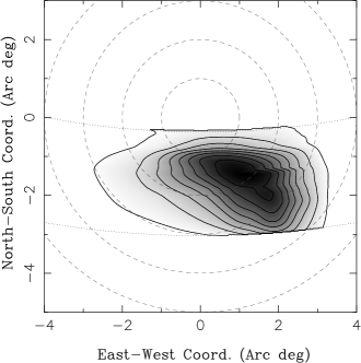
Figure 1: Two-dimensional shape of the emission beam over the traversed region in PSR J1141–6545. The inclination of the magnetic axis is taken to be $160^{\circ}$. The dotted lines show the path traversed by the line of sight; the lower one corresponds to the beginning of the data span and the upper one to the minimum impact parameter reached around MJD 54000. For more details see Manchester et al. (2010).

The observed pulse profiles show a large variety of shapes produced by a one-dimensional cut through the two-dimensional intensity distribution given by the pulsar beam. In General Relativity, the proper reference frame of a freely falling object suffers a precession with respect to a distant observer, called geodetic precession. In a binary pulsar system, this geodetic precession leads to a relativistic spin-orbit coupling, analogous to spin-orbit coupling in atomic physics. As a consequence, the pulsar spin axis precesses about the total angular momentum vector, changing the relative orientation of the pulsar towards Earth. In such a case, we should expect a change in the radio emission received from the pulsar, as first proposed by Damour & Ruffini (1974) very soon after the discovery of PSR B1913+16. Indeed, as our line-of-sight moves through the emission beam, each profile represents a slightly different cut through the beam structure. By adding measured profiles in the right order, it is possible to reconstruct a real 2-D map of a pulsar beam. One also expects that the polarization will change with time. Currently, such an experiment has been successfully applied to PSRs B1913+16 (Weisberg & Taylor 2002; Clifton & Weisberg 2008; Kramer 2002), J1141$-$6545 (Manchester et al. 2010) (see Fig. 1), J1906+0746 (Kasian 2012) and recently J0737$-$3039B (Perera et al. 2010). The results are so far inconclusive as to whether a systematic pattern exists.

2.5.2 Free precession

Free precession is the most general motion executed by a rotating solid body. Given that neutron stars have elastic crusts (and may contain solid components in their core, according to some nuclear physics models), they can sustain asymmetries which may lead to the system precessing. In order to illustrate the main issues, let us consider the case of PSR B1828–11, which provides the strongest evidence in favour of free precession so far (Stairs et al. 2000). Possible precession solutions for the data, which shows periodicity at both around 500d and 1000d, were first discussed in Jones & Anderson (2001); Link & Epstein (2001). More recently, it has been argued that the observed periodicity does not in fact represent free precession but is a result of state-switching in the magnetosphere (Lyne et al. 2010). However, as argued in Jones (2012), this does not necessarily mean that precession does not play a role in the system.

If we, for the moment, assume that PSR B1828–11 is freely precessing, then Jones & Anderson (2001) argue that the data requires the magnetic dipole to be very nearly orthogonal to the star’s deformation axis (associated with the asymmetry that forces the precession). This would lead to an inferred wobble angle in excellent agreement with the value estimated from the amplitude modulation. The data for PSR B1828–11 is at variance with the level of superfluid pinning required to explain the large glitches seen in the Vela pulsar. It also does not allow for the expected pinning of superfluid vortices to magnetic fluxtubes in the star’s superconducting core (Link 2003). At the moment we seem to have three options: i) Our understanding of neutron stars superfluidity/superconductivity is not quite right (Link 2003), ii) various instabilities may intervene and affect the fluid motion, thus altering the conclusions (Glampedakis et al. 2008), or iii) we are not seeing free precession (Lyne et al. 2010).

3 Energetics of pulsar magnetospheres and radio emission

Within the pulsar population, there are particular populations with clear and to some extent interpretable emission characteristics (Tauris et al. 2014). The SKA pulsar surveys will allow for new breakthroughs (Keane et al. 2014) by providing significantly more examples from each of the populations described in the following.

3.1 Young Pulsars

The youngest pulsars, which have the highest spin-down energy loss rates, appear to have different emission properties to the more middle-aged pulsars. In particular, they possess extremely high levels of linear polarization (Johnston & Weisberg 2006; Weltevrede & Johnston 2008a), not generally seen in the older pulsars. Furthermore, the polarization position angles follow the RVM curve to a much greater degree than the old pulsars do; this is particularly important in determining their geometry (see section 2.1). Curiously, it appears as if the orientation of their linear polarization is either parallel to the magnetic field or perpendicular to it (Johnston et al. 2005; Rankin 2007). This can be understood in terms of plasma physics, which predicts orthogonal polarization modes (Manchester et al. 1975). Some evidence suggests that the younger pulsars have ‘simpler’ profiles to those of the middle-aged pulsars (Karastergiou & Johnston 2007).

The majority of young pulsars are also high-energy emitters. Since the launch of the Fermi satellite more than 200 pulsars are now known to be $\gamma$-ray emitters (Abdo et al. 2013). The relationship between the $\gamma$-ray emission and the radio emission is a critical one to our understanding of the magnetosphere. Much progress has been made in this area in recent times, but results are still inconclusive (see e.g. Watters et al. 2009; Romani & Watters 2010; Pierbattista et al. 2012). This class of pulsars is likely to grow in importance as more high-energy pulsars are detected.

3.2 Magnetars

Magnetars are a class of neutron stars composed of Anomalous X-ray Pulsars (AXPs) and Soft Gamma-ray Repeaters (SGRs). Currently there are 21 magnetars detected with 5 more awaiting confirmation . Originally, SGRs were discovered to have bursting emission in the hard X-ray/soft gamma-ray range (Mazets et al. 1979), while AXPs are steady, X-ray emitting sources with rotational periods exceeding few seconds (Fahlman & Gregory 1981). Subsequent observations of powerful bursts from AXPs (Gavriil et al. 2002), as well as the discovery of persistent X-ray emission and slow rotational periods from SGRs (Kouveliotou et al. 1998) have revealed the common nature of their emission properties (Duncan & Thompson 1992). Magnetars were typically known to share the following properties: very strong magnetic fields exceeding the quantum critical value for electrons ($B\sim 4.4\times 10^{14}$ G); decay of such fields is believed to create the observable high X-ray and gamma-ray luminosities (Thompson & Duncan 1995, 1996), often visible in bursts; spin periods of 5 – 12 s with rapid spin-down on timescales of $10^{3}-10^{5}$ years; and absence of radio emission.

Recent discoveries of pulsars with spin periods and inferred dipolar magnetic field strengths typically seen in magnetars (Camilo et al. 2000; McLaughlin et al. 2003) and at which radio emission should not occur, bring magnetars and pulsars closer as a single population. The detection of transient radio emission from XTE J1810–197 and 1E 1547–5408 (Camilo et al. 2006, 2007a), followed by the discovery of PSR J1622–4950, a magnetar first detected in radio (Levin et al. 2010) with subsequent identification of its X-ray counterpart (Anderson et al. 2012), further strengthens this link. Another example is SGR J1745–2900, the only radio emitting magnetar found in the inner parsec of the Galactic Centre (Eatough et al. 2013; Shannon & Johnston 2013). The radio emission from magnetars is highly variable in nature and usually declines in tandem with its higher energy counterparts. Magnetar radio emission typically appears after X-ray outbursts; has a flat spectral index (Lazaridis et al. 2008) which enables detection even of individual pulses at frequencies above 88 GHz (Camilo et al. 2007d); shows pulse profile morphology changing dramatically on timescales of minutes to days (Camilo et al. 2007c, b; Levin et al. 2013); shows polarization similar to the emission properties of normal radio pulsars but with differences which can be explained as propagation effects in a non-dipolar magnetic field (Camilo et al. 2008; Kramer et al. 2007). Fig. 2 shows a typical observation of XTE J1810–197 with the 100-m Effelsberg radio telescope at 8.35 GHz.

The population of radio magnetars is very small at present. As they emit over a wide spectrum of wavelengths ($\gamma$-ray, X-ray, optical, near infrared and radio) studies at multiple frequencies are best poised to provide information on these objects. The SKA pulsar surveys will significantly increase the sample of radio emitting magnetars and uncover their relationships with the other populations of radio emitting neutron stars.

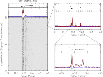
Figure 2: Left: Pulse stack from an 8.35 GHz observation with the average profile and position angle swing plotted on top. Total intensity is plotted in black, while linear and circular polarization are plotted in red and blue respectively. Top right: Individual single pulse profile with visible narrow and spiky emission. Bottom right: Close-up of the pulse plotted above.

3.3 Millisecond Pulsars

Most of our current knowledge of the pulsar emission mechanism and pulsar magnetospheres is derived from observations of slow pulsars. Only a very limited number of the known millisecond pulsars (MSPs) is bright enough to enable detailed studies of their single-pulse and magnetospheric properties. However, the studies that have been performed so far have shown interesting differences between MSPs and slow pulsars, motivating detailed studies of MSPs at the high sensitivity provided by the SKA.

The first clear difference between MSPs and slow pulsars is that the RVM cannot explain the polarimetry of MSP emission, even though other polarimetric properties (such as polarization degree and the presence of orthogonally polarized modes), do not differ (Yan et al. 2011). Similarly ambiguous results are found in the profile variations as a function of observing frequency: even though the pulse profiles of MSPs vary less strongly (which indicates a far smaller emission region than in the case of slow pulsars), the overall changes are reminiscent of slow pulsars, but shifted to higher frequencies (Kramer et al. 1999). Concerning intensity variations of single pulses, Jenet & Gil (2004) found no variations (other than giant pulses) in PSR B1937+21, while clear pulse-to-pulse modulations were found in PSR J0437-4715 (Jenet & Gil 2004; Osłowski et al. 2014). Edwards & Stappers (2003) discovered giant pulses in several pulsars and possible sub-pulse drifting. For the brightest MSP, PSR J0437-4715, the recent work by Osłowski et al. (2014) rules out drifting sub-pulses.

In summary, a clear picture of the emission properties of MSPs has yet to emerge. The lack in telescope sensitivity has limited this area of research to essentially the two brightest MSPs, which are far from representative of the whole MSP population in many regards. Early indications do show that the emission mechanism for slow pulsars and MSPs must be similar, if not identical. Understanding the emission process in MSPs is an essential element in the continued research of pulsar magnetospheres.

3.4 The double pulsar

The double pulsar PSR J0737$-$3039A/B is not only a remarkable system in the context of testing gravity theories; it also provides a unique window of opportunity to study pulsar magnetospheres. This binary comprises a rapidly spinning 23-ms pulsar, A, in a 2.4-hr orbit with a slowly rotating 2.8-s pulsar, B. The fortunate nearly edge-on alignment of the orbit with our sight line is such that pulsar A is eclipsed for $\sim 20$ s when it passes behind pulsar B. The duration implies a transverse cross-section of a few km at the location of pulsar B from A, thus implying a magnetospheric origin. A high time resolution study by McLaughlin et al. (2004) revealed that the eclipsed signal from A is modulated by the rotation of B during the eclipse, a phenomenon which led Lyutikov & Thompson (2005) to interpret the eclipses as being caused by synchrotron resonance in the closed field lines of pulsar B. The modulation naturally arises from the change in optical depth as the magnetic field geometry changes over the course of B’s rotation. Subsequently, Breton et al. (2008) demonstrated the success of this model in a long-term study of the radio eclipses, which led to the direct measurement of relativistic spin precession of pulsar B.

The double pulsar eclipses have two majors implication for the study of pulsar magnetospheres. Firstly, they allow us to directly probe the topology of a pulsar’s magnetic field, which has been shown to be primarily dipolar (Breton et al. 2012). Secondly, multi-frequency observations of the eclipse profile can constrain plasma properties such as the density, profile and multiplicity of the plasma. It has been shown that the density profile drops abruptly at a radius well inside the co-rotation radius (i.e. light cyclinder) and requires a large multiplicity (Breton et al. 2012). SKA1 will allow us to perform a polarization study of the eclipses which will yield an independent test of the eclipse mechanism and geometry of the system (Lyutikov & Thompson 2005). Polarization studies will also allow us to infer the strength of the magnetic field and compare it to predictions from pulsar timing.

4 Timescales in pulsar magnetospheres

While it has been known since the early days of pulsar astronomy that individual pulses are intrinsically variable, over the past decade a number of important observational results have shown that both radio emission and the magnetosphere itself can vary on timescales spanning at least $18$ orders of magnitude, from nanoseconds to decades. In the following, we describe the current understanding of radio emission phenomenology on all timescales and how this relates to pulsar timing experiments. It is important that SKA pulsar observation scheduling is determined by our understanding of the timescales of magnetospheric variability, in order to maximize scientific return.

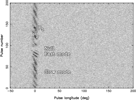
Figure 3: A pulse-stack of successive radio pulses of PSR B1819$-$22. The radio intensity (darker is brighter) is plotted as function of rotational phase (or longitude) versus pulse numbers. The emission (in the subpulses separated by $P_{2}$) appear to “march” in rotational phase from pulse to pulse creating a distinct pattern which repeats itself every $P_{3}$ pulses, a phenomenon called “drifting subpulses”. In addition this pulsar shows “mode changes”, which in this case manifests itself as two distinct drift modes: the slow and fast mode. The pulsar also has a “null” state, i.e. for a few stellar rotations there was no radio emission emitted by the pulsar. This figure shows 1380 MHz data obtained by the Westerbork Synthesis Radio Telescope (Weltevrede et al. 2006).

4.1 Short timescale phenomena

Radio pulsars display a myriad of amplitude modulation effects, as seen in Fig. 3. Averaged over many rotations, most pulsars have a reproducible pulse shape, reflective of the long-term stability of their rotation and magnetic fields. However, pulse shape and intensity can vary considerably in sequential rotations of a pulsar. Ordered and stochastic processes affect some pulsars to varying degrees; ordered modulations include sub-pulse drift (gradual phase shift of pulse peak), mode changing (regular changes between two or three distinct pulse shapes), and nulling (cessation of the radio beam). Pulse statistics using full polarimetry (Stinebring et al. 1984a, b; Karastergiou et al. 2002; Mitra et al. 2007) have led to gradual improvement of our understanding of orthogonal mode emission (McKinnon 2003; Edwards & Stappers 2004). Drifting sub-pulses in PSR B0943+10 led Deshpande & Rankin (2001) to champion the ‘rotating carousel’ model for the circulation of the pulsar beamlets (see e.g. Rankin et al. 2006; Mitra & Rankin 2008). However, it is far from clear if this model can be applied in every case of drifting subpulses and other models have been proposed (e.g. Clemens & Rosen 2004).

It is also of particular interest to understand contributions of pulse-to-pulse variability to precision pulsar timing, referred to as jitter noise. Correcting, or at least accounting for, jitter noise is imperative for optimizing strategies for SKA pulsar timing activities (Shannon et al. 2014). The brightest MSPs at decimetre wavelengths, PSR J0437$-$4715 and J1713+0747, have been the most extensively studied (Shannon & Cordes 2012; Osłowski et al. 2014). While the emission of these two millisecond pulsars show many similarities to that of slower pulsars, many of the classic single pulse phenomena, such as drifting subpulses or pulse nulling are not observed (Vivekanand et al. 1998).

Pulse nulling, where the radio emission appears to switch off, was one of the first phenomena identified (Backer 1970b), and is the prototypical example of pulsar variability (see review by Biggs 1992). In the “classical” nullers, emission is observed to switch off and on rapidly (few tens of pulses) and some pulsars had a relatively high “off” fraction (Wang et al. 2007). It came as a major surprise when McLaughlin et al. (2006) discovered pulsars, which only produce one pulse of emission every tens of minutes (the so-called RRATs). Several tens of these objects have now been found (McLaughlin et al. 2009). Because their duty cycle is so low, their population could rival that of the normal pulsars (Keane & Kramer 2008).

Kerr et al. (2014) show that several distinct timescales are present in the PSR J1717$-$4054, which has both long (many hours) and short (few seconds) nulling periods. The broadband nature of pulse nulling was investigated by Bhat et al. (2007). Our knowledge of how these various populations fit together is given by Burke-Spolaor et al. (2012).

Other effects such as intense giant pulses (Staelin & Reifenstein 1968; Comella et al. 1969) or “giant micropulses” (Johnston et al. 2001) occur in some pulsars at a limited phase range. The energy distribution of radio pulses can provide a window into the state of pulsar plasma and the method of emission generation. There exist a great number of viable plasma-state models, a few of which predict pulse energy distributions; the most commonly-proposed predictions are of Gaussian, log-normal, and power-law distributions. Cairns et al. (2001, 2003) and references therein, provide discussion on these models. Energy distributions have now been examined in detail for a number of pulsars (Burke-Spolaor et al. 2012), demonstrating that most pulsars obey log-normal statistics. These analyses have substantially contributed to the hypothesis that genuine “giant pulses” are generated separately from standard pulse generation and are much more rare. Giant pulses appear to have power-law energy distributions, distinct from the otherwise log-normal main pulse components (Lundgren et al. 1995; Johnston & Romani 2002).

It was giant pulses that led to the discovery of the Crab pulsar (Staelin & Reifenstein 1968). Classical Crab pulsar giant pulses are characterized by their appearance at the same phase range as the high-energy emission (Lundgren et al. 1995), high flux densities (Hankins et al. 2003; Popov & Stappers 2007), and power-law intensity distributions (Argyle & Gower 1972; Lundgren et al. 1995), Since the discovery of the Crab pulsar, other giant pulse emitters have been observed, both in young pulsars (like for instance the Crab twin PSR B0540-69 Johnston & Romani 2003), and in millisecond pulsars (Cognard et al. 1996; Romani & Johnston 2001; Knight et al. 2006). Common aspects between all giant pulse emitting pulsars are currently not known. Giant pulses in the Crab seem to share properties such as their short pulse widths down to 0.4 ns (Hankins et al. 2003; Hankins & Eilek 2007), and high brightness temperatures up to 10³⁹ K (Soglasnov et al. 2004), indicating coherent emission mechanisms. In addition to the giant pulses, bright, rare, ‘spiky’ emission is seen in other pulsars, for example the bursty emission in PSR B0656+14 (Weltevrede et al. 2006), the giant-like pulses from PSRs J1048–5832 and J1709–4429 (Johnston & Romani 2002) and the giant micro-pulses from the Vela pulsar (Johnston et al. 2001).

A number of tests of pulsar models can be performed using the statistics of per-rotation pulsar modulation. Weisberg et al. (1986) first noted differences in modulation between core and conal-type pulse profiles, while Jenet & Gil (2003) derived theoretical predictions for anti-correlations between pulse-to-pulse modulation and four “complexity parameters,” corresponding to four pulsar emission models. Their complexity parameters are: $a_{1}=5\dot{P}^{2/6}P^{-9/14}$, for the sparking gap model, $a_{2}=(\dot{P}/P^{3})^{0.5}$ for the continuous current outflow instabilities, $a_{3}=(P\dot{P})^{0.5}$ for surface magnetohydrodynamic wave instabilities, and $a_{4}=(\dot{P}/P^{5})^{0.5}$ for outer magnetospheric instabilities. Few observational studies have been done to test these effects, however the Jenet & Gil (2003) study for a small sample of core-type profiles disfavoured the magnetohydrodynamic wave instability model, and the study of $\sim$190 pulsars (Weltevrede et al. 2006, 2007) at 21 and 92 cm indicated that the modulation index is generally higher at lower frequencies, and noted a weak correlation between modulation index and age that is dampened at higher frequency.

The study of single-pulse modulation in a large pulsar sample can also contribute to several practical questions, for instance: how common is giant-pulse emission? Are the prospects of pulsar detection in other galaxies better for single-pulse or Fourier searches? Quantification of pulsars’ modulation will also aid in understanding the physical makeup of “rotating radio transients” (McLaughlin et al. 2006), which mostly appear to represent an extreme case of nulling pulsar and may contribute a problematically large contribution to Galactic pulsar populations (Keane & Kramer 2008).

4.2 Long timescale phenomena and pulsar timing

As mentioned above, since the early days of pulsar astronomy, pulsars have been known to change between modes on short (minute to hour) time scales (Backer 1970a) and been extensively studied since. Of particular interest recently is the discovery that PSR B0943+10 changes modes simultaneously in radio and in X-rays (Hermsen et al. 2013). The X-ray state change from a thermal to a non-thermal component is challenging for models of pulsar emission.

The question of pulse profile variation on the very long timescales remains active. Kramer et al. (2006) identified the first of the so-called intermittent pulsars, which was found to quasiperiodically change between a 10 day radio-bright state and 30-day radio faint state. The timing data from PSR B1931+24 are well fit by a model with two rates of spin-down, one for each emission phase. During the inactive phase, the spin-down rate is $-10.8\times 10^{-15}$ Hz s^-1, but switches to $-16.3\times 10^{-15}$ Hz s^-1 when active, an increase of around 50%. Longer periods of quiescence have been detected in PSRs J1841–0500 and J1832+0029 with similar behaviour in the timing of the pulsars (Camilo et al. 2012).

A less extreme version of correlated emission and rotation changes is seen in a small number of pulsars identified by Lyne et al. (2010). Six pulsars are seen to show distinct emission states, identified by long-term pulse-shape changes which are accompanied by correlated changes in spin-down rate. The magnitude of the spin-down rate changes produced is much smaller than is seen in the intermittent pulsars; less than 10% in each case.

The relationship between emission state and rotation rate is explained by changing charged particle currents in the pulsar magnetosphere. A global failure of these currents is thought to be responsible for the inactive phase, creating a dearth of charged particles at the magnetic poles. When the outflowing particles are present and producing radio emission, they also provide an additional torque, resulting in the increased spin-down rate seen during the active phase.

Glitches appear to have at least some effect on the pulse profile (for the latest papers on observed glitches see Espinoza et al. 2011; Yu et al. 2013). For PSR J0742–2822, Keith et al. (2013) found that the degree of correlation was influenced by a glitch occurring midway through the dataset; a strong correlation was found after the glitch, with no correlation before. Glitches have previously been linked to emission changes in radio pulsars and in magnetars (Camilo et al. 2007c; Weltevrede et al. 2011).

A further example of correlated changes in emission and rotation is seen in PSR J0738–4042 (Brook et al. 2014). In 2005, the pulsar exhibited a sudden change in pulse-shape, which had been relatively stable for at least 16 years prior, and occurred simultaneously with a 15% drop in the pulsar’s spin-down rate. The changes were attributed to variations in magnetospheric current flow, hypothesised to have been due to an influx of external material, such as an asteroid (Brook et al. 2014; Shannon et al. 2013). Lyne et al. (2013) report on a 20 year dataset of the Crab pulsar which appears to show that the magnetic axis is slowly migrating away from the axis of rotation in contrast to population studies (Tauris & Manchester 1998; Weltevrede & Johnston 2008b) which conclude the opposite.

What is the link between the nanosecond emission, the microstructure and the components in a pulse profile? Why do some pulsars produce giant pulses, while others null? What sets the on and off null durations? How do pulsar profiles change with age and do glitches play a role in this? These questions are fundamental to our understanding of the emission mechanism, and should be addressed by high cadence monitoring of many hundreds of sources in the SKA era. Furthermore, the entire question of pulse profile stability, one of the shibboleths in pulsar astronomy, has been called into question over the past decade. There now appears to be a clear link between rotational instabilities and profile changes, though questions of cause and effects remain unclear. In addition it seems possible that some changes are externally driven while some remain intrinsic to the pulsar itself. Pulse profile stability is crucial to high precision timing and the quest for gravitational waves and therefore understanding profile stability is a key priority for the SKA.

5 Conclusions and early science

The SKA brings high sensitivity over a broad frequency range, ideal for the study of broadband, highly variable, weak sources such as pulsars. In the SKA era, great strides will be made in understanding the location and behaviour of the coherent radio emission from pulsars. In turn, this understanding of pulsar emission will be crucial for the detection and study of gravitational waves, surely to be one of the crowning glories of SKA science.

As demonstrated above, the science enabled by SKA studies of pulsar emission and magnetospheres is impressive. For the first time since the discovery of pulsars, we have the chance to find the “Rosetta stones” of pulsar research that will allow us to infer the fundamental emission properties and their origin as well as the conditions in the magnetosphere. The importance of just a few sources for our understanding has been demonstrated, e.g., by the few known intermittent pulsars and the double-pulsar. The SKA will deliver more of those and other types of radio emitting neutron stars (Tauris et al. 2014; Keane et al. 2014). At the same time, the sheer number of pulsars that the SKA will be able to study in exquisite detail promises to make real advances in solving the decade-old “pulsar problem”. This will be aided by observations with other facilities at other wavelengths.

The key in advancing the radio studies will however be the supreme sensitivity of the SKA. Clearly, already SKA1 (LOW and MID) will be superb tools. Eventually, more sensitivity with full SKA will help even more. In terms of early science with SKA1, this hinges on early new pulsar discoveries and the telecsope sensitivity during the early stages. It is difficult to estimate precisely what can be achieved during this phase, as the impact will be different for different sources. Nevertheless, the science proposed here can be addressed as long as the telescope has the characteristics of bandwidth, polarization purity and sensitivity required to study in detail the sources discovered. It is, however, the full SKA-1 that will really enable substantial progress in this area, given the large number of new sources including pulsars that can be studied in detail with full polarization, in single pulses and at regular intervals to understand variability. Given that the SKA will probably be the largest radio telescope built for a while, we should not miss this golden opportunity to solve one of the great mysteries in astrophysics.

References

- Abdo et al. (2013) Abdo, A. A., Ajello, M., Allafort, A., & et al. 2013, ApJS, 208, 17
- Anderson et al. (2012) Anderson, G. E., Gaensler, B. M., Slane, P. O., et al. 2012, ApJ, 751, 53
- Argyle & Gower (1972) Argyle, E., & Gower, J. F. R. 1972, ApJ, 175, L89
- Backer (1970a) Backer, D. C. 1970a, Nature, 227, 692
- Backer (1970b) —. 1970b, Nature, 228, 42
- Bates et al. (2013) Bates, S. D., Lorimer, D. R., & Verbiest, J. L. 2013, MNRAS, 431, 1352
- Bhat et al. (2007) Bhat, N. D. R., Gupta, Y., Kramer, M., et al. 2007, A&A, 462, 257
- Biggs (1992) Biggs, J. D. 1992, ApJ, 394, 574
- Blaskiewicz et al. (1991) Blaskiewicz, M., Cordes, J. M., & Wasserman, I. 1991, ApJ, 370, 643
- Boyle & Pen (2012) Boyle, L., & Pen, U.-L. 2012, Phys. Rev. D, 86, 124028
- Breton et al. (2008) Breton, R. P., Kaspi, V. M., Kramer, M., et al. 2008, Science, 321, 104
- Breton et al. (2012) Breton, R. P., Kaspi, V. M., McLaughlin, M. A., et al. 2012, ApJ, 747, 89
- Brisken et al. (2010) Brisken, W. F., Macquart, J.-P., Gao, J. J., et al. 2010, ApJ, 708, 232
- Brook et al. (2014) Brook, P. R., Karastergiou, A., Buchner, S., et al. 2014, ApJ, 780, L31
- Burke-Spolaor et al. (2012) Burke-Spolaor, S., Johnston, S., Bailes, M., et al. 2012, MNRAS, 423, 1351
- Cairns et al. (2001) Cairns, I. H., Johnston, S., & Das, P. 2001, ApJ, 563, L65
- Cairns et al. (2003) —. 2003, MNRAS, 343, 512
- Camilo et al. (2000) Camilo, F., Kaspi, V. M., Lyne, A. G., et al. 2000, ApJ, 541, 367
- Camilo et al. (2012) Camilo, F., Ransom, S. M., Chatterjee, S., Johnston, S., & Demorest, P. 2012, ApJ, 746, 63
- Camilo et al. (2007a) Camilo, F., Ransom, S. M., Halpern, J. P., & Reynolds, J. 2007a, ApJ, 666, L93
- Camilo et al. (2006) Camilo, F., Ransom, S. M., Halpern, J. P., et al. 2006, Nature, 442, 892
- Camilo et al. (2008) Camilo, F., Reynolds, J., Johnston, S., Halpern, J. P., & Ransom, S. M. 2008, ApJ, 679, 681
- Camilo et al. (2007b) Camilo, F., Reynolds, J., Johnston, S., et al. 2007b, ApJ, 659, L37
- Camilo et al. (2007c) Camilo, F., Cognard, I., Ransom, S. M., et al. 2007c, ApJ, 663, 497
- Camilo et al. (2007d) Camilo, F., Ransom, S. M., Peñalver, J., et al. 2007d, ApJ, 669, 561
- Clemens & Rosen (2004) Clemens, J. C., & Rosen, R. 2004, ApJ, 609, 340
- Clifton & Weisberg (2008) Clifton, T., & Weisberg, J. M. 2008, ApJ, 679, 687
- Cognard et al. (1996) Cognard, I., Shrauner, J. A., Taylor, J. H., & Thorsett, S. E. 1996, ApJ, 457, 81
- Comella et al. (1969) Comella, J. M., Craft, H. D., Lovelace, R. V. E., Sutton, J. M., & Tyler, G. L. 1969, Nature, 221, 453
- Damour & Ruffini (1974) Damour, T., & Ruffini, R. 1974, 279, 971
- Deshpande & Rankin (2001) Deshpande, A. A., & Rankin, J. M. 2001, MNRAS, 322, 438
- Duncan & Thompson (1992) Duncan, R. C., & Thompson, C. 1992, ApJ, 392, L9
- Dyks (2008) Dyks, J. 2008, MNRAS, 391, 859
- Dyks & Harding (2004) Dyks, J., & Harding, A. K. 2004, ApJ, 614, 869
- Eatough et al. (2013) Eatough, R. P., Falcke, H., Karuppusamy, R., et al. 2013, Nature, 501, 391
- Edwards & Stappers (2003) Edwards, R. T., & Stappers, B. W. 2003, A&A, 407, 273
- Edwards & Stappers (2004) —. 2004, A&A, 421, 681
- Espinoza et al. (2011) Espinoza, C. M., Lyne, A. G., Stappers, B. W., & Kramer, M. 2011, MNRAS, 414, 1679
- Fahlman & Gregory (1981) Fahlman, G. G., & Gregory, P. C. 1981, Nature, 293, 202
- Gangadhara & Gupta (2001) Gangadhara, R. T., & Gupta, Y. 2001, ApJ, 555, 31
- Gavriil et al. (2002) Gavriil, F. P., Kaspi, V. M., & Woods, P. M. 2002, Nature, 419, 142
- Glampedakis et al. (2008) Glampedakis, K., Andersson, N., & Jones, D. I. 2008, Physical Review Letters, 100
- Gould (1994) Gould, D. M. 1994, PhD thesis, The University of Manchester
- Gwinn et al. (2012) Gwinn, C. R., Johnson, M. D., Reynolds, J. E., et al. 2012, ApJ, 758, 7
- Hankins & Eilek (2007) Hankins, T. H., & Eilek, J. A. 2007, ApJ, 670, 693
- Hankins et al. (2003) Hankins, T. H., Kern, J. S., Weatherall, J. C., & Eilek, J. A. 2003, Nature, 422
- Hermsen et al. (2013) Hermsen, W., Hessels, J. W. T., Kuiper, L., et al. 2013, Science, 339, 436
- Jenet & Gil (2003) Jenet, F. A., & Gil, J. 2003, ApJ, 596, L215
- Jenet & Gil (2004) —. 2004, ApJ, 602, L89
- Johnson et al. (2012) Johnson, M. D., Gwinn, C. R., & Demorest, P. 2012, ApJ, 758, 8
- Johnston et al. (2005) Johnston, S., Hobbs, G., Vigeland, S., et al. 2005, MNRAS, 364, 1397
- Johnston & Romani (2002) Johnston, S., & Romani, R. 2002, MNRAS, 332, 109
- Johnston & Romani (2003) —. 2003, ApJ, 590, L95
- Johnston et al. (2001) Johnston, S., van Straten, W., Kramer, M., & Bailes, M. 2001, ApJ, 549, L101
- Johnston & Weisberg (2006) Johnston, S., & Weisberg, J. M. 2006, MNRAS, 368, 1856
- Jones (2012) Jones, D. I. 2012, MNRAS, 420, 2325
- Jones & Anderson (2001) Jones, D. I., & Anderson, N. 2001, MNRAS, 324, 811
- Karastergiou & Johnston (2007) Karastergiou, A., & Johnston, S. 2007, MNRAS, 380, 1678
- Karastergiou et al. (2002) Karastergiou, A., Kramer, M., Johnston, S., et al. 2002, A&A, 391, 247
- Kasian (2012) Kasian, L. E. 2012, PhD thesis, The University of British Columbia
- Keane et al. (2014) Keane, E. F., Bhattacharyya, B., Kramer, M., & et al. 2014, in Advancing Astrophysics with the Square Kilometre Array, Proceedings of Science, PoS(AASKA14)040
- Keane & Kramer (2008) Keane, E. F., & Kramer, M. 2008, MNRAS, 391, 2009
- Keith et al. (2013) Keith, M. J., Shannon, R. M., & Johnston, S. 2013, MNRAS, 432, 3080
- Knight et al. (2006) Knight, H. S., Bailes, M., Manchester, R. N., Ord, S. M., & Jacoby, B. A. 2006, ApJ, 640, 941
- Komesaroff (1970) Komesaroff, M. M. 1970, Nature, 225, 612
- Kouveliotou et al. (1998) Kouveliotou, C., Dieters, S., Strohmayer, T., et al. 1998, Nature, 393, 235
- Kramer (2002) Kramer, M. 2002, in IX Marcel Grossmann Meeting, ed. R. J. V.G. Gurzadyan & R. Ruffini (World Scientific)
- Kramer et al. (1997) Kramer, M., Jessner, A., Doroshenko, O., & Wielebinski, R. 1997, ApJ, 489, 364
- Kramer & Johnston (2008) Kramer, M., & Johnston, S. 2008, MNRAS, 390, 87
- Kramer et al. (1999) Kramer, M., Lange, C., Lorimer, D. R., et al. 1999, ApJ, 526, 957
- Kramer et al. (2006) Kramer, M., Lyne, A. G., O’Brien, J. T., Jordan, C. A., & Lorimer, D. R. 2006, Science, 312, 549
- Kramer et al. (2007) Kramer, M., Stappers, B. W., Jessner, A., Lyne, A. G., & Jordan, C. A. 2007, MNRAS, 377, 107
- Kramer et al. (1998) Kramer, M., Xilouris, K. M., Lorimer, D. R., et al. 1998, ApJ, 501, 270
- Kuzmin & Losovsky (2001) Kuzmin, A. D., & Losovsky, B. Y. 2001, A&A, 368, 230
- Lazaridis et al. (2008) Lazaridis, K., Jessner, A., Kramer, M., et al. 2008, MNRAS, 390, 839
- Levin et al. (2010) Levin, L., Bailes, M., Bates, S., et al. 2010, ApJ, 721, L33
- Levin et al. (2013) Levin, L., Bailes, M., Barsdell, B. R., et al. 2013, MNRAS, 434, 1387
- Link (2003) Link, B. 2003, Physical Review Letters, 91, 101101
- Link & Epstein (2001) Link, B., & Epstein, R. I. 2001, ApJ, 556, 392
- Lorimer et al. (1995) Lorimer, D. R., Yates, J. A., Lyne, A. G., & Gould, D. M. 1995, MNRAS, 273, 411
- Lundgren et al. (1995) Lundgren, S. C., Cordes, J. M., Ulmer, M., et al. 1995, ApJ, 453, 433
- Lyne et al. (2013) Lyne, A., Graham-Smith, F., Weltevrede, P., et al. 2013, Science, 342, 598
- Lyne et al. (2010) Lyne, A., Hobbs, G., Kramer, M., Stairs, I., & Stappers, B. 2010, Science, 329, 408
- Lyne & Manchester (1988) Lyne, A. G., & Manchester, R. N. 1988, MNRAS, 234, 477
- Lyutikov & Thompson (2005) Lyutikov, M., & Thompson, C. 2005, ApJ, 634, 1223
- Malofeev & Malov (1980) Malofeev, V. M., & Malov, I. F. 1980, Sov. Astron., 24, 54
- Manchester et al. (1975) Manchester, R. N., Taylor, J. H., & Huguenin, G. R. 1975, ApJ, 196, 83
- Manchester et al. (2010) Manchester, R. N., Kramer, M., Stairs, I. H., et al. 2010, ApJ, 710, 1694
- Maron et al. (2000) Maron, O., Kijak, J., Kramer, M., & Wielebinski, R. 2000, A&AS, 147, 195
- Mazets et al. (1979) Mazets, E. P., Golenetskii, S. V., Ilinskii, V. N., Apetkar, R. L., & Guryan, Y. A. 1979, Nature, 282, 587
- McKinnon (2003) McKinnon, M. M. 2003, ApJS, 148, 519
- McLaughlin et al. (2003) McLaughlin, M. A., Stairs, I. H., Kaspi, V. M., et al. 2003, ApJ, 591, L135
- McLaughlin et al. (2004) McLaughlin, M. A., Lyne, A. G., Lorimer, D. R., et al. 2004, ApJ, 616, L131
- McLaughlin et al. (2006) —. 2006, Nature, 439, 817
- McLaughlin et al. (2009) McLaughlin, M. A., Lyne, A. G., Keane, E. F., et al. 2009, MNRAS, 400, 1431
- Mitra & Li (2004) Mitra, D., & Li, X. H. 2004, A&A, 421, 215
- Mitra & Rankin (2002) Mitra, D., & Rankin, J. M. 2002, ApJ, 577, 322
- Mitra & Rankin (2008) Mitra, D., & Rankin, J. M. 2008, MNRAS, 385, 606
- Mitra et al. (2007) Mitra, D., Rankin, J. M., & Gupta, Y. 2007, MNRAS, 379, 932
- Osłowski et al. (2014) Osłowski, S., van Straten, W., Bailes, M., Jameson, A., & Hobbs, G. 2014, MNRAS, 441, 3148
- Pen et al. (2014) Pen, U.-L., Macquart, J.-P., Deller, A. T., & Brisken, W. 2014, MNRAS, 440, L36
- Perera et al. (2010) Perera, B. B. P., McLaughlin, M. A., Kramer, M., et al. 2010, ApJ, 721, 1193
- Pierbattista et al. (2012) Pierbattista, M., Grenier, I. A., Harding, A. K., & Gonthier, P. L. 2012, A&A, 545, A42
- Popov & Stappers (2007) Popov, M. V., & Stappers, B. 2007, A&A, 470, 1003
- Radhakrishnan & Cooke (1969) Radhakrishnan, V., & Cooke, D. J. 1969, Astrophys. Lett., 3, 225
- Rankin (1983) Rankin, J. M. 1983, ApJ, 274, 333
- Rankin (1990) —. 1990, ApJ, 352, 247
- Rankin (1993) —. 1993, ApJ, 405, 285
- Rankin (2007) Rankin, J. M. 2007, ApJ, 664, 443
- Rankin et al. (2006) Rankin, J. M., Ramachandran, R., van Leeuwen, J., & Suleymanova, S. A. 2006, A&A, 455, 215
- Romani & Johnston (2001) Romani, R., & Johnston, S. 2001, ApJ, 557, L93
- Romani & Watters (2010) Romani, R. W., & Watters, K. P. 2010, ApJ, 714, 810
- Shannon & Cordes (2012) Shannon, R. M., & Cordes, J. M. 2012, ApJ, 761, 64
- Shannon & Johnston (2013) Shannon, R. M., & Johnston, S. 2013, MNRAS, 435, L29
- Shannon et al. (2013) Shannon, R. M., Cordes, J. M., Metcalfe, T. S., et al. 2013, ApJ, 766, 5
- Shannon et al. (2014) Shannon, R. M., Osłowski, S., Dai, S., et al. 2014, MNRAS, 443, 1463
- Sieber (2002) Sieber, W. 2002, in WE-Heraeus Seminar on Neutron Stars, Pulsars, and Supernova Remnants, ed. W. Becker, H. Lesch, & J. Trümper (Garching: Max-Plank-Institut für Extraterrestrische Physik), 171
- Soglasnov et al. (2004) Soglasnov, V. A., Popov, M. V., Bartel, N., et al. 2004, ApJ, 616, 439
- Staelin & Reifenstein (1968) Staelin, D. H., & Reifenstein, III, E. C. 1968, Science, 162, 1481
- Stairs et al. (2000) Stairs, I. H., Lyne, A. G., & Shemar, S. 2000, Nature, 406, 484
- Stinebring et al. (1984a) Stinebring, D. R., Cordes, J. M., Rankin, J. M., Weisberg, J. M., & Boriakoff, V. 1984a, ApJS, 55, 247
- Stinebring et al. (1984b) Stinebring, D. R., Cordes, J. M., Weisberg, J. M., Rankin, J. M., & Boriakoff, V. 1984b, ApJS, 55, 279
- Tauris et al. (2014) Tauris, T. M., Kaspi, V. M., Breton, R. P., & et al. 2014, in Advancing Astrophysics with the Square Kilometre Array, Proceedings of Science, PoS(AASKA14)039
- Tauris & Manchester (1998) Tauris, T. M., & Manchester, R. N. 1998, MNRAS, 298, 625
- Thompson & Duncan (1995) Thompson, C., & Duncan, R. C. 1995, MNRAS, 275, 255
- Thompson & Duncan (1996) Thompson, C., & Duncan, R. C. 1996, ApJ, 473, 322
- Thorsett (1991) Thorsett, S. E. 1991, ApJ, 377, 263
- Vivekanand et al. (1998) Vivekanand, M., Ables, J., & McConnell, D. 1998, ApJ, 501, 823
- Vivekanand & Joshi (1997) Vivekanand, M., & Joshi, V. 1997, ApJ, 477, 431
- Walker et al. (2008) Walker, M. A., Koopmans, L. V. E., Stinebring, D. R., & van Straten, W. 2008, MNRAS, 388, 1214
- Wang et al. (2007) Wang, N., Manchester, R. N., & Johnston, S. 2007, MNRAS, 377, 1383
- Watters et al. (2009) Watters, K. P., Romani, R. W., Weltevrede, P., & Johnston, S. 2009, ApJ, 695, 1289
- Weisberg et al. (1986) Weisberg, J. M., Armstrong, B. K., Backus, P. R., et al. 1986, AJ, 92, 621
- Weisberg & Taylor (2002) Weisberg, J. M., & Taylor, J. H. 2002, ApJ, 576, 942
- Weltevrede et al. (2006) Weltevrede, P., Edwards, R. T., & Stappers, B. W. 2006, A&A, 445, 243
- Weltevrede & Johnston (2008a) Weltevrede, P., & Johnston, S. 2008a, MNRAS, 391, 1210
- Weltevrede & Johnston (2008b) —. 2008b, MNRAS, 387, 1755
- Weltevrede et al. (2011) Weltevrede, P., Johnston, S., & Espinoza, C. M. 2011, MNRAS, 411, 1917
- Weltevrede et al. (2007) Weltevrede, P., Stappers, B. W., & Edwards, R. T. 2007, A&A, 469, 607
- Weltevrede et al. (2006) Weltevrede, P., Stappers, B. W., Rankin, J. M., & Wright, G. A. E. 2006, ApJ, 645, L149
- Wielebinski et al. (1993) Wielebinski, R., Jessner, A., Kramer, M., & Gil, J. A. 1993, A&A, 272, L13
- Wolszczan & Cordes (1987) Wolszczan, A., & Cordes, J. M. 1987, ApJ, 320, L35
- Yan et al. (2011) Yan, W. M., Manchester, R. N., van Straten, W., et al. 2011, MNRAS, 414, 2087
- Young et al. (2010) Young, M. D. T., Chan, L. S., Burman, R. R., & Blair, D. G. 2010, MNRAS, 402, 1317
- Yu et al. (2013) Yu, M., Manchester, R. N., Hobbs, G., et al. 2013, MNRAS, 429, 688