Maximum Margin Clustering for State Decomposition of Metastable Systems111Some preliminary results have been reported in [1].

Hao Wu hwu@zedat.fu-berlin.de Department of Mathematics & Computer Science, Free University of Berlin, Arnimallee 6, 14195 Berlin, Germany
Abstract

When studying a metastable dynamical system, a prime concern is how to decompose the phase space into a set of metastable states. Unfortunately, the metastable state decomposition based on simulation or experimental data is still a challenge. The most popular and simplest approach is geometric clustering which is developed based on the classical clustering technique. However, the prerequisites of this approach are: (1) data are obtained from simulations or experiments which are in global equilibrium and (2) the coordinate system is appropriately selected. Recently, the kinetic clustering approach based on phase space discretization and transition probability estimation has drawn much attention due to its applicability to more general cases, but the choice of discretization policy is a difficult task. In this paper, a new decomposition method designated as maximum margin metastable clustering is proposed, which converts the problem of metastable state decomposition to a semi-supervised learning problem so that the large margin technique can be utilized to search for the optimal decomposition without phase space discretization. Moreover, several simulation examples are given to illustrate the effectiveness of the proposed method.

keywords:
metastable states , large margin methods , clustering analysis , semi-supervised learning

1 Introduction

Metastability is an ubiquitous phenomenon which occurs in many complex systems in nature, including conformational transitions in macromolecules [2], autocatalytic chemical reactions [3] and climate changes [4]. Generally speaking, the metastability of a dynamical system means that the phase space of the system consists of multiple macrostates called metastable states, in which the system tends to persist for a long time before transiting rapidly to another metastable state. In this paper, we focus on the problem of metastable state decomposition, i.e., how to partition the phase space of a given system into a set of ideal metastable states so that transitions between different metastable states are rare events, meanwhile, there is a considerable gap between the timescales of movements within and between metastable states. This is an important problem for analysis of metastable systems because:

  1. 1.

    Metastable state itself is often physically interesting. For instance, for biomolecules, the metastable states are related to the basins of the free energy surface, and the metastable state decomposition is helpful for seeking the native states with lowest energy and kinetic trap states with locally minimal energy which can represent the large scale geometric structures of conformations (see e.g., [5, 6]).

  2. 2.

    The dynamical behavior of a metastable system can be approximately described as a transition network of metastable states on a slow timescale, and such approximate description is able to provide a simple and global picture of the system dynamics which preserves the essential dynamical properties. Fig. 1 gives an example of metastable system and the its dynamical approximation. Note that the metastable state based dynamical approximation is closely related with the Markov state models (MSMs) [7], where transitions between discrete states obtained from phase space discretization are assumed to be Markovian and the corresponding transition probability matrices can be used to characterize the system dynamics. A large number of theoretical and experimental studies (see e.g., [8, 9, 5, 10, 7]) demonstrated that a small-sized and satisfying MSM can be obtained by treating each metastable state as a Markovian state if the transition rates between different metastable states are sufficiently small compared to lifetimes of metastable states. Although the research focus of MSMs has shifted from metastability to spectral approximation and maximizing metastability has been shown to be not the optimal way to improve the accuracy of MSMs in recent years [11], the metastable state decomposition is still commonly used to construct MSMs in applications due to its ease-of-use. Moreover, it is required for some more advanced analysis and modeling techniques of metastable systems. For example, it was proved in [10, 7] that the quality of an MSM can be improved through fine discretization around boundaries between metastable states, and the hidden Markov model analysis approach of metastable systems proposed in [12] needs the metastable state decomposition for parameter initialization.

Moreover, the metastable state decomposition is also applicable to unsupervised classification problems when data are sequentially sampled and the data categories are rarely changed during sampling (e.g., classification of sensor data).

Refer to caption
(a) Potential energy landscape
Refer to caption
(b) Transition network of metastable state
Figure 1: Illustration of dynamical approximation based on metastability decomposition. The left panel (a) shows the energy landscape of a stochastic diffusion system, which has two potential wells and can be decomposed into two metastable states A1subscript𝐴1A_{1} and A2subscript𝐴2A_{2} according to the energy barrier. The right panel (b) shows the corresponding transition network obtained from the metastable decomposition.

For some low-dimensional systems, metastable states can be found manually by exploring their energy landscapes (see e.g., [13, 14, 15, 16]). But for high-dimensional and complex systems, the intuitive partitioning of the whole phase space is generally infeasible, and the metastable state decomposition can only be performed through statistical analysis of the simulation or experimental data.

The simplest approach for data based metastable state decomposition is geometric clustering, which detects the metastable states through grouping data points in phase space which are geometrically similar, and are usually implemented by classical clustering algorithms [17, 18, 19, 20, 21] including k𝑘k-means, k𝑘k-medoids, Bayesian clustering and self-organizing maps. The theory basis of this approach is that metastable states generally correspond to “energy basins” in the phase space and the local maxima of the density function of the equilibrium state distribution are then centers of metastable states. The application of the geometric clustering has two key limitations. First, it requires that the global equilibrium is reached in simulations or experiments so that the empirical distribution of the data set is consistent with the equilibrium distribution. Second, it is sensitive to the selection of the coordinates or projected coordinates of the phase space because a “bad” coordinate system may destroy the geometric structure of the energy landscape. (Note that for analysis of experimental data, the coordinate system is determined by the observation model of experiments and cannot be arbitrarily selected.) An alternative to the geometrical cluster approach is the density based clustering approach [22, 23], which tries to measure the data point density directly and cut out regions of high data point density from data sets. It is, however, rather susceptible to statistical uncertainty and noise.

A more general approach is kinetic clustering, which involves two steps: (1) discretize the phase space into small bins, and estimate the transition probabilities between bins from simulation or experimental trajectories, (2) lump the discrete bins to metastable states through minimizing the transition probabilities between different metastable states. In contrast to the geometric clustering approach, this approach implements clustering based on “kinetic similarity” rather than geometric similarity, and can effectively utilize the information of the system dynamics contained in data to improve the accuracy of the decomposition. Furthermore, since the kinetic clustering method is implemented based on transition probability distributions, it only requires that simulations or experiments are in local equilibrium instead of global equilibrium [24]. From the viewpoint of Markov chain theory, the kinetic clustering for metastable state decomposition is in fact a Markov chain compression problem [8].

The most popular representatives of this approach are Perron cluster cluster analysis (PCCA) and PCCA+ [25, 26, 5], which were developed based on the principle of spectral clustering by using transition probabilities to define similarities between bins. PCCA(+) methods have been widely used in applications due to their computational efficiency and the acceptable quality, but they are only applicable to time reversible systems. In [27], a singular value decomposition based lumping algorithm for nonreversible systems was proposed. Furthermore, Jain and Stock [28] presented a “most probable path algorithm” for bin lumping in order to avoid the computation of large matrix decompositions, and a Bayesian lumping method was proposed in [29] which considers the statistical uncertainty in transition probabilities. The main difficulty of kinetic clustering comes from the choice of bins, and the boundaries of metastable states are unable to be accurately captured with a poor choice of bins. Generally speaking, the discrete bins used in kinetic clustering are still given by some geometric clustering algorithm where the system dynamics is not considered, and one can only improve the decomposition accuracy by adding more bins. But a large number of bins may cause overfitting problem in the transition probability estimation. Some recent publications [30, 31] investigated the choice of bin number from the perspective of model comparison, but how to adjust the shape of bins to meet the requirement of metastable state decomposition is still an open problem. In [32], an adaptive decomposition method was proposed, which iteratively implements the space discretization and lumping to modify boundaries of metastable states. However, the convergence of this method cannot be guaranteed.

The objective of this paper is to propose a new clustering method for metastable state decomposition based on the large margin principle. Recently, large margin techniques have received increasing attention in the machine learning community [33, 34]. For a given supervised or unsupervised classification problem, large margin techniques can improve the robustness and generalization capability of the classifier through maximizing the margin between training data and classification boundaries. In this paper, we propose an optimization model called maximum margin metastable clustering for metastable state decomposition by combining the large margin criterion and metastability criterion, which can effectively utilize both the geometric and the dynamical information contained in data, and develop a two-stage algorithm for searching the optimal decomposition by combining global search and local search techniques. In comparison with the previous decomposition approaches, this decomposition method directly constructs the boundaries of metastable states in the continuous phase space without any pre-discretization, and can achieve a reliable and robust decomposition based on the the large margin criterion even for small-scale data sets.

2 Preliminaries

In this section, we review briefly some of the relevant background on large margin learning. Given a set of training data {𝐱n}n=1Nsuperscriptsubscriptsubscript𝐱𝑛𝑛1𝑁\{\mathbf{x}_{n}\}_{n=1}^{N} and their class labels {yn}n=1Nsuperscriptsubscriptsubscript𝑦𝑛𝑛1𝑁\{y_{n}\}_{n=1}^{N}, where each 𝐱nsubscript𝐱𝑛\mathbf{x}_{n} is a data point sampled from a domain 𝒳𝒳\mathcal{X} and yn{1,,κ}subscript𝑦𝑛1𝜅y_{n}\in\{1,\ldots,\kappa\}, the support vector machine (SVM) finds a hyperplane classifier defined by the decision rule

y=argmax1kκ(𝐰kϕ(𝐱)+bk)𝑦subscriptargmax1𝑘𝜅superscriptsubscript𝐰𝑘bold-italic-ϕ𝐱subscript𝑏𝑘y=\mathop{\mathrm{argmax}}_{1\leq k\leq\kappa}\left(\mathbf{w}_{k}^{\intercal}\bm{\phi}\left(\mathbf{x}\right)+b_{k}\right) (1)

which can map the training data to correct labels and achieve strong generalization performance through maximizing the classification margin between training data and decision boundaries. Here ϕbold-italic-ϕ\bm{\phi} is a mapping function from 𝒳𝒳\mathcal{X} to a feature space dsuperscript𝑑\mathbb{R}^{d}, and is generally induced by a Mercer kernel function Ker(,)Ker\mathrm{Ker}\left(\cdot,\cdot\right) with

Ker(𝐱,𝐱)=ϕ(𝐱)ϕ(𝐱)Ker𝐱superscript𝐱bold-italic-ϕsuperscript𝐱bold-italic-ϕsuperscript𝐱\mathrm{Ker}\left(\mathbf{x},\mathbf{x}^{\prime}\right)=\bm{\phi}\left(\mathbf{x}\right)^{\intercal}\bm{\phi}\left(\mathbf{x}^{\prime}\right) (2)

The optimal decision rule of SVM can be obtained by solving the following optimization problem [33]:

min𝐖,𝐛12𝐖2s.t.n=1,,N,k=1,,κ,(𝐰yn𝐰k)ϕ(𝐱n)+(bynbk)+1yn=k1.subscript𝐖𝐛12superscriptnorm𝐖2formulae-sequencestformulae-sequencefor-all𝑛1𝑁𝑘1𝜅missing-subexpressionsuperscriptsubscript𝐰subscript𝑦𝑛superscriptsubscript𝐰𝑘bold-italic-ϕsubscript𝐱𝑛subscript𝑏subscript𝑦𝑛subscript𝑏𝑘subscript1subscript𝑦𝑛𝑘1\begin{array}[]{cl}\min\limits_{\mathbf{W},\mathbf{b}}&\frac{1}{2}\left\|\mathbf{W}\right\|^{2}\\ \mathrm{s.t.}&\forall n=1,\ldots,N,\quad k=1,\ldots,\kappa,\\ &\left(\mathbf{w}_{y_{n}}^{\intercal}-\mathbf{w}_{k}^{\intercal}\right)\bm{\phi}\left(\mathbf{x}_{n}\right)+\left(b_{y_{n}}-b_{k}\right)+1_{y_{n}=k}\geq 1.\end{array} (3)

where 𝐖=(𝐰1,,𝐰κ)𝐖superscriptsuperscriptsubscript𝐰1superscriptsubscript𝐰𝜅\mathbf{W}=(\mathbf{w}_{1}^{\intercal},\ldots,\mathbf{w}_{\kappa}^{\intercal})^{\intercal} and 𝐛=(b1,,bκ)𝐛superscriptsubscript𝑏1subscript𝑏𝜅\mathbf{b}=(b_{1},\ldots,b_{\kappa})^{\intercal}. The constraint of (3), called large margin constraint, states that for each training data 𝐱nsubscript𝐱𝑛\mathbf{x}_{n}, the decision function value of 𝐱nsubscript𝐱𝑛\mathbf{x}_{n} for the true class ynsubscript𝑦𝑛y_{n} exceeds the decision function value for any other competing class kyn𝑘subscript𝑦𝑛k\neq y_{n} by at least one, and 𝐖norm𝐖\left\|\mathbf{W}\right\| can be shown to be inversely proportional to the classification margin in the feature space under the large margin constraint. Note that (3) is a quadratic programming and the global optimum can be efficiently found by convex optimization methods. However, in many practical cases, there is no feasible solution which satisfies the large margin constraint exactly due to the linear non-separability of training data, and we can only seek a large margin classifier which separates the data “as much as possible”. In order to achieve this, we can introduce a slack variable ξnsubscript𝜉𝑛\xi_{n} for each 𝐱nsubscript𝐱𝑛\mathbf{x}_{n} and modify the optimization problem (3) as

min𝐖,𝐛,𝝃12β𝐖2+1N𝟏𝝃s.t.n=1,,N,k=1,,κ,(𝐰yn𝐰k)ϕ(𝐱n)+(bynbk)+1yn=k1ξn.subscript𝐖𝐛𝝃12𝛽superscriptnorm𝐖21𝑁superscript1𝝃formulae-sequencestformulae-sequencefor-all𝑛1𝑁𝑘1𝜅missing-subexpressionsuperscriptsubscript𝐰subscript𝑦𝑛superscriptsubscript𝐰𝑘bold-italic-ϕsubscript𝐱𝑛subscript𝑏subscript𝑦𝑛subscript𝑏𝑘subscript1subscript𝑦𝑛𝑘1subscript𝜉𝑛\begin{array}[]{cl}\min\limits_{\mathbf{W},\mathbf{b},\bm{\xi}}&\frac{1}{2}\beta\left\|\mathbf{W}\right\|^{2}+\frac{1}{N}\mathbf{1}^{\intercal}\bm{\xi}\\ \mathrm{s.t.}&\forall n=1,\ldots,N,\quad k=1,\ldots,\kappa,\\ &\left(\mathbf{w}_{y_{n}}^{\intercal}-\mathbf{w}_{k}^{\intercal}\right)\bm{\phi}\left(\mathbf{x}_{n}\right)+\left(b_{y_{n}}-b_{k}\right)+1_{y_{n}=k}\geq 1-\xi_{n}.\end{array} (4)

where 𝝃=(ξ1,,ξN)𝝃superscriptsubscript𝜉1subscript𝜉𝑁\mathbf{\mathbf{\bm{\xi}}}=(\xi_{1},\ldots,\xi_{N})^{\intercal} and β>0𝛽0\beta>0 is the regularization parameter. It can be observed from constraints of (4) that ξn0subscript𝜉𝑛0\xi_{n}\geq 0 for all n𝑛n, and ξn>0subscript𝜉𝑛0\xi_{n}>0 if and only if (𝐰ynϕ(𝐱n)+byn)(𝐰kϕ(𝐱n)+bk)1superscriptsubscript𝐰subscript𝑦𝑛bold-italic-ϕsubscript𝐱𝑛subscript𝑏subscript𝑦𝑛superscriptsubscript𝐰𝑘bold-italic-ϕsubscript𝐱𝑛subscript𝑏𝑘1\left(\mathbf{w}_{y_{n}}^{\intercal}\bm{\phi}\left(\mathbf{x}_{n}\right)+b_{y_{n}}\right)-\left(\mathbf{w}_{k}^{\intercal}\bm{\phi}\left(\mathbf{x}_{n}\right)+b_{k}\right)\geq 1 does not hold for some kn𝑘𝑛k\neq n. Therefore we can conclude that ξnsubscript𝜉𝑛\xi_{n} represents the misclassification loss of 𝐱nsubscript𝐱𝑛\mathbf{x}_{n}, and the objective function of (4) balances the empirical risk on the training data versus the classification margin.

Remark 1.

It is worth pointing out that SVM was originally designed for two-class classification [35]. A variety of strategies have been proposed to extend the SVM for multi-class problems, such as one-against-all [36], one-against-one [37] and error-correcting output coding [38]. Here we select the multi-class SVM proposed in [33] which minimizes the the multi-class margin loss directly, because it is more “logical” than the other strategies from the perspective of large margin learning and can be easily applied to unsupervised learning problems (see below).

Maximum margin clustering (MMC) [39, 40] extends the maximum margin principle to unsupervised learning, i.e., data clustering. For a set of unlabeled data {𝐱n}subscript𝐱𝑛\{\mathbf{x}_{n}\}, MMC targets to construct a maximum margin decision rule by optimizing (4) with both (𝐖,𝐛)𝐖𝐛(\mathbf{W},\mathbf{b}) and data labels {yn}subscript𝑦𝑛\{y_{n}\} being decision variables. But in this unsupervised case, the optimization problem (4) has a trivially optimal solution with yn1subscript𝑦𝑛1y_{n}\equiv 1 and 𝐖=0norm𝐖0\left\|\mathbf{W}\right\|=0, which implies that all data are assigned to the same class and an infinite classification margin is obtained. To prevent such physically meaningless solutions with empty classes, the following class balance constraint is required for MMC:

ϱlNm=1N1ym=kϱuN,k=1,,κformulae-sequencesubscriptitalic-ϱ𝑙𝑁superscriptsubscript𝑚1𝑁subscript1subscript𝑦𝑚𝑘subscriptitalic-ϱ𝑢𝑁for-all𝑘1𝜅\varrho_{l}N\leq\sum_{m=1}^{N}1_{y_{m}=k}\leq\varrho_{u}N,\quad\forall k=1,\ldots,\kappa (5)

where ϱl,ϱusubscriptitalic-ϱ𝑙subscriptitalic-ϱ𝑢\varrho_{l},\varrho_{u} denote the lower and upper bounds of the proportion of each class size, and satisfy 0<ϱl<1/κ<ϱu<10subscriptitalic-ϱ𝑙1𝜅subscriptitalic-ϱ𝑢10<\varrho_{l}<1/\kappa<\varrho_{u}<1. Then, the complete MMC problem (with slack variables) can be formulated as

min𝐲,𝐖,𝐛,𝝃12β𝐖2+1N𝟏T𝝃s.t.n=1,,N,k=1,,κ,(𝐰yn𝐰k)ϕ(𝐱n)+(bynbk)+1yn=k1ξn,ϱlNm=1N1ym=kϱuN.subscript𝐲𝐖𝐛𝝃12𝛽superscriptnorm𝐖21𝑁superscript1T𝝃formulae-sequencestformulae-sequencefor-all𝑛1𝑁𝑘1𝜅missing-subexpressionsuperscriptsubscript𝐰subscript𝑦𝑛superscriptsubscript𝐰𝑘bold-italic-ϕsubscript𝐱𝑛subscript𝑏subscript𝑦𝑛subscript𝑏𝑘subscript1subscript𝑦𝑛𝑘1subscript𝜉𝑛missing-subexpressionsubscriptitalic-ϱ𝑙𝑁superscriptsubscript𝑚1𝑁subscript1subscript𝑦𝑚𝑘subscriptitalic-ϱ𝑢𝑁\begin{array}[]{cl}\min\limits_{\mathbf{y},\mathbf{W},\mathbf{b},\bm{\xi}}&\frac{1}{2}\beta\left\|\mathbf{W}\right\|^{2}+\frac{1}{N}\mathbf{1}^{\mathrm{T}}\mathbf{\bm{\xi}}\\ \mathrm{s.t.}&\forall n=1,\ldots,N,\quad k=1,\ldots,\kappa,\\ &\left(\mathbf{w}_{y_{n}}^{\intercal}-\mathbf{w}_{k}^{\intercal}\right)\bm{\phi}\left(\mathbf{x}_{n}\right)+\left(b_{y_{n}}-b_{k}\right)+1_{y_{n}=k}\geq 1-\xi_{n},\\ &\varrho_{l}N\leq\sum_{m=1}^{N}1_{y_{m}=k}\leq\varrho_{u}N.\end{array} (6)

with 𝐲=(y1,,yN){1,,κ}N𝐲subscript𝑦1subscript𝑦𝑁superscript1𝜅𝑁\mathbf{y}=(y_{1},\ldots,y_{N})\in\left\{1,\ldots,\kappa\right\}^{N}. In contrast with the SVM problem (4), (6) is a nonconvex mixed-integer problem and much more difficult to solve. The existing optimization methods for the MMC problem can be roughly categorized into two types. The first type of method relaxes the MMC problem into a semidefinite programming (SDP) problem that can be globally optimized by standard SDP solvers [40, 41]. However, this type of method is very computationally expensive and can only be applied to small data sets. The other type of method utilizes some local search algorithms, such as concave-convex procedure [42] and alternating optimization [43], to solve the MMC problem directly, which is more efficient than the relaxation method but usually suffers from undesired local minima.

Remark 2.

The balance constraint (5) is also useful to avoid the problem of separating a single outlier (or very small group of outliers) from the rest of the data, and allows one to incorporate the prior knowledge on the balance of data distribution. The theoretical analysis and empirical research on the balance constraint is still very limited and the parameters ϱl,ϱusubscriptitalic-ϱ𝑙subscriptitalic-ϱ𝑢\varrho_{l},\varrho_{u} are usually selected by trial and error. According to our numerical experience, the parameters can be simply set as [ϱl,ϱu]=[ϵ,1ϵ]subscriptitalic-ϱ𝑙subscriptitalic-ϱ𝑢italic-ϵ1italic-ϵ[\varrho_{l},\varrho_{u}]=[\epsilon,1-\epsilon] with ϵ=103101italic-ϵsuperscript103similar-tosuperscript101\epsilon=10^{-3}\sim 10^{-1}, and the value of ϵitalic-ϵ\epsilon influences only a little on clustering results. Moreover, it is worth pointing out that the balance constraints [ϱl,ϱu]=[0,1]subscriptitalic-ϱ𝑙subscriptitalic-ϱ𝑢01[\varrho_{l},\varrho_{u}]=[0,1] and [ϱl,ϱu]=[ϵ,1ϵ]subscriptitalic-ϱ𝑙subscriptitalic-ϱ𝑢italic-ϵ1italic-ϵ[\varrho_{l},\varrho_{u}]=[\epsilon,1-\epsilon] with ϵitalic-ϵ\epsilon being positive and sufficiently small are completely different in essence for MMC. The former one is always an “inactive” constraint and the optimal decision boundary is infinitely far away from all the data, and the latter one enforces that the optimal decision boundary of MMC must pass through the data set.

Remark 3.

For some commonly used Mercer kernel functions (e.g., Gaussian kernels), the dimensions of the corresponding feature spaces are extremely high or infinite, and the direct feature mappings are impossible. In such a case, the kernel trick can be used to solve the SVM or MMC problem by performing the feature mapping implicitly based on the kernel matrix 𝐊=[Kij]=[Ker(𝐱i,𝐱j)]N×N𝐊delimited-[]subscript𝐾𝑖𝑗delimited-[]Kersubscript𝐱𝑖subscript𝐱𝑗superscript𝑁𝑁\mathbf{K}=\left[K_{ij}\right]=\left[\mathrm{Ker}\left(\mathbf{x}_{i},\mathbf{x}_{j}\right)\right]\in\mathbb{R}^{N\times N} (see [33, 40] for details). While the kernel trick has been widely and successfully applied in large margin learning, the calculation of kernel matrices is a bottleneck of the kernel trick for large-scale data sets. In recent years, a lot of alternatives to the kernel trick have been proposed to reduce the computational and storage costs (see, e.g., [44, 43, 45, 46]), which can approximate the induced feature mapping ϕbold-italic-ϕ\bm{\phi} by a low dimensional function ϕ^(𝐱)^bold-italic-ϕ𝐱\hat{\bm{\phi}}\left(\mathbf{x}\right) such that

ϕ(𝐱)ϕ(𝐱)=Ker(𝐱,𝐱)ϕ^(𝐱)ϕ^(𝐱),𝐱,𝐱𝒳formulae-sequencebold-italic-ϕsuperscript𝐱bold-italic-ϕsuperscript𝐱Ker𝐱superscript𝐱^bold-italic-ϕsuperscript𝐱^bold-italic-ϕsuperscript𝐱for-all𝐱superscript𝐱𝒳\bm{\phi}\left(\mathbf{x}\right)^{\intercal}\bm{\phi}\left(\mathbf{x}^{\prime}\right)=\mathrm{Ker}\left(\mathbf{x},\mathbf{x}^{\prime}\right)\approx\hat{\bm{\phi}}\left(\mathbf{x}\right)^{\intercal}\hat{\bm{\phi}}\left(\mathbf{x}^{\prime}\right),\quad\forall\mathbf{x},\mathbf{x}^{\prime}\in\mathcal{X} (7)

Therefore, in this paper, we only consider the case that the feature mapping ϕbold-italic-ϕ\bm{\phi} can be explicitly defined and computed.

3 Maximum margin metastable clustering

In this section, we apply the framework of large margin learning to metastability analysis. Suppose that we have L𝐿L trajectories {𝐱11,,𝐱M11},{𝐱12,,𝐱M22},,{𝐱1L,,𝐱MLL}superscriptsubscript𝐱11superscriptsubscript𝐱subscript𝑀11superscriptsubscript𝐱12superscriptsubscript𝐱subscript𝑀22superscriptsubscript𝐱1𝐿superscriptsubscript𝐱subscript𝑀𝐿𝐿\{\mathbf{x}_{1}^{1},\ldots,\mathbf{x}_{M_{1}}^{1}\},\allowbreak\{\mathbf{x}_{1}^{2},\ldots,\mathbf{x}_{M_{2}}^{2}\},\allowbreak\ldots,\allowbreak\{\mathbf{x}_{1}^{L},\ldots,\mathbf{x}_{M_{L}}^{L}\} in a phase space 𝒳𝒳\mathcal{X} which are generated by simulations or experiments of a dynamical system, where the point 𝐱tlsuperscriptsubscript𝐱𝑡𝑙\mathbf{x}_{t}^{l} represents the system state at time t𝑡t in the l𝑙l-th run, and Mlsubscript𝑀𝑙M_{l} denotes the time length of the l𝑙l-th run. Furthermore, for convenience of notation, we define

𝒫={(𝐱¯n,𝐱¯n)}n=1N={(𝐱tl,𝐱t+1l)|1lL,1t<Ml}𝒫superscriptsubscriptsubscript¯𝐱𝑛subscript¯𝐱𝑛𝑛1𝑁conditional-setsuperscriptsubscript𝐱𝑡𝑙superscriptsubscript𝐱𝑡1𝑙formulae-sequence1𝑙𝐿1𝑡subscript𝑀𝑙\mathcal{P}=\{(\bar{\mathbf{x}}_{n},\underaccent{\bar}{\mathbf{x}}_{n})\}_{n=1}^{N}=\{(\mathbf{x}_{t}^{l},\mathbf{x}_{t+1}^{l})|1\leq l\leq L,1\leq t<M_{l}\} (8)

as the set of all transition pairs that appear in trajectories. The purpose of metastable state decomposition is to partition 𝒳𝒳\mathcal{X} into κ𝜅\kappa subspaces (metastable states), so that it is a rare event – not only for the given L𝐿L trajectories but also for new trajectories generated by the same system – that 𝐱tsubscript𝐱𝑡\mathbf{x}_{t} and 𝐱t+1subscript𝐱𝑡1\mathbf{x}_{t+1} belong to different metastable states.

Remark 4.

An important issue for metastable state decomposition is determining the value of κ𝜅\kappa. But this issue is beyond the scope of this paper and we simply assume that κ𝜅\kappa is given. In practical applications, κ𝜅\kappa can be obtained by analyzing of life times of metastable states (see [5] for details).

Analogous to learning in SVM and MMC, we can construct a large margin decision rule for metastable state decomposition based on the following criteria:

  1. 1.

    Metastability criterion. For most of state transition pairs (𝐱¯n,𝐱¯n)𝒫subscript¯𝐱𝑛subscript¯𝐱𝑛𝒫(\bar{\mathbf{x}}_{n},\underaccent{\bar}{\mathbf{x}}_{n})\in\mathcal{P}, 𝐱¯nsubscript¯𝐱𝑛\bar{\mathbf{x}}_{n} and 𝐱¯nsubscript¯𝐱𝑛\underaccent{\bar}{\mathbf{x}}_{n} should be classified to the same metastable state, which implies that the boundaries between metastable states are rarely crossed in runs of the system.

  2. 2.

    Large margin criterion. The metastable state boundaries should be placed as far away from the trajectory data as possible in order to improve the generalization performance of the decomposition result for unknown trajectories.

The two criteria leads to a maximum margin metastable clustering (M3C) method that minimizes 𝐖norm𝐖\left\|\mathbf{W}\right\| under the following large margin metastable constraint:

(𝐰yn𝐰k)ϕ(𝐱¯n)+(bynbk)+1yn=ksuperscriptsubscript𝐰subscript𝑦𝑛superscriptsubscript𝐰𝑘bold-italic-ϕsubscript¯𝐱𝑛subscript𝑏subscript𝑦𝑛subscript𝑏𝑘subscript1subscript𝑦𝑛𝑘\displaystyle\left(\mathbf{w}_{y_{n}}^{\intercal}-\mathbf{w}_{k}^{\intercal}\right)\bm{\phi}\left(\bar{\mathbf{x}}_{n}\right)+\left(b_{y_{n}}-b_{k}\right)+1_{y_{n}=k} \displaystyle\geq 11\displaystyle 1
(𝐰yn𝐰k)ϕ(𝐱¯n)+(bynbk)+1yn=ksuperscriptsubscript𝐰subscript𝑦𝑛superscriptsubscript𝐰𝑘bold-italic-ϕsubscript¯𝐱𝑛subscript𝑏subscript𝑦𝑛subscript𝑏𝑘subscript1subscript𝑦𝑛𝑘\displaystyle\left(\mathbf{w}_{y_{n}}^{\intercal}-\mathbf{w}_{k}^{\intercal}\right)\bm{\phi}\left(\underaccent{\bar}{\mathbf{x}}_{n}\right)+\left(b_{y_{n}}-b_{k}\right)+1_{y_{n}=k} \displaystyle\geq 1,n,k1for-all𝑛𝑘\displaystyle 1,\quad\forall n,k (9)

where yn{1,,κ}subscript𝑦𝑛1𝜅y_{n}\in\left\{1,\ldots,\kappa\right\} denotes the metastable state label of 𝐱¯nsubscript¯𝐱𝑛\bar{\mathbf{x}}_{n} and 𝐱¯nsubscript¯𝐱𝑛\underaccent{\bar}{\mathbf{x}}_{n}. It can be seen that M3C is in fact a semi-supervised learning method which can be interpreted as follows:

  1. 1.

    The constraint enforces 𝐱¯nsubscript¯𝐱𝑛\bar{\mathbf{x}}_{n} and 𝐱¯nsubscript¯𝐱𝑛\underaccent{\bar}{\mathbf{x}}_{n} being assigned to the same metastable state for each state transition pair (𝐱¯n,𝐱¯n)subscript¯𝐱𝑛subscript¯𝐱𝑛(\bar{\mathbf{x}}_{n},\underaccent{\bar}{\mathbf{x}}_{n}).

  2. 2.

    For any 𝐱n=1N{𝐱¯n,𝐱¯n}n=1N𝐱superscriptsubscript𝑛1𝑁superscriptsubscriptsubscript¯𝐱𝑛subscript¯𝐱𝑛𝑛1𝑁\mathbf{x}\in\bigcup_{n=1}^{N}\{\bar{\mathbf{x}}_{n},\underaccent{\bar}{\mathbf{x}}_{n}\}_{n=1}^{N}, if it is assigned to the metastable state y𝑦y, the the distances between 𝐱𝐱\mathbf{x} and the boundaries of y𝑦y are

    (𝐰y𝐰k)ϕ(𝐱)+(bybk)𝐰y𝐰k1𝐰y𝐰k,for kyformulae-sequencesuperscriptsubscript𝐰𝑦superscriptsubscript𝐰𝑘bold-italic-ϕ𝐱subscript𝑏𝑦subscript𝑏𝑘normsubscript𝐰𝑦subscript𝐰𝑘1normsubscript𝐰𝑦subscript𝐰𝑘for 𝑘𝑦\frac{\left(\mathbf{w}_{y}^{\intercal}-\mathbf{w}_{k}^{\intercal}\right)\bm{\phi}\left(\mathbf{x}\right)+\left(b_{y}-b_{k}\right)}{\left\|\mathbf{w}_{y}-\mathbf{w}_{k}\right\|}\geq\frac{1}{\left\|\mathbf{w}_{y}-\mathbf{w}_{k}\right\|},\quad\text{for }k\neq y (10)

    Then the margin between data and decision boundaries can be increased by minimizing the objective function 𝐖norm𝐖\left\|\mathbf{W}\right\| of M3C.

Moreover, it is interesting to note that the M3C method can be expressed as a specific MMC method in the space of transition pairs (𝐱¯n,𝐱¯n)subscript¯𝐱𝑛subscript¯𝐱𝑛(\bar{\mathbf{x}}_{n},\underaccent{\bar}{\mathbf{x}}_{n}), which seeks a decision rule

(y¯,y¯)=argmaxk¯,k¯𝐰k¯k¯ϕ(𝐱¯,𝐱¯)+bk¯k¯¯𝑦¯𝑦subscriptargmax¯𝑘¯𝑘superscriptsubscript𝐰¯𝑘¯𝑘bold-italic-ϕ¯𝐱¯𝐱subscript𝑏¯𝑘¯𝑘\left(\bar{y},\underaccent{\bar}{y}\right)=\mathop{\mathrm{argmax}}_{\bar{k},\underaccent{\bar}{k}}\mathbf{w}_{\bar{k}\underaccent{\bar}{k}}^{\intercal}\bm{\phi}\left(\bar{\mathbf{x}},\underaccent{\bar}{\mathbf{x}}\right)+b_{\bar{k}\underaccent{\bar}{k}} (11)

under a large margin constraint

(𝐰ynyn𝐰k¯k¯)ϕ(𝐱¯n,𝐱¯n)+(bynynbk¯k¯)+1yn=k¯=k¯1superscriptsubscript𝐰subscript𝑦𝑛subscript𝑦𝑛superscriptsubscript𝐰¯𝑘¯𝑘bold-italic-ϕsubscript¯𝐱𝑛subscript¯𝐱𝑛subscript𝑏subscript𝑦𝑛subscript𝑦𝑛subscript𝑏¯𝑘¯𝑘subscript1subscript𝑦𝑛¯𝑘¯𝑘1\left(\mathbf{w}_{y_{n}y_{n}}^{\intercal}-\mathbf{w}_{\bar{k}\underaccent{\bar}{k}}^{\intercal}\right)\bm{\phi}\left(\bar{\mathbf{x}}_{n},\underaccent{\bar}{\mathbf{x}}_{n}\right)+\left(b_{y_{n}y_{n}}-b_{\bar{k}\underaccent{\bar}{k}}\right)+1_{y_{n}=\bar{k}=\underaccent{\bar}{k}}\geq 1 (12)

where 𝐰k¯k¯=(𝐰k¯,wk¯)subscript𝐰¯𝑘¯𝑘superscriptsuperscriptsubscript𝐰¯𝑘superscriptsubscript𝑤¯𝑘\mathbf{w}_{\bar{k}\underaccent{\bar}{k}}=(\mathbf{w}_{\bar{k}}^{\intercal},w_{\underaccent{\bar}{k}}^{\intercal})^{\intercal}, bk¯k¯=bk¯+bk¯subscript𝑏¯𝑘¯𝑘subscript𝑏¯𝑘subscript𝑏¯𝑘b_{\bar{k}\underaccent{\bar}{k}}=b_{\bar{k}}+b_{\underaccent{\bar}{k}} and ϕ(𝐱¯n,𝐱¯n)=(ϕ(𝐱¯n),ϕ(𝐱¯n))bold-italic-ϕsubscript¯𝐱𝑛subscript¯𝐱𝑛superscriptbold-italic-ϕsuperscriptsubscript¯𝐱𝑛bold-italic-ϕsuperscriptsubscript¯𝐱𝑛\bm{\phi}(\bar{\mathbf{x}}_{n},\underaccent{\bar}{\mathbf{x}}_{n})=(\bm{\phi}(\bar{\mathbf{x}}_{n})^{\intercal},\bm{\phi}(\underaccent{\bar}{\mathbf{x}}_{n})^{\intercal})^{\intercal} denotes the extended feature function. (The proof of the equivalence between (9) and (12) is given in Appendix A.) The decision rule (11) can map a transition pair in the phase space to a pair of metastable state labels, and the constraint (12) restricts that all transition pairs in 𝒫𝒫\mathcal{P} are not only far away from the decision boundaries in the product feature space ϕ(𝒳)×ϕ(𝒳)bold-italic-ϕ𝒳bold-italic-ϕ𝒳\bm{\phi}\left(\mathcal{X}\right)\times\bm{\phi}\left(\mathcal{X}\right) but also enclosed in the area k=1κ{(𝐱¯,𝐱¯)|(k,k)=argmaxk¯,k¯wk¯k¯ϕ(𝐱¯,𝐱¯)+bk¯k¯}superscriptsubscript𝑘1𝜅conditional-set¯𝐱¯𝐱𝑘𝑘subscriptargmax¯𝑘¯𝑘superscriptsubscript𝑤¯𝑘¯𝑘bold-italic-ϕ¯𝐱¯𝐱subscript𝑏¯𝑘¯𝑘\cup_{k=1}^{\kappa}\{(\bar{\mathbf{x}},\underaccent{\bar}{\mathbf{x}})|(k,k)=\mathop{\mathrm{argmax}}_{\bar{k},\underaccent{\bar}{k}}w_{\bar{k}\underaccent{\bar}{k}}^{\intercal}\bm{\phi}(\bar{\mathbf{x}},\underaccent{\bar}{\mathbf{x}})+b_{\bar{k}\underaccent{\bar}{k}}\}.

Based on the above discussion, as well as by introducing slack variables and the class balance constraint as in MMC, we can formulate the M3C problem as

min𝐲,𝐖,𝐛,𝝃12β𝐖2+1N𝟏𝝃s.t.n=1,,N,k¯,k¯=1,,κ,(𝐰ynyn𝐰k¯k¯)ϕ(𝐱¯n,𝐱¯n)+(bynynbk¯k¯)+1yn=k¯=k¯1ξn,ϱlNm=1N1ym=k¯ϱuN.subscript𝐲𝐖𝐛𝝃12𝛽superscriptnorm𝐖21𝑁superscript1𝝃formulae-sequencestformulae-sequencefor-all𝑛1𝑁for-all¯𝑘¯𝑘1𝜅missing-subexpressionsuperscriptsubscript𝐰subscript𝑦𝑛subscript𝑦𝑛superscriptsubscript𝐰¯𝑘¯𝑘bold-italic-ϕsubscript¯𝐱𝑛subscript¯𝐱𝑛missing-subexpressionsubscript𝑏subscript𝑦𝑛subscript𝑦𝑛subscript𝑏¯𝑘¯𝑘subscript1subscript𝑦𝑛¯𝑘¯𝑘1subscript𝜉𝑛missing-subexpressionsubscriptitalic-ϱ𝑙𝑁superscriptsubscript𝑚1𝑁subscript1subscript𝑦𝑚¯𝑘subscriptitalic-ϱ𝑢𝑁\begin{array}[]{cl}\min\limits_{\mathbf{y},\mathbf{W},\mathbf{b},\bm{\xi}}&\frac{1}{2}\beta\left\|\mathbf{W}\right\|^{2}+\frac{1}{N}\mathbf{1}^{\intercal}\bm{\xi}\\ \mathrm{s.t.}&\forall n=1,\ldots,N,\quad\forall\bar{k},\underaccent{\bar}{k}=1,\ldots,\kappa,\\ &\left(\mathbf{w}_{y_{n}y_{n}}^{\intercal}-\mathbf{w}_{\bar{k}\underaccent{\bar}{k}}^{\intercal}\right)\bm{\phi}\left(\bar{\mathbf{x}}_{n},\underaccent{\bar}{\mathbf{x}}_{n}\right)\\ &+\left(b_{y_{n}y_{n}}-b_{\bar{k}\underaccent{\bar}{k}}\right)+1_{y_{n}=\bar{k}=\underaccent{\bar}{k}}\geq 1-\xi_{n},\\ &\varrho_{l}N\leq\sum_{m=1}^{N}1_{y_{m}=\bar{k}}\leq\varrho_{u}N.\end{array} (13)

4 Comparison of maximum margin metastable clustering with relative methods

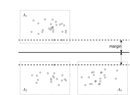
Fig. 2 shows a two dimensional and two-class example to illustrate the difference between the ideas of MMC and M3C (or the other geometric clustering methods). In this example, all the trajectory data are distributed in areas A1subscript𝐴1A_{1}, A2subscript𝐴2A_{2} and A3subscript𝐴3A_{3}, and A1subscript𝐴1A_{1} is far away from A2subscript𝐴2A_{2} and A3subscript𝐴3A_{3}. As shown in Fig. 2a, the optimal decision boundary founded by MMC is a horizontal line for which can achieve the maximum classification margin, and then MMC decomposes the three areas as {A1}{A2,A3}subscript𝐴1subscript𝐴2subscript𝐴3\{A_{1}\}\cup\{A_{2},A_{3}\}. Fig. 2b displays both data points and trajectories. As can be seen, the MMC decomposition severely violates the large margin metastable constraint because of the existence of frequent switches between A1subscript𝐴1A_{1} and A2subscript𝐴2A_{2} in trajectories, and the optimal decomposition provided by M3C (with an appropriate class balance constraint) is then {A1,A2}{A3}subscript𝐴1subscript𝐴2subscript𝐴3\{A_{1},A_{2}\}\cup\{A_{3}\}. Obviously, the decomposition result of M3C is more reasonable from the view of metastability analysis. From this example we can observe that the M3C method is able to exploit the information on both phase space distribution and metastable dynamics contained in the trajectory data by using the large margin metastable constraint.
Refer to caption
(a) MMC
Refer to caption
(b) M3C
Figure 2: Illustration of decision boundaries obtained by MMC and M3C, where solid lines are decision boundaries, dashed lines show the margins, dash-dot lines represent phase space trajectories, and circles denote data points sampled from the trajectories.

Compared with the kinetic clustering methods of metastable state decomposition (e.g., PCCA+), the M3C method directly minimizes the “loss” caused by boundary crossings between metastable states without an explicit model of the system dynamics. Therefore, plenty of statistical problems which are essential and difficult for kinetic clustering methods, including the choice of space discretization and the estimation of transition probabilities, are not present in M3C. Furthermore, the large margin criterion used in M3C provides a convenient and powerful way to reduce the influence of statistical noise. Although some kinetic clustering methods can also handle the statistical noise in a Bayesian manner (see e.g., [29]), M3C offers the advantage of naturally achieving good performance of generalization and robustness without assuming any prior distribution.

The major challenge of M3C arises from (13), which is a nonconvex mixed-integer optimization problem as the MMC problem (6). Due to the similarity between the MMC and M3C problems, solving of the latter encounters similar difficulties: the SDP relaxation based global search requires a high computational cost and the local search easily gets stuck in poor local optima.

5 Optimization method for metastable maximum margin clustering

In this section, we will propose a coarse graining based strategy to solve the M3C problem (13) that takes advantages of both global search and local search methods, and is applicable to large-scale data sets. The proposed optimization procedure can be sketched in the following steps:

  1. 1.

    Coarse graining. Discretize the space 𝒳×𝒳𝒳𝒳\mathcal{X}\times\mathcal{X} of transition pairs into Ncsuperscript𝑁𝑐N^{c} (κ<NcN𝜅superscript𝑁𝑐much-less-than𝑁\kappa<N^{c}\ll N) bins and approximate 𝒫𝒫\mathcal{P} by a coarse-grained data set 𝒫c={(𝐱¯nc,𝐱¯nc)}n=1Ncsuperscript𝒫𝑐superscriptsubscriptsuperscriptsubscript¯𝐱𝑛𝑐superscriptsubscript¯𝐱𝑛𝑐𝑛1superscript𝑁𝑐\mathcal{P}^{c}=\{(\bar{\mathbf{x}}_{n}^{c},\underaccent{\bar}{\mathbf{x}}_{n}^{c})\}_{n=1}^{N^{c}} with normalized weights {cn}subscript𝑐𝑛\{c_{n}\}, where (𝐱¯nc,𝐱¯nc)superscriptsubscript¯𝐱𝑛𝑐superscriptsubscript¯𝐱𝑛𝑐(\bar{\mathbf{x}}_{n}^{c},\underaccent{\bar}{\mathbf{x}}_{n}^{c}) denotes the center of the n𝑛n-th bin and cnsubscript𝑐𝑛c_{n} is proportional to the number of transition pairs contained in the n𝑛n-th bin. This step can be done by k𝑘k-means, k𝑘k-medoids or any other traditional clustering algorithm, and the value of Ncsuperscript𝑁𝑐N^{c} is chosen based on the limitation of computational resources.

  2. 2.

    Global search. Perform M3C on the coarse-grained data set 𝒫csuperscript𝒫𝑐\mathcal{P}^{c} by using the SDP relaxation method. Note that 𝒫csuperscript𝒫𝑐\mathcal{P}^{c} only has a small number of distinct elements, then a satisfactory solution can be achieved in this step without too much computing burden.

  3. 3.

    Local search. Refine the solution obtained in the global search step by applying some local search algorithm to the M3C problem on 𝒫𝒫\mathcal{P}. Here we select the alternating optimization presented in [43] to perform the local search because it is computationally efficient and can handle the class balance constraint easily.

Below we will discuss the last two steps in more detail.

5.1 Global search

For convenience of analysis and computation, we confine that all decision hyperplanes pass through the origin in the feature space, i.e., b1==bκ=0subscript𝑏1subscript𝑏𝜅0b_{1}=\ldots=b_{\kappa}=0. (This is a mild restriction especially for high dimensional feature spaces, since it reduces the number of freedom degrees of decision hyperplanes only by one.) Then the M3C problem on 𝒫csuperscript𝒫𝑐\mathcal{P}^{c} can be expressed as

min𝐲c,𝐖,𝝃c12β𝐖2+𝐜𝝃cs.t.n=1,,Nc,k¯,k¯=1,,κ,(𝐰yncync𝐰k¯k¯)ϕ(𝐱¯nc,𝐱¯nc)+1ync=k¯=k¯1ξnc,ϱlm=1Nc1ymc=k¯cmϱu.subscriptsuperscript𝐲𝑐𝐖superscript𝝃𝑐12𝛽superscriptnorm𝐖2superscript𝐜superscript𝝃𝑐formulae-sequencestformulae-sequencefor-all𝑛1superscript𝑁𝑐for-all¯𝑘¯𝑘1𝜅missing-subexpressionsuperscriptsubscript𝐰superscriptsubscript𝑦𝑛𝑐superscriptsubscript𝑦𝑛𝑐superscriptsubscript𝐰¯𝑘¯𝑘bold-italic-ϕsuperscriptsubscript¯𝐱𝑛𝑐superscriptsubscript¯𝐱𝑛𝑐subscript1superscriptsubscript𝑦𝑛𝑐¯𝑘¯𝑘1superscriptsubscript𝜉𝑛𝑐missing-subexpressionsubscriptitalic-ϱ𝑙superscriptsubscript𝑚1superscript𝑁𝑐subscript1superscriptsubscript𝑦𝑚𝑐¯𝑘subscript𝑐𝑚subscriptitalic-ϱ𝑢\begin{array}[]{cl}\min\limits_{\mathbf{y}^{c},\mathbf{W},\bm{\xi}^{c}}&\frac{1}{2}\beta\left\|\mathbf{W}\right\|^{2}+\mathbf{c}^{\intercal}\bm{\xi}^{c}\\ \mathrm{s.t.}&\forall n=1,\ldots,N^{c},\quad\forall\bar{k},\underaccent{\bar}{k}=1,\ldots,\kappa,\\ &\left(\mathbf{w}_{y_{n}^{c}y_{n}^{c}}^{\intercal}-\mathbf{w}_{\bar{k}\underaccent{\bar}{k}}^{\intercal}\right)\bm{\phi}\left(\bar{\mathbf{x}}_{n}^{c},\underaccent{\bar}{\mathbf{x}}_{n}^{c}\right)+1_{y_{n}^{c}=\bar{k}=\underaccent{\bar}{k}}\geq 1-\xi_{n}^{c},\\ &\varrho_{l}\leq\sum_{m=1}^{N^{c}}1_{y_{m}^{c}=\bar{k}}\cdot c_{m}\leq\varrho_{u}.\end{array} (14)

where ync{1,,κ}superscriptsubscript𝑦𝑛𝑐1𝜅y_{n}^{c}\in\{1,\ldots,\kappa\} and ξncsuperscriptsubscript𝜉𝑛𝑐\xi_{n}^{c} denotes the label and slack variable of the n𝑛n-th coarse-grained transition pair (𝐱¯nc,𝐱¯nc)superscriptsubscript¯𝐱𝑛𝑐superscriptsubscript¯𝐱𝑛𝑐(\bar{\mathbf{x}}_{n}^{c},\underaccent{\bar}{\mathbf{x}}_{n}^{c}), 𝐲c=(y1c,,yNcc)superscript𝐲𝑐superscriptsubscript𝑦1𝑐superscriptsubscript𝑦superscript𝑁𝑐𝑐\mathbf{y}^{c}=(y_{1}^{c},\ldots,y_{N^{c}}^{c}), 𝝃c=(ξ1c,,ξNcc)superscript𝝃𝑐superscriptsuperscriptsubscript𝜉1𝑐superscriptsubscript𝜉superscript𝑁𝑐𝑐\bm{\xi}^{c}=(\xi_{1}^{c},\ldots,\xi_{N^{c}}^{c})^{\intercal}, and 𝐜=(c1,,cNc)𝐜superscriptsubscript𝑐1subscript𝑐superscript𝑁𝑐\mathbf{c}=(c_{1},\ldots,c_{N^{c}})^{\intercal} denotes the vector of weights of coarse-grained transition pairs. It is clear that the assignment 𝐲csuperscript𝐲𝑐\mathbf{y}^{c} in (14) can be represented by the equivalence relation matrices 𝐃Nc×κ𝐃superscriptsuperscript𝑁𝑐𝜅\mathbf{D}\in\mathbb{R}^{N^{c}\times\kappa} and 𝐌Nc×Nc𝐌superscriptsuperscript𝑁𝑐superscript𝑁𝑐\mathbf{M}\in\mathbb{R}^{N^{c}\times N^{c}} which are defined by

𝐃=[Dij]=[1yic=j],𝐌=[Mij]=[1yic=yjc]formulae-sequence𝐃delimited-[]subscript𝐷𝑖𝑗delimited-[]subscript1superscriptsubscript𝑦𝑖𝑐𝑗𝐌delimited-[]subscript𝑀𝑖𝑗delimited-[]subscript1superscriptsubscript𝑦𝑖𝑐superscriptsubscript𝑦𝑗𝑐\mathbf{D}=[D_{ij}]=[1_{y_{i}^{c}=j}],\quad\mathbf{M}=[M_{ij}]=[1_{y_{i}^{c}=y_{j}^{c}}] (15)

i.e., the (i,j)𝑖𝑗(i,j)-th element of 𝐃𝐃\mathbf{D} indicates if the label of (𝐱¯ic,𝐱¯ic)superscriptsubscript¯𝐱𝑖𝑐superscriptsubscript¯𝐱𝑖𝑐(\bar{\mathbf{x}}_{i}^{c},\underaccent{\bar}{\mathbf{x}}_{i}^{c}) is j𝑗j, and the (i,j)𝑖𝑗(i,j)-th element of 𝐌𝐌\mathbf{M} indicates if (𝐱¯ic,𝐱¯ic)superscriptsubscript¯𝐱𝑖𝑐superscriptsubscript¯𝐱𝑖𝑐(\bar{\mathbf{x}}_{i}^{c},\underaccent{\bar}{\mathbf{x}}_{i}^{c}) and (𝐱¯jc,𝐱¯jc)superscriptsubscript¯𝐱𝑗𝑐superscriptsubscript¯𝐱𝑗𝑐(\bar{\mathbf{x}}_{j}^{c},\underaccent{\bar}{\mathbf{x}}_{j}^{c}) are assigned to the same label.

Replacing 𝐲csuperscript𝐲𝑐\mathbf{y}^{c} by (𝐌,𝐃)𝐌𝐃(\mathbf{M},\mathbf{D}) as assignment variables in (14) and using the strong duality theorem, we can get an equivalent form of the coarse-grained M3C problem.

Theorem 5.

Solving (14) is equivalent to solving the optimization problem

min𝐌,𝐃,𝜶,𝜽12𝜽𝜽𝐜𝜶12βtr(𝐌𝐂𝐊s𝐂)+𝟏𝐜s.t.𝐪(𝐃)+(𝟏𝐈)𝜶+𝐑𝜽0,ϱl𝐌𝐜ϱu,diag(𝐌)=𝟏,𝐌=𝐃𝐃,𝐌{0,1}Nc×Nc,𝐃{0,1}Nc×κ.subscript𝐌𝐃𝜶𝜽12superscript𝜽𝜽superscript𝐜𝜶12𝛽trsuperscript𝐌𝐂𝐊𝑠𝐂superscript1𝐜formulae-sequencest𝐪𝐃tensor-product1𝐈𝜶𝐑𝜽0missing-subexpressionsubscriptitalic-ϱ𝑙𝐌𝐜subscriptitalic-ϱ𝑢missing-subexpressiondiag𝐌1missing-subexpression𝐌superscript𝐃𝐃missing-subexpressionformulae-sequence𝐌superscript01superscript𝑁𝑐superscript𝑁𝑐𝐃superscript01superscript𝑁𝑐𝜅\begin{array}[]{cl}\min\limits_{\mathbf{M},\mathbf{D},\bm{\alpha},\bm{\theta}}&\frac{1}{2}\bm{\theta}^{\intercal}\bm{\theta}-\mathbf{c}^{\intercal}\bm{\alpha}-\frac{1}{2\beta}\mathrm{tr}\left(\mathbf{M}\mathbf{C}\mathbf{K}^{s}\mathbf{C}\right)+\mathbf{1}^{\intercal}\mathbf{c}\\ \mathrm{s.t.}&\mathbf{q}\left(\mathbf{D}\right)+\left(\mathbf{1}\otimes\mathbf{I}\right)\bm{\alpha}+\mathbf{R}\bm{\theta}\leq 0,\\ &\varrho_{l}\leq\mathbf{M}\mathbf{c}\leq\varrho_{u},\\ &\mathrm{diag}\left(\mathbf{M}\right)=\mathbf{1},\\ &\mathbf{M}=\mathbf{D}\mathbf{D}^{\intercal},\\ &\mathbf{M}\in\left\{0,1\right\}^{N^{c}\times N^{c}},\mathbf{D}\in\left\{0,1\right\}^{N^{c}\times\kappa}.\end{array} (16)

where 𝐂𝐂\mathbf{C} is a diagonal matrix with the elements of 𝐜𝐜\mathbf{c} on the diagonal, 𝐪(𝐃)𝐪𝐃\mathbf{q}\left(\mathbf{D}\right) is a linear function of 𝐃𝐃\mathbf{D} defined in (47), and definitions of 𝐊ssuperscript𝐊𝑠\mathbf{K}^{s} and 𝐑𝐑\mathbf{R} are given by (42) and (49).

Proof.

See B.∎

Remark 6.

The last four constraints on 𝐌𝐌\mathbf{M} and 𝐃𝐃\mathbf{D} of (16) come from the fact that there is a 𝐲csuperscript𝐲𝑐\mathbf{y}^{c} such that (15) holds if and only if 𝐌𝐌\mathbf{M} and 𝐃𝐃\mathbf{D} are both binary matrices and satisfy diag(𝐌)=𝟏diag𝐌1\mathrm{diag}\left(\mathbf{M}\right)=\mathbf{1} and 𝐌=𝐃𝐃𝐌superscript𝐃𝐃\mathbf{M}=\mathbf{D}\mathbf{D}^{\intercal} [34].

It is easy to see that (16) is a convex optimization problem if we drop the constraints that 𝐌𝐌\mathbf{M} and 𝐃𝐃\mathbf{D} are binary matrices and the nonlinear constraint 𝐌=𝐃𝐃𝐌superscript𝐃𝐃\mathbf{M}=\mathbf{D}\mathbf{D}^{\intercal}. This motivates an approximation method for solving the coarse-grained M3C problem based on two relaxations as in [34]. The first relaxation allows elements of 𝐌𝐌\mathbf{M} and 𝐃𝐃\mathbf{D} to take values in [0,1]01[0,1] instead of {0,1}01\{0,1\} and the second relaxation is to replace 𝐌=𝐃𝐃𝐌superscript𝐃𝐃\mathbf{M}=\mathbf{D}\mathbf{D}^{\intercal} with a convex inequality 𝐌𝐃𝐃succeeds-or-equals𝐌superscript𝐃𝐃\mathbf{M}\succeq\mathbf{D}\mathbf{D}^{\intercal}. By using these two relaxations, (16) can be relaxed to a convex optimization problem:

min𝐌,𝐃,𝜶,𝜽12𝜽𝜽𝐜𝜶12βtr(𝐌𝐂𝐊s𝐂)+𝟏𝐜s.t.𝐪(𝐃)+(𝟏𝐈)𝜶+𝐑𝜽0,ϱl𝐌𝐜ϱu,diag(𝐌)=𝟏,𝐌𝐃𝐃,0𝐌1,0𝐃1.subscript𝐌𝐃𝜶𝜽12superscript𝜽𝜽superscript𝐜𝜶12𝛽trsuperscript𝐌𝐂𝐊𝑠𝐂superscript1𝐜formulae-sequencest𝐪𝐃tensor-product1𝐈𝜶𝐑𝜽0missing-subexpressionsubscriptitalic-ϱ𝑙𝐌𝐜subscriptitalic-ϱ𝑢missing-subexpressiondiag𝐌1missing-subexpressionsucceeds-or-equals𝐌superscript𝐃𝐃missing-subexpressionformulae-sequence0𝐌10𝐃1\begin{array}[]{cl}\min\limits_{\mathbf{M},\mathbf{D},\bm{\alpha},\bm{\theta}}&\frac{1}{2}\bm{\theta}^{\intercal}\bm{\theta}-\mathbf{c}^{\intercal}\bm{\alpha}-\frac{1}{2\beta}\mathrm{tr}\left(\mathbf{M}\mathbf{C}\mathbf{K}^{s}\mathbf{C}\right)+\mathbf{1}^{\intercal}\mathbf{c}\\ \mathrm{s.t.}&\mathbf{q}\left(\mathbf{D}\right)+\left(\mathbf{1}\otimes\mathbf{I}\right)\bm{\alpha}+\mathbf{R}\bm{\theta}\leq 0,\\ &\varrho_{l}\leq\mathbf{M}\mathbf{c}\leq\varrho_{u},\\ &\mathrm{diag}\left(\mathbf{M}\right)=\mathbf{1},\\ &\mathbf{M}\succeq\mathbf{D}\mathbf{D}^{\intercal},\\ &0\leq\mathbf{M}\leq 1,0\leq\mathbf{D}\leq 1.\end{array} (17)

According to the Schur complement lemma [47], we can further reformulate (17) in a more convenient form:

min𝐌,𝐃,𝜶,𝜽,ζζs.t.[𝐈𝜽𝜽2(ζ+𝐜𝜶+12βtr(𝐌𝐂𝐊s𝐂)𝟏𝐜)]0,𝐪(𝐃)+(𝟏𝐈)𝜶+𝐑𝜽0,ϱl𝐌𝐜ϱu,diag(𝐌)=𝟏,[𝐈𝐃𝐃𝐌]0,0𝐌1,0𝐃1.subscript𝐌𝐃𝜶𝜽𝜁𝜁formulae-sequencestsucceeds-or-equalsdelimited-[]𝐈𝜽superscript𝜽2𝜁superscript𝐜𝜶12𝛽trsuperscript𝐌𝐂𝐊𝑠𝐂superscript1𝐜0missing-subexpression𝐪𝐃tensor-product1𝐈𝜶𝐑𝜽0missing-subexpressionsubscriptitalic-ϱ𝑙𝐌𝐜subscriptitalic-ϱ𝑢missing-subexpressiondiag𝐌1missing-subexpressionsucceeds-or-equalsdelimited-[]𝐈superscript𝐃𝐃𝐌0missing-subexpressionformulae-sequence0𝐌10𝐃1\begin{array}[]{cl}\min\limits_{\mathbf{M},\mathbf{D},\bm{\alpha},\bm{\theta},\zeta}&\zeta\\ \mathrm{s.t.}&\left[\begin{array}[]{cc}\mathbf{I}&\bm{\theta}\\ \bm{\theta}^{\intercal}&2\left(\zeta+\mathbf{c}^{\intercal}\bm{\alpha}+\frac{1}{2\beta}\mathrm{tr}\left(\mathbf{M}\mathbf{C}\mathbf{K}^{s}\mathbf{C}\right)-\mathbf{1}^{\intercal}\mathbf{c}\right)\end{array}\right]\succeq 0,\\ &\mathbf{q}\left(\mathbf{D}\right)+\left(\mathbf{1}\otimes\mathbf{I}\right)\bm{\alpha}+\mathbf{R}\bm{\theta}\leq 0,\\ &\varrho_{l}\leq\mathbf{M}\mathbf{c}\leq\varrho_{u},\\ &\mathrm{diag}\left(\mathbf{M}\right)=\mathbf{1},\\ &\left[\begin{array}[]{cc}\mathbf{I}&\mathbf{D}^{\intercal}\\ \mathbf{D}&\mathbf{M}\end{array}\right]\succeq 0,\\ &0\leq\mathbf{M}\leq 1,0\leq\mathbf{D}\leq 1.\end{array} (18)

It is an SDP problem and can be solved in polynomial time.

Since the optimal 𝐌𝐌\mathbf{M} obtained from (18) is a symmetric matrix satisfying diag(𝐌)=𝟏diag𝐌1\mathrm{diag}\left(\mathbf{M}\right)=\mathbf{1} and 0𝐌10𝐌10\leq\mathbf{M}\leq 1, it can be interpreted as a similarity matrix of 𝒫csuperscript𝒫𝑐\mathcal{P}^{c} with each element Mijsubscript𝑀𝑖𝑗M_{ij} representing some measure of the similarity between (𝐱¯ic,𝐱¯ic)superscriptsubscript¯𝐱𝑖𝑐superscriptsubscript¯𝐱𝑖𝑐(\bar{\mathbf{x}}_{i}^{c},\underaccent{\bar}{\mathbf{x}}_{i}^{c}) and (𝐱¯jc,𝐱¯jc)superscriptsubscript¯𝐱𝑗𝑐superscriptsubscript¯𝐱𝑗𝑐(\bar{\mathbf{x}}_{j}^{c},\underaccent{\bar}{\mathbf{x}}_{j}^{c}). Hence, we can utilize the spectral clustering method to recover 𝐲csuperscript𝐲𝑐\mathbf{y}^{c} from the optimal 𝐌𝐌\mathbf{M} such that Mij=1yic=yjcsubscript𝑀𝑖𝑗subscript1superscriptsubscript𝑦𝑖𝑐superscriptsubscript𝑦𝑗𝑐M_{ij}=1_{y_{i}^{c}=y_{j}^{c}} approximately holds for all i,j𝑖𝑗i,j.

Remark 7.

Obviously, the relaxation method proposed in this section can be directly applied to the original M3C problem (13) without any coarse graining, and the corresponding relaxed problem can be solved even in the case that we do not know the feature mapping implicitly but only know the kernel function Ker(,)Ker\mathrm{Ker}\left(\cdot,\cdot\right). However, this scheme is generally computationally infeasible because the it involves an SDP problem with O(N2)𝑂superscript𝑁2O(N^{2}) parameters.

5.2 Local search

We now investigate how to refine the clustering result obtained in the global search by local search. A natural way to do this is to alternatively minimize (13) with respect to (𝐖,𝐛)𝐖𝐛\left(\mathbf{W},\mathbf{b}\right) keeping 𝐲𝐲\mathbf{y} fixed and vice versa until convergence, where the initial value of 𝐲𝐲\mathbf{y} is given by the coarse-grained label assignment 𝐲csuperscript𝐲𝑐\mathbf{y}^{c} with

yn=yic, if (𝐱¯n,𝐱¯n) is in the bin centered at (𝐱¯ic,𝐱¯ic)subscript𝑦𝑛superscriptsubscript𝑦𝑖𝑐 if subscript¯𝐱𝑛subscript¯𝐱𝑛 is in the bin centered at superscriptsubscript¯𝐱𝑖𝑐superscriptsubscript¯𝐱𝑖𝑐y_{n}=y_{i}^{c},\text{ if }(\bar{\mathbf{x}}_{n},\underaccent{\bar}{\mathbf{x}}_{n})\text{ is in the bin centered at }(\bar{\mathbf{x}}_{i}^{c},\underaccent{\bar}{\mathbf{x}}_{i}^{c}) (19)

Note that the M3C problem (13) with a fixed 𝐲𝐲\mathbf{y} is just a standard quadratic programming problem. Here we only discuss the optimization problem with respect to 𝐲𝐲\mathbf{y}. For fixed 𝐖𝐖\mathbf{W} and 𝐛𝐛\mathbf{b}, (13) is reduced to

min𝐲𝟏𝝃s.t.n=1,,N,k¯,k¯=1,,κ,(𝐰ynyn𝐰k¯k¯)ϕ(𝐱¯n,𝐱¯n)+(bynynbk¯k¯)+1yn=k¯=k¯1ξn,ϱlNm=1N1ym=k¯ϱuN.subscript𝐲superscript1𝝃formulae-sequencestformulae-sequencefor-all𝑛1𝑁for-all¯𝑘¯𝑘1𝜅missing-subexpressionsuperscriptsubscript𝐰subscript𝑦𝑛subscript𝑦𝑛superscriptsubscript𝐰¯𝑘¯𝑘bold-italic-ϕsubscript¯𝐱𝑛subscript¯𝐱𝑛missing-subexpressionsubscript𝑏subscript𝑦𝑛subscript𝑦𝑛subscript𝑏¯𝑘¯𝑘subscript1subscript𝑦𝑛¯𝑘¯𝑘1subscript𝜉𝑛missing-subexpressionsubscriptitalic-ϱ𝑙𝑁superscriptsubscript𝑚1𝑁subscript1subscript𝑦𝑚¯𝑘subscriptitalic-ϱ𝑢𝑁\begin{array}[]{cl}\min\limits_{\mathbf{y}}&\mathbf{1}^{\intercal}\bm{\xi}\\ \mathrm{s.t.}&\forall n=1,\ldots,N,\quad\forall\bar{k},\underaccent{\bar}{k}=1,\ldots,\kappa,\\ &\left(\mathbf{w}_{y_{n}y_{n}}^{\intercal}-\mathbf{w}_{\bar{k}\underaccent{\bar}{k}}^{\intercal}\right)\bm{\phi}\left(\bar{\mathbf{x}}_{n},\underaccent{\bar}{\mathbf{x}}_{n}\right)\\ &+\left(b_{y_{n}y_{n}}-b_{\bar{k}\underaccent{\bar}{k}}\right)+1_{y_{n}=\bar{k}=\underaccent{\bar}{k}}\geq 1-\xi_{n},\\ &\varrho_{l}N\leq\sum_{m=1}^{N}1_{y_{m}=\bar{k}}\leq\varrho_{u}N.\end{array} (20)

It is simple to verify that (20) can be transformed into a binary linear programming problem

min𝐃ftr(𝐇𝐃f)s.t.ϱlN𝟏𝐃fϱuN,𝐃f{0,1}N×κ.subscriptsuperscript𝐃𝑓trsuperscript𝐇superscript𝐃𝑓formulae-sequencestsubscriptitalic-ϱ𝑙𝑁superscript1superscript𝐃𝑓subscriptitalic-ϱ𝑢𝑁missing-subexpressionsuperscript𝐃𝑓superscript01𝑁𝜅\begin{array}[]{cl}\min\limits_{\mathbf{D}^{f}}&\mathrm{tr}\left(\mathbf{H}^{\intercal}\mathbf{D}^{f}\right)\\ \mathrm{s.t.}&\varrho_{l}N\leq\mathbf{1^{\intercal}}\mathbf{D}^{f}\leq\varrho_{u}N,\\ &\mathbf{D}^{f}\in\left\{0,1\right\}^{N\times\kappa}.\end{array} (21)

where 𝐃f=[Dijf]superscript𝐃𝑓delimited-[]superscriptsubscript𝐷𝑖𝑗𝑓\mathbf{D}^{f}=[D_{ij}^{f}] is a relation matrix with Dijf=1yi=jsuperscriptsubscript𝐷𝑖𝑗𝑓subscript1subscript𝑦𝑖𝑗D_{ij}^{f}=1_{y_{i}=j}, and 𝐇=[Hij]𝐇delimited-[]subscript𝐻𝑖𝑗\mathbf{H}=[H_{ij}] is defined by

Hij=maxk¯,k¯11j=k¯=k¯(𝐰jj𝐰k¯k¯)ϕ(𝐱¯i,𝐱¯i)(bjjbk¯k¯)subscript𝐻𝑖𝑗subscript¯𝑘¯𝑘1subscript1𝑗¯𝑘¯𝑘superscriptsubscript𝐰𝑗𝑗superscriptsubscript𝐰¯𝑘¯𝑘bold-italic-ϕsubscript¯𝐱𝑖subscript¯𝐱𝑖subscript𝑏𝑗𝑗subscript𝑏¯𝑘¯𝑘H_{ij}=\max_{\bar{k},\underaccent{\bar}{k}}1-1_{j=\bar{k}=\underaccent{\bar}{k}}-\left(\mathbf{w}_{jj}^{\intercal}-\mathbf{w}_{\bar{k}\underaccent{\bar}{k}}^{\intercal}\right)\bm{\phi}\left(\bar{\mathbf{x}}_{i},\underaccent{\bar}{\mathbf{x}}_{i}\right)-\left(b_{jj}-b_{\bar{k}\underaccent{\bar}{k}}\right) (22)

Although (21) belongs to the class of NP-hard problems, it can be efficiently tackled by enumeration and cutting-plane techniques [48] in practice, and there exist a lot of software packages for solving large-scale integer programming problems like (21), including MOSEK [49], Gurobi [50] and GLPK [51].

Remark 8.

It was reported in [43] that the alternating optimization method for MMC often suffers from premature convergence and can only change a small proportion of data labels even with a poor initialization, but our numerical experiments show that this problem is not serious for the local search procedure of M3C. The analysis of this phenomenon requires further investigation and we only give a rough explanation here. Generally speaking, the switching between metastable states can be observed many times in trajectories. Therefore, during the local search of M3C, there are always a number of transition pairs that are close to the decision boundaries and violate the large margin metastable constraint with not-so-small slack values even if β1much-less-than𝛽1\beta\ll 1. These misclassified transition pairs are helpful to “push” the decision boundaries away from the initial positions and their labels can be easily changed especially in early iterations of the local search.

5.3 Full description of the optimization procedure

Based on the above analysis, the complete optimization method developed for M3C can be summarized in Algorithm 1.

1:  generate a coarse-grained transition pair set 𝒫csuperscript𝒫𝑐\mathcal{P}^{c} with cardinality Ncsuperscript𝑁𝑐N^{c} and normalized weights 𝐜=(c1,,cNc)𝐜superscriptsubscript𝑐1subscript𝑐superscript𝑁𝑐\mathbf{c}=(c_{1},\ldots,c_{N^{c}})^{\intercal} from 𝒫𝒫\mathcal{P} by the k𝑘k-means or k𝑘k-medoids algorithm
2:  find (𝐌,𝐃)superscript𝐌superscript𝐃(\mathbf{M}^{*},\mathbf{D}^{*}) as the solution to the SDP problem (18)
3:  perform the spectral clustering algorithm with similarity matrix 𝐌superscript𝐌\mathbf{M}^{*} to get class labels 𝐲c=(y1c,,yNcc)superscript𝐲𝑐superscriptsubscript𝑦1𝑐superscriptsubscript𝑦superscript𝑁𝑐𝑐\mathbf{y}^{c}=(y_{1}^{c},\ldots,y_{N^{c}}^{c}) of coarse-grained transition pairs in 𝒫csuperscript𝒫𝑐\mathcal{P}^{c}
4:  calculate class labels 𝐲=(y1,,yN)𝐲subscript𝑦1subscript𝑦𝑁\mathbf{y}=(y_{1},\ldots,y_{N}) of transition pairs in 𝒫𝒫\mathcal{P} from 𝐲csuperscript𝐲𝑐\mathbf{y}^{c} by (19)
5:  initialize with 𝐲(0)=𝐲superscript𝐲0𝐲\mathbf{y}^{(0)}=\mathbf{y} and r=1𝑟1r=1
6:  repeat
7:     find (𝐖,𝐛)superscript𝐖superscript𝐛(\mathbf{W}^{*},\mathbf{b}^{*}) as the solution to the quadratic programming problem (13) with 𝐲𝐲\mathbf{y} fixed to be 𝐲(r1)superscript𝐲𝑟1\mathbf{y}^{(r-1)} and set (𝐖(r),𝐛(r))=(𝐖,𝐛)superscript𝐖𝑟superscript𝐛𝑟superscript𝐖superscript𝐛(\mathbf{W}^{(r)},\mathbf{b}^{(r)})=(\mathbf{W}^{*},\mathbf{b}^{*})
8:     find 𝐃f=[Dijf]superscript𝐃𝑓delimited-[]superscriptsubscript𝐷𝑖𝑗𝑓\mathbf{D}^{f*}=[D_{ij}^{f*}] as the solution to the binary linear programming problem (21) with (𝐖,𝐛)𝐖𝐛(\mathbf{W},\mathbf{b}) set to be (𝐖(r),𝐛(r))superscript𝐖𝑟superscript𝐛𝑟(\mathbf{W}^{(r)},\mathbf{b}^{(r)}).
9:     calculate 𝐲=(y1,,yN)superscript𝐲superscriptsubscript𝑦1superscriptsubscript𝑦𝑁\mathbf{y}^{*}=(y_{1}^{*},\ldots,y_{N}^{*}) by yn=argmaxjDnjfsuperscriptsubscript𝑦𝑛subscriptargmax𝑗superscriptsubscript𝐷𝑛𝑗𝑓y_{n}^{*}=\mathop{\mathrm{argmax}}_{j}D_{nj}^{f*} and set 𝐲(r)=𝐲superscript𝐲𝑟superscript𝐲\mathbf{y}^{(r)}=\mathbf{y}^{*}
10:     set r:=r+1assign𝑟𝑟1r:=r+1
11:  until the Hamming distance between 𝐲(r)superscript𝐲𝑟\mathbf{y}^{(r)} and 𝐲(r1)superscript𝐲𝑟1\mathbf{y}^{(r-1)} is less than or equal to a given constant αHsubscript𝛼𝐻\alpha_{H} or r𝑟r is larger than a pre-defined threshold rmaxsubscript𝑟r_{\max}
12:  return  (𝐖(r),𝐛(r),𝐲(r))superscript𝐖𝑟superscript𝐛𝑟superscript𝐲𝑟(\mathbf{W}^{(r)},\mathbf{b}^{(r)},\mathbf{y}^{(r)})
Algorithm 1 Optimization procedure for M3C

6 Experiments

In this section, we demonstrate the performance of the proposed decomposition method on some synthetic metastable systems and molecular dynamics simulations.

The detailed settings of Algorithm 1 for M3C are as follows:

  • 1.

    In the coarse graining step, 𝒫csuperscript𝒫𝑐\mathcal{P}^{c} is provided by the standard k𝑘k-medoids algorithm [52] with Nc=30superscript𝑁𝑐30N^{c}=30. (Here we use k𝑘k-medoids rather than k𝑘k-means because k𝑘k-medoids is more robust to outliers and can avoid the appearance of the coarse-grained transitions which make no physical sense.)

  • 2.

    All the involved SDP problems and the binary linear programming problem (21) are solved by using the Mosek solver [49] through the CVX interface in Matlab [53].

  • 3.

    The spectral clustering algorithm proposed in [54] is utilized to extract 𝐲csuperscript𝐲𝑐\mathbf{y}^{c} from the relation matrix 𝐌𝐌\mathbf{M}.

  • 4.

    The feature mapping ϕ()bold-italic-ϕ\bm{\phi}\left(\cdot\right) is induced from the Gaussian kernel

    Ker(𝐱,𝐱)=exp(𝐱𝐱22σ2)Ker𝐱superscript𝐱superscriptnorm𝐱superscript𝐱22superscript𝜎2\mathrm{Ker}\left(\mathbf{x},\mathbf{x}^{\prime}\right)=\exp\left(-\frac{\left\|\mathbf{x}-\mathbf{x}^{\prime}\right\|^{2}}{2\sigma^{2}}\right) (23)

    and explicitly computed by the random Fourier method [44] with d=50𝑑50d=50. The width parameter σ𝜎\sigma is determined by a grid search over {24,23,,24}superscript24superscript23superscript24\{2^{-4},2^{-3},\ldots,2^{4}\} and we select the value of σ𝜎\sigma which leads to the minimal value of the objective function of the M3C problem (13).

  • 5.

    The value of regularization parameter β𝛽\beta does not have a significant effect for our experiments, so it is simply fixed to 0.010.010.01.

  • 6.

    The parameters of termination condition are set to be αH=0subscript𝛼𝐻0\alpha_{H}=0 and rmax=100subscript𝑟100r_{\max}=100, and the parameters of class balance constraint are (ϱl,ϱu)=(0.01,0.99)subscriptitalic-ϱ𝑙subscriptitalic-ϱ𝑢0.010.99\left(\varrho_{l},\varrho_{u}\right)=\left(0.01,0.99\right).

For comparison purposes, the following three decomposition methods are also considered in our experiments:

  1. 1.

    k𝑘k-medoids clustering, which directly decomposes the phase space into κ𝜅\kappa macrostates based on the set 𝒮={𝐱tl|1lL,1tMl}𝒮conditional-setsuperscriptsubscript𝐱𝑡𝑙formulae-sequence1𝑙𝐿1𝑡subscript𝑀𝑙\mathcal{S}=\{\mathbf{x}_{t}^{l}|1\leq l\leq L,1\leq t\leq M_{l}\}.

  2. 2.

    MMC based on 𝒮𝒮\mathcal{S}, where the MMC problem is solved by a mixed algorithm similar to Algorithm 1 (see C).

  3. 3.

    PCCA+ [26], where the implementation details are given in Appendix D.

Remark 9.

k𝑘k-medoids clustering and MMC can be viewed as geometric clustering methods in metastability analysis.

Remark 10.

Considering the inherent randomness of the k𝑘k-medoids algorithm, here we perform the k𝑘k-medoids clustering (or k𝑘k-medoids clustering in coarse graining steps of MMC, PCCA+ and M3C ) in the following way: Repeat the k𝑘k-medoids algorithm 100100100 times independently with random initialization and pick the solution with the minimal “within-cluster point scatter”.

6.1 Sequential unlabeled data

Here we apply M3C and other metastable state decomposition methods to sequential data which are generated by using data sets letter, satellite, spambase, waveform and segment from the UCI machine learning repository [55]. All data sets consist of multiple classes of instances and the pattern of each instance is represented by a multidimensional vector of real- or integer-valued features. A summary of all the data sets is in Table 1.

For each data set, we construct a sequence of unlabeled patterns as follows:

  1. 1.

    Generate a reversible Markov chain {y¯n}n=1Nsuperscriptsubscriptsubscript¯𝑦𝑛𝑛1𝑁\{\bar{y}_{n}\}_{n=1}^{N} in {1,,κ}1𝜅\{1,\ldots,\kappa\}, where κ𝜅\kappa denotes the class number of the data set, and the transition matrix 𝐏=[Pij]=[Pr(y¯n+1=j|y¯n=i)]κ×κ𝐏delimited-[]subscript𝑃𝑖𝑗delimited-[]Prsubscript¯𝑦𝑛1conditional𝑗subscript¯𝑦𝑛𝑖superscript𝜅𝜅\mathbf{P}=[P_{ij}]=[\Pr(\bar{y}_{n+1}=j|\bar{y}_{n}=i)]\in\mathbb{R}^{\kappa\times\kappa} of {y¯n}subscript¯𝑦𝑛\{\bar{y}_{n}\} is given by

    𝐏𝐏\displaystyle\mathbf{P} =\displaystyle= [0.970.030.030.97]delimited-[]0.970.030.030.97\displaystyle\left[\begin{array}[]{cc}0.97&0.03\\ 0.03&0.97\end{array}\right]
    𝐏𝐏\displaystyle\mathbf{P} =\displaystyle= [0.970.0150.0150.0250.950.0250.020.020.96]delimited-[]0.970.0150.0150.0250.950.0250.020.020.96\displaystyle\left[\begin{array}[]{ccc}0.97&0.015&0.015\\ 0.025&0.95&0.025\\ 0.02&0.02&0.96\end{array}\right]
    𝐏𝐏\displaystyle\mathbf{P} =\displaystyle= [0.95170.01980.01380.01470.01980.95090.01340.01590.01380.01340.95350.01930.01470.01590.01930.9501]delimited-[]0.95170.01980.01380.01470.01980.95090.01340.01590.01380.01340.95350.01930.01470.01590.01930.9501\displaystyle\left[\begin{array}[]{cccc}0.9517&0.0198&0.0138&0.0147\\ 0.0198&0.9509&0.0134&0.0159\\ 0.0138&0.0134&0.9535&0.0193\\ 0.0147&0.0159&0.0193&0.9501\end{array}\right]

    for κ=2,3,4𝜅234\kappa=2,3,4 repsectively.

  2. 2.

    For every n=1,,N𝑛1𝑁n=1,\ldots,N, randomly select a pattern 𝐱nsubscript𝐱𝑛\mathbf{x}_{n} with class label y¯nsubscript¯𝑦𝑛\bar{y}_{n} from the data set without repetition. (This step cannot be implemented if the element number of {n|y¯n=i}conditional-set𝑛subscript¯𝑦𝑛𝑖\{n|\bar{y}_{n}=i\} is bigger than the data size of the i𝑖i-th class in the data set for some i𝑖i. For such a case, we will repeat generating {y¯n}subscript¯𝑦𝑛\{\bar{y}_{n}\} until this step is feasible.)

Since the self-transition probabilities in transition matrices 𝐏𝐏\mathbf{P} (i.e., the diagonal elements of 𝐏𝐏\mathbf{P}) are all close to 111, a pattern sequence {𝐱n}subscript𝐱𝑛\{\mathbf{x}_{n}\} generated as above can be viewed as a metastable processes with each class being a metastable state. Then we perform clustering of {𝐱n}subscript𝐱𝑛\{\mathbf{x}_{n}\} by metastable state decomposition after removing the class labels of {𝐱n}subscript𝐱𝑛\{\mathbf{x}_{n}\}. Finally, the clustering accuracies of different methods are evaluated by calculating classification errors on the training data set {𝐱n}subscript𝐱𝑛\{\mathbf{x}_{n}\} and the testing data set consisting of all instances not in {𝐱n}subscript𝐱𝑛\{\mathbf{x}_{n}\}:

errtrainsubscripterrtrain\displaystyle\mathrm{err}_{\mathrm{train}} =\displaystyle= 1Nn=1N1y¯ny(𝐱n)1𝑁superscriptsubscript𝑛1𝑁subscript1subscript¯𝑦𝑛𝑦subscript𝐱𝑛\displaystyle\frac{1}{N}\sum_{n=1}^{N}1_{\bar{y}_{n}\neq y\left(\mathbf{x}_{n}\right)}
errtestsubscripterrtest\displaystyle\mathrm{err}_{\mathrm{test}} =\displaystyle= 1|{testing data}|𝐱{testing data}1y¯(𝐱)y(𝐱)1testing datasubscript𝐱testing datasubscript1¯𝑦𝐱𝑦𝐱\displaystyle\frac{1}{|\{\text{testing data}\}|}\sum_{\mathbf{x}\in\{\text{testing data}\}}1_{\bar{y}\left(\mathbf{x}\right)\neq y\left(\mathbf{x}\right)} (27)

where y¯(𝐱)¯𝑦𝐱\bar{y}\left(\mathbf{x}\right) denotes the true class label of 𝐱𝐱\mathbf{x}, and y(𝐱)𝑦𝐱y\left(\mathbf{x}\right) denotes the predicted label given by metastable state decomposition results.

Table 2 summarizes clustering errors on the various data sets with N=1000𝑁1000N=1000. It can be observed from the table that both PCCA+ and M3C outperform the geometric clustering methods, k𝑘k-medoids and MMC, by utilizing the metastable structure in the sequential, and M3C achieves the best clustering performance among all the four methods. Moreover, considering that the clustering given by PCCA+ depend on the space discretization results (see Section 1), we report the clustering errors of PCCA+ with different numbers of discrete bins in this table. As can be seen, for most data sets, except segment, either the finest discretization (with 400400400 bins) or the coarsest discretization (with 505050 bins) cannot lead to the best PCCA+ clustering results, which demonstrates the sensitivity of PCCA+ to the choice of space discretization.

Table 1: Summary of the data sets
size pattern dimension number of classesa)  (κ𝜅\kappa)
letter 155515551555 171717 222
satellite 223622362236 363636 222
spambase 460146014601 575757 222
waveform 500050005000 212121 333
segment 132013201320 191919 444
  • a)

    For data sets which contain more than κ𝜅\kappa classes, we only use their subsets consising of the first κ𝜅\kappa classes.

Table 2: Means and standard deviations of clustering errors (in percent) calculated over 202020 independent experiments of various data sets
k𝑘k-medoids MMC PCCA+(50 bins)PCCA+(50 bins)\begin{array}[]{c}\text{PCCA+}\\ \text{(50 bins)}\end{array} PCCA+(200 bins)PCCA+(200 bins)\begin{array}[]{c}\text{PCCA+}\\ \text{(200 bins)}\end{array} PCCA+(300 bins)PCCA+(300 bins)\begin{array}[]{c}\text{PCCA+}\\ \text{(300 bins)}\end{array} PCCA+(400 bins)PCCA+(400 bins)\begin{array}[]{c}\text{PCCA+}\\ \text{(400 bins)}\end{array} M3C
letter errtrainsubscripterrtrain\mathrm{err}_{\mathrm{train}} 8.6306±3.0850plus-or-minus8.63063.08508.6306\pm 3.0850 7.0090±3.2752plus-or-minus7.00903.27527.0090\pm 3.2752 2.2450±1.0128plus-or-minus2.24501.01282.2450\pm 1.0128 0.5450±0.1849plus-or-minus0.54500.18490.5450\pm 0.1849 0.4450±0.2585plus-or-minus0.44500.25850.4450\pm 0.2585 0.5950±0.2837plus-or-minus0.59500.28370.5950\pm 0.2837 0.1100±0.0852plus-or-minus0.11000.0852\mathbf{0.1100\pm 0.0852}
errtestsubscripterrtest\mathrm{err}_{\mathrm{test}} 8.6400±3.0025plus-or-minus8.64003.00258.6400\pm 3.0025 7.3600±3.6059plus-or-minus7.36003.60597.3600\pm 3.6059 2.7207±1.4567plus-or-minus2.72071.45672.7207\pm 1.4567 1.1171±0.5746plus-or-minus1.11710.57461.1171\pm 0.5746 0.7658±0.5871plus-or-minus0.76580.58710.7658\pm 0.5871 1.0270±0.6299plus-or-minus1.02700.62991.0270\pm 0.6299 0.2342±0.1963plus-or-minus0.23420.1963\mathbf{0.2342\pm 0.1963}
satellite errtrainsubscripterrtrain\mathrm{err}_{\mathrm{train}} 2.3503±0.8560plus-or-minus2.35030.85602.3503\pm 0.8560 2.3058±0.8616plus-or-minus2.30580.86162.3058\pm 0.8616 0.7727±0.2905plus-or-minus0.77270.29050.7727\pm 0.2905 0.6600±0.2741plus-or-minus0.66000.27410.6600\pm 0.2741 0.7600±0.2604plus-or-minus0.76000.26040.7600\pm 0.2604 0.8600±0.2501plus-or-minus0.86000.25010.8600\pm 0.2501 0.0900±0.0912plus-or-minus0.09000.0912\mathbf{0.0900\pm 0.0912}
errtestsubscripterrtest\mathrm{err}_{\mathrm{test}} 6.7950±1.3069plus-or-minus6.79501.30696.7950\pm 1.3069 6.6450±1.4365plus-or-minus6.64501.43656.6450\pm 1.4365 1.1950±0.3348plus-or-minus1.19500.33481.1950\pm 0.3348 0.7727±0.3457plus-or-minus0.77270.34570.7727\pm 0.3457 0.9102±0.3803plus-or-minus0.91020.38030.9102\pm 0.3803 1.0720±0.5436plus-or-minus1.07200.54361.0720\pm 0.5436 0.3196±0.1325plus-or-minus0.31960.1325\mathbf{0.3196\pm 0.1325}
spambase errtrainsubscripterrtrain\mathrm{err}_{\mathrm{train}} 36.8773±1.8360plus-or-minus36.87731.836036.8773\pm 1.8360 22.5923±9.7192plus-or-minus22.59239.719222.5923\pm 9.7192 23.6000±9.2388plus-or-minus23.60009.238823.6000\pm 9.2388 25.7450±13.4768plus-or-minus25.745013.476825.7450\pm 13.4768 22.7950±12.4952plus-or-minus22.795012.495222.7950\pm 12.4952 28.3671±8.2107plus-or-minus28.36718.210728.3671\pm 8.2107 8.5296±1.2141plus-or-minus8.52961.2141\mathbf{8.5296\pm 1.2141}
errtestsubscripterrtest\mathrm{err}_{\mathrm{test}} 45.0150±4.2245plus-or-minus45.01504.224545.0150\pm 4.2245 23.7650±7.4026plus-or-minus23.76507.402623.7650\pm 7.4026 24.7362±7.8620plus-or-minus24.73627.862024.7362\pm 7.8620 27.1355±9.7611plus-or-minus27.13559.761127.1355\pm 9.7611 23.9572±8.3935plus-or-minus23.95728.393523.9572\pm 8.3935 30.2900±15.3507plus-or-minus30.290015.350730.2900\pm 15.3507 12.2350±1.0338plus-or-minus12.23501.0338\mathbf{12.2350\pm 1.0338}
waveform errtrainsubscripterrtrain\mathrm{err}_{\mathrm{train}} 46.6212±2.8506plus-or-minus46.62122.850646.6212\pm 2.8506 34.1600±16.3716plus-or-minus34.160016.371634.1600\pm 16.3716 23.5425±2.6599plus-or-minus23.54252.659923.5425\pm 2.6599 21.5525±2.9225plus-or-minus21.55252.922521.5525\pm 2.9225 26.1075±8.1388plus-or-minus26.10758.138826.1075\pm 8.1388 30.3725±13.9271plus-or-minus30.372513.927130.3725\pm 13.9271 15.0550±7.1295plus-or-minus15.05507.1295\mathbf{15.0550\pm 7.1295}
errtestsubscripterrtest\mathrm{err}_{\mathrm{test}} 47.4550±2.0623plus-or-minus47.45502.062347.4550\pm 2.0623 37.4900±16.0950plus-or-minus37.490016.095037.4900\pm 16.0950 27.2483±3.7676plus-or-minus27.24833.767627.2483\pm 3.7676 27.6700±4.5708plus-or-minus27.67004.570827.6700\pm 4.5708 33.6117±9.91157plus-or-minus33.61179.9115733.6117\pm 9.91157 36.5450±13.2638plus-or-minus36.545013.263836.5450\pm 13.2638 22.2675±10.4104plus-or-minus22.267510.4104\mathbf{22.2675\pm 10.4104}
segment errtrainsubscripterrtrain\mathrm{err}_{\mathrm{train}} 21.2417±11.3240plus-or-minus21.241711.324021.2417\pm 11.3240 8.1050±3.9986plus-or-minus8.10503.99868.1050\pm 3.9986 5.4500±1.0273plus-or-minus5.45001.02735.4500\pm 1.0273 2.6050±0.4729plus-or-minus2.60500.47292.6050\pm 0.4729 2.4850±0.8845plus-or-minus2.48500.88452.4850\pm 0.8845 2.3400±0.6652plus-or-minus2.34000.66522.3400\pm 0.6652 1.3750±0.3059plus-or-minus1.37500.3059\mathbf{1.3750\pm 0.3059}
errtestsubscripterrtest\mathrm{err}_{\mathrm{test}} 31.9750±7.9013plus-or-minus31.97507.901331.9750\pm 7.9013 18.3234±18.1635plus-or-minus18.323418.163518.3234\pm 18.1635 14.9662±12.2071plus-or-minus14.966212.207114.9662\pm 12.2071 10.2918±12.3009plus-or-minus10.291812.300910.2918\pm 12.3009 10.5916±12.2503plus-or-minus10.591612.250310.5916\pm 12.2503 9.1230±9.8576plus-or-minus9.12309.85769.1230\pm 9.8576 2.5392±1.6581plus-or-minus2.53921.6581\mathbf{2.5392\pm 1.6581}

6.2 Diffusion models

We now consider two examples of time-reversible diffusion processes, denoted by Model I and Model II, which can be described by two dimensional Fokker-Planck equations (see E for details).

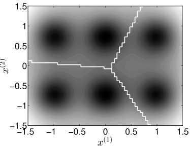
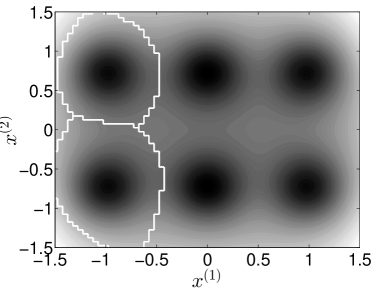
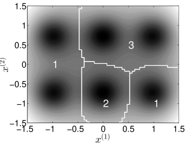
For metastable state decomposition of Model I, we generate 101010 trajectories by 101010 independent simulations with time length 808080, sample interval Δt=0.2Δ𝑡0.2\Delta t=0.2 and initial states 𝐱0subscript𝐱0\mathbf{x}_{0} distributed according to an uniform distribution on [1.5,1.5]2superscript1.51.52\left[-1.5,1.5\right]^{2}. Fig. 3 shows the potential energy and simulation trajectories, where 𝐱t=(xt(1),xt(2))subscript𝐱𝑡superscriptsubscript𝑥𝑡1superscriptsubscript𝑥𝑡2\mathbf{x}_{t}=(x_{t}^{(1)},x_{t}^{(2)}) denotes the system state at time t𝑡t, the potential function V(𝐱)𝑉𝐱V\left(\mathbf{x}\right) is defined by π(𝐱)exp(V(𝐱))proportional-to𝜋𝐱𝑉𝐱\pi\left(\mathbf{x}\right)\propto\exp\left(-V\left(\mathbf{x}\right)\right) and π(𝐱)𝜋𝐱\pi\left(\mathbf{x}\right) is the equilibrium distribution limtp(𝐱t=𝐱)subscript𝑡𝑝subscript𝐱𝑡𝐱\lim_{t\to\infty}p\left(\mathbf{x}_{t}=\mathbf{x}\right). We can observe that Model I has 666 potential wells, and the energy barrier between the “upper” wells (with x(2)>0superscript𝑥20x^{(2)}>0) and the “lower” ones (with x(2)<0superscript𝑥20x^{(2)}<0) can be easily crossed. Therefore, the phase space of Model I can be decomposed into 333 metastable states with each one containing an upper and a lower potential well. Fig. 4 displays the decomposition results of all four methods with κ=3𝜅3\kappa=3 by using the trajectory data shown in Fig. 3b, where the bin number of PCCA+ is set to be 101010. It is obvious that M3C and PCCA+ accurately identify the three metastable states, while the macrostates given by k𝑘k-medoids and MMC do not exhibit strong metastability although the decomposition results of the latter two methods are “reasonable” in the sense of geometric clustering. This shows the limitation of geometric clustering methods in the case that the spatial structure of metastable states does not only depend on the shape of equilibrium state distribution function.

Note that the decomposition result displayed in Fig. 4c might not be the global optima of the MMC problem. It is natural to ask if MMC can correctly find the metastable states by choosing a better initial solution for the local search procedure. In order to answer this question, we solve the MMC problem by the local search algorithm in [43] starting from the decomposition provided by M3C . Fig. 5 shows the corresponding decomposition result, which is very similar to that obtained by M3C and PCCA+. However, the objective function value of this decomposition in the MMC problem is 0.06520.06520.0652, which is larger than the objective function value 0.04960.04960.0496 of the decomposition shown in Fig. 4c. This indicates that MMC prefer the decomposition in Fig. 4c to that in Fig. 5, although the latter one is better for metastability analysis.

Moreover, we also perform the local search algorithm to solve the M3C problem with random initialization, and Fig. 6 plots the optimization result. As observed from the figure, the randomly generated initial solution leads to the algorithm getting stuck in a local optimum. (The optimal objective function values of the M3C problem obtained by the local search with random initialization and the mixed-algorithm proposed in Section 5.3 are 0.15530.15530.1553 and 0.09670.09670.0967 separately.) It shows that the local search algorithm proposed in Section 5.2 is sensitive to initial conditions, and some heuristic method (e.g., the global search algorithm presented in this paper) is needed to provide a satisfactory initial solution.
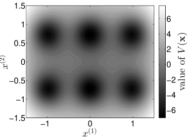
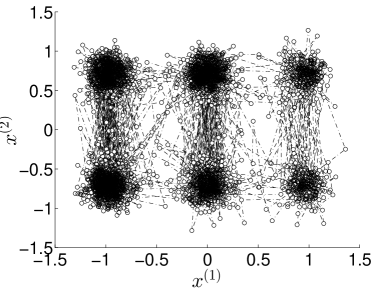
Refer to caption
(a) Potential function
Refer to caption
(b) Trajectory data, where dotted lines represent trajectories of 𝐱tsubscript𝐱𝑡\mathbf{x}_{t} and circles denote data points sampled from trajectories.
Figure 3: Illustration of Model I.
Refer to caption
(a) M3C
Refer to caption
(b) k𝑘k-medoids
Refer to caption
(c) MMC
Refer to caption
(d) PCCA+ (with 10 bins)
Figure 4: Decomposition results of Model I, where white lines represent boundaries between macrostates. The boundaries are computed by the finite element method with mesh size 0.05×0.050.050.050.05\times 0.05.
Refer to caption
Figure 5: Decomposition result of Model I obtained by the local search based MMC with initial solution given by M3C .
Refer to caption
Figure 6: Decomposition result of Model I obtained by the local search based M3C with random initialization.

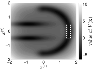
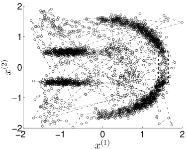
The potential energy of Model II is shown in Fig. 7a. We generate 505050 trajectories in the state space of Model II in order to test the metastable state decomposition methods (see Fig 7b), where the time length of each trajectory is 111, the sample interval is Δt=0.02Δ𝑡0.02\Delta t=0.02 and the initial states are uniformly sampled from [2,2]2superscript222\left[-2,2\right]^{2}. It is easy to see that Model II has three metastable states formed by the three potential wells.

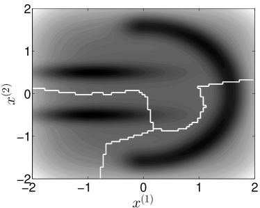
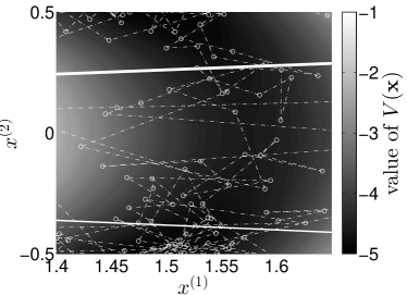
Fig. 8 summarizes the decomposition results with κ=3𝜅3\kappa=3. Figs. 8b and 8c show that k𝑘k-medoids and MMC fail to identify the three metastable states in Model II due to the large difference between the empirical data distribution and the equilibrium distribution. It is interesting to see from Fig. 8d that PCCA+ (with 202020 discrete bins) also gives an undesired decomposition. We now analyze why PCCA+ fails in this example. Note that there is a low energy barrier at the center of the right potential well (see the rectangular region with the dashed line in Fig. 7 and its magnified picture shown in Fig. 9), which can be easily crossed for equilibrium simulations. But the trajectory data used in the above is very far away from the global equilibrium due to short simulation lengths. So only a small number of transitions between discrete bins of PCCA+ are observed around this region, and the PCCA+ assigns these bins to different metastable states. In all the four methods, M3C is the only method that get correct metastable state decomposition by utilizing both the geometric and the dynamical information, and it avoids splitting the right potential well into two metastable states as PCCA+ because such a decomposition leads to a small margin between metastable boundaries.
Refer to caption
(a) Potential function
Refer to caption
(b) Trajectory data, where dotted lines represent trajectories of 𝐱tsubscript𝐱𝑡\mathbf{x}_{t} and circles denote data points sampled from trajectories.
Figure 7: Illustration of Model II, where the rectangular with dashed lines shows the region [1.4,1.65]×[0.5,0.5]1.41.650.50.5[1.4,1.65]\times[-0.5,0.5] of a low energy barrier within the right potential well.
Refer to caption
(a) M3C
Refer to caption
(b) k𝑘k-medoids
Refer to caption
(c) MMC
Refer to caption
(d) PCCA+ (with 20 bins)
Figure 8: Decomposition results of Model II, where white lines represent boundaries between macrostates. The boundaries are computed by the finite element method with mesh size 0.05×0.050.050.050.05\times 0.05.
Refer to caption
Figure 9: PCCA+ decomposition result of Model II in the area [1.4,1.65]×[0.5,0.5]1.41.650.50.5[1.4,1.65]\times[-0.5,0.5], where where dotted lines represent trajectories, circles denote data points sampled from trajectories, solid lines show boundaries of discrete bins obtained by space discretization, and the upper boundary is chosen to be the metastable state boundary by the PCCA+ algorithm.

Finally, we repeat the above numerical experiments of Model I and Model II for 202020 times and utilize the following quantities to evaluate and compare the performance of different decomposition methods quantitatively:

  1. 1.

    Q=k=1κPkk(Δt)𝑄superscriptsubscript𝑘1𝜅subscript𝑃𝑘𝑘Δ𝑡Q=\sum_{k=1}^{\kappa}P_{kk}\left(\Delta t\right), where ΔtΔ𝑡\Delta t denotes the sample interval and

    Pij(τ)subscript𝑃𝑖𝑗𝜏\displaystyle P_{ij}\left(\tau\right) =\displaystyle= limtPr(𝐱t+τmetastable state j|𝐱t\displaystyle\lim_{t\to\infty}\Pr(\mathbf{x}_{t+\tau}\in\text{metastable state }j|\mathbf{x}_{t}\in (28)
    metastable state i)\displaystyle\text{metastable state }i)

    denotes the transition probability between metastable states with lagtime τ𝜏\tau. It is clear that Q𝑄Q can measure the metastability of a system and a decomposition with strongly metastablity will result in a large Q𝑄Q close to κ𝜅\kappa [32].

  2. 2.

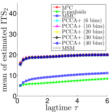
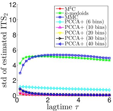
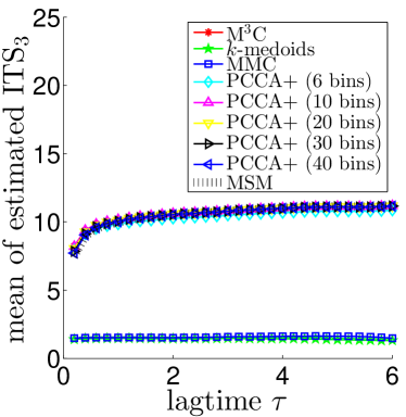
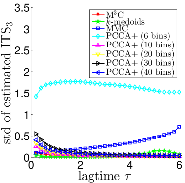
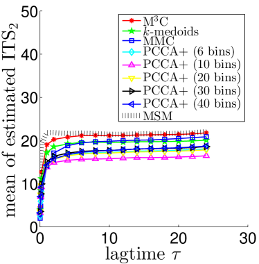
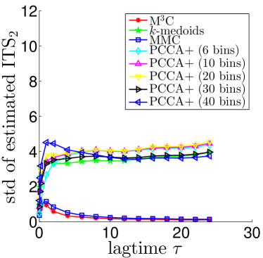
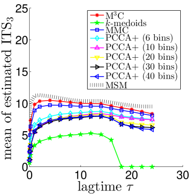
    Implied timescale ITSi(τ)=τ/lnλi(τ)subscriptITS𝑖𝜏𝜏subscript𝜆𝑖𝜏\mathrm{ITS}_{i}\left(\tau\right)=-\tau/\ln\lambda_{i}\left(\tau\right) with i>1𝑖1i>1, where λi(τ)subscript𝜆𝑖𝜏\lambda_{i}\left(\tau\right) denotes the i𝑖i-th largest eigenvalue of transition probability matrix 𝐏(τ)=[Pij(τ)]𝐏𝜏delimited-[]subscript𝑃𝑖𝑗𝜏\mathbf{P}\left(\tau\right)=[P_{ij}\left(\tau\right)]. (The first implied timescale ITSi(τ)subscriptITS𝑖𝜏\mathrm{ITS}_{i}\left(\tau\right)\equiv\infty) It can be proved that the value of ITSi(τ)subscriptITS𝑖𝜏\mathrm{ITS}_{i}\left(\tau\right) is a constant independent of τ𝜏\tau and equal to the dominant relaxation timescales of the original system if the transitions between metastable states are exactly Markovian [16, 12]. Thus, we can check if a Markov chain on metastable states can accurately approximate the system dynamics through comparing implied timescales with different τ𝜏\tau.

Remark 11.

We run a long simulation with time length 104superscript10410^{4} to estimate values of Pij(τ)subscript𝑃𝑖𝑗𝜏P_{ij}\left(\tau\right) for each model. Furthermore, for convenience of comparison, we use the finely discretized Markov state models with 505050 states to estimate the true relaxation timescales of Model I and Model II. The detailed estimation algorithms are given in [5].

Table 3 and Figs. 10 and 11 summarize the values of Q𝑄Q and implied timescales given by different decomposition methods, including the PCCA+ method with different bin numbers. The table and figures also demonstrate the superior performance of M3C. It is worth pointing out that in 999 out of 202020 experiments of Model II, PCCA+ wrongly decomposes the right potential well into two metastable states (with any bin number), whereas M3C gives the “ideal” decomposition in all the 202020 experiments. Moreover, as can be seen from the figures, the implied timescales obtained from M3C converge fast and are very close to the relaxation timescales estimated by finely discretized Markov state models, which implies that the essential dynamical properties of Model I and Model II can be accurately captured by 333-state Markov models using the metastable states identified by M3C.

Table 3: Means and standard deviations of Q𝑄Q values calculated over 202020 independent experiments of Models I and II
k𝑘k-medoids MMC PCCA+(6 bins)PCCA+(6 bins)\begin{array}[]{c}\text{PCCA+}\\ \text{(6 bins)}\end{array} PCCA+(10 bins)PCCA+(10 bins)\begin{array}[]{c}\text{PCCA+}\\ \text{(10 bins)}\end{array} PCCA+(20 bins)PCCA+(20 bins)\begin{array}[]{c}\text{PCCA+}\\ \text{(20 bins)}\end{array} PCCA+(30 bins)PCCA+(30 bins)\begin{array}[]{c}\text{PCCA+}\\ \text{(30 bins)}\end{array} PCCA+(40 bins)PCCA+(40 bins)\begin{array}[]{c}\text{PCCA+}\\ \text{(40 bins)}\end{array} M3C
Model I 2.8138±0.0317plus-or-minus2.81380.03172.8138\pm 0.0317 2.8142±0.0244plus-or-minus2.81420.02442.8142\pm 0.0244 2.9603±0.0170plus-or-minus2.96030.01702.9603\pm 0.0170 2.9637±0.0011plus-or-minus2.96370.00112.9637\pm 0.0011 2.9628±0.0017plus-or-minus2.96280.00172.9628\pm 0.0017 2.9619±0.0027plus-or-minus2.96190.00272.9619\pm 0.0027 2.9613±0.0021plus-or-minus2.96130.00212.9613\pm 0.0021 2.9641±0.0005plus-or-minus2.96410.0005\mathbf{2.9641\pm 0.0005}
Model II 2.9579±0.0031plus-or-minus2.95790.00312.9579\pm 0.0031 2.9832±0.0116plus-or-minus2.98320.01162.9832\pm 0.0116 2.9681±0.0211plus-or-minus2.96810.02112.9681\pm 0.0211 2.9666±0.0161plus-or-minus2.96660.01612.9666\pm 0.0161 2.9676±0.0173plus-or-minus2.96760.01732.9676\pm 0.0173 2.9655±0.0187plus-or-minus2.96550.01872.9655\pm 0.0187 2.9600±0.0285plus-or-minus2.96000.02852.9600\pm 0.0285 2.9882±0.0024plus-or-minus2.98820.0024\mathbf{2.9882\pm 0.0024}
Refer to caption
(a)
Refer to caption
(b)
Refer to caption
(c)
Refer to caption
(d)
Figure 10: Means and standard deviations of estimated implied timescales of Model I obtained by different decomposition methods, where dotted lines indicate estimates of the second and third relaxation timescales of Model I computed by 505050-state Markov state models.
Refer to caption
(a)
Refer to caption
(b)
Refer to caption
(c)
Refer to caption
(d)
Figure 11: Means and standard deviations of estimated implied timescales of Model II obtained by different decomposition methods, where dotted lines indicate estimates of the second and third relaxation timescales of Model II computed by 505050-state Markov state models. (The implied timescale value is set to be zero if the corresponding eigenvalue of the transition probability matrix is zero or negative.)

6.3 Molecular dynamics simulations

We consider in this section the metastable state decomposition problem of molecular dynamics simulation models of alanine dipeptide and deca-alanine. Alanine dipeptide (sequence acetyl-alanine-methylamide) is a small molecule which consists of two alanine amino acid units. The structural and dynamical properties of this molecule have been thoroughly studied, and its conformation space (phase space) can be conveniently described by two backbone dihedral angles φ𝜑\varphi and ψ𝜓\psi (see Fig. 12). Deca-alanine is a small peptide composed of 101010 alanine residues, and its configuration can be described by 181818 backbone dihedral angles. We perform twenty simulations of 200ns200ns200\mathrm{ns} of molecular dynamics of alanine dipeptide with sample interval 20ps20ps20\mathrm{ps} and six 500ns500ns500\mathrm{ns} molecular dynamics simulations of deca-alanine with sample interval 100ps100ps100\mathrm{ps} (The detailed simulation model is given in [56]).
Refer to caption
Figure 12: Illustration of the structure of alanine dipeptide

The metastable state decomposition methods are applied to each simulation trajectory (κ=3𝜅3\kappa=3 for alanine dipeptide and κ=2𝜅2\kappa=2 for deca-alanine), and the corresponding Q𝑄Q values and implied timescales are calculated from all the other trajectories of the same molecule. Moreover, considering the periodicity of angular data, we represent the molecular state as a vector 𝐱𝐱\mathbf{x} consisting of sin/cos of the dihedral angles in experiments.

Fig. 13a shows the potential function of alanine dipeptide in the space of (φ,ψ)𝜑𝜓(\varphi,\psi) and the three metastable states which can be manually identified according to experience, and data points sampled from one simulation trajectory are displayed in Fig. 13b. The decomposition results of the simulation trajectory are plotted in Fig. 14. As can be seen, k𝑘k-medoids and MMC fail to indentify the metastable structure of alanine dipeptide, and the decompositions obtained by PCCA+ and M3C are consistent with the manual decomposition. Table 4 and Fig. 15 summarize Q𝑄Q values and implied timescales given by decomposition results of simulation trajectories of alanine dipeptide. It can be observed that PCCA+ and M3C performs significantly better than the geometric clustering methods k𝑘k-medoids and MMC. M3C achieves the similar average Q𝑄Q values and implied timescales as PCCA+, but the corresponding standard deviations of M3C are lower than that of PCCA+, which shows M3C has more stable performance for this molecular dynamics simulation model.

The decomposition results of deca-alanine are displayed in Table 4 and Fig. 16. The Q𝑄Q values obtained by M3C are significantly smaller than that given by the other methods. In contrast to alanine dipeptide, the kinetics of deca-alanine is much more complicated and it is difficult to accurately estimate the relaxation timescales. In [56], a lower bound 6.5ns6.5ns6.5\mathrm{ns} for the second relaxation timescale is given. Moreover, according to the variational principle [57], the second implied timescale obtained from a metastable state decomposition is always smaller than the true one if there is no statistical noise. So we can conclude from Fig. 16 that M3C gives more accurate estimate of ITS2subscriptITS2\mathrm{ITS}_{2} than the other methods for this molecular dynamics model.
Refer to caption
(a) Potential function estimated from simulation trajectories, where dashed lines represent boundaries between 333 metastable states which are manually identified.
Refer to caption
(b) Data points sampled from a simulation trajectory with sample interval Δt=20psΔ𝑡20ps\Delta t=20\mathrm{ps}.
Figure 13: Illustration of the molecular dynamics simulation of alanine dipetide
Refer to caption
(a) M3C
Refer to caption
(b) k𝑘k-medoids
Refer to caption
(c) MMC
Refer to caption
(d) PCCA+ (with 200200200 bins)
Figure 14: Decomposition results of the simulation model of alanine dipetide, where black lines represent boundaries between macrostates. The boundaries are computed by the finite element method with mesh size 0.05π×0.05π0.05𝜋0.05𝜋0.05\pi\times 0.05\pi.
Table 4: Means and standard deviations of Q𝑄Q values calculated over 101010 independent experiments of alanine dipeptide and 666 independent experiments of deca-alanine
k𝑘k-medoids MMC PCCA+(100 bins)PCCA+(100 bins)\begin{array}[]{c}\text{PCCA+}\\ \text{(100 bins)}\end{array} PCCA+(200 bins)PCCA+(200 bins)\begin{array}[]{c}\text{PCCA+}\\ \text{(200 bins)}\end{array} PCCA+(300 bins)PCCA+(300 bins)\begin{array}[]{c}\text{PCCA+}\\ \text{(300 bins)}\end{array} PCCA+(400 bins)PCCA+(400 bins)\begin{array}[]{c}\text{PCCA+}\\ \text{(400 bins)}\end{array} PCCA+(500 bins)PCCA+(500 bins)\begin{array}[]{c}\text{PCCA+}\\ \text{(500 bins)}\end{array} M3C
alanine dipeptide 1.7655±0.0027plus-or-minus1.76550.00271.7655\pm 0.0027 2.1521±0.5060plus-or-minus2.15210.50602.1521\pm 0.5060 2.7360±0.0077plus-or-minus2.73600.00772.7360\pm 0.0077 2.7381±0.0018plus-or-minus2.73810.00182.7381\pm 0.0018 2.7367±0.0059plus-or-minus2.73670.00592.7367\pm 0.0059 2.7340±0.0037plus-or-minus2.73400.00372.7340\pm 0.0037 2.7328±0.0052plus-or-minus2.73280.00522.7328\pm 0.0052 2.7397±0.0003plus-or-minus2.73970.0003\mathbf{2.7397\pm 0.0003}
deca-alanine 1.8113±0.0502plus-or-minus1.81130.05021.8113\pm 0.0502 1.8819±0.0454plus-or-minus1.88190.04541.8819\pm 0.0454 1.9033±0.0292plus-or-minus1.90330.02921.9033\pm 0.0292 1.8904±0.0402plus-or-minus1.89040.04021.8904\pm 0.0402 1.8894±0.0815plus-or-minus1.88940.08151.8894\pm 0.0815 1.9227±0.0238plus-or-minus1.92270.02381.9227\pm 0.0238 1.8896±0.0764plus-or-minus1.88960.07641.8896\pm 0.0764 1.9592±0.0038plus-or-minus1.95920.0038\mathbf{1.9592\pm 0.0038}
Refer to caption
(a)
Refer to caption
(b)
Refer to caption
(c)
Refer to caption
(d)
Figure 15: Means and standard deviations of estimated implied timescales of alanine dipeptide obtained by different decomposition methods, where dotted lines indicate estimates of the second and third relaxation timescales of alanine dipeptide computed by 500500500-state Markov state models.
Refer to caption
(a) Model I
Refer to caption
(b) Model II
Figure 16: Means and standard deviations of estimated implied timescales of deca-alanine obtained by different decomposition methods.

7 Conclusion

Large margin methods have turned out to be an effective and robust approach for supervised and unsupervised learning problems. In this paper, we apply the large margin principle to the metastable state decomposition problem, and propose a maximum margin metastable clustering (M3C) method to identify metastable states of complex stochastic systems. The key step is to design a large margin metastable constraint (9) by combining the metastability criterion and large margin criterion, where we assign a class label to each transition pair in trajectories instead of a single data point. Then the error of metastable state decomposition can be expressed by the misclassification loss function in large margin learning, and a lot of well developed computational techniques for large margin learning, such as kernel based feature mapping and convex relaxation, can be utilized. Moreover, we present a hybrid optimization algorithm which mixes global search and local search strategies to solve M3C problems with large-scale data sets. In contrast to previous metastable state decomposition methods including geometric clustering methods and kinetic clustering methods, the M3C method can effectively utilize both the geometric information and the dynamical information provided by trajectories without pre-discretization in space, and our experimental analysis reveal that the M3C method yields more accurate and robust decomposition results than traditional geometric and kinetics clustering methods in most cases.

The major drawback of M3C is that the computing burden will be heavy for very large data set, because it need to iteratively solve an SVM-like problem. In the future, we will use some modern SVM techniques such as Pegasos[58] and core vector machine[59] to improve the efficiency of M3C. Moreover, we will investigate how to extend our method to the problem of slow process decomposition of metastable systems [57, 60] by incorporating the distance metric learning technique [61] so that it can not only detect metastable states but also extract dominant dynamical features from simulation and experimental data.

Acknowledgments

This work is supported by the Deutsche Forschungsgemeinschaft (DFG) under grant Number WU 744/1-1, and the author would like to thank Feliks Nüske (FU Berlin) for providing the molecular dynamics simulation data.

Appendix A Proof of equivalence between (9) and (12)

Suppose first that (12) holds. Substituting (k¯,k¯)=(k,yn)¯𝑘¯𝑘𝑘subscript𝑦𝑛(\bar{k},\underaccent{\bar}{k})=(k,y_{n}) and (k¯,k¯)=(yn,k)¯𝑘¯𝑘subscript𝑦𝑛𝑘(\bar{k},\underaccent{\bar}{k})=(y_{n},k) into (12), we can get

(𝐰ynyn𝐰k¯k¯)ϕ(𝐱¯n,𝐱¯n)+(bynynbk¯k¯)+1yn=k¯=k¯=(𝐰yn𝐰k)ϕ(𝐱¯n)+(bynbk)+1yn=k1superscriptsubscript𝐰subscript𝑦𝑛subscript𝑦𝑛superscriptsubscript𝐰¯𝑘¯𝑘bold-italic-ϕsubscript¯𝐱𝑛subscript¯𝐱𝑛subscript𝑏subscript𝑦𝑛subscript𝑦𝑛subscript𝑏¯𝑘¯𝑘subscript1subscript𝑦𝑛¯𝑘¯𝑘superscriptsubscript𝐰subscript𝑦𝑛superscriptsubscript𝐰𝑘bold-italic-ϕsubscript¯𝐱𝑛subscript𝑏subscript𝑦𝑛subscript𝑏𝑘subscript1subscript𝑦𝑛𝑘1\begin{array}[]{l}\left(\mathbf{w}_{y_{n}y_{n}}^{\intercal}-\mathbf{w}_{\bar{k}\underaccent{\bar}{k}}^{\intercal}\right)\bm{\phi}\left(\bar{\mathbf{x}}_{n},\underaccent{\bar}{\mathbf{x}}_{n}\right)+\left(b_{y_{n}y_{n}}-b_{\bar{k}\underaccent{\bar}{k}}\right)+1_{y_{n}=\bar{k}=\underaccent{\bar}{k}}\\ \begin{array}[]{rl}=&\left(\mathbf{w}_{y_{n}}^{\intercal}-\mathbf{w}_{k}^{\intercal}\right)\bm{\phi}\left(\bar{\mathbf{x}}_{n}\right)+\left(b_{y_{n}}-b_{k}\right)+1_{y_{n}=k}\\ \geq&1\end{array}\end{array} (29)

and

(𝐰ynyn𝐰k¯k¯)ϕ(𝐱¯n,𝐱¯n)+(bynynbk¯k¯)+1yn=k¯=k¯=(𝐰yn𝐰k)ϕ(𝐱¯n)+(bynbk)+1yn=k1superscriptsubscript𝐰subscript𝑦𝑛subscript𝑦𝑛superscriptsubscript𝐰¯𝑘¯𝑘bold-italic-ϕsubscript¯𝐱𝑛subscript¯𝐱𝑛subscript𝑏subscript𝑦𝑛subscript𝑦𝑛subscript𝑏¯𝑘¯𝑘subscript1subscript𝑦𝑛¯𝑘¯𝑘superscriptsubscript𝐰subscript𝑦𝑛superscriptsubscript𝐰𝑘bold-italic-ϕsubscript¯𝐱𝑛subscript𝑏subscript𝑦𝑛subscript𝑏𝑘subscript1subscript𝑦𝑛𝑘1\begin{array}[]{l}\left(\mathbf{w}_{y_{n}y_{n}}^{\intercal}-\mathbf{w}_{\bar{k}\underaccent{\bar}{k}}^{\intercal}\right)\bm{\phi}\left(\bar{\mathbf{x}}_{n},\underaccent{\bar}{\mathbf{x}}_{n}\right)+\left(b_{y_{n}y_{n}}-b_{\bar{k}\underaccent{\bar}{k}}\right)+1_{y_{n}=\bar{k}=\underaccent{\bar}{k}}\\ \begin{array}[]{rl}=&\left(\mathbf{w}_{y_{n}}^{\intercal}-\mathbf{w}_{k}^{\intercal}\right)\bm{\phi}\left(\underaccent{\bar}{\mathbf{x}}_{n}\right)+\left(b_{y_{n}}-b_{k}\right)+1_{y_{n}=k}\\ \geq&1\end{array}\end{array} (30)

So (12) is a sufficient condition for (9).

We now show the necessity of (12) for (9). Substituting k=k¯𝑘¯𝑘k=\bar{k} and k=k¯𝑘¯𝑘k=\underaccent{\bar}{k} into the two inequalities in (9), respectively, yields

(𝐰ynyn𝐰k¯k¯)ϕ(𝐱¯n,𝐱¯n)+(bynynbk¯k¯)+(1yn=k¯+1yn=k¯1)1superscriptsubscript𝐰subscript𝑦𝑛subscript𝑦𝑛superscriptsubscript𝐰¯𝑘¯𝑘bold-italic-ϕsubscript¯𝐱𝑛subscript¯𝐱𝑛subscript𝑏subscript𝑦𝑛subscript𝑦𝑛subscript𝑏¯𝑘¯𝑘subscript1subscript𝑦𝑛¯𝑘subscript1subscript𝑦𝑛¯𝑘11\left(\mathbf{w}_{y_{n}y_{n}}^{\intercal}-\mathbf{w}_{\bar{k}\underaccent{\bar}{k}}^{\intercal}\right)\bm{\phi}\left(\bar{\mathbf{x}}_{n},\underaccent{\bar}{\mathbf{x}}_{n}\right)+\left(b_{y_{n}y_{n}}-b_{\bar{k}\underaccent{\bar}{k}}\right)+\left(1_{y_{n}=\bar{k}}+1_{y_{n}=\underaccent{\bar}{k}}-1\right)\geq 1 (31)

Note that

1yn=k¯+1yn=k¯1={1,yn=k¯=k¯0,yn{k¯,k¯},k¯k¯1,otherwisesubscript1subscript𝑦𝑛¯𝑘subscript1subscript𝑦𝑛¯𝑘1cases1subscript𝑦𝑛¯𝑘¯𝑘0formulae-sequencesubscript𝑦𝑛¯𝑘¯𝑘¯𝑘¯𝑘1otherwise1_{y_{n}=\bar{k}}+1_{y_{n}=\underaccent{\bar}{k}}-1=\left\{\begin{array}[]{ll}1,&y_{n}=\bar{k}=\underaccent{\bar}{k}\\ 0,&y_{n}\in\{\bar{k},\underaccent{\bar}{k}\},\bar{k}\neq\underaccent{\bar}{k}\\ -1,&\mathrm{otherwise}\end{array}\right. (32)

and

1yn=k¯=k¯={1,yn=k¯=k¯0,otherwisesubscript1subscript𝑦𝑛¯𝑘¯𝑘cases1subscript𝑦𝑛¯𝑘¯𝑘0otherwise1_{y_{n}=\bar{k}=\underaccent{\bar}{k}}=\left\{\begin{array}[]{ll}1,&y_{n}=\bar{k}=\underaccent{\bar}{k}\\ 0,&\mathrm{otherwise}\end{array}\right. (33)

Therefore,

(𝐰ynyn𝐰k¯k¯)ϕ(𝐱¯n,𝐱¯n)+(bynynbk¯k¯)+1yn=k¯=k¯(𝐰ynyn𝐰k¯k¯)ϕ(𝐱¯n,𝐱¯n)+(bynynbk¯k¯)+(1yn=k¯+1yn=k¯1)1superscriptsubscript𝐰subscript𝑦𝑛subscript𝑦𝑛superscriptsubscript𝐰¯𝑘¯𝑘bold-italic-ϕsubscript¯𝐱𝑛subscript¯𝐱𝑛subscript𝑏subscript𝑦𝑛subscript𝑦𝑛subscript𝑏¯𝑘¯𝑘subscript1subscript𝑦𝑛¯𝑘¯𝑘superscriptsubscript𝐰subscript𝑦𝑛subscript𝑦𝑛superscriptsubscript𝐰¯𝑘¯𝑘bold-italic-ϕsubscript¯𝐱𝑛subscript¯𝐱𝑛subscript𝑏subscript𝑦𝑛subscript𝑦𝑛subscript𝑏¯𝑘¯𝑘subscript1subscript𝑦𝑛¯𝑘subscript1subscript𝑦𝑛¯𝑘11\begin{array}[]{l}\left(\mathbf{w}_{y_{n}y_{n}}^{\intercal}-\mathbf{w}_{\bar{k}\underaccent{\bar}{k}}^{\intercal}\right)\bm{\phi}\left(\bar{\mathbf{x}}_{n},\underaccent{\bar}{\mathbf{x}}_{n}\right)+\left(b_{y_{n}y_{n}}-b_{\bar{k}\underaccent{\bar}{k}}\right)+1_{y_{n}=\bar{k}=\underaccent{\bar}{k}}\\ \begin{array}[]{rl}\geq&\left(\mathbf{w}_{y_{n}y_{n}}^{\intercal}-\mathbf{w}_{\bar{k}\underaccent{\bar}{k}}^{\intercal}\right)\bm{\phi}\left(\bar{\mathbf{x}}_{n},\underaccent{\bar}{\mathbf{x}}_{n}\right)+\left(b_{y_{n}y_{n}}-b_{\bar{k}\underaccent{\bar}{k}}\right)+\left(1_{y_{n}=\bar{k}}+1_{y_{n}=\underaccent{\bar}{k}}-1\right)\\ \geq&1\end{array}\end{array} (34)

From the above, we can conclude that (12) is equivalent to (9).

Appendix B Proof of Theorem 5

Let us start with the case that all labels 𝐲csuperscript𝐲𝑐\mathbf{y}^{c} in (14) are given. In this case, the coarse-grained M3C problem (14) is reduced to a simple quadratic programming problem:

min𝐖,𝝃c12β𝐖2+𝐜𝝃cs.t.n=1,,Nc,k¯,k¯=1,,κ,(𝐰yncync𝐰k¯k¯)ϕ(𝐱¯nc,𝐱¯n)+1ync=k¯=k¯1ξnc,subscript𝐖superscript𝝃𝑐12𝛽superscriptnorm𝐖2superscript𝐜superscript𝝃𝑐formulae-sequencestformulae-sequencefor-all𝑛1superscript𝑁𝑐for-all¯𝑘¯𝑘1𝜅missing-subexpressionsuperscriptsubscript𝐰superscriptsubscript𝑦𝑛𝑐superscriptsubscript𝑦𝑛𝑐superscriptsubscript𝐰¯𝑘¯𝑘bold-italic-ϕsuperscriptsubscript¯𝐱𝑛𝑐subscript¯𝐱𝑛subscript1superscriptsubscript𝑦𝑛𝑐¯𝑘¯𝑘1superscriptsubscript𝜉𝑛𝑐\begin{array}[]{cl}\min\limits_{\mathbf{W},\bm{\xi}^{c}}&\frac{1}{2}\beta\left\|\mathbf{W}\right\|^{2}+\mathbf{c}^{\intercal}\bm{\xi}^{c}\\ \mathrm{s.t.}&\forall n=1,\ldots,N^{c},\quad\forall\bar{k},\underaccent{\bar}{k}=1,\ldots,\kappa,\\ &\left(\mathbf{w}_{y_{n}^{c}y_{n}^{c}}^{\intercal}-\mathbf{w}_{\bar{k}\underaccent{\bar}{k}}^{\intercal}\right)\bm{\phi}\left(\bar{\mathbf{x}}_{n}^{c},\underaccent{\bar}{\mathbf{x}}_{n}\right)+1_{y_{n}^{c}=\bar{k}=\underaccent{\bar}{k}}\geq 1-\xi_{n}^{c},\end{array} (35)

For the sake of convenience, here we let 𝐞ksubscript𝐞𝑘\mathbf{e}_{k} denote a κ𝜅\kappa dimensional vector with only the k𝑘k-th element being 111 and others 00, and define a matrix 𝐁2κ×κ2𝐁superscript2𝜅superscript𝜅2\mathbf{B}\in\mathbb{R}^{2\kappa\times\kappa^{2}} as

𝐁=[𝐁¯𝐁¯]=[𝐞1𝐞2𝐞κ𝐞1𝐞1𝐞κ𝐞1𝐞2𝐞κ𝐞2𝐞3𝐞κ1]𝐁delimited-[]¯𝐁¯𝐁delimited-[]subscript𝐞1subscript𝐞2subscript𝐞𝜅subscript𝐞1subscript𝐞1subscript𝐞𝜅subscript𝐞1subscript𝐞2subscript𝐞𝜅subscript𝐞2subscript𝐞3subscript𝐞𝜅1\mathbf{B}=\left[\begin{array}[]{c}\bar{\mathbf{B}}\\ \underaccent{\bar}{\mathbf{B}}\end{array}\right]=\left[\begin{array}[]{cccccccc}\mathbf{e}_{1}&\mathbf{e}_{2}&\cdots&\mathbf{e}_{\kappa}&\mathbf{e}_{1}&\mathbf{e}_{1}&\cdots&\mathbf{e}_{\kappa}\\ \mathbf{e}_{1}&\mathbf{e}_{2}&\cdots&\mathbf{e}_{\kappa}&\mathbf{e}_{2}&\mathbf{e}_{3}&\cdots&\mathbf{e}_{\kappa-1}\end{array}\right] (36)

i.e., each column of 𝐁𝐁\mathbf{B} is an element of {(𝐞i,𝐞j)|i,j[1,κ]}conditional-setsuperscriptsuperscriptsubscript𝐞𝑖superscriptsubscript𝐞𝑗𝑖𝑗1𝜅\{(\mathbf{e}_{i}^{\intercal},\mathbf{e}_{j}^{\intercal})^{\intercal}|i,j\in[1,\kappa]\} and the first κ𝜅\kappa columns of 𝐁𝐁\mathbf{B} is equal to [𝐈𝐈]superscriptdelimited-[]𝐈𝐈\left[\begin{array}[]{cc}\mathbf{I}&\mathbf{I}\end{array}\right]^{\intercal}, where 𝐁¯,𝐁¯κ×κ2¯𝐁¯𝐁superscript𝜅superscript𝜅2\bar{\mathbf{B}},\underaccent{\bar}{\mathbf{B}}\in\mathbb{R}^{\kappa\times\kappa^{2}} are two submatrices consisting of the first κ𝜅\kappa and the last κ𝜅\kappa rows of 𝐁𝐁\mathbf{B}.

By introducing a dual variable 𝚲Nc×κ2𝚲superscriptsuperscript𝑁𝑐superscript𝜅2\bm{\Lambda}\in\mathbb{R}^{N^{c}\times\kappa^{2}} and using (15) and (36), the Lagrangian of (35) can be written as

\displaystyle\mathcal{L} =\displaystyle= 12β𝐖2+𝐜𝝃ctr(𝐃diag(𝚲𝟏)(𝐗¯+𝐗¯)𝐖)12𝛽superscriptnorm𝐖2superscript𝐜superscript𝝃𝑐trsuperscript𝐃diag𝚲1¯𝐗¯𝐗superscript𝐖\displaystyle\frac{1}{2}\beta\left\|\mathbf{W}\right\|^{2}+\mathbf{c}^{\intercal}\bm{\xi}^{c}-\mathrm{tr}\left(\mathbf{D}^{\intercal}\mathrm{diag}\left(\bm{\Lambda}\mathbf{1}\right)\left(\bar{\mathbf{X}}+\underaccent{\bar}{\mathbf{X}}\right)\mathbf{W}^{\intercal}\right) (39)
tr([𝚲𝐃𝟎𝟎])+tr(𝚲(𝐗¯𝐖𝐁¯+𝐗¯𝐖𝐁¯))trdelimited-[]superscript𝚲𝐃superscript00trsuperscript𝚲¯𝐗superscript𝐖¯𝐁¯𝐗superscript𝐖¯𝐁\displaystyle-\mathrm{tr}\left(\left[\begin{array}[]{cc}\bm{\Lambda}^{\intercal}\mathbf{D}&\mathbf{0}\mathbf{0}^{\intercal}\end{array}\right]\right)+\mathrm{tr}\left(\bm{\Lambda}^{\intercal}\left(\bar{\mathbf{X}}\mathbf{W}^{\intercal}\bar{\mathbf{B}}+\underaccent{\bar}{\mathbf{X}}\mathbf{W}^{\intercal}\underaccent{\bar}{\mathbf{B}}\right)\right)
+(𝟏𝝃c)𝚲𝟏superscript1superscript𝝃𝑐𝚲1\displaystyle+\left(\mathbf{1}-\bm{\xi}^{c}\right)^{\intercal}\bm{\Lambda}\mathbf{1}

where 𝐗¯=(ϕ(𝐱¯1c),,ϕ(𝐱¯Ncc))Nc×d¯𝐗superscriptbold-italic-ϕsuperscriptsubscript¯𝐱1𝑐bold-italic-ϕsuperscriptsubscript¯𝐱superscript𝑁𝑐𝑐superscriptsuperscript𝑁𝑐𝑑\bar{\mathbf{X}}=\left(\bm{\phi}(\bar{\mathbf{x}}_{1}^{c}),\ldots,\bm{\phi}(\bar{\mathbf{x}}_{N^{c}}^{c})\right)^{\intercal}\in\mathbb{R}^{N^{c}\times d} and 𝐗¯=(ϕ(𝐱¯1c),,ϕ(𝐱¯Ncc))Nc×d¯𝐗superscriptbold-italic-ϕsuperscriptsubscript¯𝐱1𝑐bold-italic-ϕsuperscriptsubscript¯𝐱superscript𝑁𝑐𝑐superscriptsuperscript𝑁𝑐𝑑\underaccent{\bar}{\mathbf{X}}=\left(\bm{\phi}(\underaccent{\bar}{\mathbf{x}}_{1}^{c}),\ldots,\bm{\phi}(\underaccent{\bar}{\mathbf{x}}_{N^{c}}^{c})\right)^{\intercal}\in\mathbb{R}^{N^{c}\times d}. Setting the derivatives of the Lagrangian (39) with respect to 𝐖𝐖\mathbf{W} and 𝝃csuperscript𝝃𝑐\bm{\xi}^{c} to zero, and adding the constraint 𝚲0𝚲0\bm{\Lambda}\geq 0, we obtain the following dual problem of (35):

max𝚲12βtr([𝐁¯𝚲𝐁¯𝚲]𝐊[𝐁¯𝚲𝐁¯𝚲])+1βtr(𝐃𝐂[𝐈𝐈]𝐊[𝐁¯𝚲𝐁¯𝚲])tr([𝚲𝐃𝟎𝟎])12βtr(𝐌𝐂𝐊s𝐂)+𝟏𝐜s.t.𝚲𝟏=𝟏,𝚲0.subscript𝚲12𝛽trdelimited-[]¯𝐁superscript𝚲¯𝐁superscript𝚲𝐊superscriptdelimited-[]¯𝐁superscript𝚲¯𝐁superscript𝚲missing-subexpression1𝛽trsuperscript𝐃𝐂delimited-[]𝐈𝐈𝐊superscriptdelimited-[]¯𝐁superscript𝚲¯𝐁superscript𝚲missing-subexpressiontrdelimited-[]superscript𝚲𝐃superscript0012𝛽trsuperscript𝐌𝐂𝐊𝑠𝐂superscript1𝐜formulae-sequencest𝚲11missing-subexpression𝚲0\begin{array}[]{cl}\max\limits_{\bm{\Lambda}}&-\frac{1}{2\beta}\mathrm{tr}\left(\left[\begin{array}[]{cc}\bar{\mathbf{B}}\bm{\Lambda}^{\intercal}&\underaccent{\bar}{\mathbf{B}}\bm{\Lambda}^{\intercal}\end{array}\right]\mathbf{K}\left[\begin{array}[]{cc}\bar{\mathbf{B}}\bm{\Lambda}^{\intercal}&\underaccent{\bar}{\mathbf{B}}\bm{\Lambda}^{\intercal}\end{array}\right]^{\intercal}\right)\\ &+\frac{1}{\beta}\mathrm{tr}\left(\mathbf{D}^{\intercal}\mathbf{C}\left[\begin{array}[]{cc}\mathbf{I}&\mathbf{I}\end{array}\right]\mathbf{K}\left[\begin{array}[]{cc}\bar{\mathbf{B}}\bm{\Lambda}^{\intercal}&\underaccent{\bar}{\mathbf{B}}\bm{\Lambda}^{\intercal}\end{array}\right]^{\intercal}\right)\\ &-\mathrm{tr}\left(\left[\begin{array}[]{cc}\bm{\Lambda}^{\intercal}\mathbf{D}&\mathbf{0}\mathbf{0}^{\intercal}\end{array}\right]\right)-\frac{1}{2\beta}\mathrm{tr}\left(\mathbf{M}\mathbf{C}\mathbf{K}^{s}\mathbf{C}\right)+\mathbf{1}^{\intercal}\mathbf{c}\\ \mathrm{s.t.}&\bm{\Lambda}\mathbf{1}=\mathbf{1},\\ &\bm{\Lambda}\geq 0.\end{array} (40)

where

𝐊=[𝐊(1,1)𝐊(1,2)𝐊(2,1)𝐊(2,2)]𝐊delimited-[]superscript𝐊11superscript𝐊12superscript𝐊21superscript𝐊22\mathbf{K}=\left[\begin{array}[]{cc}\mathbf{K}^{(1,1)}&\mathbf{K}^{(1,2)}\\ \mathbf{K}^{(2,1)}&\mathbf{K}^{(2,2)}\end{array}\right] (41)
𝐊s=𝐊(1,1)+𝐊(1,2)+𝐊(2,1)+𝐊(2,2)superscript𝐊𝑠superscript𝐊11superscript𝐊12superscript𝐊21superscript𝐊22\mathbf{K}^{s}=\mathbf{K}^{(1,1)}+\mathbf{K}^{(1,2)}+\mathbf{K}^{(2,1)}+\mathbf{K}^{(2,2)} (42)

and

𝐊(1,1)=𝐗¯𝐗¯,𝐊(1,2)=𝐗¯𝐗¯,𝐊(1,1)=𝐗¯𝐗¯,𝐊(1,2)=𝐗¯𝐗¯formulae-sequencesuperscript𝐊11superscript¯𝐗¯𝐗formulae-sequencesuperscript𝐊12superscript¯𝐗¯𝐗formulae-sequencesuperscript𝐊11superscript¯𝐗¯𝐗superscript𝐊12superscript¯𝐗¯𝐗\mathbf{K}^{(1,1)}=\bar{\mathbf{X}}^{\intercal}\bar{\mathbf{X}},\mathbf{K}^{(1,2)}=\bar{\mathbf{X}}^{\intercal}\underaccent{\bar}{\mathbf{X}},\mathbf{K}^{(1,1)}=\underaccent{\bar}{\mathbf{X}}^{\intercal}\bar{\mathbf{X}},\mathbf{K}^{(1,2)}=\underaccent{\bar}{\mathbf{X}}^{\intercal}\underaccent{\bar}{\mathbf{X}} (43)

Putting (40) into the form of a standard quadratic programming problem, we have

max𝚲12βvec(𝚲)𝐏vec(𝚲)+𝐪vec(𝚲)12βtr(𝐌𝐂𝐊s𝐂)+𝟏𝐜s.t.(𝟏𝐈)vec(𝚲)=𝟏,vec(𝚲)0.subscript𝚲12𝛽vecsuperscript𝚲𝐏vec𝚲superscript𝐪vec𝚲12𝛽trsuperscript𝐌𝐂𝐊𝑠𝐂superscript1𝐜formulae-sequencesttensor-productsuperscript1𝐈vec𝚲1missing-subexpressionvec𝚲0\begin{array}[]{cl}\max\limits_{\bm{\Lambda}}&-\frac{1}{2\beta}\mathrm{vec}\left(\bm{\Lambda}\right)^{\intercal}\mathbf{P}\mathrm{vec}\left(\bm{\Lambda}\right)+\mathbf{q}^{\intercal}\mathrm{vec}\left(\bm{\Lambda}\right)-\frac{1}{2\beta}\mathrm{tr}\left(\mathbf{M}\mathbf{C}\mathbf{K}^{s}\mathbf{C}\right)+\mathbf{1}^{\intercal}\mathbf{c}\\ \mathrm{s.t.}&\left(\mathbf{1}^{\intercal}\otimes\mathbf{I}\right)\mathrm{vec}\left(\bm{\Lambda}\right)=\mathbf{1},\\ &\mathrm{vec}\left(\bm{\Lambda}\right)\geq 0.\end{array} (44)

where

𝐏𝐏\displaystyle\mathbf{P} =\displaystyle= (𝐁¯𝐁¯)𝐊(1,1)+(𝐁¯𝐁¯)𝐊(1,2)tensor-productsuperscript¯𝐁¯𝐁superscript𝐊11tensor-productsuperscript¯𝐁¯𝐁superscript𝐊12\displaystyle\left(\bar{\mathbf{B}}^{\intercal}\bar{\mathbf{B}}\right)\otimes\mathbf{K}^{(1,1)}+\left(\bar{\mathbf{B}}^{\intercal}\underaccent{\bar}{\mathbf{B}}\right)\otimes\mathbf{K}^{(1,2)} (45)
+(𝐁¯𝐁¯)𝐊(2,1)+(𝐁¯𝐁¯)𝐊(2,2)tensor-productsuperscript¯𝐁¯𝐁superscript𝐊21tensor-productsuperscript¯𝐁¯𝐁superscript𝐊22\displaystyle+\left(\underaccent{\bar}{\mathbf{B}}^{\intercal}\bar{\mathbf{B}}\right)\otimes\mathbf{K}^{(2,1)}+\left(\underaccent{\bar}{\mathbf{B}}^{\intercal}\underaccent{\bar}{\mathbf{B}}\right)\otimes\mathbf{K}^{(2,2)}

and

𝐪𝐪\displaystyle\mathbf{q} =\displaystyle= vec(1β(𝐊(1,1)+𝐊(2,1))𝐂𝐃𝐁¯\displaystyle\mathrm{vec}\bigg{(}\frac{1}{\beta}\left(\mathbf{K}^{(1,1)}+\mathbf{K}^{(2,1)}\right)^{\intercal}\mathbf{C}^{\intercal}\mathbf{D}\bar{\mathbf{B}} (47)
+1β(𝐊(1,2)+𝐊(2,2))𝐂𝐃𝐁¯[𝐃𝟎𝟎])\displaystyle+\frac{1}{\beta}\left(\mathbf{K}^{(1,2)}+\mathbf{K}^{(2,2)}\right)^{\intercal}\mathbf{C}^{\intercal}\mathbf{D}\underaccent{\bar}{\mathbf{B}}-\left[\begin{array}[]{cc}\mathbf{D}&\mathbf{0}\mathbf{0}^{\intercal}\end{array}\right]\bigg{)}

(The definition of vec()vec\mathrm{vec}\left(\cdot\right) is given in the list of notation.) According to Lemma 12 and the strong duality theorem [62], we can conclude that (35) has the same minimum with the following optimization problem:

min𝜶,𝐯,𝜽12𝜽𝜽𝐜𝜶12βtr(𝐌𝐂𝐊s𝐂)+𝟏𝐜s.t.𝐪+(𝟏𝐈)𝜶+𝐯+𝐑𝜽=0,𝐯0.subscript𝜶𝐯𝜽12superscript𝜽𝜽superscript𝐜𝜶12𝛽trsuperscript𝐌𝐂𝐊𝑠𝐂superscript1𝐜formulae-sequencest𝐪tensor-product1𝐈𝜶𝐯𝐑𝜽0missing-subexpression𝐯0\begin{array}[]{cl}\min\limits_{\bm{\alpha},\mathbf{v},\bm{\theta}}&\frac{1}{2}\bm{\theta}^{\intercal}\bm{\theta}-\mathbf{c}^{\intercal}\bm{\alpha}-\frac{1}{2\beta}\mathrm{tr}\left(\mathbf{M}\mathbf{C}\mathbf{K}^{s}\mathbf{C}\right)+\mathbf{1}^{\intercal}\mathbf{c}\\ \mathrm{s.t.}&\mathbf{q}+\left(\mathbf{1}\otimes\mathbf{I}\right)\bm{\alpha}+\mathbf{v}+\mathbf{R}\bm{\theta}=0,\\ &\mathbf{v}\geq 0.\end{array} (48)

where 𝐑𝐑\mathbf{R} is a full column rank matrix satisfying

1β𝐏=𝐑𝐑1𝛽𝐏superscript𝐑𝐑\frac{1}{\beta}\mathbf{P}=\mathbf{R}\mathbf{R}^{\intercal} (49)

(Note that 𝐑𝐑\mathbf{R} may not be a square matrix if 𝐏𝐏\mathbf{P} is not full rank.)

Combining the equivalence between (35) and (48) and the proposition mentioned in Remark 6, the theorem is proved.

Lemma 12.

For a quadratic programming problem defined by

min𝐱12𝐱𝐀𝐱+𝐛𝐱s.t.𝐄𝐱=𝐜,𝐱0.subscript𝐱12superscript𝐱𝐀𝐱superscript𝐛𝐱formulae-sequencest𝐄𝐱𝐜missing-subexpression𝐱0\begin{array}[]{cl}\min\limits_{\mathbf{x}}&\frac{1}{2}\mathbf{x}^{\intercal}\mathbf{A}\mathbf{x}+\mathbf{b}^{\intercal}\mathbf{x}\\ \mathrm{s.t.}&\mathbf{E}\mathbf{x}=\mathbf{c},\\ &\mathbf{x}\geq 0.\end{array} (50)

if 𝐀𝐀\mathbf{A} can be decomposed as 𝐀=𝐑𝐑𝐀superscript𝐑𝐑\mathbf{A}=\mathbf{R}\mathbf{R}^{\intercal} with 𝐑𝐑\mathbf{R} being full column rank and there is an optimal solution to (50), then the minimum of (50) is equal to the maximum of the following problem:

max𝜶,𝐯,𝜽12𝜽𝜽+𝐜𝜶s.t.𝐛𝜶𝐄𝐯=𝜽𝐑,𝐯0.subscript𝜶𝐯𝜽12superscript𝜽𝜽superscript𝐜𝜶formulae-sequencestsuperscript𝐛superscript𝜶𝐄superscript𝐯superscript𝜽superscript𝐑missing-subexpression𝐯0\begin{array}[]{cl}\max\limits_{\bm{\alpha},\mathbf{v},\bm{\theta}}&-\frac{1}{2}\bm{\theta}^{\intercal}\bm{\theta}+\mathbf{c}^{\intercal}\bm{\alpha}\\ \mathrm{s.t.}&\mathbf{b}^{\intercal}-\bm{\alpha}^{\intercal}\mathbf{E}-\mathbf{v}^{\intercal}=\bm{\theta}^{\intercal}\mathbf{R}^{\intercal},\\ &\mathbf{v}\geq 0.\end{array} (51)
Proof.

The Lagrangian of (50) is

(𝐱,𝜶,𝐯)=12𝐱𝐀𝐱+(𝐛𝜶𝐄𝐯)𝐱+𝐜𝜶𝐱𝜶𝐯12superscript𝐱𝐀𝐱superscript𝐛superscript𝜶𝐄superscript𝐯𝐱superscript𝐜𝜶\mathcal{L}\left(\mathbf{x},\bm{\alpha},\mathbf{v}\right)=\frac{1}{2}\mathbf{x}^{\intercal}\mathbf{A}\mathbf{x}+\left(\mathbf{b}^{\intercal}-\bm{\alpha}^{\intercal}\mathbf{E}-\mathbf{v}^{\intercal}\right)\mathbf{x}+\mathbf{c}^{\intercal}\bm{\alpha} (52)

Then the dual problem of (50) can be written as

max𝜶,𝐯g(𝜶,𝐯)s.t.𝐯0.subscript𝜶𝐯𝑔𝜶𝐯formulae-sequencest𝐯0\begin{array}[]{cl}\max\limits_{\bm{\alpha},\mathbf{v}}&g\left(\bm{\alpha},\mathbf{v}\right)\\ \mathrm{s.t.}&\mathbf{v}\geq 0.\end{array} (53)

with

g(𝜶,𝐯)=inf𝐱(𝐱,𝜶,𝐯)𝑔𝜶𝐯subscriptinfimum𝐱𝐱𝜶𝐯g\left(\bm{\alpha},\mathbf{v}\right)=\inf_{\mathbf{x}}\mathcal{L}\left(\mathbf{x},\bm{\alpha},\mathbf{v}\right) (54)

We now analyze the value of g(𝜶,𝐯)𝑔𝜶𝐯g\left(\bm{\alpha},\mathbf{v}\right) in different cases.

Case (i)

There is a 𝜽𝜽\bm{\theta} such that

𝐛𝜶𝐄𝐯=𝜽𝐑superscript𝐛superscript𝜶𝐄superscript𝐯superscript𝜽superscript𝐑\mathbf{b}^{\intercal}-\bm{\alpha}^{\intercal}\mathbf{E}-\mathbf{v}^{\intercal}=\bm{\theta}^{\intercal}\mathbf{R}^{\intercal} (55)

We have (𝐱,𝜶,𝐯)=12(𝐑𝐱)(𝐑𝐱)+𝜽(𝐑𝐱)+𝐜𝜶𝐱𝜶𝐯12superscriptsuperscript𝐑𝐱superscript𝐑𝐱superscript𝜽superscript𝐑𝐱superscript𝐜𝜶\mathcal{L}\left(\mathbf{x},\bm{\alpha},\mathbf{v}\right)=\frac{1}{2}\left(\mathbf{R}^{\intercal}\mathbf{x}\right)^{\intercal}\left(\mathbf{R}^{\intercal}\mathbf{x}\right)+\bm{\theta}^{\intercal}\left(\mathbf{R}^{\intercal}\mathbf{x}\right)+\mathbf{c}^{\intercal}\bm{\alpha} and g(𝜶,𝐯)=12𝜽𝜽+𝐜𝜶𝑔𝜶𝐯12superscript𝜽𝜽superscript𝐜𝜶g\left(\bm{\alpha},\mathbf{v}\right)=-\frac{1}{2}\bm{\theta}^{\intercal}\bm{\theta}+\mathbf{c}^{\intercal}\bm{\alpha}.

Case (ii)

There is no 𝜽𝜽\bm{\theta} satisfying (55). It is easy to see that we can find an 𝐱𝐱\mathbf{x} such that 𝐑𝐱=0superscript𝐑𝐱0\mathbf{R}^{\intercal}\mathbf{x}=0 and (𝐛𝜶𝐄𝐯)𝐱0superscript𝐛superscript𝜶𝐄superscript𝐯𝐱0\left(\mathbf{b}^{\intercal}-\bm{\alpha}^{\intercal}\mathbf{E}-\mathbf{v}^{\intercal}\right)\mathbf{x}\neq 0. Then g(𝜶,𝐯)=𝑔𝜶𝐯g\left(\bm{\alpha},\mathbf{v}\right)=-\infty.

Combining the above results yields the conclusion of the lemma.

Appendix C Optimization procedure for MMC

The optimization algorithm for solving MMC problems in our experiments is described by Algorithm 2. It can be seen that this algorithm also combines global search and local search techniques through coarse graining like the algorithm for M3C proposed in this paper.

1:  generate a coarse-grained set Scsuperscript𝑆𝑐S^{c} with cardinality Ncsuperscript𝑁𝑐N^{c} and normalized weights 𝐜=(c1,,cNc)𝐜superscriptsubscript𝑐1subscript𝑐superscript𝑁𝑐\mathbf{c}=(c_{1},\ldots,c_{N^{c}})^{\intercal} from 𝒮𝒮\mathcal{S} by the k𝑘k-medoids algorithm
2:  solve the MMC problem on Scsuperscript𝑆𝑐S^{c} by the SDP relaxation algorithm [40] to get class labels 𝐲c=(y1c,,yNcc)superscript𝐲𝑐superscriptsubscript𝑦1𝑐superscriptsubscript𝑦superscript𝑁𝑐𝑐\mathbf{y}^{c}=(y_{1}^{c},\ldots,y_{N^{c}}^{c}) of 𝒮csuperscript𝒮𝑐\mathcal{S}^{c}
3:  calculate class labels 𝐲(0)=(y1,,y|𝒮|)superscript𝐲0subscript𝑦1subscript𝑦𝒮\mathbf{y}^{(0)}=(y_{1},\ldots,y_{\left|\mathcal{S}\right|}) of data points in 𝒮𝒮\mathcal{S} from 𝐲csuperscript𝐲𝑐\mathbf{y}^{c}
4:  solve the MMC problem on 𝒮𝒮\mathcal{S} by the local search algorithm proposed in [43] starting from 𝐲=𝐲(0)𝐲superscript𝐲0\mathbf{y}=\mathbf{y}^{(0)}.
Algorithm 2 Optimization procedure for MMC

Appendix D Implementation procedure of PCCA+

In this paper, we perform the PCCA+ clustering as shown in Algorithm 3.

1:  partition all the data into Ncsuperscript𝑁𝑐N^{c} bins 𝐱1c,,𝐱Nccsuperscriptsubscript𝐱1𝑐superscriptsubscript𝐱superscript𝑁𝑐𝑐\mathbf{x}_{1}^{c},\ldots,\mathbf{x}_{N^{c}}^{c} by the k𝑘k-medoids algorithm
2:  estimate the transition matrix 𝐏=[Pij]=[Pr(𝐱t+Δt𝐱jc|𝐱t+Δt𝐱ic)]𝐏delimited-[]subscript𝑃𝑖𝑗delimited-[]Prsubscript𝐱𝑡Δ𝑡conditionalsuperscriptsubscript𝐱𝑗𝑐subscript𝐱𝑡Δ𝑡superscriptsubscript𝐱𝑖𝑐\mathbf{P}=[P_{ij}]=[\Pr(\mathbf{x}_{t+\Delta t}\in\mathbf{x}_{j}^{c}|\mathbf{x}_{t+\Delta t}\in\mathbf{x}_{i}^{c})] by the maximum likelihood algorithm in [7]
3:  apply the Markov compression algorithm in [26] to lump the Ncsuperscript𝑁𝑐N^{c} bins into κ𝜅\kappa metastable state.
Algorithm 3 Optimization procedure for PCCA+

Appendix E Description of Model I and Model II

Model I is governed by the Fokker-Planck equation

d𝐱t=[14x(1)9x(2)]UI(𝐱)dt+[2232]d𝐮tdsubscript𝐱𝑡delimited-[]14superscript𝑥19superscript𝑥2subscript𝑈I𝐱d𝑡delimited-[]22missing-subexpressionmissing-subexpression32dsubscript𝐮𝑡\mathrm{d}\mathbf{x}_{t}=-\left[\begin{array}[]{c}\frac{1}{4}\frac{\partial}{\partial x^{(1)}}\\ 9\frac{\partial}{\partial x^{(2)}}\end{array}\right]U_{\mathrm{I}}\left(\mathbf{x}\right)\mathrm{d}t+\left[\begin{array}[]{cc}\frac{\sqrt{2}}{2}\\ &3\sqrt{2}\end{array}\right]\mathrm{d}\mathbf{u}_{t} (56)

where 𝐱t=(xt(1),xt(2))subscript𝐱𝑡superscriptsubscript𝑥𝑡1superscriptsubscript𝑥𝑡2\mathbf{x}_{t}=(x_{t}^{(1)},x_{t}^{(2)}) denotes the system state at time t𝑡t, 𝐮tsubscript𝐮𝑡\mathbf{u}_{t} is a two-dimensional Wiener process, and

UI(𝐱)subscript𝑈I𝐱\displaystyle U_{\mathrm{I}}\left(\mathbf{x}\right) =\displaystyle= 8(μ1,μ2){1,0,1}×{18,18}exp(8(x(1)μ1)2\displaystyle-8\sum_{(\mu_{1},\mu_{2})\in\{-1,0,1\}\times\{-\frac{1}{8},\frac{1}{8}\}}\exp\Bigg{(}-8\left(x^{(1)}-\mu_{1}\right)^{2} (57)
200(x(2)6μ2)2)\displaystyle-200\left(\frac{x^{(2)}}{6}-\mu_{2}\right)^{2}\Bigg{)}
+45(x(1))4+169(x(2))245superscriptsuperscript𝑥14169superscriptsuperscript𝑥22\displaystyle+\frac{4}{5}\left(x^{(1)}\right)^{4}+\frac{16}{9}\left(x^{(2)}\right)^{2}

The stochastic differential equation of Model II is

d𝐱t=1γ[x(1)x(2)]UII(𝐱)dt+2γd𝐮tdsubscript𝐱𝑡1𝛾delimited-[]superscript𝑥1superscript𝑥2subscript𝑈II𝐱d𝑡2𝛾dsubscript𝐮𝑡\mathrm{d}\mathbf{x}_{t}=-\frac{1}{\gamma}\left[\begin{array}[]{c}\frac{\partial}{\partial x^{(1)}}\\ \frac{\partial}{\partial x^{(2)}}\end{array}\right]U_{\mathrm{II}}\left(\mathbf{x}\right)\mathrm{d}t+\sqrt{\frac{2}{\gamma}}\mathrm{d}\mathbf{u}_{t} (58)

with

UII(𝐱)subscript𝑈II𝐱\displaystyle U_{\mathrm{II}}\left(\mathbf{x}\right) =\displaystyle= 4γexp(16((𝐱1.6)2+max{θπ2,0}2))\displaystyle-4\gamma\exp\left(-16\left(\left(\left\|\mathbf{x}\right\|-1.6\right)^{2}+\max\left\{\theta-\frac{\pi}{2},0\right\}^{2}\right)\right) (59)
4γexp(0.8(x(1)+1)232(x(2)0.5)2)4𝛾0.8superscriptsuperscript𝑥11232superscriptsuperscript𝑥20.52\displaystyle-4\gamma\exp\left(-0.8\left(x^{(1)}+1\right)^{2}-32\left(x^{(2)}-0.5\right)^{2}\right)
4γexp(0.8(x(1)+1)232(x(2)+0.5)2)4𝛾0.8superscriptsuperscript𝑥11232superscriptsuperscript𝑥20.52\displaystyle-4\gamma\exp\left(-0.8\left(x^{(1)}+1\right)^{2}-32\left(x^{(2)}+0.5\right)^{2}\right)
+15γ((x(1))4+(x(2))4)15𝛾superscriptsuperscript𝑥14superscriptsuperscript𝑥24\displaystyle+\frac{1}{5}\gamma\left(\left(x^{(1)}\right)^{4}+\left(x^{(2)}\right)^{4}\right)

θ=atan2(x(2),x(1))𝜃atan2superscript𝑥2superscript𝑥1\theta=\mathrm{atan2}\left(x^{(2)},x^{(1)}\right) and γ=1.67𝛾1.67\gamma=1.67. It is easy to verify that Model I and Model II are time-reversible diffusion processes, and their equilibrium distributions are π(𝐱)exp(UI(𝐱))proportional-to𝜋𝐱subscript𝑈I𝐱\pi\left(\mathbf{x}\right)\propto\exp\left(-U_{\mathrm{I}}\left(\mathbf{x}\right)\right) and π(𝐱)exp(UII(𝐱))proportional-to𝜋𝐱subscript𝑈II𝐱\pi\left(\mathbf{x}\right)\propto\exp\left(-U_{\mathrm{II}}\left(\mathbf{x}\right)\right) separately.

Moreover, we utilize the Euler-Maruyama method [63] to solve (56) and (57) in this paper.

References

  • [1] H. Wu, Maximum margin clustering for state decomposition of metastable systems, in: I. Rojas, G. Joya, J. Cabestany (Eds.), Proceedings of the 12th International Work-Conference on Artificial Neural Networks, Vol. 7902 of Lecture Notes in Computer Science, Springer, Tenerife, Spain, 2013, pp. 556–565.
  • [2] F. Noé, S. Fischer, Transition networks for modeling the kinetics of conformational change in macromolecules, Current opinion in structural biology 18 (2) (2008) 154–162.
  • [3] T. Biancalani, T. Rogers, A. McKane, Noise-induced metastability in biochemical networks, Physical Review E 86 (1) (2012) 010106.
  • [4] N. Berglund, B. Gentz, Metastability in simple climate models: Pathwise analysis of slowly driven langevin equations, Stochastics and Dynamics 2 (03) (2002) 327–356.
  • [5] F. Noé, I. Horenko, C. Schütte, J. Smith, Hierarchical analysis of conformational dynamics in biomolecules: Transition networks of metastable states, Journal of Chemical Physics 126 (2007) 155102.
  • [6] C. R. Schwantes, V. S. Pande, Improvements in markov state model construction reveal many non-native interactions in the folding of ntl9, Journal of chemical theory and computation 9 (4) (2013) 2000–2009.
  • [7] J. Prinz, H. Wu, M. Sarich, B. Keller, M. Senne, M. Held, J. Chodera, C. Schütte, F. Noé, Markov models of molecular kinetics: Generation and validation, Journal of Chemical Physics 134 (2011) 174105.
  • [8] R. Aldhaheri, H. Khalil, Aggregation and optimal control of nearly completely decomposable Markov chains, in: Proceedings of the 28th IEEE Conference on Decision and Control, IEEE, 1989, pp. 1277–1282.
  • [9] J. Chodera, W. Swope, J. Pitera, K. Dill, Long-time protein folding dynamics from short-time molecular dynamics simulations, Multiscale Modeling & Simulation 5 (4) (2006) 1214–1226.
  • [10] M. Sarich, F. Noé, C. Schütte, On the approximation quality of Markov state models, SIAM Multiscale Model. Simul. 8 (4) (2010) 1154–1177.
  • [11] J. D. Chodera, F. Noé, Markov state models of biomolecular conformational dynamics, Current Opinion in Structural Biology 25 (2014) 135–144.
  • [12] F. Noé, H. Wu, J.-H. Prinz, N. Plattner, Projected and hidden markov models for calculating kinetics and metastable states of complex molecules, The Journal of chemical physics 139 (18) (2013) 184114.
  • [13] N. Groningen, Essential dynamics of reversible peptide folding: memory-free conformational dynamics governed by internal hydrogen bonds, Journal of Molecular Biology 309 (1) (2001) 299–313.
  • [14] W. Swope, J. Pitera, F. Suits, M. Pitman, M. Eleftheriou, B. Fitch, R. Germain, A. Rayshubski, T. Ward, Y. Zhestkov, R. Zhou, Describing protein folding kinetics by molecular dynamics simulations. 2. example applications to alanine dipeptide and a β𝛽\beta-hairpin peptide, Journal of Physical Chemistry B 108 (21) (2004) 6582–6594.
  • [15] E. Sorin, V. Pande, Exploring the helix-coil transition via all-atom equilibrium ensemble simulations, Biophysical Journal 88 (4) (2005) 2472–2493.
  • [16] S. Elmer, S. Park, V. Pande, Foldamer dynamics expressed via markov state models. II. state space decomposition, Journal of chemical physics 123 (2005) 114903.
  • [17] O. M. Becker, Geometric versus topological clustering: an insight into conformation mapping, Proteins: Structure, Function, and Bioinformatics 27 (2) (1997) 213–226.
  • [18] X. Daura, W. F. van Gunsteren, A. E. Mark, Folding–unfolding thermodynamics of a β𝛽\beta-heptapeptide from equilibrium simulations, Proteins: structure, function, and bioinformatics 34 (3) (1999) 269–280.
  • [19] D. Chema, A. Goldblum, The “nearest single neighbor” method finding families of conformations within a sample, Journal of chemical information and computer sciences 43 (1) (2003) 208–217.
  • [20] A. Glättli, D. Seebach, W. F. van Gunsteren, Do valine side chains have an influence on the folding behavior of β𝛽\beta-substituted β𝛽\beta-peptides?, Helvetica chimica acta 87 (10) (2004) 2487–2506.
  • [21] J. Shao, S. W. Tanner, N. Thompson, T. E. Cheatham, Clustering molecular dynamics trajectories: 1. characterizing the performance of different clustering algorithms, Journal of Chemical Theory and Computation 3 (6) (2007) 2312–2334.
  • [22] Y. Yao, J. Sun, X. Huang, G. R. Bowman, G. Singh, M. Lesnick, L. J. Guibas, V. S. Pande, G. Carlsson, Topological methods for exploring low-density states in biomolecular folding pathways, Journal of chemical physics 130 (2009) 144115.
  • [23] B. Keller, X. Daura, W. F. van Gunsteren, Comparing geometric and kinetic cluster algorithms for molecular simulation data, Journal of chemical physics 132 (7) (2010) 074110.
  • [24] F. Noé, C. Schütte, E. Vanden-Eijnden, L. Reich, T. R. Weikl, Constructing the equilibrium ensemble of folding pathways from short off-equilibrium simulations, Proceedings of the National Academy of Sciences 106 (45) (2009) 19011–19016.
  • [25] P. Deuflhard, W. Huisinga, A. Fischer, C. Schütte, Identification of almost invariant aggregates in reversible nearly uncoupled markov chains, Linear Algebra and its Applications 315 (1) (2000) 39–59.
  • [26] P. Deuflhard, M. Weber, Robust perron cluster analysis in conformation dynamics, Linear algebra and its applications 398 (2005) 161–184.
  • [27] V. Mehrmann, D. Szyld, E. Virnik, An SVD approach to identifying metastable states of Markov chains, Electronic Transactions on Numerical Analysis 29 (2008) 46–69.
  • [28] A. Jain, G. Stock, Identifying metastable states of folding proteins, Journal of Chemical Theory and Computation 8 (10).
  • [29] G. R. Bowman, Improved coarse-graining of markov state models via explicit consideration of statistical uncertainty, Journal of chemical physics 137 (2012) 134111.
  • [30] E. H. Kellogg, O. F. Lange, D. Baker, Evaluation and optimization of discrete state models of protein folding, Journal of Physical Chemistry B 116 (37) (2012) 11405–11413.
  • [31] R. T. McGibbon, C. R. Schwantes, V. S. Pande, Statistical model selection for markov models of biomolecular dynamics, Journal of Physical Chemistry B.
  • [32] J. Chodera, N. Singhal, V. Pande, K. Dill, W. Swope, Automatic discovery of metastable states for the construction of markov models of macromolecular conformational dynamics, Journal of Chemical Physics 126 (2007) 155101.
  • [33] K. Crammer, Y. Singer, On the algorithmic implementation of multiclass kernel-based vector machines, Journal of Machine Learning Research 2 (2001) 265–292.
  • [34] L. Xu, Convex large margin training techniques: Unsupervised, semi-supervised, and robust support vector machines, Ph.D. thesis, University of Waterloo, Waterloo, Ontario, Canada (2007).
  • [35] V. Vapnik, Statistical Learning Theory, Wiley, New York, 1998.
  • [36] L. Bottou, C. Cortes, J. S. Denker, H. Drucker, I. Guyon, L. D. Jackel, Y. LeCun, U. A. Muller, E. Sackinger, P. Simard, V. Vapnik, Comparison of classifier methods: a case study in handwriting digit recognition, in: Proceedings of the 12th International Conference on Pattern Recognition, Vol. 2, IEEE, IEEE Computer Society Press, 1994, pp. 77–82.
  • [37] J. Friedman, Another approach to polychotomous classifcation, Tech. rep., Department of Statistics, Stanford University (1996).
  • [38] E. L. Allwein, R. E. Schapire, Y. Singer, Reducing multiclass to binary: A unifying approach for margin classifiers, Journal of Machine Learning Research 1 (2001) 113–141.
  • [39] L. Xu, J. Neufeld, B. Larson, D. Schuurmans, Maximum margin clustering, Advances in Neural Information Processing Systems 17 (2004) 1537–1544.
  • [40] L. Xu, D. Schuurmans, Unsupervised and semi-supervised multi-class support vector machines, in: Proceedings of the National Conference on Artificial Intelligence, Vol. 20, AAAI, 2005, p. 904.
  • [41] H. Valizadegan, R. Jin, Generalized maximum margin clustering and unsupervised kernel learning, in: Advances in Neural Information Processing Systems, Vol. 19, 2006, pp. 1417–1424.
  • [42] B. Zhao, F. Wang, C. Zhang, Efficient multiclass maximum margin clustering, in: Proceedings of the 25th International Conference on Machine learning, ACM, 2008, pp. 1248–1255.
  • [43] K. Zhang, I. Tsang, J. Kwok, Maximum margin clustering made practical, IEEE Transactions on Neural Networks 20 (4) (2009) 583–596.
  • [44] A. Rahimi, B. Recht, Random features for large-scale kernel machines, in: J. Platt, D. Koller, Y. Singer, S. Roweis (Eds.), Advances in Neural Information Processing Systems, Vol. 20, MIT Press, Cambridge, MA, 2008, pp. 1177–1184.
  • [45] N. Pham, R. Pagh, Fast and scalable polynomial kernels via explicit feature maps, in: Proceedings of the 19th ACM SIGKDD International Conference on Knowledge Discovery and Data Mining, ACM, New York, 2013, pp. 239–247.
  • [46] N. Kwak, Nonlinear projection trick in kernel methods: An alternative to the kernel trick, IEEE Transactions on Neural Networks and Learning Systems 24 (12) (2013) 2113–2119.
  • [47] R. Horn, C. Johnson, Matrix analysis, Cambridge university press, New York, 1988.
  • [48] K. Genova, V. Guliashki, Linear integer programming methods and approaches–a survey, Cybernetics And Information Technologies 11 (1).
  • [49] MOSEK ApS, Mosek: High performance software for large-scale LP, QP, SOCP, SDP and MIP including interfaces to C, Java, MATLAB, .NET, R and Python, version 7.0, http://www.mosek.com (2012).
  • [50] Gurobi Optimization Inc., Gurobi optimizer: State-of-the-art mathematical programming solver, version 5.6, http://www.gurobi.com/ (2014).
  • [51] J. Pryor, J. W. Chinneck, Faster integer-feasibility in mixed-integer linear programs by branching to force change, Computers & Operations Research 38 (8) (2011) 1143–1152.
  • [52] T. Hastie, R. Tibshirani, J. J. H. Friedman, The elements of statistical learning, Springer, New York, 2001.
  • [53] M. Grant, S. Boyd, CVX: Matlab software for disciplined convex programming, version 2.0 beta, http://cvxr.com/cvx (2013).
  • [54] M. Weber, Improved Perron cluster analysis, Tech. Rep. ZIB-Report 03-04, Konrad-Zuse-Zentrum für Informationstechnik Berlin (2003).
  • [55] A. Asuncion, D. Newman, UCI machine learning repository, http://www.ics.uci.edu/$$mlearn/{MLR}epository.html (2007).
  • [56] F. Nüske, B. G. Keller, A. S. M. Guillermo Pérez-Hernández, F. Noé, Variational approach to molecular kinetics, submitted to Journal of Chemical Theory and Computation (2013).
  • [57] F. Noé, F. Nüske, A variational approach to modeling slow processes in stochastic dynamical systems, SIAM Multiscale Model. Simul. 11 (2) (2013) 635–655.
  • [58] S. Shalev-Shwartz, Y. Singer, N. Srebro, A. Cotter, Pegasos: Primal estimated sub-gradient solver for svm, Mathematical programming 127 (1) (2011) 3–30.
  • [59] I. W. Tsang, J. T. Kwok, P.-M. Cheung, Core vector machines: Fast svm training on very large data sets, in: Journal of Machine Learning Research, 2005, pp. 363–392.
  • [60] G. Pérez-Hernández, F. Paul, T. Giogino, G. de Fabritiis, F. Noé, Identification of slow molecular order parameters for markov model construction, Journal of Chemical Physics 139 (2013) 015102.
  • [61] A. Bellet, A. Habrard, M. Sebban, A survey on metric learning for feature vectors and structured data, CoRR:abs/1306.6709, http://arxiv.org/abs/1306.6709 (2013).
  • [62] S. Boyd, L. Vandenberghe, Convex Optimization, Cambridge University Press, New York, 2004.
  • [63] P. E. Kloeden, R. Pearson, Numerical Solution of Stochastic Differential Equations, Springer, Berlin, 1992.