Bloom Filters in Adversarial Environments

Abstract

Many efficient data structures use randomness, allowing them to improve upon deterministic ones. Usually, their efficiency and correctness are analyzed using probabilistic tools under the assumption that the inputs and queries are independent of the internal randomness of the data structure. In this work, we consider data structures in a more robust model, which we call the adversarial model. Roughly speaking, this model allows an adversary to choose inputs and queries adaptively according to previous responses. Specifically, we consider a data structure known as “Bloom filter” and prove a tight connection between Bloom filters in this model and cryptography.

A Bloom filter represents a set $S$ of elements approximately, by using fewer bits than a precise representation. The price for succinctness is allowing some errors: for any $x\in S$ it should always answer ‘Yes’, and for any $x\notin S$ it should answer ‘Yes’ only with small probability.

In the adversarial model, we consider both efficient adversaries (that run in polynomial time) and computationally unbounded adversaries that are only bounded in the number of queries they can make. For computationally bounded adversaries, we show that non-trivial (memory-wise) Bloom filters exist if and only if one-way functions exist. For unbounded adversaries we show that there exists a Bloom filter for sets of size $n$ and error $\varepsilon$, that is secure against $t$ queries and uses only $O(n\log{\frac{1}{\varepsilon}}+t)$ bits of memory. In comparison, $n\log{\frac{1}{\varepsilon}}$ is the best possible under a non-adaptive adversary.

1 Introduction

Data structures are one of the most fundamental objects in Computer Science. They provide means to organize a large amount of data such that it can be queried efficiently. In general, constructing efficient data structures is key to designing efficient algorithms. Many efficient data structures use randomness, a resource that allows them to bypass lower bounds on deterministic ones. In these cases, their efficiency and correctness are analyzed in expectation or with high probability.

To analyze randomized data structures, one must first define the underlying model of the analysis. Usually, the model assumes that the inputs (equivalently, the queries) are independent of the internal randomness of the data structure. That is, the analysis is of the form: For any sequence of inputs, with high probability (or expectation) over its internal randomness, the data structure will yield a correct answer. This model is reasonable in a situation where the adversary picking the inputs gets no information about the internal state of the data structure or about the random bits actually used (in particular, the adversary does not get the responses on previous inputs).

In this work, we consider data structures in a more robust model, which we call the adversarial model. Roughly speaking, this model allows an adversary to choose inputs and queries adaptively according to previous responses. That is, the analysis is of the form: With high probability over the internal randomness of the data structure, for any adversary adaptively choosing a sequence of inputs, the response to a single query will be correct. Specifically, we consider a data structure known as “Bloom filter” and prove a tight connection between Bloom filters in this model and cryptography: We show that Bloom filters in an adversarial model exist if and only if one-way functions exist.

Bloom Filters in Adversarial Environments.

The approximate set membership problem deals with succinct representations of a set $S$ of elements from a large universe $U$, where the price for succinctness is allowing some errors. A data structure solving this problem is required to answer queries in the following manner: for any $x\in S$ it should always answer ‘Yes’, and for any $x\notin S$ it should answer ‘Yes’ only with small probability. False responses for $x\notin S$ are called false positive errors.

The study of the approximate set membership problem began with Bloom’s 1970 paper [Blo70], introducing the so-called “Bloom filter”, which provided a simple and elegant solution to the problem. (The term “Bloom filter” may refer to Bloom’s original construction, but we use it to denote any construction solving the problem.) The two major advantages of Bloom filters are: (i) they use significantly less memory (as opposed to storing $S$ precisely) and (ii) they have very fast query time (even constant query time). Over the years, Bloom filters have been found to be extremely useful and practical in various areas. Some primary examples are distributed systems [ZJW04], networking [DKSL04], databases [Mul90], spam filtering [YC06, LZ06], web caching [FCAB00], streaming algorithms [NY15, DR06] and security [MW94, ZG08]. For a survey about Bloom filters and their applications see [BM03] and a more recent one [TRL12].

Following Bloom’s original construction many generalizations and variants have been proposed and extensively analyzed, providing better tradeoffs between memory consumption, error probability and running time, see e.g., [CKRT04, PSS09, PPR05, ANS10]. However, as discussed, all known constructions of Bloom filters work under the assumption that the input query $x$ is fixed, and then the probability of an error occurs over the randomness of the construction. Consider the case where the query results are made public. What happens if an adversary chooses the next query according to the responses of previous ones? Does the bound on the error probability still hold? The traditional analysis of Bloom filters is no longer sufficient, and stronger techniques are required.

Let us demonstrate this need with a concrete scenario. Consider a system where a Bloom filter representing a white list of email addresses is used to filter spam mail. When an email message is received, the sender’s address is checked against the Bloom filter, and if the result is negative, it is marked as spam. Addresses not on the white list have only a small probability of being a false positive and thus not marked as spam. In this case, the results of the queries are public, as an attacker might check whether his emails are marked as spam (e.g., spam his personal email account and see if the messages are being filtered). In this case, each query translates to opening a new email account, which might be costly. Moreover, an email address can be easily blocked once abused. Thus, the goal of an attacker is to find a large bulk of email addresses using a small number of queries. Indeed, the attacker, after a short sequence of queries, might be able to find a large bulk of email addresses (much larger than the number of queries) that are not marked as spam although they are not in the white list. Thus, bypassing the security of the system and flooding users with spam mail.

As another example application, Bloom filters are often used for holding the contents of a cache. For instance, a web proxy holds, on a (slow) disk, a cache of locally available web pages. To improve performance, it maintains in (fast) memory a Bloom filter representing all addresses in the cache. When a user queries for a web page, the proxy first checks the Bloom filter to see if the page is available in the cache, and only then does it search for the web page on the disk. A false positive is translates to unsuccessful cache access, that is, a slow disk lookup. In the standard analysis, one would set the error to be small such that cache misses happen very rarely (e.g., one in a thousand requests). However, by timing the results of the proxy, an adversary might learn the responses of the Bloom filter, enabling her to find false positives and cause an unsuccessful cache access for almost every query and, eventually, causing a Denial of Service (DoS) attack. The adversary cannot use a false positive more than once, as after each unsuccessful cache access the web page is added to the cache. These types of attacks are applicable in many different systems where Bloom filters are integrated (e.g., [PKV⁺14]).

Under the adversarial model, we construct Bloom filters that are resilient to the above attacks. We consider both efficient adversaries (that run in polynomial time) and computationally unbounded adversaries that are only bounded in the number of queries they can make. We define a Bloom filter that maintains its error probability in this setting and say it is adversarial resilient (or just resilient for shorthand).

The security of an adversarial resilient Bloom filter is defined in terms of a game (or an experiment) with an adversary. The adversary is allowed to choose the set $S$, make a sequence of $t$ adaptive queries to the Bloom filter and get its responses. Note that the adversary has only oracle access to the Bloom filter and cannot see its internal memory representation. Finally, the adversary must output an element $x^{*}$ (that was not queried before) which she believes is a false positive. We say that a Bloom filter is $(n,t,\varepsilon)$-adversarial resilient if when initialized over sets of size $n$ then after $t$ queries the probability of $x^{*}$ being a false positive is at most $\varepsilon$. If a Bloom filter is resilient $t$ queries, for any $t$ that is bounded by a polynomial in $n$ we say it is strongly resilient.

A simple construction of a strongly resilient Bloom filter (even against computationally unbounded adversaries) can be achieved by storing $S$ precisely. Then, there are no false positives at all and no adversary can find one. The drawback of this solution is that it requires a large amount of memory, whereas Bloom filters aim to reduce the memory usage. We are interested in Bloom filters that use a small amount of memory but remain nevertheless, resilient.

1.1 Our Results

We introduce the notion of adversarial-resilient Bloom filter and show several possibility results (constructions of resilient Bloom filters) and impossibility results (attacks against any Bloom filter) in this context. The precise definitions and the model we consider are given in Section 2.

Lower bounds.

Our first result is that adversarial-resilient Bloom filters against computationally bounded adversaries that are non-trivial (i.e., they require less space than the amount of space it takes to store the elements explicitly) must use one-way functions. That is, we show that if one-way functions do not exist then any Bloom filter can be ‘attacked’ with high probability.

Theorem 1.1 (Informal).

Let ${\mathbf{B}}$ be a non-trivial Bloom filter. If ${\mathbf{B}}$ is strongly resilient against computationally bounded adversaries, then one-way functions exist.

Actually, we show a trade-off between the amount of memory used by the Bloom filter and the number of queries performed by the adversary. Carter et al. [CFG⁺78] proved a lower bound on the amount of memory required by a Bloom filter. To construct a Bloom filter for sets of size $n$ and error rate $\varepsilon$ one must use (roughly) $n\log{\frac{1}{\varepsilon}}$ bits of memory (and this is tight). Given a Bloom filter that uses $m$ bits of memory we get a lower bound for its error rate $\varepsilon$ and thus a lower bound for the (expected) number of false positives. The smaller $m$ is, the larger the number of false positives is, and we prove that the adversary can perform fewer queries.

Bloom filters consist of two algorithms: an initialization algorithm that gets a set and outputs a compressed representation of the set, and a membership query algorithm that gets a representation and an input. Usually, Bloom filters have a randomized initialization algorithm but a deterministic query algorithm that does not change the representation. We say that such Bloom filters have a “steady representation”. However, in some cases, a randomized query algorithm can make the Bloom filter more powerful (see [EPK14] for such an example). Specifically, it might incorporate differentially private [DMNS06] algorithms in order to protect the internal memory from leaking. Differentially private algorithms are designed to protect a private database against adversarial and also adaptive queries from a data analyst. One might hope that such techniques can eliminate the need for one-way functions in order to construct resilient Bloom filters. Therefore, we consider also Bloom filters with “unsteady representation”: where the query algorithm is randomized and can change the underlying representation on each query. We extend our results (Theorem 1.1) to handle Bloom filters with unsteady representations, which proves that any such approach cannot gain additional security. The proof of the theorem (both the steady and unsteady case) appears in Section 4.

Constructions.

In the other direction, we show that using one-way functions one can construct a strongly resilient Bloom filter. Actually, we show that one can transform any Bloom filter to be strongly resilient with almost exactly the same memory requirements and at a cost of a single evaluation of a pseudorandom permutation (which can be constructed using one-way functions). Specifically, in Section 4.4 we show:

Theorem 1.2.

Let ${\mathbf{B}}$ be an $(n,\varepsilon)$-Bloom filter using $m$ bits of memory. If pseudorandom permutations exist, then for security parameter $\lambda$ there exists a negligible function ${\mathsf{neg}}(\cdot)$ and an $(n,\varepsilon+{\mathsf{neg}}(\lambda))$-strongly resilient Bloom filter that uses $m^{\prime}=m+\lambda$ bits of memory.

In practice, Bloom filters are used when performance is crucial, and extremely fast implementations are required. This raises implementation difficulties since cryptographically secure functions rely on relatively heavy computation. Nevertheless, we provide an implementation of an adversarial resilient Bloom filter that is provably secure under the hardness of AES and is essentially as fast as any other implementation of insecure Bloom filters. Our implementation exploits the AES-NI instruction set that is embedded in most modern CPUs and provides hardware acceleration of the AES encryption and decryption algorithms [Gue09]. See Appendix B for more details.

In the context of unbounded adversaries, we show a positive result. For a set of size $n$ and an error probability of $\varepsilon$ most constructions use about $O(n\log{\frac{1}{\varepsilon}})$ bits of memory. We construct a resilient Bloom filter that does not use one-way functions, is resilient against $t$ queries, uses $O(n\log{\frac{1}{\varepsilon}}+t)$ bits of memory, and has query time $O(\log{\frac{1}{\varepsilon}})$.

Theorem 1.3.

There exists an $(n,t,\varepsilon)$-resilient Bloom filter (against unbounded adversaries) for any $n,t\in\mathbb{N}$, and $\varepsilon>0$ that uses $O(n\log{\frac{1}{\varepsilon}}+t)$ bits of memory and has linear setup time and $O(1)$ worst-case query time.

1.2 Related Work

One of the first works to consider an adaptive adversary that chooses queries based on the response of the data structure is by Lipton and Naughton [LN93], where adversaries that can measure the time of specific operations in a dictionary were addressed. They showed how such adversaries can be used to attack hash tables. Hash tables have some method for dealing with collisions. An adversary that can measure the time of an insert query can determine whether there was a collision and might figure out the precise hash function used. She can then choose the next elements to insert accordingly, increasing the probability of a collision and hurting the overall performance.

Mironov et al. [MNS11] considered the model of sketching in an adversarial environment. The model consists of several honest parties that are interested in computing a joint function in the presence of an adversary. The adversary chooses the inputs of the honest parties based on the shared random string. These inputs are provided to the parties in an on-line manner, and each party incrementally updates a compressed sketch of its input. The parties are not allowed to communicate, they do not share any secret information, and any public information they share is known to the adversary in advance. Then, the parties engage in a protocol in order to evaluate the function on their current inputs using only the compressed sketches. Mironov et al. construct explicit and efficient (optimal) protocols for two fundamental problems: testing equality of two data sets and approximating the size of their symmetric difference.

In a more recent work, Hardt and Woodruff [HW13] considered linear sketch algorithms in a similar setting. They consider an adversary that can adaptively choose the inputs according to previous evaluations of the sketch. They ask whether linear sketches can be robust to adaptively chosen inputs. Their results are negative: They showed that no linear sketch approximates the Euclidean norm of its input to within an arbitrary multiplicative approximation factor on a polynomial number of adaptively chosen inputs.

One may consider adversarial resilient Bloom filters in the framework of computational learning theory. The task of the adversary is to learn the private memory of the Bloom filter in the sense that it is able to predict on which elements the Bloom filter outputs a false positive. The connection between learning and cryptographic assumptions has been explored before (already in his 1984 paper introducing the PAC model Valiant’s observed that the nascent pseudorandom functions imply hardness of learning [Val84]). In particular, Blum et al. [BFKL93] showed how to construct several cryptographic primitives (pseudorandom bit generators, one-way functions and private-key cryptosystems) based on certain assumptions on the difficulty of learning. The necessity of one-way functions for several cryptographic primitives has been shown in [IL89].

2 Model and Problem Definitions

In our model, we are given a universe $U=[u]$ of elements, and a subset $S\subset U$ of size $n$. For simplicity of presentation, we consider mostly the static problem, where the set is fixed throughout the lifetime of the data structure. In the dynamic setting, the Bloom filter is initially empty, and the user can add elements to the set in between queries. We note that the lower bounds imply the same bounds for the dynamic case and the cryptographic upper bound (Theorem 4.1) actually works in the dynamic case as well.

A Bloom filter is a data structure ${\mathbf{B}}=({\mathbf{B}}_{1},{\mathbf{B}}_{2})$ composed of a setup algorithm ${\mathbf{B}}_{1}$ (or “build”) and a query algorithm ${\mathbf{B}}_{2}$ (or “query”). The setup algorithm ${\mathbf{B}}_{1}$ is randomized, gets as input a set $S$, and outputs ${\mathbf{B}}_{1}(S)={M}$ which is a compressed representation of the set $S$. To denote the representation ${M}$ on a set $S$ with random string $r$ we write ${\mathbf{B}}_{1}(S;r)=M^{S}_{r}$; its size in bits is denoted as $|{M}^{S}_{r}|$.

The query algorithm answers membership queries to $S$ given the compressed representation ${M}$. That is, it gets an input $x$ from $U$ and answers with 0 or 1. (The idea is that the answer is 1 only if $x\in S$, but there may be errors.) Usually, in the literature, the query algorithm is deterministic and cannot change the representation. In this case, we say ${\mathbf{B}}$ has a steady representation. However, we also consider Bloom filters where their query algorithm is randomized and can change the representation ${M}$ after each query. In this case, we say that ${\mathbf{B}}$ has an unsteady representation. We define both variants.

Definition 2.1 (Steady-representation Bloom filter).

Let ${\mathbf{B}}=({\mathbf{B}}_{1},{\mathbf{B}}_{2})$ be a pair of polynomial-time algorithms where ${\mathbf{B}}_{1}$ is a randomized algorithm that gets as input a set $S$ and outputs a representation, and ${\mathbf{B}}_{2}$ is a deterministic algorithm that gets as input a representation and a query element $x\in U$. We say that ${\mathbf{B}}$ is an $(n,\varepsilon)$-Bloom filter (with a steady representation) if for all sets $S$ of size $n$ in a suitable universe $U$ it holds that:

1. Completeness: For any $x\in S$: $\Pr[{\mathbf{B}}_{2}({\mathbf{B}}_{1}(S),x)=1]=1$

2. Soundness: For any $x\notin S$: $\Pr[{\mathbf{B}}_{2}({\mathbf{B}}_{1}(S),x)=1]\leq\varepsilon$,

where the probabilities are over the setup algorithm ${\mathbf{B}}_{1}$.

False Positive and Error Rate.

Given a representation ${M}$ of $S$, if $x\notin S$ and ${\mathbf{B}}_{2}(M,x)=1$ we say that $x$ is a false positive with respect to ${M}$. Moreover, if ${\mathbf{B}}$ is an $(n,\varepsilon)$-Bloom filter then we say that ${\mathbf{B}}$ has error rate at most $\varepsilon$.

Definition 2.1 considers only a single fixed input $x$ and the probability is taken over the randomness of ${\mathbf{B}}$. We want to give a stronger soundness requirement that considers a sequence of inputs $x_{1},x_{2},\ldots,x_{t}$ that is not fixed but chosen by an adversary, where the adversary gets the responses of previous queries and can adaptively choose the next query accordingly. If the adversary’s probability of finding a false positive $x^{*}$ that was not queried before is bounded by $\varepsilon$, then we say that ${\mathbf{B}}$ is an $(n,t,\varepsilon)$-resilient Bloom filter. This notion is defined in the challenge ${\sf Challenge}_{A,t}$ which is described below. In this challenge, the polynomial-time adversary $A=(A_{1},A_{2})$ consists of two parts: $A_{1}$ is responsible for choosing a set $S$. Then, $A_{2}$ get $S$ as input, and its goal is to find a false positive $x^{*}$, given only oracle access to a Bloom filter initialized with $S$. The adversary $A$ succeeds if $x^{*}$ is not among the queried elements and is a false positive. We measure the success probability of $A$ with respect to the randomness in ${\mathbf{B}}_{1}$ and in $A$.

Note that in this case, the setup phase of the Bloom filter and the adversary get an additional input, which is the number $\lambda$ (given in unary as $1^{\lambda}$). This is called the security parameter. Intuitively, this is like the length of a password, that is, as it increases the security gets stronger. More formally, it enables the running time of the Bloom filter to be polynomial in $\lambda$ and thus the error $\varepsilon=\varepsilon(\lambda)$ can be a function of $\lambda$. From here on, we always assume that ${\mathbf{B}}$ has this format, however, sometimes we omit this additional parameter from the writing when clear from the context. For a steady representation Bloom filter we define:

Definition 2.2 (Adversarial-resilient Bloom filter with a steady representation).

Let ${\mathbf{B}}=({\mathbf{B}}_{1},{\mathbf{B}}_{2})$ be an $(n,\varepsilon)$-Bloom filter with a steady representation (see Definition 2.1). We say that ${\mathbf{B}}$ is an $(n,t,\varepsilon)$-adversarial resilient Bloom filter (with a steady representation) if for any probabilistic polynomial-time adversary $A=(A_{1},A_{2})$ for all large enough $\lambda\in\mathbb{N}$ it holds that:

• Adversarial Resilient: $\Pr[{\sf Challenge}_{A,t}(\lambda)=1]\leq\varepsilon$,

where the probabilities are taken over the internal randomness of ${\mathbf{B}}_{1}$ and $A$. The random variable ${\sf Challenge}_{A,t}(\lambda)$ is the outcome of the following algorithm (see also Figure 1):

${\sf Challenge}_{A,t}(\lambda)$:

1. $S\leftarrow A_{1}(1^{\lambda+n\log{u}})$ where $S\subset U$, and $|S|=n$.

2. ${M}\leftarrow{\mathbf{B}}_{1}(1^{\lambda+n\log{u}},S)$.

3. $x^{*}\leftarrow A_{2}^{{\mathbf{B}}_{2}({M},\cdot)}(1^{\lambda+n\log{u}},S)$ where $A_{2}$ performs at most $t$ adaptive queries $x_{1},\ldots,x_{t}$ to ${\mathbf{B}}_{2}({M},\cdot)$.

4. If $x^{*}\notin S\cup\{x_{1},\ldots,x_{t}\}$ and ${\mathbf{B}}_{2}({M},x^{*})=1$ output 1, otherwise output 0.

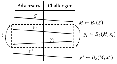
Figure 1: An illustration of Definition 2.2. The adversary wins if $y^{*}=1{\;\;\wedge\;\;}x^{*}\notin S\cup\{x_{1},\ldots,x_{t}\}$.

Unsteady representations.

When the Bloom filter has an unsteady representation, then the algorithm ${\mathbf{B}}_{2}$ is randomized and moreover can change the representation ${M}$. That is, ${\mathbf{B}}_{2}$ is a query algorithm that outputs the response to the query as well as a new representation. That is, the data structure has an internal state that might be changed with each query and the user can perform queries to this data structure. Thus, the user or the adversary do not interact directly with ${\mathbf{B}}_{2}({M},\cdot)$ but with an interface $Q(\cdot)$ (initialized with some ${M}^{*}$) that on query $x$ updates its representation ${M}$ and outputs only the response to the query (i.e., it cannot issue successive queries to the same memory representation but to one that keeps changing). Formally, $Q(\cdot)$ is with ${M}^{*}$ and at each point in time has a memory $M$. Then, on input $x$ is acts as follows:

The interface $Q(x)$:

1. $({M}^{\prime},y)\leftarrow{\mathbf{B}}_{2}({M},x)$.

2. ${M}\leftarrow{M}^{\prime}$.

3. Output $y$.

We define a variant of the above interface, denoted by $Q(x;x_{1},\ldots,x_{t})$ (initialized with ${M}^{*}$) as first performing the queries $x_{1},\ldots,x_{t}$ and then performing the query $x$ and output the result on $x$. Formally, we define:

$Q(x;x_{1},\ldots,x_{t})$:

1. For $i=1\ldots t$ query $Q(x_{i})$.

2. Output $Q(x)$.

We define an analog of the original Bloom filter for unsteady representations and then define an adversarial resilient one.

Definition 2.3 (Bloom filter with an unsteady representation).

Let ${\mathbf{B}}=({\mathbf{B}}_{1},{\mathbf{B}}_{2})$ be a pair of probabilistic polynomial-time algorithms such that ${\mathbf{B}}_{1}$ gets as input the set $S$ of size $n$ and outputs a representation ${M}_{0}$, and ${\mathbf{B}}_{2}$ gets as input a representation and query $x$ and outputs a new representation and a response to the query. Let $Q(\cdot)$ be the process initialized with ${M}_{0}$. We say that ${\mathbf{B}}$ is an $(n,\varepsilon)$-Bloom filter (with an unsteady representation) if for any such set $S$ the following two conditions hold:

1. Completeness: For any $x\in S$, for any $t\in\mathbb{N}$ and for any sequence of queries $x_{1},x_{2},\ldots,x_{t}$ we have that $\Pr[Q(x;x_{1},\ldots,x_{t})=1]=1$.

2. Soundness: For any $x\notin S$, for any $t\in\mathbb{N}$ and for any sequence of queries $x_{1},x_{2},\ldots,x_{t}$ we have that $\Pr[Q(x;x_{1},\ldots,x_{t})=1]\leq\varepsilon$,

where the probabilities are taken over the internal randomness of $Q$.

The above definition is for fixed query sequences, where the next definition is for adaptively chosen query sequences.

Definition 2.4 (Adversarial-resilient Bloom filter with an unsteady representation).

Let ${\mathbf{B}}=({\mathbf{B}}_{1},{\mathbf{B}}_{2})$ be an $(n,\varepsilon)$-Bloom filter with an unsteady representation (see Definition 2.3). We say that ${\mathbf{B}}$ is an $(n,t,\varepsilon)$-adversarial resilient Bloom filter (with an unsteady representation) if for any probabilistic polynomial-time adversary $A=(A_{1},A_{2})$ for all large enough $\lambda\in\mathbb{N}$ it holds that:

• Adversarial Resilient: $\Pr[{\sf Challenge}_{A,t}(\lambda)=1]\leq\varepsilon$,

where the probabilities are taken over the internal randomness of ${\mathbf{B}}_{1},{\mathbf{B}}_{2}$ and $A$ and where the random variable ${\sf Challenge}_{A,t}(\lambda)$ is the outcome of the following process:

${\sf Challenge}_{A,t}(\lambda)$:

1. $S\leftarrow A_{1}(1^{\lambda+n\log{u}})$ where $S\subset U$, and $|S|\leq n$.

2. ${M}_{0}\leftarrow{\mathbf{B}}_{1}(S,1^{\lambda+n\log{u}})$.

3. Initialize $Q(\cdot)$ with ${M}_{0}$.

4. $x^{*}\leftarrow A_{2}^{Q(\cdot)}(1^{\lambda+n\log{u}},S)$ where $A_{2}$ performs at most $t$ adaptive queries $x_{1},\ldots,x_{t}$ to $Q(\cdot)$.

5. If $x^{*}\notin S\cup\{x_{1},\ldots,x_{t}\}$ and $Q(x^{*})=1$ output 1, otherwise output 0.

If ${\mathbf{B}}$ is not $(n,t,\varepsilon)$-resilient then we say there exists an adversary $A$ that can $(n,t,\varepsilon)$-attack ${\mathbf{B}}$. If ${\mathbf{B}}$ is resilient for any polynomial number of queries we say it is strongly resilient:

Definition 2.5 (Strongly resilient).

For a security parameter $\lambda$, we say that ${\mathbf{B}}$ is an $(n,\varepsilon)$-strongly resilient Bloom filter, if for any polynomial $t=t(\lambda,n)$ it holds that ${\mathbf{B}}$ is an $(n,t,\varepsilon)$-adversarial resilient Bloom filter.

Remark 2.6 (Access to the set $S$).

Notice that in Definitions 2.2 and 2.4 the adversary $A_{1}$ chooses the set $S$, and then the adversary $A_{2}$ gets the set $S$ as an additional input. This strengthens the definition of the resilient Bloom filter such that even given the set $S$ it is hard to find false positives. An alternative definition might be to not give the adversary $A_{2}$ the set. However, our results of Theorem 1.1 hold even if the adversary does not get the set. That is, the algorithm that predicts a false positive makes no use of the set $S$. Moreover, the construction in Theorem 1.2 holds in both cases, even against adversaries that do get the set.

An important parameter is the memory use of a Bloom filter ${\mathbf{B}}$. We say ${\mathbf{B}}$ uses $m=m(n,\lambda,\varepsilon)$ bits of memory if for any set $S$ of size $n$ the largest representation is of size at most $m$. The desired properties of Bloom filters is to have $m$ as small as possible and to answer membership queries as fast as possible. Let ${\mathbf{B}}$ be a $(n,\varepsilon)$-Bloom filter that uses $m$ bits of memory. Carter et al. [CFG⁺78] (see also [DP08] for further details) proved a lower bound on the memory use of any Bloom filter showing that if $u>n^{2}/\varepsilon$ then $m\geq n\log{\frac{1}{\varepsilon}}$ (or written equivalently as $\varepsilon\geq 2^{-\frac{m}{n}}$). This leads us to define the minimal error of ${\mathbf{B}}$.

Definition 2.7 (Minimal error).

Let ${\mathbf{B}}$ be an $(n,\varepsilon)$-Bloom filter that uses $m$ bits of memory. We say that $\varepsilon_{0}=2^{-\frac{m}{n}}$ is the minimal error of ${\mathbf{B}}$.

Note that using the lower bound of [CFG⁺78] we get that for any $(n,\varepsilon)$-Bloom filter its minimal error $\varepsilon_{0}$ always satisfies $\varepsilon_{0}\leq\varepsilon$. For technical reasons, we will have a slightly different condition on the size of the universe, and we require that $u=\Omega(m/\varepsilon_{0}^{2})$. Moreover, if $u$ is super-polynomial in $n$, and $\varepsilon$ is negligible in $n$ then any polynomial-time adversary has only negligible chance in finding any false positive, and again we say that the Bloom filter is trivial.

Definition 2.8 (Non-trivial Bloom filter).

Let ${\mathbf{B}}$ be an $(n,\varepsilon)$-Bloom filter that uses $m$ bits of memory and let $\varepsilon_{0}$ be the minimal error of ${\mathbf{B}}$ (see Definition 2.7). We say that ${\mathbf{B}}$ is non-trivial if for all constants $a>0$ it holds that $u>\frac{a\cdot m}{\varepsilon_{0}^{2}}$ and there exists a constant $c$ such that $\varepsilon_{0}>\frac{1}{n^{c}}$.

3 Our Techniques

3.1 One-Way Functions and Adversarial Resilient Bloom Filters

We present the main ideas and techniques of the equivalence of adversarial resilient Bloom filters and one-way functions (i.e., the proof of Theorems 1.1 and 1.2). The simpler direction is showing that the existence of one-way functions implies the existence of adversarial resilient Bloom filters. Actually, we show that any Bloom filter can be efficiently transformed to be adversarial resilient with essentially the same amount of memory. The idea is simple and works in general for other data structures as well: apply a pseudo-random permutation of the input and then send it to the original Bloom filter. The point is that an adversary has almost no advantage in choosing the inputs adaptively, as they are all randomized by the permutation, while the correctness properties remain under the permutation.

The other direction is more challenging. We show that if one-way functions do not exist then any non-trivial Bloom filter can be “attacked” by an efficient adversary. That is, the adversary performs a sequence of queries and then outputs an element $x^{*}$ (that was not queried before) which is a false positive with high probability. We give two proofs: One for the case where the Bloom filter has a steady representation and one for an unsteady representation.

The main idea is that although we are given only oracle access to the Bloom filter, we are able to construct an (approximate) simulation of it. We use techniques from machine learning to (efficiently) ‘learn’ the internal memory of the Bloom filter, and construct the simulation. The learning task for steady and unsteady Bloom filters is quite different and each yield a simulation with different guarantees. Then we show how to exploit each simulation to find false positives without querying the real Bloom filter.

In the steady case, we state the learning process as a ‘PAC learning’ [Val84] problem. We use what’s known as ‘Occam’s Razor’ which states that any hypothesis consistent on a large enough random training set will have a small error. Finally, we show that since we assume that one-way functions do not exist, we are able to find a consistent hypothesis in polynomial time. Since the error is small, the set of false positive elements defined by the real Bloom filter is approximately the same set of false positive elements defined by the simulator.

Handling Bloom filters with an unsteady representation is much more complex. Recall that such Bloom filters are allowed to randomly change their internal representation after each query. In this case, we are trying to learn a distribution that might change after each sample. We describe two examples of Bloom filters with unsteady representations which seem to capture the main difficulties of the unsteady case.

The first example considers any ordinary Bloom filter with error rate $\varepsilon/2$, where we modify the query algorithm to first answer ‘1’ with probability $\varepsilon/2$ and otherwise continue with its original behavior. The resulting Bloom filter has an error rate of $\varepsilon$. However, its behavior is tricky: When observing its responses, elements can alternate between being false positive and negatives, which makes the learning task much harder.

The second example consists of two ordinary Bloom filters with error rate $\varepsilon$, both initialized with the set $S$. At the beginning, only the first Bloom filter is used, and after a number of queries (which may be chosen randomly) only the second one is used. Thus, when switching to the second Bloom filter the set of false positives changes completely. Notice that while first Bloom filter was used exclusively, no information was leaked about the second. This example proves that any algorithm trying to ‘learn’ the memory of the Bloom filter cannot perform a fixed number of samples (as does our learning algorithm for the steady representation case).

To handle these examples, we apply the framework of adaptively changing distributions (ACDs) presented by Naor and Rothblum [NR06], which models the task of learning distributions that can adaptively change after each sample was studied. Their main result is that if one-way functions do not exist then there exists an efficient learning algorithm that can approximate the next activation of the ACD, that is, produce a distribution that is statistically close to the distribution of the next activation of the ACD. We show how to facilitate (a slightly modified version of) this algorithm to learn the unsteady Bloom filter and construct a simulation. One of the main difficulties is that since we get only a statistical distance guarantee, a false positive for the simulation need not be a false positive for the real Bloom filter. Nevertheless, we show how to estimate whether an element is a false positive in the real Bloom filter.

3.2 Computationally Unbounded Adversaries

In Theorem 1.3 we construct a Bloom Filter that is resilient against any unbounded adversary for a given number ($t$) of queries. One immediate solution would be to imitate the construction of the computationally bounded case while replacing the pseudo-random permutation with a $k=(t+n)$-wise independent hash function. Then, any set of $t$ queries along with the $n$ elements of the set would behave as truly random under the hash function. The problem with this approach is that the representation of the hash function is too large: It is $O(k\log{|U|})$ which is more than the number of bits needed for a precise representation of the set $S$. Turning to almost $k$-wise independence does not help either. First, the memory will still be too large (it can be reduced to $O(n\log{n}\log{\frac{1}{\varepsilon}}+t\log{n}\log{\frac{1}{\varepsilon}})$ bits) and second, we get that only sets chosen in advance will act as random, where the point of an adversarial resilient Bloom filter is to handle adaptively chosen sets.

Carter et al. [CFG⁺78] presented a general transformation from any exact dictionary to a Bloom filter. The idea was simple: storing $x$ in the Bloom filter translates to storing $g(x)$ in a dictionary for some (universal) hash function $g:U\rightarrow V$, where $|V|=\frac{n}{\varepsilon}$. The choice of the hash function and underlying dictionary are important as they determine the performance and memory size of the Bloom filter. Notice that, at this point replacing $g$ with a $k=(t+n)$-wise independent hash function (or an almost $k$-independent hash function) yields the same problems discussed above. Nevertheless, this is the starting point for the construction, and we show how to overcome these issues. Specifically, we combine two main ingredients: Cuckoo hashing and a highly independent hash function tailored for this construction.

For the underlying dictionary in the transformation, we use the Cuckoo hashing construction [PR04, Pag08]. Using cuckoo hashing as the underlying dictionary was already shown to yield good constructions for Bloom filters by Pagh et al. [PPR05] and Arbitman et al. [ANS10]. Among the many advantages of Cuckoo hashing (e.g., succinct memory representation, constant lookup time) is the simplicity of its structure. It consists of two tables $T_{1}$ and $T_{2}$ and two hash functions $h_{1}$ and $h_{2}$ and each element $x$ in the Cuckoo dictionary resides in either $T_{1}[h_{1}(x)]$ or $T_{2}[h_{2}(x)]$. However, we use this structure a bit differently. Instead of storing $g(x)$ in the dictionary directly (as the reduction of Carter et al. suggests) which would resolve to storing $g(x)$ at either $T_{1}[h_{1}(g(x))]$ or $T_{2}[h_{2}(g(x))]$ we store $g(x)$ at either $T_{1}[h_{1}(x)]$ or $T_{2}[h_{2}(x)]$. That is, we use the full description of $x$ to decide where $x$ is stored but eventually store only a hash of $x$ (namely, $g(x)$). Since each element is compared only with two cells, we can reduce the size of $V$ to $O\left(\frac{1}{\varepsilon}\right)$ (instead of $\frac{n}{\varepsilon}$).

To initialize the hash function $g$, instead of using a universal hash function we use a very high independence function (which in turn is also constructed based on cuckoo hashing) based on the work of Pagh and Pagh [PP08] and Dietzfelbinger and Woelfel [DW03]. They showed how to construct a family $G$ of hash functions so that on any given set of $k$ inputs it behaves like a truly random function with high probability. Furthermore, a function in $G$ can be evaluated in constant time (in the RAM model), and its description can be stored using roughly $O(k\log{|V|})$ bits (where $V$ is the range of the function).

Note that the guarantee of the function acting randomly holds only for sets $S$ of size $k$ that are chosen in advance. In our case, the set is not chosen in advance but rather chosen adaptively and adversarially. However, Berman et al. [BHKN13] showed that the construction of Pagh and Pagh still works even when the set of queries is chosen adaptively.

At this point, one solution would be to use the family of functions $G$ setting $k=t+n$, with the analysis of Berman et al. as the hash function $g$ and the structure of the Cuckoo hashing dictionary. To get an error of $\varepsilon$, we set $|V|=O\left(\log{\frac{1}{\varepsilon}}\right)$ and get an adversarial resilient Bloom filter that is resilient for $t$ queries and uses $O\left(n\log{\frac{1}{\varepsilon}}+t\log{\frac{1}{\varepsilon}}\right)$ bits of memory. However, our goal is to get a memory size of $O\left(n\log{\frac{1}{\varepsilon}}+t\right)$.

To reduce the memory of the Bloom filter even further, we use the family $G$ a bit differently. Let $\ell=O\left(\log{\frac{1}{\varepsilon}}\right)$, and set $k=O\left(t/\ell\right)$. We define the function $g$ to be a concatenation of $\ell$ independent instances $g_{i}$ of functions from $G$, each outputting a single bit ($V=\{0,1\}$). Using the analysis of Berman et al. we get that each of them behaves like a truly random function for any sequence of $k$ adaptively chosen elements. Consider an adversary performing $t$ queries. To see how this composition of hash functions helps reduce the independence needed, consider the comparisons performed in a query between $g(x)$ and some value $y$ being performed bit by bit. Only if the first pair of bits are equal we continue to compare the next pair. The next query continues from the last pair compared, in a cyclic order. For any set of $k$ elements, the probability of the two bits to be equal is $1/2$. Thus, with high probability, only a constant number of bits will be compared during a single query. That is, in each query only a constant number of function $g_{i}$ will be involved and “pay” in their independence, where the rest remain untouched. Altogether, we get that although there are $t$ queries performed, we have $\ell$ different functions and each function $g_{i}$ is involved in at most $O(t/\ell)=k$ queries (with high probability). Thus, the view of each function remains random on these elements. This results in an adversarial resilient Bloom filter that is resilient for $t$ queries and uses only $O(n\log{\frac{1}{\varepsilon}}+k\log{\frac{1}{\varepsilon}})=O(n\log{\frac{1}{\varepsilon}}+t)$ bits of memory.

4 Adversarial Resilient Bloom Filters and One-Way Functions

In this section, we show that adversarial resilient Bloom filters are (existentially) equivalent to one-way functions (see Definition A.1). We begin by showing that if one-way functions do not exist, then any Bloom filter can be “attacked” by an efficient algorithm in a strong sense:

Theorem 4.1.

Let ${\mathbf{B}}=({\mathbf{B}}_{1},{\mathbf{B}}_{2})$ be any non-trivial Bloom filter (possibly with unsteady representation) of $n$ elements that uses $m$ bits of memory and let $\varepsilon_{0}$ be the minimal error of ${\mathbf{B}}$. If one-way functions do not exist, then for any constant $\varepsilon<1$, ${\mathbf{B}}$ is not $(n,t,\varepsilon)$-adversarial resilient for $t=O\left(m/\varepsilon_{0}^{2}\right)$.

We give two different proofs; The first is self-contained (in particular, we do use the Impagliazzo-Luby [IL89] technique of finding a random inverse), but, deals only with Bloom filters with steady representations. The second handles Bloom filters with unsteady representations, and uses the framework of adaptively changing distributions of [NR06].

4.1 A Proof for Bloom Filters with Steady Representations.

Overview:

We prove Theorem 4.1 for Bloom filters with steady representation (see Definition 2.1). Actually, for the steady case the theorem holds even for $t=O\left(m/\varepsilon_{0}\right)$. In both cases, the adversary $A_{1}$ chooses a uniformly random set $S$. Thus, we focus on describing the adversary $A_{2}$.

Assume that there are no one-way functions. We want to construct an adversary that can attack the Bloom filter. We define a function $f$ to be a function that gets a set $S$, random bits $r$, and elements $x_{1},\ldots,x_{t}$, computes ${M}={\mathbf{B}}_{1}(S;r)$ and outputs $x_{1},\ldots,x_{t}$ along with their evaluation on ${\mathbf{B}}_{2}({M},\cdot)$ (i.e. for each element $x_{i}$ the value ${\mathbf{B}}_{2}({M},x_{i})$). Since $f$ is not one-way, there is an efficient algorithm that can invert it with high probability. That is, the algorithm is given a random set of elements labeled with the information whether they are (false) positives or not and it outputs a set $S^{\prime}$ and bits $r^{\prime}$. For ${M}^{\prime}={\mathbf{B}}_{1}(S^{\prime};r^{\prime})$ the function ${\mathbf{B}}_{2}({M}^{\prime},\cdot)$ is consistent with ${\mathbf{B}}_{2}({M},\cdot)$ for all the elements $x_{1},\ldots,x_{t}$. For a large enough set of queries we show that ${\mathbf{B}}_{2}({M}^{\prime},\cdot)$ is actually a good approximation of ${\mathbf{B}}_{2}({M},\cdot)$ as a function from $U$ to $\{0,1\}$.

We use ${\mathbf{B}}_{2}({M}^{\prime},\cdot)$ to find an input $x^{*}\not\in S$ such that ${\mathbf{B}}_{2}({M}^{\prime},x^{*})=1$ and show that ${\mathbf{B}}_{2}({M},x^{*})=1$ as well (with high probability). This contradicts ${\mathbf{B}}$ being adversarial-resilient and proves that $f$ is a (weak) one-way function (see Definition A.2).

Proof of Theorem 4.1(for the steady case)..

Let ${\mathbf{B}}=({\mathbf{B}}_{1},{\mathbf{B}}_{2})$ be an adversarial-resilient Bloom filter (see Definition 2.2) that uses $m$ bits of memory, initialized with a random set $S$ of size $n$, and let ${M}={\mathbf{B}}_{1}(S)$ be its representation. Assume that one-way functions do not exist. Our goal is to construct an algorithm that, given access to ${\mathbf{B}}_{2}(M,\cdot)$, finds an element $x^{*}\notin S$ that is a false positive with probability greater than $\varepsilon$. For the simplicity of presentation, we assume $\varepsilon\leq 2/3$ (for other values of $\varepsilon$ the same proof works while adjusting the constants appropriately). We need to show an attack on infinitely many $n$’s, and thus throughout the proof we assume that $n$ and $m$ are large enough. We describe the function $f$ (which we intend to invert).

The Function $f$.

The function $f$ takes $N=\log{u\choose n}+r(n)+t\log{u}$ bits as inputs where $r(n)$ is the number of random coins that ${\mathbf{B}}_{1}$ uses ($r(n)$ is polynomial since ${\mathbf{B}}_{1}$ runs in polynomial time) and $t=\frac{200m}{\varepsilon_{0}}$. The function $f$ uses the first $\log{u\choose n}$ bits to sample a set $S$ of size $n$, the next $r(n)$ bits (denoted by $r$) are used to run ${\mathbf{B}}_{1}$ on $S$ and get ${M}^{S}_{r}={\mathbf{B}}_{1}(S;r)$. The last $t\log{u}$ bits are interpreted as $t$ elements of $U$ denoted $x_{1},\ldots,x_{t}$. The output of $f$ is a sequence of these elements along with their evaluation by ${\mathbf{B}}_{2}({M}^{S}_{r},\cdot)$. Formally, the definition of $f$ is:

$$f(S,r,x_{1},\ldots,x_{t})=x_{1},\ldots,x_{t},{\mathbf{B}}_{2}({M}^{S}_{r},x_{1}),\ldots,{\mathbf{B}}_{2}({M}^{S}_{r},x_{t})$$

where ${M}^{S}_{r}={\mathbf{B}}_{1}(S;r)$.

It is easy to see that $f$ is polynomial-time computable. Moreover, we can obtain the output of $f$ on a uniform input by sampling $x_{1},\ldots,x_{t}$ and querying the oracle ${\mathbf{B}}_{2}({M},\cdot)$ on these elements. As shown before (see [Gol01] Section 2.3), if one-way functions do not exist then weak one-way functions (see Definition A.2) also do not exist. Thus, we can assume that $f$ is not weakly one-way. In particular, we know that there exists a polynomial-time algorithm $A$ that inverts $f$ with probability at least $1-1/100$. That is:

$$\Pr[f(A(f(S,r,x_{1},\ldots,x_{t})))=f(S,r,x_{1},\ldots,x_{t})]\geq 1-1/100.$$

Using $A$ we construct an algorithm Attack that will find a false positive $x^{*}$ using $t$ queries with probability $2/3$. The description of the algorithm is given in Figure 2.

The Algorithm Attack Given: Oracle access to the query algorithm ${\mathbf{B}}_{2}({M},\cdot)$. The set $S$. Input: $1^{\lambda},n,m,u$. 1. For $i\in[t]$ sample $x_{i}\in U$ uniformly at random and query $y_{i}={\mathbf{B}}_{2}({M},x_{i})$. 2. Run $A$ (the inverter of $f$) on $(x_{1},\ldots,x_{t},y_{1},\ldots,y_{t})$ and $1^{\lambda}$ to get an inverse $(S^{\prime},r^{\prime},x_{1},\ldots,x_{t})$. 3. Compute ${M}^{\prime}={\mathbf{B}}_{1}(S^{\prime};r^{\prime})$. 4. Do $k=\frac{200}{\varepsilon_{0}}$ times: (a) Sample $x^{*}\in U\setminus\{x_{1},\dots,x_{t}\}\cup S$ uniformly at random. (b) If ${\mathbf{B}}_{2}({M}^{\prime},x^{*})=1$ output $x^{*}$ and HALT. 5. Output an arbitrary $x^{*}\in U$.

Figure 2: The description of the algorithm Attack.

We need to show that the success probability of Attack is more than $2/3$. That is, if $x^{*}$ is the output of the Attack algorithm then we want to show that $\Pr[{\mathbf{B}}_{2}({M},x^{*})=1]\geq 2/3$. Our first step is showing that if $A$ successfully inverts $f$ then with high probability the resulting ${M}^{\prime}$ defines a function that agrees with ${\mathbf{B}}_{2}({M},\cdot)$ on almost all points. For any representations ${M},{M}^{\prime}$ define their error by:

$$\textsf{err}({M},{M}^{\prime}):=\Pr_{x\in U}[{\mathbf{B}}_{2}({M},x)\neq{\mathbf{B}}_{2}({M}^{\prime},x)],$$

where $x$ is chosen uniformly at random from $U$. Using this notation we prove the following claim which is very similar to what is known as “Occam’s Razor” in learning theory [BEHW89].

Claim 4.2.

Let $t=\frac{1000m}{\varepsilon_{0}}$. Then, for any representation ${M}$, over the random choices of $x_{1},\ldots,x_{t}$, the probability that there exists a representation ${M}^{\prime}$ that is consistent with ${M}$ (i.e., that for $i\in[t]$, ${\mathbf{B}}_{2}({M},x_{i})={\mathbf{B}}_{2}({M}^{\prime},x_{i})$) and $\textsf{err}({M},{M}^{\prime})>\frac{\varepsilon_{0}}{100}$ is at most $1/100$.

Proof.

Fix ${M}$ and consider any ${M}^{\prime}$ such that $err({M},{M}^{\prime})>\varepsilon_{0}/100$. We want to bound from above the probability over the choice of $x_{i}$’s that ${M}^{\prime}$ is consistent with ${M}$ on $x_{1},\ldots,x_{t}$. From the independence of the choice of the $x_{i}$’s we get that

$$\Pr_{x_{1},\ldots,x_{t}}\left[\forall i\in[t]\colon{\mathbf{B}}_{2}({M},x_{i})={\mathbf{B}}_{2}({M}^{\prime},x_{i})\right]\leq\left(1-\frac{\varepsilon_{0}}{100}\right)^{t}.$$

Since the data structure uses $m$ bits of memory, there are at most $2^{m}$ possible representations and at most $2^{m}$ candidates for ${M}^{\prime}$. Taking a union bound over the all candidates and for $t=\frac{800m}{\varepsilon_{0}}$ we get that the probability that there exists such a ${M}^{\prime}$ is:

$$\Pr_{x_{1},\dots,x_{t}}\left[\exists{M}^{\prime}\colon\forall i\in[t],{\mathbf{B}}_{2}({M},x_{i})={\mathbf{B}}_{2}({M}^{\prime},x_{i})\right]\leq 2^{m}\left(1-\frac{\varepsilon_{0}}{100}\right)^{t}\leq 2^{m}\cdot e^{-10m}\leq\frac{1}{100}.$$

By the definition of $f$, if $A$ successfully inverts $f$ then it must output $S^{\prime}$ and $r^{\prime}$ such that ${M}^{\prime}={\mathbf{B}}_{1}(S^{\prime};r^{\prime})$ is a representation that is consistent with ${M}$ on all samples $x_{1},\ldots,x_{t}$. Thus, assuming $A$ inverts successfully we get that the probability that $\textsf{err}({M},{M}^{\prime})>\varepsilon_{0}/100$ is at most $1/100$. ∎

Given that $\textsf{err}({M},{M}^{\prime})\leq\varepsilon_{0}/100$, we want to show that with high probability step 4 will halt (on step 4.b). Define $\mu({M})=\Pr_{x\in U}[{\mathbf{B}}_{2}({M},x)=1]$ to be the fraction of positives (false and true) of ${M}$. The number of false positives might depend on $S$. For instance, a Bloom filter might store the set $S$ precisely if $S$ is some special set fixed in advance, and then $\mu(M)=n$. However, we show that for most sets the fraction of positives must be approximately $\varepsilon_{0}$.

Claim 4.3.

For any Bloom filter with minimal error $\varepsilon_{0}$ it holds that:

$$\Pr_{S}\left[\exists r:\mu\left({M}^{S}_{r}\right)\leq\frac{\varepsilon_{0}}{8}\right]\leq 2^{-n}$$

where the probability is taken over a uniform choice of a set $S$ of size $n$ from the universe $U$.

Proof.

Let $\mathsf{BAD}$ be the set of all sets $S$ such that there exists an $r$ such that $\mu({M}^{S}_{r})\leq\frac{\varepsilon_{0}}{8}$. Since the number of sets $S$ is ${u\choose n}$, we need to show that $|\mathsf{BAD}|\leq 2^{-n}{u\choose n}$. We show this using an encoding argument for $S$. Given $S\in\mathsf{BAD}$ there is an $r$ such that $\mu({M}^{S}_{r})\leq\frac{\varepsilon_{0}}{8}$. Let $\widehat{S}$ be the set of all elements $x$ such that ${\mathbf{B}}_{2}({M}^{S}_{r},x)=1$. Then, $|\widehat{S}|\leq\frac{\varepsilon_{0}u}{8}$, and we can encode the set $S$ relative to $\widehat{S}$ using the representation ${M}^{S}_{r}$: Encode ${M}^{S}_{r}$ and then specify $S$ from all subsets of $\widehat{S}$ of size $n$. This encoding must be more than $\log{|\mathsf{BAD}|}$ bits and hence we get the bound:

$$\log{|\mathsf{BAD}|} \leq m+\log{{{\varepsilon_{0}u/8}\choose n}}\leq m+n\log{\left(\varepsilon_{0}u/8\right)}-n\log{n}+2n\leq-n+\log{{u\choose n}},$$

where the second inequality follows from Lemma A.8. ∎

Assuming that ${M}^{\prime}$ is an approximation of ${M}$, it follows that $\mu({M}^{\prime})\approx\mu({M})$, and therefore in step 4 with high probability we will find an $x^{*}$ such that ${\mathbf{B}}_{2}({M},x^{*})=1$. Namely, we get the following claim.

Claim 4.4.

Assume that $\textsf{err}({M},{M}^{\prime})\leq\varepsilon_{0}/100$ and that $\mu({M})\geq\varepsilon_{0}/8$. Then, with probability at least $1-1/100$ the algorithm Attack will halt on step 4, where the probability is taken over the internal randomness of Attack and over the random choices of $x_{1},\ldots,x_{t}$.

Proof.

Recall that ${\mathbf{B}}$ is non-trivial and by definition, we have that $\varepsilon_{0}>am/u$ (for any constant $a$) and that there exists a constant $c\geq 1$ such that $\varepsilon>1/n^{c}$. Since $\textsf{err}({M}^{\prime},{M})\leq\varepsilon_{0}/100$ and $\mu({M})\geq\varepsilon_{0}/8$ we get that

$$\mu({M}^{\prime})\geq\frac{\varepsilon_{0}}{8}-\frac{\varepsilon_{0}}{100}>\frac{\varepsilon_{0}}{10}.$$

Let $\widehat{S^{\prime}}=\{x:{\mathbf{B}}_{2}({M}^{\prime},x)=1\}$ be the set of positives (false and true) relative to $M^{\prime}$. Let $\mathcal{X}=\{x_{1},\ldots,x_{t}\}$ be a multiset of the $t$ elements sampled by the algorithm. The probability of each element to be sampled from $\widehat{S^{\prime}}$ is $\mu({M}^{\prime})$, and thus the expectation is:

$$\mathop{\mathbb{E}}\left[|\widehat{S^{\prime}}\cap\mathcal{X}|\right]=t\cdot\mu({M}^{\prime})\geq\frac{1000m}{\varepsilon_{0}}\cdot\frac{\varepsilon_{0}}{10}=100m.$$

By a Chernoff bound we get that:

$$\Pr\left[|\widehat{S^{\prime}}\cap\mathcal{X}|<200m\right]>1-e^{-\Omega\left(m\right)}.$$

Thus, choosing a large enough constant $a$ we get that

$$|\widehat{S^{\prime}}\setminus(\mathcal{X}\cup S)|\geq|\widehat{S^{\prime}}|-|\widehat{S^{\prime}}\cap\mathcal{X}|-|S|\geq u\cdot\mu(M^{\prime})-200m-n\geq\frac{u\varepsilon_{0}}{10}-200m-n.$$

Thus, we can bound the probability of sampling a successful $x^{*}$

$$\Pr_{x^{*}\in U\setminus\{x_{1},\dots,x_{t}\}\cup S}[x^{*}\in\widehat{S^{\prime}}]\geq\frac{|\widehat{S^{\prime}}\setminus(\mathcal{X}\cup S)|}{u}\geq\frac{\varepsilon_{0}}{10}-\frac{200m}{u}-n/u\geq\frac{\varepsilon_{0}}{10}-\frac{\varepsilon_{0}}{20}=\frac{\varepsilon_{0}}{20},$$

where the last inequality holds since $u>\frac{am}{\varepsilon_{0}}$ for any constant $a>0$. That is, the probability of failing is at most $1-\varepsilon_{0}/20$ and thus the probability of failing in all $k=\frac{100}{\varepsilon_{0}}$ attempts is at most

$$\left(1-\frac{\varepsilon_{0}}{20}\right)^{k}=\left(1-\frac{\varepsilon_{0}}{20}\right)^{\frac{200}{\varepsilon_{0}}}<1/100,$$

and the claim follows.

∎

Assume that we found a random element $x^{*}$ that was never queried before such that ${\mathbf{B}}_{2}({M}^{\prime},x^{*})=1$. Since $\textsf{err}({M}^{\prime},{M})\leq\varepsilon/100$ we have that

$$\Pr_{x}[{\mathbf{B}}_{2}({M},x^{*})=0~{}\mid~{}{\mathbf{B}}_{2}({M}^{\prime},x^{*})=1]\leq 1/100.$$

Altogether, taking a union bound on all the failure points we get that the probability of Attack to fail is at most $4/100<1/3$ as required. ∎

4.2 Handling Unsteady Bloom Filters

In the previous section, we have given a proof for Theorem 4.1 for any steady Bloom filter. In this section, we describe the proof of the theorem that handles Bloom filters with an unsteady representation as well. A Bloom filter with an unsteady representation (see Definition 2.3) has a randomized query algorithm and may change the underlying representation after each query. We want to show that if one-way functions do not exist then we can construct an adversary, Attack, that ‘attacks’ this Bloom filter.

Hard-core Positives.

Let ${\mathbf{B}}=({\mathbf{B}}_{1},{\mathbf{B}}_{2})$ be an $(n,\varepsilon)$-Bloom filter with an unsteady representation that uses $m$ bits of memory (see Definition 2.3). Let ${M}$ and ${M}^{\prime}$ be two representations of a set $S$ generated by ${\mathbf{B}}_{1}$. In the previous proof in Section 4.1, given a representation ${M}$ we considered ${\mathbf{B}}_{2}(M,\cdot)$ as a boolean function. We defined the function $\mu({M})$ to measure the number of positives in ${\mathbf{B}}_{2}(M,\cdot)$ and we defined the error between two representations $\textsf{err}({M},{M}^{\prime})$ to measure the fraction of inputs that the two boolean functions agree on. These definitions make sense only when ${\mathbf{B}}_{2}$ is deterministic and does not change the representation. However, in the case of Bloom filters with unsteady representations, we need to modify the definitions to have new meanings.

Given a representation ${M}$ consider the query interface $Q(\cdot)$ initialized with ${M}$. For an element $x$, the probability of $x$ being a false positive is $\Pr[Q(x)=1]=\Pr[{\mathbf{B}}_{2}(M,x)=1]$. Recall that after querying $Q(\cdot)$, the interface updates its representation and the probability of $x$ being a false positive might change (it could be higher or lower). We say that $x$ is a ‘hard-core positive’ if after any arbitrary sequence of queries we have that $\Pr[Q(x)=1]=1$. That is, the query interface will always respond with a ‘1’ on $x$ even after any sequence of queries. Then, we define $\mu({M})$ to be the set of hard-core positive elements in $U$. Note that over the time, the size of $\mu({M})$ might grow, but by definition it can never become smaller. We observe that what Claim 4.3 actually proves is that for almost all sets $S$ the number of hard-core positives is large.

The Distribution $D_{{M}}$.

As we can no longer talk about the function ${\mathbf{B}}_{2}({M},\cdot)$ we turn to talk about distributions. For any representation ${M}$, define the distribution $D_{{M}}$: Sample $k$ elements at random $x_{1},\ldots,x_{k}$ ($k$ will be determined later), and output $(x_{1},\ldots,x_{k},Q(x_{1}),\dots,Q(x_{k}))$. Note that the underlying representation ${M}$ changes after each query. The precise algorithm of $D_{{M}}$ is given by:

$D_{M}$:

1. Sample $x_{1},\ldots,x_{k}\in U$ uniformly at random.

2. For $i=1,\ldots,k$: compute $y_{i}=Q(x_{i})$.

3. Output $(x_{1},\ldots,x_{k},y_{1},\dots,y_{k})$.

Let ${M}_{0}$ be a representation of a random set $S$ generated by ${\mathbf{B}}_{1}$, and let $\varepsilon_{0}$ be the minimal error of ${\mathbf{B}}$. Let $D_{{M}_{0}}$ be the distribution described above using $M_{0}$. Assume that one-way functions do not exist. Our goal is to construct an algorithm Attack that will ‘attack’ ${\mathbf{B}}$, that is, it is given access to $Q(\cdot)$ initialized with ${M}_{0}$ (${M}_{0}$ is secret and not known to Attack) and it must find a non-set element $x^{*}$ such that $\Pr[Q(x^{*})=1]\geq 2/3$.

Consider the distribution $D_{{M}_{0}}$, and notice that given access to $Q(\cdot)$ we can perform a single sample from $D_{{M}_{0}}$: sample $k$ random elements and query $Q(\cdot)$ on these elements. Let $M_{1}$ be the random variable of the resulting representation after the sample. Now, we can sample from the distribution $D_{{M}_{1}}$, and then $D_{{M}_{2}}$ and so on. We begin by describing a simplified version of the proof where we assume that ${M}_{0}$ is known to the adversary. This version seems to capture the main ideas. Then, in Section 4.3 we show how to eliminate this assumption and get a full proof.

Attacking when ${M}_{0}$ is known.

Suppose that after activating $D_{{M}_{0}}$ for $r$ rounds we are given the initial state ${M}_{0}$ (of course, in the actual execution ${M}_{0}$ is secret and later we show how to overcome this assumption). Let $p_{1},\ldots,p_{r}$ be the outputs of the rounds (that is, $p_{i}=(x_{1},\ldots,x_{k},y_{1},\ldots,y_{k})$). For a specific output $p_{i}$ we say that $x_{j}$ was labeled ‘1’ if $y_{j}=1$.

We define a few variants of the distribution $D_{{M}_{0}}$. These variants all have same output format (i.e., they output $(x_{1},\ldots,x_{k},y_{1},\ldots,y_{k})$), and differ only by their given probabilities. Denote by $D_{{M}_{0}}(p_{0},\ldots,p_{r})$ the distribution over the ${(r+1)}\textsuperscript{th}$ activation of $D_{{M}_{0}}$ conditioned on the first $r$ activations resulting in the states $p_{0},\ldots,p_{r}$. Computational issues aside, the distribution $D_{{M}_{0}}(p_{0},\ldots,p_{r})$ can be sampled by enumerating all random strings such that when used to run $D_{{M}_{0}}$ yield the output $p_{0},\ldots,p_{r}$, sampling one of them at random, using it to run $D_{{M}_{0}}$ and outputting $p_{r+1}$.

Moreover, define $D_{{M}_{0}}(p_{0},\ldots,p_{r};x_{1},\ldots,x_{k})$ to be the same distribution as $D_{{M}_{0}}(p_{0},\ldots,p_{r})$, however, we further conditioned that its final output $p_{r+1}$ satisfy $p_{r+1}=x_{1},\ldots,x_{k},y_{1},\ldots,y_{k}$. That is, we condition the $x^{\prime}s$ and the distribution is only over the $y_{i}$’s. Finally, we define $D(p_{0},\ldots,p_{r})$ to be the same distribution as $D_{{M}_{0}}(p_{0},\ldots,p_{r})$ only where the representation ${M}_{0}$ is also chosen at random (according to ${\mathbf{B}}_{1}(S)$).

We define an (inefficient) adversary Attack in Figure 3 that (given ${M}_{0}$) can attack the Bloom filter, that is, find an element $x^{*}$ that was not queried before and is a false positive with high probability (the final adversary will be efficient).

The Algorithm Attack Given: The representation ${M}_{0}$, states $p_{1},\ldots,p_{r}$ and oracle access to $Q(\cdot)$. 1. Sample $x_{1},\ldots,x_{k}\in U$ at random. 2. For $i\in[\ell]$ sample $D_{{M}_{0}}(p_{0},\ldots,p_{r};x_{1},\ldots,x_{k})$ to get $y_{i1},\ldots,y_{ik}$. 3. If there exists an index $j\in[k]$ such that for all $i\in[\ell]$ it holds that $y_{ij}=1$: (a) Set $x^{*}=x_{j}$. (b) Query $Q(x_{1}),\ldots,Q(x_{j-1})$. (c) Output $x^{*}$ and halt. 4. Otherwise set $x^{*}$ to be an arbitrary element in $U$.

Figure 3: The description of the algorithm Attack.

Set $k=160/\varepsilon_{0}$ and $\ell=100k$. Then we get the following claims. First, we show that there will be a common element $x_{j}$ (that is, the condition in line 3 will hold).

Claim 4.5.

With probability $99/100$ there exist a $1\leq j\leq k$ such that for all $i\in[\ell]$ it holds that $y_{ij}=1$, where the probability is over the random choice of $S$ and $x_{1},\ldots,x_{k}$.

Proof.

Let ${M}_{r}$ be the resulting representation of the ${r}\textsuperscript{th}$ activation of $D_{{M}_{0}}(p_{0},\ldots,p_{r};x_{1},\ldots,x_{k})$. We have seen that with probability $1-2^{-n}$ over the choice of $S$ for any ${M}_{0}$ we have that the set of hard-core positives satisfy $|\mu({M}_{0})|\geq\varepsilon_{0}/16$. By the definition of the hard-core positives, the set $\mu({M}_{0})$ may only grow after each query. Thus, for each sample from $D_{{M}_{0}}(p_{0},\ldots,p_{r};x_{1},\ldots,x_{k})$ we have that $\mu({M}_{0})\subseteq\mu({M}_{r})$. If $x_{j}\in\mu({M}_{0})$ then $x_{j}\in\mu({M}_{r})$ and thus $y_{ij}=1$ for all $i\in[\ell]$. The probability that all elements $x_{1},\ldots,x_{k}$ are sampled outside the set $\mu({M}_{0})$ is at most $(1-\varepsilon_{0}/16)^{k}\leq e^{-10}$ (over the random choices of the elements). All together we get that probability of choosing a ‘good’ $S$ and a ‘good’ sequence $x_{1},\ldots,x_{t}$ is at least $1-2^{-n}+e^{-10}\geq 99/100$. ∎

Claim 4.6.

Let ${M}_{r}$ be the underlying representation of the interface $Q(\cdot)$ at the time right after sampling $p_{0},\ldots,p_{r}$. Then, with probability at least $98/100$ the algorithm Attack outputs an element $x^{*}$ such that $Q(x^{*})=1$, where the probability is taken over the randomness of Attack, the sampling of $p_{0},\ldots,p_{r}$, and ${\mathbf{B}}$.

Proof.

Consider the distribution $D_{{M}_{0}}(p_{0},\ldots,p_{r};x_{1},\ldots,x_{k})$ to work in two phases: First, a representation ${M}$ is sampled conditioned on starting from ${M}_{0}$ and outputting the states $p_{0},\ldots,p_{r}$ and then we compute $y_{j}={\mathbf{B}}_{2}({M},x_{j})$. Let ${M}^{\prime}_{1},\ldots,{M}^{\prime}_{\ell}$ be the representations chosen during the run of Attack. Note that $M_{r}$ is chosen from the same distribution that ${M}^{\prime}_{1},\ldots,{M}^{\prime}_{\ell}$ are sampled from. Thus, we can think of ${M}_{r}$ as being picked after the choice of $x_{1},\ldots,x_{k}$. That is, we sample ${M}^{\prime}_{1},\ldots,{M}^{\prime}_{\ell+1}$, and choose one of them at random to be ${M}_{r}$, and the rest are relabeled as ${M}^{\prime}_{1},\ldots,{M}^{\prime}_{\ell}$. Now, for any $x_{j}$, the probability that for all $i$, ${M}^{\prime}_{i}$ will answer ‘1’ on $x_{j}$ but ${M}_{r}$ will answer ‘0’ on $x_{j}$ is at most $1/\ell$. Thus, the probability that there exist any such $x_{j}$ is at most $\frac{k}{\ell}=\frac{k}{100k}=1/100$. Altogether, the probability that $A$ finds such an $x_{j}$ that is always labeled ‘1’ and that ${M}_{r}$ answers ‘1’ on it, is at least $99/100-1/100=98/100$. ∎

Finally, we claim that $x^{*}$ is truly a false positive, that is $x^{*}\notin S$ and that $x^{*}$ is not one of the previous $t$ queries. By our bound on $t$ we get that $n+t=O(m/\varepsilon_{0}^{2})$. Since the Bloom filter is non-trivial, we get that $u>am/\varepsilon_{0}^{2}$ for any constant $a$. Therefore, the probability that $x^{*}$ is not a new false positive is negligible.

We are left to show how to construct the algorithm Attack so that it will run in polynomial-time and perform the same tasks without knowing ${M}_{0}$. Note that our only use of ${M}_{0}$ was to sample from $D_{{M}_{0}}(p_{0},\ldots,p_{r};x_{1},\ldots,x_{k})$ without changing it (since it changes after each sample). The goal is to observe outputs of this distribution until we have enough information about it, such that we can simulate it without changing its state. One difficulty (which was discussed in Section 3), is that the number of samples $r$ must be chosen as a function of the samples and cannot be fixed in advance. Algorithms for such tasks were studied in the framework of Naor and Rothblum [NR06] on adaptively changing distributions.

4.3 Using ACDs

We continue the full proof of Theorem 4.1. First, we give an overview of the framework of adaptively changing distributions of Naor and Rothblum [NR06].

Adaptively Changing Distributions.

An adaptively changing distribution (ACD) is composed of a pair of probabilistic algorithms, one for generating ($G$) and for sampling ($D$). The generation algorithm $G$ receives a public input $x\in\{0,1\}^{n}$ and outputs an initial secret state $s_{0}\in\{0,1\}^{s(n)}$ and a public state $p_{0}$:

$$G\colon R\to S_{p}\times S_{init},$$

where the set of possible public states is denoted by $S_{p}$ and the set of secret states is denoted by $S_{s}$. After running the generation algorithm, we can consecutively activate a sampling algorithm $D$ to generate samples from the adaptively changing distribution. In each activation, $D$ receives as its input a pair of secret and public states, and outputs new secret and public states. Each new state is always a function of the current state and some randomness, which we assume is taken from a set $R$. The states generated by an ACD are determined by the function

$$D\colon S_{p}\times S_{s}\times R\to S_{p}\times S_{s}.$$

When $D$ is activated for the first time, it is run on the initial public and secret states $p_{0}$ and $s_{0}$ respectively, generated by $G$. The public output of the process is a sequence of public states $(x,p_{0},p_{1},\ldots)$.

Learning ACDs:

An algorithm $L$ for learning an ACD $(G,D)$ sees $x$ and $p_{0}$ (which were generated, together with $s_{0}$, by running $G$), and is then allowed to observe $D$ in consecutive activations, seeing only the public states $D$ outputs. The learning algorithm’s goal is to output a hypothesis $h$ on the initial secret state that is functionally equivalent to $s_{0}$ for the next activation of $D$. The requirement is that with probability at least $1-\delta$ (over the random coins of $G$, $D$, and the learning algorithm), the distribution of the next public state, given the past public states and that $h$ was the initial secret output of $G$, is $\varepsilon$-close to the same distribution with $s_{0}$ as the initial secret state (the “real” distribution of $D$’s next public state). Throughout the learning process, the sampling algorithm $D$ is run consecutively, changing the public (and secret) state. Let $p_{i}$ and $s_{i}$ be the public secret states after $D$’s ${i}\textsuperscript{th}$ activation. We refer to the distribution $D^{s_{0}}_{i}(x,p_{0},\dots,p_{i})$ as the distribution on the public state that will be generated by $D$’s next ${(i+1)}\textsuperscript{th}$ activation.

After letting $D$ run for (at most) $r$ steps, $L$ should stop and output some hypothesis $h$ that can be used to generate a distribution that is close to the distribution of $D$’s next public output. We emphasize that $L$ sees only $(x,p_{0},p_{1},\ldots,p_{r})$, while the secret states $(s_{0},s_{1},\ldots,s_{r})$ and the random coins used by $D$ are kept hidden from it. The number of times $D$ is allowed to run ($r$) is determined by the learning algorithm. We say that $L$ is an $(\varepsilon,\delta)$-learning algorithm for $(G,D)$, that uses $r$ rounds, if when run in a learning process for $(G,D)$, $L$ always (for any input $x\in\{0,1\}^{n}$) halts and outputs some hypothesis $h$ that specifies a hypothesis distribution $D_{h}$, such that with probability $1-\delta$ it holds that $\Delta(D^{s_{0}}_{r+1},D_{h})\leq\varepsilon$, where $\Delta$ is the statistical distance between the distributions (see Definition A.4).

We say that an ACD is hard to $(\varepsilon,\delta)$-learn with $r$ samples if no efficient learning algorithm can $(\varepsilon,\delta)$-learn the ACD using $r$ rounds. The main result regarding ACDs that we use is an equivalence between hard-to-learn ACDs and almost one-way functions (where an almost one-way function is a function that are hard to invert for an infinite number of sizes, see Definition A.3.)

Theorem 4.7 ([NR06]).

Almost one-way functions exist if and only if there exists an adaptively changing distribution $(G,D)$ and polynomials $\delta(n)$, $\varepsilon(n)$, such that it is hard to $(\varepsilon(n),\delta(n))$-learn the ACD $(G,D)$ with $O\left(\frac{\log{|S_{init}|}}{\varepsilon^{2}(n)\delta^{4}(n)}\right)$ samples.

The consequence of Theorem 4.7 is that if we assume that one-way functions do not exist, then no ACD is hard to learn. For concreteness, we get that, given an ACD there exists an algorithm $L$ that (for infinitely many input sizes) with probability at least $1-\delta$ performs at most $O\left(\log{|S_{init}|}\right)$ samples and produces an hypothesis $h$ on the initial state and a distribution $D_{h}$ such that the statistical distance between $D_{h}$ and the next activation of the ACD is at most $\varepsilon$. The point is that $D_{h}$ can be (approximately) sampled in polynomial-time.

From Bloom Filters to ACDs.

As one can see, the process of sampling from $D_{{M}_{0}}$ is equivalent to sampling from an ACD defined by $D_{{M}_{0}}$. The secret states are the underlying representations of the Bloom filter, and the initial secret state is ${M}_{0}$. The public states are the outputs of the sampling. Since the Bloom filter uses at most $m$ bits of memory for each representation we have that $|S_{init}|\leq 2^{m}$.

Running the algorithm $L$ on the ACD constructed above, will output a hypothesis ${M}_{h}$ of the initial representation such that the distribution $D_{{M}_{h}}(p_{0},\ldots,p_{r})$ is close (in statistical distance) to the distribution $D_{{M}_{0}}(p_{0},\ldots,p_{r})$. The algorithm’s main goal is to estimate whether the weight (i.e., the probability) of representations ${M}$ according to $D(p_{0},\ldots,p_{i})$ such that $D({M},p_{0},\ldots,p_{i})$ is close to $D({M}_{0};p_{0},\ldots,p_{i})$ is high, and then samples such a representation. The main difficulty of their work is showing that if almost one-way functions do not exist then this estimation of sampling procedures can be implemented efficiently. We slightly modify the algorithm $L$ to output several such hypotheses instead of only one. The overview of the modified algorithm is given below (the only difference from the original algorithm is the number of output hypotheses):

1. For $i\leftarrow 1\ldots r$ do:

   1. Estimate whether the weight of representations ${M}$ according to $D(p_{0},\ldots,p_{i})$ such that $D_{{M}}(p_{0},\ldots,p_{i})$ is close to $D_{{M}_{0}}(p_{0},\ldots,p_{i})$ is high. Namely, estimate if there is a subset $\mathcal{M}\subset S_{init}$ such that $\Pr_{D(p_{0},\ldots,p_{i})}[\mathcal{M}]$ is high and for all $M\in\mathcal{M}$ it holds that $\Delta(D_{{M}}(p_{0},\ldots,p_{i}),D_{{M}_{0}}(p_{0},\ldots,p_{i}))$ is small.

      If the weight estimate is high then (approximately) sample $h_{1},\ldots,h_{\ell}\leftarrow S_{init}$ according to $D(p_{0},\ldots,p_{i})$, output $h_{1},\ldots,h_{\ell}$, and terminate.

   2. Activate $D_{{M}_{i}}$ to sample $p_{i+1}$ and proceed to round $i+1$.

2. Output arbitrarily some ${M}$ and terminate.

We run the modified algorithm $L$ on the ACD defined by $D_{{M}_{0}}$ with parameters $\gamma=\frac{1}{100\ell}$ and $\delta=1/100$ (recall that $k=160/\varepsilon_{0}$ and $\ell=100k$). The output is $h_{1},\ldots,h_{\ell}$ with the property that with probability at least $1-1/100$ for every $i\in[\ell]$ it holds that

$$\Delta\left(D_{{M}_{0}}(p_{0},\ldots,p_{r}),D_{h_{i}}(p_{0},\ldots,p_{r})\right)\leq 1/100.$$

We modify the algorithm Attack such that the ${i}\textsuperscript{th}$ sample from $D_{{M}}(p_{0},\ldots,p_{r};x_{1},\ldots,x_{k})$ is replaced with a sample from $D_{h_{i}}(p_{0},\ldots,p_{r};x_{1},\ldots,x_{k})$. We have shown that the algorithm Attack succeeds given samples from $D_{{M}_{0}}(p_{0},\ldots,p_{r};x_{1},\ldots,x_{k})$. However, now it is given samples from distributions that are only ‘close’ to $D_{{M}_{0}}(p_{0},\ldots,p_{r};x_{1},\ldots,x_{k})$.

Consider these two cases where in one we sample from $D_{{M}_{0}}(p_{0},\ldots,p_{r})$ and in the other we sample from $D_{h_{i}}(p_{0},\ldots,p_{r})$. Each one defines a different distribution, denoted $D^{1}$ and $D^{2}$, respectively. The distribution $D^{1}$ is defined by sampling $x_{1},\ldots,x_{k}$ and then sampling $\ell$ times from $D_{{M}_{0}}(p_{0},\ldots,p_{r};x_{1},\ldots,x_{k})$, and the distribution $D^{2}$ is defined by sampling $x_{1},\ldots,x_{k}$ and then sampling from $D_{h_{i}}(p_{0},\ldots,p_{r};x_{1},\ldots,x_{k})$ for each $i\in[\ell]$.

Since $\Delta(D_{{M}_{0}}(p_{0},\ldots,p_{r}),D_{h_{i}}(p_{0},\ldots,p_{r})\leq\gamma=\frac{1}{100\ell}$ for any $i\in[\ell]$, by the triangle inequality we get that $\Delta(D^{1},D^{2})\leq\ell\gamma=1/100$. Let $\mathsf{BAD}$ be the event the algorithm Attack does not succeed in finding an appropriate $x^{*}$. We have shown that under the first distribution $\Pr_{D^{1}}[\mathsf{BAD}]\leq 2/100$. Moreover, we have shown that with probability $99/100$ we can find a distribution $D^{2}$ such that $\Delta(D^{1},D^{2})\leq 1/100$. Taking a union bound, we get that the probability of the event $\mathsf{BAD}$ under the distribution $D^{2}$ is $\Pr_{D^{2}}[\mathsf{BAD}]\leq 2/100+1/100+1/100\leq 1/3$, as required.

The number of rounds performed by $L$ is $O(m/\gamma)$ and each round we perform $k$ queries. Thus, the total amount of queries is $O(mk/\gamma)=O(m/\varepsilon_{0}^{2})$. As shown before, the probability that $x^{*}$ is not a new false positive is negligible.

4.4 A Construction Using Pseudorandom Permutations.

We have seen that Bloom filters that are adversarial resilient require using one-way functions. To complete the equivalence, we show that cryptographic tools and in particular pseudorandom permutations and functions can be used to construct adversarial resilient Bloom filters. Actually, we show that any Bloom filter can be efficiently transformed to be adversarial resilient with essentially the same amount of memory. The idea is simple and can work in general for other data structures as well: On any input $x$ we compute a pseudorandom permutation of $x$ and send it to the original Bloom filter. Recall that a pseudorandom permutation (PRP) is a keyed family of permutations that a random function from the family is indistinguishable from a truly random permutation given only oracle access to the function.

Theorem 4.8.

Let ${\mathbf{B}}$ be an $(n,\varepsilon)$-Bloom filter using $m$ bits of memory. If pseudorandom permutations exist, then there exists a negligible function ${\mathsf{neg}}(\cdot)$ such that for security parameter $\lambda$ there exists an $(n,\varepsilon+{\mathsf{neg}}(\lambda))$-strongly resilient Bloom filter that uses $m^{\prime}=m+\lambda$ bits of memory.

Proof.

The main idea is to randomize the adversary’s queries by applying a pseudorandom permutation (see Definition A.6) on them; then we may consider the queries as random and not as chosen adaptively by the adversary.

Let ${\mathbf{B}}$ be an $(n,\varepsilon)$-Bloom filter using $m$ bits of memory. We will construct a $(n,\varepsilon+{\mathsf{neg}}(\lambda))$-strongly resilient Bloom filter ${\mathbf{B}}^{\prime}$ as follows: To initialize ${\mathbf{B}}^{\prime}$ on a set $S$ we first choose a key $K\in\{0,1\}^{\lambda}$ for a pseudo-random permutation, PRP, over $\{0,1\}^{\log{u}}$. Let

$$S^{\prime}=\textsf{PRP}_{K}(S)=\{\textsf{PRP}_{K}(x):x\in S\}.$$

Then we initialize ${\mathbf{B}}$ with $S^{\prime}$. For the query algorithm, on input $x$ we output ${\mathbf{B}}(\textsf{PRP}_{K}(x))$. Notice that the only additional memory we need is storing the key $K$ of the PRP which takes $\lambda$ bits. Moreover, the running time of the query algorithm of ${\mathbf{B}}^{\prime}$ is one pseudo-random permutation more than the query time of ${\mathbf{B}}$.

The completeness follows immediately from the completeness of ${\mathbf{B}}$. If $x\in S$ then ${\mathbf{B}}$ was initialized with $\textsf{PRP}_{K}(x)$ and thus when querying on $x$ we will query ${\mathbf{B}}$ on $\textsf{PRP}_{K}(x)$ which will return ‘1’ from the completeness of ${\mathbf{B}}$.

The resilience of the construction follows from a hybrid argument. Let $A$ be an adversary that queries ${\mathbf{B}}^{\prime}$ on $x_{1},\ldots,x_{t}$ and outputs $x$ where $x\notin\{x_{1},\ldots,x_{t}\}$. Consider the experiment where the PRP is replaced with a truly random permutation oracle $R(\cdot)$. Then, since $x$ was not queried before, we know that $R(x)$ is a truly random element that was not queried before, and we can think of it as chosen before the initialization of ${\mathbf{B}}$. From the soundness of ${\mathbf{B}}$ we get that the probability of $x$ being a false positive is at most $\varepsilon$.

We show that $A$ cannot distinguish between the Bloom filter we constructed and our experiment (using a random permutation) by more than a negligible advantage. Suppose that there exists a polynomial $p(\lambda)$ such that $A$ can attack ${\mathbf{B}}^{\prime}$ and find a false positive with probability $\varepsilon+\frac{1}{p(\lambda)}$. We will show that we can use $A$ to construct an algorithm $A_{2}$ that can distinguish between a random oracle and a PRP with non-negligible probability. Run $A$ on ${\mathbf{B}}^{\prime}$ where the PRP is replaced with an oracle that is either random or pseudo-random. Answer ‘1’ if $A$ successfully finds a false positive. Then, we have that

$$\left|\Pr[A_{2}^{R}(1^{\lambda})]-\Pr[A_{2}^{\textsf{PRP}}(\lambda)]\right|\geq\left|\varepsilon-\varepsilon+\frac{1}{p(\lambda)}\right|=\frac{1}{p(\lambda)}$$

which contradicts the indistinguishability of the PRP family.

∎

Constructing Pseudorandom Permutations from One-way Functions.

Pseudorandom permutations have several constructions from one-way functions which target different domains sizes. If the universe is large, one can obtain pseudorandom permutations from pseudorandom functions using the famed Luby-Rackoff construction from pseudorandom functions [LR88, NR99], which in turn can be based on one-way functions.

For smaller domain sizes ($u=|U|$ quite close to $n$) or domains that are not a power of two the problem is a bit more complicated. There has been much attention given to this issue in recent years and Morris and Rogaway [MR14] presented a construction that is computable in expected $O(\log u)$ applications of a pseudorandom function. Alternatively, Stefanov and Shi [SS12] give a construction of small domain pseudorandom permutations, where the asymptotic cost is worse ($\sqrt{u}\log{u}$), however, in practice, it performs very well in common use cases (e.g., when $u\leq 2^{32}$).

The reason we use permutations is to avoid the event of an element $x\not\in S$ colliding with the set $S$ on the pseudorandom function. If one replaces the pseudorandom permutation with a pseudorandom function, then a term of $n/u$, a bound on the probability of this collision, must be added to the false positive error rate; other than that the analysis is the same as in the permutation case. So unless $u$ is close $n$ this additional error might be tolerated, and it is possible to replace the use of the pseudorandom permutation with a pseudorandom function.

Remark 4.9 (Alternatives).

The transformation suggested does not interfere with the internal operation of the Bloom filter implementation and might preserve other properties of the Bloom filter as well. For example, it is applicable when the set is not given in advance but is provided dynamically among the membership queries, and even in the case where the size of the set is not known in advance (as in [PSW13]).

An alternative approach is to replace the hash functions used in ‘traditional’ Bloom filter constructions or those in [PPR05, ANS10] with pseudorandom functions. The potential advantage of doing the analysis per construction is that we may save on the computation. Since many constructions use several hash functions, it might be possible to use the result of a single pseudorandom evaluation to get all the randomness required for all of the hash functions at once.

Notice that, in all the above constructions only the pseudorandom function (permutation) key must remain secret. That is, we get the same security even when the adversary gets the entire memory of the Bloom filter except for the PRF (PRP) key.

5 Computationally Unbounded Adversary

In this section, we extend the discussion of adversarial resilient Bloom filters to ones against computationally unbounded adversaries. First, notice that the attack of Theorem 4.1 holds in this case as well, since an unbounded adversary can invert any function (with probability 1). Formally, we get the following corollary:

Corollary 5.1.

Let ${\mathbf{B}}=({\mathbf{B}}_{1},{\mathbf{B}}_{2})$ be any non-trivial Bloom filter of $n$ elements that uses $m$ bits of memory and let $\varepsilon_{0}$ be the minimal error of ${\mathbf{B}}$. Then for any constant $\varepsilon<1$ there exist a $t$ such that ${\mathbf{B}}$ is not $(n,t,\varepsilon)$-adversarial resilient against unbounded adversaries and $t=O\left(\frac{m}{\varepsilon_{0}^{2}}\right)$.

As we saw, any $(n,\varepsilon)$-Bloom filter must use at least $n\log{\frac{1}{\varepsilon}}$ bits of memory. We show how to construct Bloom Filters that are resilient against unbounded adversaries for $t$ queries while using only $O\left(n\log{\frac{1}{\varepsilon}}+t\right)$ bits of memory.

Theorem 5.2.

For any $n,t\in\mathbb{N}$, and $0<\varepsilon<1/2$ there exists an $(n,t,\varepsilon)$-resilient Bloom filter (against unbounded adversaries) that uses $O(n\log{\frac{1}{\varepsilon}}+t)$ bits of memory and has linear setup time and $O(1)$ worst-case query time.

Our construction uses two main ingredients: Cuckoo hashing and a very high independence hash family $G$. We begin by describing these ingredients.

The Hash Function Family $G$.

Pagh and Pagh [PP08] and Dietzfelbinger and Woelfel [DW03] (see also Aumüller et al. [ADW14]) showed how to construct a family $G$ of hash functions $g:U\to V$ so that on any set of $k$ inputs it behaves like a truly random function with high probability ($1-1/\textsf{poly}(k)$). Furthermore, $g$ can be evaluated in constant time (in the RAM model), and its description can be stored using $(1+\alpha)k\log{|V|}+O(k)$ bits (where here $\alpha$ is an arbitrarily small constant).

Note that the guarantee of $g$ acting as a random function holds for any set $S$ that is chosen in advance. In our case the set is not chosen in advance but chosen adaptively and adversarially. However, Berman et al. [BHKN13] showed that the same line of constructions, starting with Pagh and Pagh, actually holds even when the set of queries is chosen adaptively. That is, for any distinguisher that can adaptively choose $k$ inputs, the advantage of distinguishing a function $g\in_{R}G$ from a truly random function is polynomially small.

Set $\ell=4\log{\frac{1}{\varepsilon}}$. Our function $g$ will be composed of the concatenation of $\ell$ one bit functions $g_{1},g_{2},\ldots,g_{\ell}$ where each $g_{i}$ is selected independently from a family $G$ where $V=\{0,1\}$ and $k=2t/\log{\frac{1}{\varepsilon}}$. For a random $g_{i}\in_{R}G$:

• There is a constant $c$ (which we can choose) so that for any adaptive distinguisher that issues a sequence of $k$ adaptive queries on $g_{i}$ the advantage of distinguishing between $g_{i}$ and an exact $k$-wise independent function $U\to V$ is bounded by $\frac{1}{k^{c}}$.

• $g_{i}$ can be represented using $O(k)$ bits.

• $g_{i}$ can be evaluated in constant time.

Thus, the representation of $g$ requires $O(\ell\cdot k)=O(t)$ bits. The evaluation of $g$ at a given point $x$ takes $O(\ell)=O\left(\log{\frac{1}{\varepsilon}}\right)$ time.

Cuckoo Hashing.

Cuckoo hashing is a data structure for dictionaries introduced by Pagh and Rodler [PR04]. It consists of two tables $T_{1}$ and $T_{2}$, each containing $r$ cells where $r$ is slightly larger than $n$ (that is, $r=(1+\alpha)n$ for some small constant $\alpha$) and two hash functions $h_{1},h_{2}:U\to[r]$. The elements are stored in the two tables so that an element $x$ resides at either $T_{1}[h_{1}(x)]$ or $T_{2}[h_{2}(x)]$. Thus, the lookup procedure consists of one memory accesses to each table plus computing the hash functions. This description ignores insertions, where insertions can be performed in expected constant time (or alternatively, all $n$ elements can be inserted in linear time with high probability).

Our construction of an adversarial resilient Bloom filter is:

Setup.

The input is a set $S$ of size $n$. Sample a function $g$ by sampling $\ell$ functions $g_{i}\in_{R}G$ and initialize a Cuckoo hashing dictionary $D$ of size $n$ (with $\alpha=0.1$) as described above. That is, $D$ has two tables $T_{1}$ and $T_{2}$ each of size $1.1n$, two hash functions $h_{1}$ and $h_{2}$, and each element $x$ will reside at either $T_{1}[h_{1}(x)]$ or $T_{2}[h_{2}(x)]$. Insert the elements of $S$ into $D$. Then, go over the two tables $T_{1}$ and $T_{2}$ and at each cell replace each $x$ with $g(x)$. That is, now for each $x\in S$ we have that $g(x)$ resides at either $T_{1}[h_{1}(x)]$ or $T_{2}[h_{2}(x)]$. Put $\bot$ in the empty locations. The final memory of the Bloom Filter is the memory of $D$ and the representation of $g$. The dictionary $D$ consists of $O(n)$ cells, each of size $|g(x)|=O(\log{\frac{1}{\varepsilon}})$ bits and therefore $D$ and $g$ together can be represented by $O(n\log{\frac{1}{\varepsilon}}+t)$ bits.

Lookup.

On input $x$, answer ‘1’ if either $T_{1}[h_{1}(x)]=g(x)$ or $T_{2}[h_{2}(x)]=g(x)$, and ‘0’ otherwise.

Theorem 5.3.

Let ${\mathbf{B}}$ be a Bloom filter as constructed above. Then for any constant $0<\varepsilon<1/2$, ${\mathbf{B}}$ is an $(n,t,\varepsilon)$-resilient Bloom filter against unbounded adversaries, that uses $m$ bits of memory where $m=O(n\log{\frac{1}{\varepsilon}}+t)$.

Proof.

Let $A$ be any (unbounded) adversary that performs $t$ adaptive queries $x_{1},\ldots,x_{t}$ on ${\mathbf{B}}$. The function $g$ constructed above outputs $\ell$ bits. For the analysis, recall that we constructed the function $g$ to be composed of $\ell$ independent functions, each $g_{i}$ with the range $V=\{0,1\}$. For the rest of the proof, we denote $g(x)$ to be the composition of $g_{1}(x),\ldots,g_{\ell}(x)$.

In the lookup procedure, on each query $x_{i}$ we compute $g(x_{i})$ and compare it to a single cell in each table. Suppose that the comparison between $g(x_{i})$ and each cell is done bit by bit. That is, on the first index where they differ we output ’0’ (i.e., ‘no’) and halt (and do not continue to the next bit). Only if all the bits are equal we answer ‘1’ (i.e., ‘yes’). That is, not all functions $g_{j}$ necessarily participate on each query.

Moreover, suppose that for each cell we mark the last bit that was compared. Then, on the next query, we continue the comparison from the next bit in a cyclic order (the next bit of the last bit is the first bit).

Let $Q=\{x_{1},\ldots,x_{t}\}$ be the set of elements that the adversary queries. For any $j\in[\ell]$ let $Q_{j}\subset Q$ be the subset of queries that the function $g_{j}$ participated in. That is, if $x_{i}\in Q_{j}$ then the function $g_{j}$ participated in the comparisons of query $x_{i}$ (in either one of the tables). For any set $Q_{j}$, if $|Q_{j}|\leq k$, then with high probability $g_{j}$ is $k$-wise independent on the set $Q_{j}$ (in the distinguishing sense) and the distribution of $g_{j}(Q_{i})$ is uniform in the view of $A$. Thus, we want to prove the following claim.

Claim 5.4.

With probability at least $1-\varepsilon/2$, for all $j\in[\ell]$ it holds that $|Q_{j}|\leq k$ and that no adversary can distinguish between the evaluation of $g_{j}$ on $Q_{j}$ and the evaluation of a truly random function on $Q_{j}$, where the probability is taken over the initialization of the Bloom filter.

Proof.

Any $(n,\varepsilon)$-Bloom filter is resilient to a small number of queries. If $t$ is much less than $1/\varepsilon$, then we do not expect the adversary to see any false positives, and hence we can consider the queries as chosen in advance. Therefore, we assume (without loss of generality) that $t>1/\sqrt{\varepsilon}$. Moreover, we can assume that $t\geq n\log{\frac{1}{\varepsilon}}$, since a smaller $t$ does not reduce the memory use.

Each function $g_{j}$ is $k$-wise independent on any sequence of queries of length $k$ with probability at least $1-\frac{1}{k^{c}}$ (in the distinguishing sense). Therefore, the probability that any one of them is not $k$-wise independent (via a union bound) is at most $\ell/k^{c}=4\log{\frac{1}{\varepsilon}}/k^{c}\leq\varepsilon/4$ (for a large enough constant $c$).

Suppose that all the functions are $k$-wise independent. Since the comparisons are performed in a cyclic order for any $j\in[\ell]$ we always have that

$$|Q_{j}|\leq|Q_{1}|\leq|Q_{j}|+1,$$

and thus it is enough to bound $|Q_{1}|$. Let $X_{i}$ be the number of functions that participated on query $x_{i}$ (in both tables) and let $X=\sum_{i=1}^{t}X_{i}$. Since $g_{j}$ is $k$-wise independent hash that outputs a single bit, for any $x\neq x^{\prime}$ we have that

$$\Pr[g_{j}(x^{\prime})=g_{j}(x)]=\Pr[g_{j}(x^{\prime})=0\wedge g_{j}(x)=0]+\Pr[g_{j}(x^{\prime})=1\wedge g_{j}(x)=1]=1/4+1/4=1/2.$$

Therefore, during each comparison we expect two functions to participate. Taking both tables into account, we get that $\mathop{\mathbb{E}}[X_{i}]\leq 4$, and $\mathop{\mathbb{E}}[X]\leq 4t$. Using a Chernoff bound we get that

$$\Pr[X\geq 5t]\leq e^{-\Omega(t^{2})}\leq e^{-\Omega((n\log{\frac{1}{\varepsilon}})^{2})}\leq\varepsilon/4.$$

On the other hand, since $|Q_{1}|\leq|Q_{j}|+1$ we have that:

$$X=\sum_{j=1}^{\ell}|Q_{j}|\geq\ell(|Q_{1}|-1).$$

Thus, if conditioned on having $X\leq 5t$ we get that:

$$|Q_{1}|\leq\frac{X}{\ell}+1\leq\frac{5t}{\ell}+1=\frac{5t}{4\log{\frac{1}{\varepsilon}}}+1\leq\frac{2t}{\log{\frac{1}{\varepsilon}}}=k.$$

Together, we get that the probability that for all $j\in[\ell]$ it holds that $|Q_{j}|\leq k$ is at least $1-\varepsilon/4-\varepsilon/4=1-\varepsilon/2$, which completes the proof of the claim. ∎

Assuming that each function $g_{i}(\cdot)$ is $k$-wise independent, and $|Q_{i}|\leq k$ we get that for any query $x$ the distribution of $g_{j}(x)$ is uniform. Let $w_{1},w_{2}$ be the contents of the cells that will be compared to with $x$. The probability that $x$ is a false positive is at most the probability that $g(x)=w_{1}$ or $g(x)=w_{2}$. Thus, we get that

$$\Pr[x\text{ is a false positive}]\leq 2\Pr\left[\forall j\in[\ell]\colon g_{j}(x)=w(j)\right]=2\cdot\left(1/2\right)^{\ell}=2\cdot\left(1/2\right)^{4\log{\frac{1}{\varepsilon}}}\leq 2\varepsilon^{4}\leq\varepsilon/2.$$

Going from exact $k$-wise independence to almost $k$-wise independence adds an error probability of $\varepsilon/4$. Therefore, the overall probability that $x$ is a false positive is at most $\varepsilon/2+\varepsilon/2=\varepsilon$ and thus our construction is secure against $t$ queries. This completes the proof of the Theorem. ∎

Note that the time to evaluate the Bloom filter is $O(\log{\frac{1}{\varepsilon}})$. We can turn the construction into an $O(1)$ evaluation one at the cost of using additional $O(t\log{\frac{1}{\varepsilon}})$ bits instead.

Random Queries

Our construction leaves a gap in the number of queries needed to attack $(n,\varepsilon)$-Bloom filters that use $m=O(n\log{\frac{1}{\varepsilon}})$ bits of memory. The attack uses $O(m/\varepsilon)$ queries while our construction is resilient to at most $O(n\log{\frac{1}{\varepsilon}})$ queries. However, notice that the attack uses only random queries. That is, it performs $t$ random queries to the Bloom filter and then decides on $x^{*}$ accordingly. If we assume that the adversary works in this way, we can actually show that our constructions is resilient to $O(m/\varepsilon)$ queries, with the same amount of memory.

Lemma 5.5.

In the random query model, for any $n$, $\varepsilon>0$ and $t=n/\varepsilon$ there exists an $(n,t,\varepsilon)$-resilient Bloom filter that uses $O(n\log{\frac{1}{\varepsilon}})$ bits of memory.

Proof.

We use the same construction as in Theorem 5.2 where we set $\ell=2\log{\frac{1}{\varepsilon}}$, $V=\{0,1\}^{\ell}$, $k=n$ and $\alpha=0.1$. The number of bits required to represent $g$ is $(1+\alpha)k\log{|V|}+O(k)=O(n\log{\frac{1}{\varepsilon}})$.

The analysis is also similar, however, in this case, we assume that the comparisons are always done from the leftmost bit to rightmost one. Let $X$ be a random variable denoting the number of queries among the $t=n/\varepsilon$ random queries that pass the first $2\log{\frac{1}{\varepsilon}}$ comparisons. The idea is to show that $X$ will be smaller than $n$ with high probability, and thus the rest of the $2\log{\frac{1}{\varepsilon}}$ functions remain to act as random for the final query.

For any $j$, since the queries are random we have that $\Pr[g_{j}(x^{\prime})\neq g_{j}(x)]=1/2$. Thus, the probability that a single random query passes the first $2\log{\frac{1}{\varepsilon}}$ comparisons is $(1/2)^{2\log{\frac{1}{\varepsilon}}}=\varepsilon^{2}$. Thus $\mathop{\mathbb{E}}[X]\leq n/\varepsilon\cdot\varepsilon^{2}=n\varepsilon\leq n/2$. Moreover, since the queries are independent this expectation is concentrated and using a Chernoff bound we get that with exponentially high probability $X<n$. For $1\leq j\leq 2\log{\frac{1}{\varepsilon}}$ we cannot bound $|Q_{j}|$ and indeed it might hold that $|Q_{j}|$ is much larger than $n$. However, for $2\log{\frac{1}{\varepsilon}}<j\leq 4\log{\frac{1}{\varepsilon}}$ with high probability we have that $|Q_{j}|<n$, and since each function is $n$-wise independent it acts as a random function on $Q_{j}$. Therefore, for the last query $x^{*}$, the probability that it passes the last $2\log{\frac{1}{\varepsilon}}$ queries is at most $(1/2)^{2\log{\frac{1}{\varepsilon}}}=\varepsilon^{2}$.

Taking a union bound on the event that $g$ is $n$-wise independent and that $X<n$ we get that $x^{*}$ will be a false positive with probability smaller than $\varepsilon$. ∎

5.1 Open Problems

An open problem this work suggests is proving tight bounds on the number of queries required to ‘attack’ a Bloom filter. Consider the case where the memory of the Bloom filter is restricted to be $m=O(n\log{\frac{1}{\varepsilon}})$. Then, by Corollary 5.1 we have an upper bound of $O\left(\frac{m}{\varepsilon_{0}^{2}}\right)$ queries (actually $O\left(\frac{m}{\varepsilon_{0}}\right)$ for the steady case). In the random query model, the construction provided above (Theorem 5.2) gives us an almost tight lower bound of $\Omega\left(\frac{m}{\varepsilon_{0}}\right)$ (which is tight in the steady case). However, for arbitrary queries, the lower bound is only $\Omega(m)=\Omega(n\log{\frac{1}{\varepsilon}})$.

Another issue regards the dynamic case (where the set is not given in advance). Our lower bounds hold for both cases and the construction against computationally bounded adversaries hold in the dynamic case as well. An open problem is to adjust the construction in the unbounded case to handle adaptive inserts while maintaining the same memory consumption (e.g., [FAKM14]). The issue is that we use the original element to compute its location when moving in the cuckoo hash, where in the dynamic case only its hash is available.

Appendix A Preliminaries

We start with some general notation. We denote by $[n]$ the set of numbers $\{1,2,\dots,n\}$. We denote by ${\mathsf{neg}}\colon\mathbb{N}\to\mathbb{R}^{+}$ an arbitrary function $f\colon\mathbb{N}\to\mathbb{R}^{+}$ such that for all $c$ we have that $f(n)<1/n^{c}$ for sufficiently large $n$. Finally, throughout this paper, we denote by $\log$ the base 2 logarithm. We use some cryptographic primitives, as defined in [Gol01].

A.1 Definitions

Definition A.1 (One-Way Functions).

A function $f$ is said to be one-way if the following holds:

1. There exists a polynomial-time algorithm $A$ such that $A(x)=f(x)$ for every $x\in\{0,1\}^{*}$.

2. For every probabilistic polynomial-time algorithm $A^{\prime}$ and all sufficiently large $n$,

   $$\Pr[A^{\prime}(1^{n},f(x))\in f^{-1}(f(x))]<{\mathsf{neg}}(n),$$

   where the probability is taken uniformly over $x\in\{0,1\}^{n}$ and the internal randomness of $A^{\prime}$.

Definition A.2 (Weak One-Way Functions).

A function $f$ is said to be weakly one-way if the following holds:

1. There exists a polynomial-time algorithm $A$ such that $A(x)=f(x)$ for every $x\in\{0,1\}^{*}$.

2. There exists a polynomial $p$ such that for every probabilistic polynomial-time algorithm $A^{\prime}$,

   $$\Pr[A^{\prime}(1^{n},f(x))\in f^{-1}(f(x))]<1-\frac{1}{p(n)},$$

   where the probability is taken uniformly over $x\in\{0,1\}^{n}$ and the internal randomness of $A^{\prime}$.

We now define almost one-way functions, functions that are only hard to invert for infinitely many input lengths (compared with standard one-way functions that are hard to invert for all but finitely many input lengths).

Definition A.3 (Almost One-Way Functions).

A function $f$ is said to be almost one-way if the following holds:

1. There exists a polynomial-time algorithm $A$ such that $A(x)=f(x)$ for every $x\in\{0,1\}^{*}$.

2. There exists a polynomial $p$ such that for every probabilistic polynomial-time algorithm $A^{\prime}$ and for infinitely many $n$’s,

   $$\Pr[A^{\prime}(1^{n},f(x))\in f^{-1}(f(x))]<\frac{1}{p(n)},$$

   where the probability is taken uniformly over $x\in\{0,1\}^{n}$ and the internal randomness of $A^{\prime}$.

Definition A.4 (Statistical Distance).

Let $X$ and $Y$ be two random variables with range $U$. Then the statistical distance between $X$ and $Y$ is defined as

$$\Delta(X,Y)\triangleq\max_{A\subset U}\left(\Pr[X\in A]-\Pr[Y\in A]\right)$$

Definition A.5 (Pseudorandom Functions (PRF)).

Let $\ell_{1}:\mathbb{N}\to\mathbb{N}$ and $\ell_{2}:\mathbb{N}\to\mathbb{N}$ be efficiently computable functions bounded by a polynomial, denoting the length of the domain and the range respectively. An efficiently computable family of functions

$$\mathcal{PRF}=\left\{\textsf{PRF}_{K}:\{0,1\}^{\ell_{1}(\lambda)}\to\{0,1\}^{\ell_{2}(\lambda)}:K\in\{0,1\}^{\lambda},\lambda\in\mathbb{N}\right\}$$

is called a pseudorandom function if for every probabilistic polynomial time algorithm $A$ there exists a negligible function ${\mathsf{neg}}(\cdot)$ such that

$$\left|\Pr_{K\leftarrow\{0,1\}^{\lambda}}[A^{\textsf{PRF}_{K}(\cdot)}(1^{\lambda})=1]-\Pr_{f\leftarrow F_{\lambda}}[A^{f(\cdot)}(1^{\lambda})=1]\right|\leq{\mathsf{neg}}(\lambda)$$

where $F_{\lambda}$ is the set of all functions that map $\{0,1\}^{\ell_{1}(\lambda)}$ into $\{0,1\}^{\ell_{2}(\lambda)}$.

Definition A.6 (Pseudorandom Permutation (PRP)).

Let $\ell:\mathbb{N}\to\mathbb{N}$ be an efficiently computable function bounded by a polynomial, denoting the length of the domain. An efficiently computable family of permutations

$$\mathcal{PRP}=\left\{\textsf{PRP}_{K}:\{0,1\}^{\ell(\lambda)}\to\{0,1\}^{\ell(\lambda)}:K\in\{0,1\}^{\lambda},\lambda\in\mathbb{N}\right\}$$

is called a pseudorandom permutation if for every probabilistic polynomial time algorithm $A$ there exists a negligible function ${\mathsf{neg}}(\cdot)$ such that

$$\left|\Pr_{K\leftarrow\{0,1\}^{\lambda}}[A^{\textsf{PRP}_{K}(\cdot)}(1^{\lambda})=1]-\Pr_{p\leftarrow P_{\lambda}}[A^{p(\cdot)}(1^{\lambda})=1]\right|\leq{\mathsf{neg}}(\lambda)$$

where $P_{\lambda}$ is the set of all permutations over $\{0,1\}^{\ell(\lambda)}$.

Definition A.7 (Universal Hash Family).

A family of functions $\mathcal{H}\subset\{h\mid h:U\to[m]\}$ is called universal if for any $x_{1},x_{2}\in U$, $x_{1}\neq x_{2}$:

$$\Pr_{h\in\mathcal{H}}[h(x_{1})=h(x_{2})]\leq\frac{1}{m}$$

Lemma A.8.

For any $n,k\in\mathbb{N}$ it holds that $\log{{n\choose k}}\leq k\log{n}-k\log{k}+2k$.

Proof.

$$\log{{n\choose k}}\leq\log{\left(\frac{n^{k}}{k!}\right)}\leq k\log{n}-\log{\left(k!\right)}\leq k\log{n}-k\log{k}+k\log{e}\leq k\log{n}-k\log{k}+2k.$$

∎

Appendix B Implementing an Adversarial Resilient Bloom Filter

The original proposal of Bloom [Blo70] suggests a simple analysis and implementation. In practice, Bloom filters are used when performance is crucial, and extremely fast implementations are necessary. Thus, study of better implementation has attracted the community to further study this object. In particular, it has been shown that dictionary based implementations [CFG⁺78] outperform Bloom’s construction not only by theoretical analysis but also in practical implementations (some examples of such implementations are [BFJ⁺12, FAKM14, PPR05, PSS09]). We have defined and constructed an adversarial resilient Bloom filter under the assumption that pseudorandom functions exist. However, implementing our construction raises many difficulties: One needs to find implementations of the hash functions and the pseudorandom function that are fast on one hand, but are secure on the other.

We overcome these difficulties and provide an implementation of an adversarial resilient Bloom filter that is provably secure under the hardness of AES, and is essentially as fast as any other implementation of insecure Bloom filters. Our implementation uses AES-NI (Advanced Encryption Standard Instruction Set) that are embedded in most modern CPUs and provide hardware acceleration of the AES encryption and decryption algorithms. We use these instructions to implement our hashing functions and pseudorandom function. One advantage of blockcipher-based hashing is that they have been well studied and have several security proofs in the ideal cipher model.

The AES is used mainly to implement the secure pseudorandom function. However, to boost performance even more, we use the same function to implement the hash functions in the Bloom filter implementation as well. In particular, we used a linear probing based implementation. Since the AES results in a 128-bit block that is indistinguishable from a random block, we can split it into several parts and use each part for a different hash function. This 128-bit block suffices for about any realistic setting: supporting Bloom filters with more than $2^{80}$ elements and an error probability which can be as small as $2^{-40}$ simultaneously.

We have compared our implementation (in C#) with several hash functions commonly used in Bloom filter implementations. We measured the time to insert $n$ elements, and then perform $n$ queries where half are in the set and half outside, for $n=10^{5},10^{6},10^{7}$, error $\varepsilon=2^{-16}$, and where the load of the dictionary was $\alpha=0.8$. The results are outlined in Figure 4. Notice that our hash function is only about 20-40 percent slower than the fastest one, for any choice of $n$, where the fastest functions have no security claims whatsoever. We believe that with better use of the AES-NI instruction (with a low-level language as C or C++) we could make the differences even smaller.

Hash Function	100,000	1,000,000	10,000,000
MurmurHash3 [App11]	3.95ms	4.13ms	4.05ms
CityHash [PA11]	3.3ms	3.11ms	3.56ms
Jenkins’ Lookup3 [Jen06]	4.6ms	2.97ms	3.37ms
BLAKE2 [ANWW13]	49.3ms	44.4ms	44.4ms
Pearson hashing [Pea90]	5.45ms	5.24ms	5.83ms
This Work	4.65ms	4.54ms	4.86ms

Figure 4: The performance time of the Bloom filter using different hash functions in milliseconds per $10^{5}$ operations (either insert or query) on a Intel core i7-2600K 3.40GHz with 8GB of memory.

One other advantage that only our construction enjoys is the ability to measure its performance on worst-case inputs. In general, the measurements in lab are performed on random inputs which can speed up the Bloom filter’s query time. However, in practice, the inputs might be arbitrary and we might get worse results than measured in the lab. This is not the case with our implementation. Since we randomize the inputs using our implementation of a pseudorandom function, the performance on random inputs is indistinguishable from the performance on the worst possible sequence of inputs. Thus, if computing AES takes the same time for any element, we get that the performance in any real setting will be exactly as the performance measured in our experiments in the lab.

References

- [ADW14] Martin Aumüller, Martin Dietzfelbinger, and Philipp Woelfel, Explicit and efficient hash families suffice for Cuckoo hashing with a stash, Algorithmica 70 (2014), no. 3, 428–456.
- [ANS10] Yuriy Arbitman, Moni Naor, and Gil Segev, Backyard cuckoo hashing: Constant worst-case operations with a succinct representation, 51th Annual IEEE Symposium on Foundations of Computer Science, FOCS 2010, October 23-26, 2010, Las Vegas, Nevada, USA, 2010, pp. 787–796.
- [ANWW13] Jean-Philippe Aumasson, Samuel Neves, Zooko Wilcox-O’Hearn, and Christian Winnerlein, BLAKE2: simpler, smaller, fast as MD5, Applied Cryptography and Network Security - 11th International Conference, ACNS 2013, Banff, AB, Canada, June 25-28, 2013. Proceedings, 2013, pp. 119–135.
- [App11] Austin Appleby, Murmurhash3 64-bit finalizer, Tech. report, Version 19/02/15. https://code. google. com/p/smhasher/wiki/MurmurHash3, 2011.
- [BEHW89] Anselm Blumer, Andrzej Ehrenfeucht, David Haussler, and Manfred K. Warmuth, Learnability and the Vapnik-Chervonenkis dimension, J. ACM 36 (1989), no. 4, 929–965.
- [BFJ+12] Michael A. Bender, Martin Farach-Colton, Rob Johnson, Russell Kraner, Bradley C. Kuszmaul, Dzejla Medjedovic, Pablo Montes, Pradeep Shetty, Richard P. Spillane, and Erez Zadok, Don’t thrash: How to cache your hash on flash, PVLDB 5 (2012), no. 11, 1627–1637.
- [BFKL93] Avrim Blum, Merrick L. Furst, Michael J. Kearns, and Richard J. Lipton, Cryptographic primitives based on hard learning problems, Advances in Cryptology - CRYPTO ’93, 13th Annual International Cryptology Conference, Santa Barbara, California, USA, August 22-26, 1993, Proceedings, 1993, pp. 278–291.
- [BHKN13] Itay Berman, Iftach Haitner, Ilan Komargodski, and Moni Naor, Hardness preserving reductions via cuckoo hashing, Theory of Cryptography - 10th Theory of Cryptography Conference, TCC 2013, Tokyo, Japan, March 3-6, 2013. Proceedings, 2013, pp. 40–59.
- [Blo70] Burton H. Bloom, Space/time trade-offs in hash coding with allowable errors, Commun. ACM 13 (1970), no. 7, 422–426.
- [BM03] Andrei Z. Broder and Michael Mitzenmacher, Survey: Network applications of bloom filters: A survey, Internet Mathematics 1 (2003), no. 4, 485–509.
- [CFG+78] Larry Carter, Robert W. Floyd, John Gill, George Markowsky, and Mark N. Wegman, Exact and approximate membership testers, Proceedings of the 10th Annual ACM Symposium on Theory of Computing, STOC, May 1-3, 1978, San Diego, California, USA, 1978, pp. 59–65.
- [CKRT04] Bernard Chazelle, Joe Kilian, Ronitt Rubinfeld, and Ayellet Tal, The bloomier filter: an efficient data structure for static support lookup tables, Proceedings of the Fifteenth Annual ACM-SIAM Symposium on Discrete Algorithms, SODA 2004, New Orleans, Louisiana, USA, January 11-14, 2004, 2004, pp. 30–39.
- [DKSL04] Sarang Dharmapurikar, Praveen Krishnamurthy, Todd S. Sproull, and John W. Lockwood, Deep packet inspection using parallel Bloom filters, IEEE Micro 24 (2004), no. 1, 52–61.
- [DMNS06] Cynthia Dwork, Frank McSherry, Kobbi Nissim, and Adam D. Smith, Calibrating noise to sensitivity in private data analysis, Theory of Cryptography, Third Theory of Cryptography Conference, TCC 2006, New York, NY, USA, March 4-7, 2006, Proceedings, 2006, pp. 265–284.
- [DP08] Martin Dietzfelbinger and Rasmus Pagh, Succinct data structures for retrieval and approximate membership (extended abstract), Automata, Languages and Programming, 35th International Colloquium, ICALP 2008, Reykjavik, Iceland, July 7-11, 2008, Proceedings, Part I: Tack A: Algorithms, Automata, Complexity, and Games, 2008, pp. 385–396.
- [DR06] Fan Deng and Davood Rafiei, Approximately detecting duplicates for streaming data using stable bloom filters, Proceedings of the ACM SIGMOD International Conference on Management of Data, Chicago, Illinois, USA, June 27-29, 2006, 2006, pp. 25–36.
- [DW03] Martin Dietzfelbinger and Philipp Woelfel, Almost random graphs with simple hash functions, Proceedings of the 35th Annual ACM Symposium on Theory of Computing, STOC, June 9-11, 2003, San Diego, CA, USA, 2003, pp. 629–638.
- [EPK14] Úlfar Erlingsson, Vasyl Pihur, and Aleksandra Korolova, RAPPOR: randomized aggregatable privacy-preserving ordinal response, Proceedings of the 2014 ACM SIGSAC Conference on Computer and Communications Security, Scottsdale, AZ, USA, November 3-7, 2014, 2014, pp. 1054–1067.
- [FAKM14] Bin Fan, David G. Andersen, Michael Kaminsky, and Michael Mitzenmacher, Cuckoo filter: Practically better than bloom, Proceedings of the 10th ACM International on Conference on emerging Networking Experiments and Technologies, CoNEXT 2014, Sydney, Australia, December 2-5, 2014, 2014, pp. 75–88.
- [FCAB00] Li Fan, Pei Cao, Jussara M. Almeida, and Andrei Z. Broder, Summary cache: a scalable wide-area web cache sharing protocol, IEEE/ACM Trans. Netw. 8 (2000), no. 3, 281–293.
- [Gol01] Oded Goldreich, The foundations of cryptography - volume 1, basic techniques, Cambridge University Press, 2001.
- [Gue09] Shay Gueron, Intel’s new AES instructions for enhanced performance and security, pp. 51–66, Springer Berlin Heidelberg, 2009.
- [HW13] Moritz Hardt and David P. Woodruff, How robust are linear sketches to adaptive inputs?, Symposium on Theory of Computing Conference, STOC, Palo Alto, CA, USA, June 1-4, 2013, 2013, pp. 121–130.
- [IL89] Russell Impagliazzo and Michael Luby, One-way functions are essential for complexity based cryptography (extended abstract), 30th Annual Symposium on Foundations of Computer Science, FOCS, Research Triangle Park, North Carolina, USA, October 1989, 1989, pp. 230–235.
- [Jen06] Bob Jenkins, lookup3.c, retrieved at http://burtleburtle.net/bob/c/lookup3.c (2006).
- [LN93] Richard J. Lipton and Jeffrey F. Naughton, Clocked adversaries for hashing, Algorithmica 9 (1993), no. 3, 239–252.
- [LR88] Michael Luby and Charles Rackoff, How to construct pseudorandom permutations from pseudorandom functions, SIAM J. Comput. 17 (1988), no. 2, 373–386.
- [LZ06] Kang Li and Zhenyu Zhong, Fast statistical spam filter by approximate classifications, SIGMETRICS/Performance, ACM, 2006, pp. 347–358.
- [MNS11] Ilya Mironov, Moni Naor, and Gil Segev, Sketching in adversarial environments, SIAM J. Comput. 40 (2011), no. 6, 1845–1870.
- [MR14] Ben Morris and Phillip Rogaway, Sometimes-recurse shuffle - almost-random permutations in logarithmic expected time, Advances in Cryptology - EUROCRYPT 2014 - 33rd Annual International Conference on the Theory and Applications of Cryptographic Techniques, Copenhagen, Denmark, May 11-15, 2014. Proceedings, 2014, pp. 311–326.
- [Mul90] James K Mullin, Optimal semijoins for distributed database systems, Software Engineering, IEEE Transactions on 16 (1990), no. 5, 558–560.
- [MW94] Udi Manber and Sun Wu, An algorithm for approximate membership checking with application to password security, Inf. Process. Lett. 50 (1994), no. 4, 191–197.
- [NR99] Moni Naor and Omer Reingold, On the construction of pseudorandom permutations: Luby-rackoff revisited, J. Cryptology 12 (1999), no. 1, 29–66.
- [NR06] Moni Naor and Guy N. Rothblum, Learning to impersonate, Machine Learning, Proceedings of the Twenty-Third International Conference (ICML 2006), Pittsburgh, Pennsylvania, USA, June 25-29, 2006, 2006, pp. 649–656.
- [NY15] Moni Naor and Eylon Yogev, Tight bounds for sliding bloom filters, Algorithmica 73 (2015), no. 4, 652–672.
- [PA11] Geoff Pike and Jyrki Alakuijala, Introducing cityhash, http://google-opensource.blogspot.com/2011/04/introducing-cityhash.html (2011).
- [Pag08] Rasmus Pagh, Cuckoo hashing, Encyclopedia of Algorithms, Springer, 2008.
- [Pea90] Peter K Pearson, Fast hashing of variable-length text strings, Communications of the ACM 33 (1990), no. 6, 677–680.
- [PKV+14] Vasilis Pappas, Fernando Krell, Binh Vo, Vladimir Kolesnikov, Tal Malkin, Seung Geol Choi, Wesley George, Angelos D. Keromytis, and Steven M. Bellovin, Blind seer: A scalable private DBMS, 2014 IEEE Symposium on Security and Privacy, SP 2014, Berkeley, CA, USA, May 18-21, 2014, 2014, pp. 359–374.
- [PP08] Anna Pagh and Rasmus Pagh, Uniform hashing in constant time and optimal space, SIAM J. Comput. 38 (2008), no. 1, 85–96.
- [PPR05] Anna Pagh, Rasmus Pagh, and S. Srinivasa Rao, An optimal bloom filter replacement, Proceedings of the Sixteenth Annual ACM-SIAM Symposium on Discrete Algorithms, SODA 2005, Vancouver, British Columbia, Canada, January 23-25, 2005, 2005, pp. 823–829.
- [PR04] Rasmus Pagh and Flemming Friche Rodler, Cuckoo hashing, J. Algorithms 51 (2004), no. 2, 122–144.
- [PSS09] Felix Putze, Peter Sanders, and Johannes Singler, Cache-, hash-, and space-efficient Bloom filters, ACM Journal of Experimental Algorithmics 14 (2009).
- [PSW13] Rasmus Pagh, Gil Segev, and Udi Wieder, How to approximate a set without knowing its size in advance, 54th Annual IEEE Symposium on Foundations of Computer Science, FOCS 2013, 26-29 October, 2013, Berkeley, CA, USA, 2013, pp. 80–89.
- [SS12] Emil Stefanov and Elaine Shi, FastPRP: Fast pseudo-random permutations for small domains, IACR Cryptology ePrint Archive 2012 (2012), 254.
- [TRL12] Sasu Tarkoma, Christian Esteve Rothenberg, and Eemil Lagerspetz, Theory and practice of Bloom filters for distributed systems, IEEE Communications Surveys and Tutorials 14 (2012), no. 1, 131–155.
- [Val84] Leslie G. Valiant, A theory of the learnable, Commun. ACM 27 (1984), no. 11, 1134–1142.
- [YC06] Jeff Yan and Pook Leong Cho, Enhancing collaborative spam detection with bloom filters, ACSAC, IEEE Computer Society, 2006, pp. 414–428.
- [ZG08] Linfeng Zhang and Yong Guan, Detecting click fraud in pay-per-click streams of online advertising networks, ICDCS, IEEE Computer Society, 2008, pp. 77–84.
- [ZJW04] Yifeng Zhu, Hong Jiang, and Jun Wang, Hierarchical bloom filter arrays (HBA): a novel, scalable metadata management system for large cluster-based storage, 2004 IEEE International Conference on Cluster Computing (CLUSTER 2004), September 20-23 2004, San Diego, California, USA, 2004, pp. 165–174.