Exponential decay of loop lengths in the loop $O(n)$ model with large $n$

Abstract.

The loop $O(n)$ model is a model for a random collection of non-intersecting loops on the hexagonal lattice, which is believed to be in the same universality class as the spin $O(n)$ model. It has been conjectured that both the spin and the loop $O(n)$ models exhibit exponential decay of correlations when $n>2$. We verify this for the loop $O(n)$ model with large parameter $n$, showing that long loops are exponentially unlikely to occur, uniformly in the edge weight $x$. Our proof provides further detail on the structure of typical configurations in this regime. Putting appropriate boundary conditions, when $nx^{6}$ is sufficiently small, the model is in a dilute, disordered phase in which each vertex is unlikely to be surrounded by any loops, whereas when $nx^{6}$ is sufficiently large, the model is in a dense, ordered phase which is a small perturbation of one of the three ground states.

1. Introduction

After the introduction of the Ising model [26] and Ising’s conjecture that it does not undergo a phase transition, physicists tried to find natural generalizations of the model with richer behavior. In [17], Heller and Kramers described the classical version of the celebrated quantum Heisenberg model where spins are vectors in the (two-dimensional) unit sphere in dimension three. Later, Stanley introduced the spin $O(n)$ model by allowing spins to take values in higher-dimensional spheres [34]. We refer the interested reader to [10] for a history of the subject.

Formally, a configuration of the spin $O(n)$ model on a finite graph $G$ is an assignment $\sigma\in\Omega:=(\sqrt{n}\cdot\mathbb{S}^{n-1})^{V(G)}$ of spins to each vertex of $G$, where $\mathbb{S}^{n-1}\subseteq\mathbb{R}^{n}$ is the $(n-1)$-dimensional unit sphere and the choice of the radius $\sqrt{n}$ serves as a convenient normalization. The Hamiltonian of the model is defined by

$$\mathcal{H}_{G,n}(\sigma)\leavevmode\nobreak\ :=\leavevmode\nobreak\ -\sum_{\{u,v\}\in E(G)}\left\langle\sigma_{u},\sigma_{v}\right\rangle,$$

where $\left\langle\cdot,\cdot\right\rangle$ denotes the scalar product in $\mathbb{R}^{n}$. At inverse temperature $\beta$, we define the finite-volume Gibbs measure $\mu_{G,n,\beta}$ to be the probability measure on $\Omega$ given by

$$d\mu_{G,n,\beta}(\sigma):=\frac{1}{Z^{\text{spin}}_{G,n,\beta}}\exp\left[-\beta\mathcal{H}_{G,n}(\sigma)\right]d\sigma,$$

where $Z^{\text{spin}}_{G,n,\beta}$, the partition function, is given by

$$Z^{\text{spin}}_{G,n,\beta}:=\int_{\Omega}\exp\left[-\beta\mathcal{H}_{G,n}(\sigma)\right]d\sigma$$ (1)

and $d\sigma$ is the uniform probability measure on $\Omega$ (i.e., the product measure of the uniform distributions on $\sqrt{n}\cdot\mathbb{S}^{n-1}$ for each vertex in $G$).

By taking the weak limit of measures on larger and larger subgraphs of an infinite planar lattice, such as $\mathbb{Z}^{2}$ or the hexagonal lattice $\mathbb{H}$, an infinite-volume measure $\mu_{n,\beta}$ can be defined, and one may ask whether a phase transition occurs at some critical inverse temperature. From this point of view, the behavior of the model is very different for different values of $n$:

• For $n=1$, the model is simply the Ising model, which is known to undergo a phase transition between an ordered and a disordered phase, as proved by Peierls [32] (refuting Ising’s conjecture). The critical inverse temperature has been computed for the square and the hexagonal lattices and it is fair to say that a lot is known about the behavior of the model. We refer the reader to [11, 13, 31] and references therein for an overview of the recent progress on the subject.

• For $n=2$, the model is the so-called XY model (first introduced in [36]). Since the spin space $\mathbb{S}^{1}$ is a continuous group, the Mermin–Wagner theorem [28] guarantees that there is no phase transition between ordered and disordered phases. Still, a Kosterlitz–Thouless phase transition occurs as proved in [15, 22, 27, 35]. That is, below some critical inverse temperature, the spin-spin correlations $\mu_{n,\beta}[\langle\sigma_{u},\sigma_{v}\rangle]$ decay exponentially fast in the distance between $u$ and $v$, while above this critical inverse temperature, they decay only like an inverse power of the distance.

• For $n\geq 3$, it is predicted that no phase transition occurs [33] and that spin-spin correlations decay exponentially fast at every positive temperature. The $n=3$ case, corresponding to the classical Heisenberg model, is of special interest. Let us mention that this prediction is part of a more general conjecture asserting that planar spin systems with non-Abelian continuous spin space do not exhibit a phase transition. As of today, the $n\geq 3$ case remains wide open. The best known results in this direction can be found in [24], where a $1/n$ expansion is performed as $n$ tends to infinity.

On the hexagonal lattice $\mathbb{H}$, the spin $O(n)$ model can be related to the so-called loop $O(n)$ model introduced in [9]. Before providing additional details on the relation, let us define the loop $O(n)$ model. A loop is a finite subgraph of $\mathbb{H}$ which is isomorphic to a simple cycle. A loop configuration is a spanning subgraph of $\mathbb{H}$ in which every vertex has even degree; see Figure 1. The non-trivial finite connected components of a loop configuration are necessarily loops, however, a loop configuration may also contain isolated vertices and infinite simple paths. We shall often identify a loop configuration with its set of edges, disregarding isolated vertices. In this work, a domain $H$ is a non-empty finite connected induced subgraph of $\mathbb{H}$ whose complement $V(\mathbb{H})\setminus V(H)$ induces a connected subgraph of $\mathbb{H}$ (in other words, it does not have “holes”). For convenience, all of our results will be stated for domains, although the definitions and techniques may sometimes be applied in greater generality. Given a domain $H$ and a loop configuration $\xi$, we denote by $\mathsf{LoopConf}(H,\xi)$ the collection of all loop configurations $\omega$ that agree with $\xi$ on $E(\mathbb{H})\setminus E(H)$. Finally, for a domain $H$ and a loop configuration $\omega$, we denote by $L_{H}(\omega)$ the number of loops in $\omega$ which intersect $E(H)$ and by $o_{H}(\omega)$ the number of edges of $\omega\cap E(H)$.

Definition 1.1.

Let $H$ be a domain and let $\xi$ be a loop configuration. Let $n$ and $x$ be positive real numbers. The loop $O(n)$ measure on $H$ with edge weight $x$ and boundary conditions $\xi$ is the probability measure $\mathbb{P}_{H,n,x}^{\xi}$ on $\mathsf{LoopConf}(H,\xi)$ defined by

$$\mathbb{P}_{H,n,x}^{\xi}(\omega):=\frac{x^{o_{H}(\omega)}n^{L_{H}(\omega)}}{Z_{H,n,x}^{\xi}},\quad\omega\in\mathsf{LoopConf}(H,\xi),$$

where $Z_{H,n,x}^{\xi}$ is the unique constant which makes $\mathbb{P}_{H,n,x}^{\xi}$ a probability measure.

We note that the loop $O(n)$ model is defined for any real $n>0$ whereas the spin $O(n)$ model is only defined for positive integer $n$ (the loop $O(n)$ model may be defined also with $n=0$ by taking the limit $n\to 0$, giving rise to a self-avoiding walk model). Let us now briefly discuss the connection between the loop and the spin $O(n)$ models (with integer $n$) on a domain $H\subset\mathbb{H}$. Rewriting the partition function $Z^{\text{spin}}_{H,n,\beta}$ given by (1) using the approximation $e^{t}\approx 1+t$ gives

$$\begin{split}Z^{\text{spin}}_{H,n,\beta}=\int\displaylimits_{\Omega}\prod_{\{u,v\}\in E(H)}e^{\beta\langle\sigma_{u},\sigma_{v}\rangle}\,d\sigma&\approx\int\displaylimits_{\Omega}\prod_{\{u,v\}\in E(H)}(1+\beta\langle\sigma_{u},\sigma_{v}\rangle)\,d\sigma\\ &=\sum_{\omega\subset E(H)}\beta^{o_{H}(\omega)}\int\displaylimits_{\Omega}\prod_{\{u,v\}\in E(\omega)}\langle\sigma_{u},\sigma_{v}\rangle\,d\sigma.\end{split}$$

The integral on the right-hand side equals $n^{L_{H}(\omega)}$ if $\omega\in\mathsf{LoopConf}(H,\emptyset)$ and 0 otherwise; see Appendix A for the calculation. Here, the normalization of taking spins on the sphere of radius $\sqrt{n}$ is used. Hence, substituting $x$ for $\beta$,

$$Z_{H,n,x}^{\text{spin}}\approx\sum_{\omega\in\mathsf{LoopConf}(H,\emptyset)}x^{o_{H}(\omega)}n^{L_{H}(\omega)}=Z_{H,n,x}^{\emptyset}.$$

In the same manner, the spin-spin correlation of $u,v\in V(H)$ may be approximated as follows.

$$\mu_{H,n,x}[\langle\sigma_{u},\sigma_{v}\rangle]=\frac{\displaystyle\int_{\Omega}\langle\sigma_{u},\sigma_{v}\rangle\exp\left[-x\mathcal{H}_{H,n}(\sigma)\right]d\sigma}{Z_{H,n,x}^{\text{spin}}}\approx n\cdot\frac{\displaystyle\sum_{\lambda\in\mathsf{LoopConf}(H,\emptyset,u,v)}x^{o_{H}(\lambda)}n^{L^{\prime}_{H}(\lambda)}J(\lambda)}{\displaystyle\sum_{\omega\in\mathsf{LoopConf}(H,\emptyset)}x^{o_{H}(\omega)}n^{L_{H}(\omega)}},$$ (2)

where $\mathsf{LoopConf}(H,\emptyset,u,v)$ is the set of spanning subgraphs of $H$ in which the degrees of $u$ and $v$ are odd and the degrees of all other vertices are even. Here, for $\lambda\in\mathsf{LoopConf}(H,\emptyset,u,v)$, $o_{H}(\lambda)$ is the number of edges of $\lambda$, $L^{\prime}_{H}(\lambda)$ is the number of loops in $\lambda$ after removing an arbitrary simple path in $\lambda$ between $u$ and $v$, and $J(\lambda):=\tfrac{3n}{n+2}$ if there are three disjoint paths in $\lambda$ between $u$ and $v$ and $J(\lambda):=1$ otherwise (in which case, there is a unique simple path in $\lambda$ between $u$ and $v$); see Appendix A for the calculation.

Unfortunately, the above approximation is not justified for any $x>0$. Nevertheless, (2) provides a heuristic connection between the spin and the loop $O(n)$ models and suggests that both these models reside in the same universality class. For this reason, it is natural to ask whether the prediction about the absence of phase transition is valid for the loop $O(n)$ model.

Question 1.2.

Does the quantity on the right-hand side of (2) decay exponentially fast in the distance between $u$ and $v$, uniformly in the domain $H$, whenever $n>2$ and $x>0$?

In this article, we partially answer this question. In Theorem 1.5 below, we show that for all sufficiently large $n$ and any $x>0$, the quantity on the right-hand side of (2) decays exponentially fast for a large class of domains $H$. The theorem is a consequence of a more detailed understanding of the loop $O(n)$ model. We show that for small $x$ the model is in a dilute, disordered phase, where the sampled loop configuration is rather sparse and the probability of seeing long loops surrounding a given vertex decays exponentially in the length (see Figure 2(a)). For large $x$, the same exponential decay holds but for a different reason. There, the model is in a dense, ordered phase, which is a perturbation of a periodic ground state. In the ground state all loops have length $6$ and a typical perturbation does not make them significantly longer (see Figure 2(b)).

The $x=\infty$ Model. We shall also consider the limit of the loop $O(n)$ model as the edge weight $x$ tends to infinity. This means restricting the model to ‘optimally packed loop configurations’, i.e., loop configurations having the maximum possible number of edges.

Definition 1.3.

Let $H$ be a domain and let $\xi$ be a loop configuration. For $n>0$, the loop $O(n)$ measure on $H$ with edge weight $x=\infty$ and boundary conditions $\xi$ is the probability measure on $\mathsf{LoopConf}(H,\xi)$ defined by

$$\mathbb{P}_{H,n,\infty}^{\xi}(\omega):=\lim_{x\to\infty}\mathbb{P}_{H,n,x}^{\xi}(\omega)=\begin{cases}\frac{n^{L_{H}(\omega)}}{Z_{H,n,\infty}^{\xi}}&\text{if }o_{H}(\omega)=o_{H,\xi}\\ 0&\text{otherwise}\end{cases},\quad\omega\in\mathsf{LoopConf}(H,\xi),$$

where $o_{H,\xi}:=\max\{o_{H}(\omega):\omega\in\mathsf{LoopConf}(H,\xi)\}$ and $Z_{H,n,\infty}^{\xi}$ is the unique constant making $\mathbb{P}_{H,n,\infty}^{\xi}$ a probability measure.

We note that if a loop configuration $\omega\in\mathsf{LoopConf}(H,\xi)$ is fully packed, i.e., every vertex in $V(H)$ has degree $2$, then $\omega$ is optimally packed, i.e., $o_{H}(\omega)=o_{H,\xi}$.

Before concluding this section, let us mention that the loop $O(n)$ model with $n\leq 2$ is also of great interest; see Section 4 for a discussion.

Figure 1. On the left, a loop configuration. On the right, a proper $3$-coloring of the triangular lattice $\mathbb{T}$ (the dual of the hexagonal lattice $\mathbb{H}$), inducing a partition of $\mathbb{T}$ into three color classes $\mathbb{T}^{0}$, $\mathbb{T}^{1}$, and $\mathbb{T}^{2}$. The $0$-phase ground state $\omega_{\operatorname{gnd}}^{0}$ is the (fully-packed) loop configuration consisting of trivial loops around each hexagon in $\mathbb{T}^{0}$.

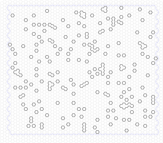
(a) $n=8$ and $x=0.5$. Theorem 1.6 shows that the limiting measure is unique for domains with vacant boundary conditions when $x$ is small.

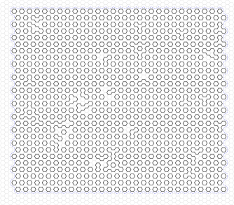
(b) $n=8$ and $x=2$. Theorem 1.8 shows that typical configurations are small perturbations of the ground state for large $n$ and $x$.

Figure 2. Two samples of random loop configurations with large $n$. Configurations are on a $60\times 45$ domain of type $0$ and are sampled via Glauber dynamics for 100 million iterations started from the empty configuration.

1.1. Results

In order to state our main results, we need several more definitions (see Figure 1 for their illustration). We consider the triangular lattice $\mathbb{T}:=(0,2)\mathbb{Z}+(\sqrt{3},1)\mathbb{Z}$, and view the hexagonal lattice $\mathbb{H}$ as its dual lattice, obtained by placing a vertex at the center of every face (triangle) of $\mathbb{T}$, so that each edge $e$ of $\mathbb{H}$ corresponds to the unique edge $e^{*}$ of $\mathbb{T}$ which intersects $e$. Since vertices of $\mathbb{T}$ are identified with faces of $\mathbb{H}$, they will be called hexagons instead of vertices. We will also say that a vertex or an edge of $\mathbb{H}$ borders a hexagon if it borders the corresponding face of $\mathbb{H}$.

There are exactly 6 proper colorings of $\mathbb{T}$ with the colors $\{0,1,2\}$. For the rest of the paper, we fix an arbitrary proper coloring and let $\mathbb{T}^{{\mathsf{c}}}$ be the set of hexagons colored by ${{\mathsf{c}}}$, ${{\mathsf{c}}}\in\{0,1,2\}$. A trivial loop is a loop of length exactly $6$. Define the ${{\mathsf{c}}}$-phase ground state $\omega_{\operatorname{gnd}}^{{\mathsf{c}}}$ to be the (fully-packed) loop configuration consisting of all the trivial loops surrounding hexagons in $\mathbb{T}^{{\mathsf{c}}}$. We shall say that a domain $H$ is of type ${{\mathsf{c}}}$, ${{\mathsf{c}}}\in\{0,1,2\}$, if every edge $\{u,v\}\in\omega_{\operatorname{gnd}}^{{\mathsf{c}}}$ satisfies either $u,v\in V(H)$ or $u,v\notin V(H)$. Equivalently, $H$ is of type ${{\mathsf{c}}}$ if and only if

$$\mathsf{LoopConf}(H,\emptyset)=\{\omega\cap E(H):\omega\in\mathsf{LoopConf}(H,\omega_{\operatorname{gnd}}^{{\mathsf{c}}})\}.$$ (3)

Finally, we shall say that a loop surrounds a vertex $u$ of $\mathbb{H}$ if any infinite simple path in $\mathbb{H}$ starting at $u$ intersects a vertex of this loop. In particular, if a loop passes through a vertex then it surrounds it as well.

Theorem 1.4.

There exist $n_{0},\alpha>0$ such that for any $n\geq n_{0}$ and $x\in(0,\infty]$ the following holds. For any ${{\mathsf{c}}}\in\{0,1,2\}$, any domain $H$ of type ${{\mathsf{c}}}$, any $u\in V(H)$ and any integer $k>6$, we have

$$\mathbb{P}_{H,n,x}^{\emptyset}(\text{there exists a loop of length $k$ surrounding $u$})\leq n^{-\alpha k}.$$

As follows from Theorem 1.8 below, when $n$ and $nx^{6}$ are sufficiently large, it is likely that $u$ is contained in a trivial loop. Thus, the assumption that $k>6$ is necessary. The techniques involved in the proof of Theorem 1.4 also imply the following result, which partially answers Question 1.2.

Theorem 1.5.

There exist $n_{0},\alpha>0$ such that for any $n\geq n_{0}$ and any $x>0$ the following holds. For any ${{\mathsf{c}}}\in\{0,1,2\}$, any domain $H$ of type ${{\mathsf{c}}}$ and any distinct non-adjacent $u,v\in V(H)$, we have

$$\frac{\displaystyle\sum_{\lambda\in\mathsf{LoopConf}(H,\emptyset,u,v)}x^{o_{H}(\lambda)}n^{L^{\prime}_{H}(\lambda)}J(\lambda)}{\displaystyle\sum_{\omega\in\mathsf{LoopConf}(H,\emptyset)}x^{o_{H}(\omega)}n^{L_{H}(\omega)}}\leq x\cdot n^{-\alpha\,d_{H}(u,v)},$$

where $d_{H}(u,v)$ is the graph distance in $H$ between $u$ and $v$.

Our techniques provide additional information on the (infinite-volume) Gibbs measures of the loop $O(n)$ model. We recall the standard definition: a probability measure $\mathbb{P}$ on the set of loop configurations on $\mathbb{H}$ (viewed as a subset of $\{0,1\}^{E(\mathbb{H})}$) is a Gibbs measure for the loop $O(n)$ model with edge weight $x$ if for any domain $H$ and $\mathbb{P}$-almost every loop configuration $\xi$, the distribution of the configuration $\omega$, conditioned that $\omega\in\mathsf{LoopConf}(H,\xi)$, is given by $\mathbb{P}^{\xi}_{H,n,x}$.

For small parameter $x$, under vacant boundary conditions, the model is in a dilute, disordered phase, where loops are rare and tend to be short; see Figure 2(a). This is relatively simple to show and is proved in Corollary 3.2. A consequence of this fact is the existence of a unique limiting Gibbs measure when exhausting the hexagonal lattice $\mathbb{H}$ via domains with vacant boundary conditions.

Theorem 1.6.

There exists $c>0$ such that for any $n>0$ and $0<x\leq c$ satisfying $nx^{6}\leq c$ the following holds. Let $H_{k}$ be an increasing sequence of domains satisfying $\cup_{k}H_{k}=\mathbb{H}$. Then the measures $\mathbb{P}_{H_{k},n,x}^{\emptyset}$ converge (weakly) as $k\to\infty$ to an infinite-volume Gibbs measure $\mathbb{P}_{\mathbb{H},n,x}$ which is supported on loop configurations with no infinite paths.

It follows that the limiting measure $\mathbb{P}_{\mathbb{H},n,x}$ does not depend on the specific choice of exhausting sequence $(H_{k})$ as one may interleave two such sequences to obtain another convergent sequence. Consequently, it also follows that $\mathbb{P}_{\mathbb{H},n,x}$ is invariant under automorphisms of $\mathbb{H}$. Our proofs apply also when one allows $H_{k}$ to be arbitrary finite subgraphs of $\mathbb{H}$ rather than domains, but we do not state this explicitly as our work is mostly concerned with domains. The restriction to vacant boundary conditions is, however, essential for our proofs with the difficulty stemming from the fact that non-vacant boundary conditions may force the existence of long paths in the configuration (see Figure 3(b)). Still, it may be that there is a unique Gibbs measure in this regime of small $x$ and we provide a discussion of this in Section 4.

For large parameter $x$ and large $n$, the situation changes dramatically. Here, we obtain that the model is in a dense, ordered phase, where, under the $\omega_{\operatorname{gnd}}^{{\mathsf{c}}}$ boundary conditions, a typical configuration is a perturbation of that ground state. As a consequence of this structure, the model has at least three different limiting Gibbs measures in this regime of $n$ and $x$. We state this precisely in the following theorem. To lighten the notation, we write $\mathbb{P}_{H,n,x}^{{\mathsf{c}}}$ for the loop $O(n)$ measure on $H$ with boundary conditions $\omega_{\operatorname{gnd}}^{{\mathsf{c}}}$.

Theorem 1.7.

There exists $C>0$ such that for any $n\geq C$ and any $x\in(0,\infty]$ satisfying $nx^{6}\geq C$ the following holds. Let $H_{k}$ be an increasing sequence of domains satisfying $\cup_{k}H_{k}=\mathbb{H}$. Then, for every ${{\mathsf{c}}}\in\{0,1,2\}$, the measures $\mathbb{P}_{H_{k},n,x}^{{{\mathsf{c}}}}$ converge (weakly) as $k\to\infty$ to an infinite-volume Gibbs measure $\mathbb{P}_{\mathbb{H},n,x}^{{\mathsf{c}}}$ which is supported on loop configurations with no infinite paths. Furthermore, no one of the limiting measures is a convex combination of the other two.

Similarly to before, it follows that, for each ${{\mathsf{c}}}\in\{0,1,2\}$, the limiting measure $\mathbb{P}_{\mathbb{H},n,x}^{{\mathsf{c}}}$ does not depend on the specific choice of exhausting sequence $(H_{k})$ and that $\mathbb{P}_{\mathbb{H},n,x}^{{\mathsf{c}}}$ is invariant under automorphisms preserving the set $\mathbb{T}^{{\mathsf{c}}}$. However, as these measures are distinct for different ${{\mathsf{c}}}$, they are not invariant under all automorphisms. In particular, if each $H_{k}$ is of type ${{\mathsf{c}}}$, by (3), we have that $\mathbb{P}_{H_{k},n,x}^{\emptyset}$ also converges to $\mathbb{P}_{\mathbb{H},n,x}^{{\mathsf{c}}}$, in contrast to the behavior obtained in Theorem 1.6 for small $x$. It would be interesting to determine whether every infinite-volume Gibbs measure is a convex combination of these three measures, i.e., whether these are the only extremal Gibbs measures (see also Section 4). As we remark at the end of the section, this is not the case for $x=\infty$.

As mentioned above, in the ordered regime (large $x$ and $n$), a typical configuration drawn from $\mathbb{P}_{H,n,x}^{{\mathsf{c}}}$ is a perturbation of the ${{\mathsf{c}}}$-phase ground state $\omega_{\operatorname{gnd}}^{{\mathsf{c}}}$ (see Figure 2(b)). This is made precise in the following theorem, which we state for the ${{\mathsf{c}}}=0$ phase for concreteness of our definitions. In order to measure how close $\omega_{\operatorname{gnd}}^{0}$ and a typical loop configuration are, we introduce the notion of a breakup. Fix a domain $H$ and let $\omega\in\mathsf{LoopConf}(H,\omega_{\operatorname{gnd}}^{0})$ be a loop configuration. Let $A(\omega)$ be the set of vertices of $\mathbb{H}$ belonging to trivial loops surrounding hexagons in $\mathbb{T}^{0}$ and let $B(\omega)$ be the unique infinite connected component of $A(\omega)$. For $u\in\mathbb{H}$, define the breakup ${{\mathcal{C}}}(\omega,u)$ of $u$ to be the connected component of $\mathbb{H}\setminus B(\omega)$ containing $u$, setting ${{\mathcal{C}}}(\omega,u)=\emptyset$ if $u\in B(\omega)$. We also define $\partial{{\mathcal{C}}}(\omega,u)$ to be the internal vertex boundary of ${{\mathcal{C}}}(\omega,u)$, i.e., the set of vertices in ${{\mathcal{C}}}(\omega,u)$ adjacent to a vertex not in ${{\mathcal{C}}}(\omega,u)$ (thus in $B(\omega)$). We remark that ${{\mathcal{C}}}(\omega,u)$ need not be contained in $H$, though it cannot extend significantly beyond it in the sense that it is contained in any domain of type $0$ containing $H$.

Theorem 1.8.

There exists $c>0$ such that for any $n>0$, any $x\in(0,\infty]$, any domain $H$, any $u\in V(H)$ and any positive integer $k$, we have

$$\mathbb{P}_{H,n,x}^{0}(|\partial{{\mathcal{C}}}(\omega,u)|\geq k)\leq(cn\cdot\min\{x^{6},1\})^{-k/15}.$$

One should note that the above theorem contains the implicit assumption that $n\geq C$ and $nx^{6}\geq C$, as otherwise the statement is trivial.

In this work, we mainly study the loop $O(n)$ model with either vacant or ground state boundary conditions. To obtain a complete picture regarding the possible Gibbs measures, one must also study the model for general boundary conditions. As mentioned above, understanding the Gibbs measures in each regime of $n$ and $x$, and in particular, determining the number of extremal Gibbs measures, is an interesting problem. Theorem 1.6 and Theorem 1.7 bring us closer to this goal, providing a partial answer in the regimes $nx^{6}\leq c$ and $nx^{6}\geq C$, for large $n$. In this regard, one may ask what happens in the intermediate regime, i.e., when $c<nx^{6}<C$ and $n$ is large. For instance, one may ask whether or not there is a single transition curve, perhaps of the form $nx^{6}=c^{\prime}$. If indeed this is the case, it would be interesting to investigate the number of extremal Gibbs measures on this curve, determining whether there is a unique such Gibbs measure (as Theorem 1.6 suggests for $nx^{6}\leq c$), $3$ such measures (as Theorem 1.7 suggests for $nx^{6}\geq C$), $4$ such measures, or perhaps a different quantity (see also Section 4).

Remark.

For $x=0$ and $x=\infty$, many other Gibbs measures can be constructed. For instance, for positive integers $a$ and $b$, let $H_{a,b}$ be the “rectangle” of width $2a+1$ and height $b$ (measured in hexagons) with the origin at the center, as in Figure 3(a) (on the left). It is not hard to check that the configuration depicted in the figure is the unique fully-packed loop configuration (with vacant boundary conditions) inside $H_{a,b}$. Thus, the probability measure $\mathbb{P}_{H_{a,b},n,\infty}^{\emptyset}$ is supported on a single configuration. The measures $\mathbb{P}_{H_{a,b},n,\infty}^{\emptyset}$ converge (as $a,b\to\infty$) to a delta measure on the configuration of infinite vertical paths covering the entire lattice (which is a Gibbs measure of the loop $O(n)$ model with edge weight $\infty$). By considering different domains, one may construct many more examples of this nature (once again, see Figure 3(a)). One may also look at the limiting model as $x$ tends to $0$, which corresponds to requiring the configuration to have the minimal number of edges. For the vacant boundary conditions, the finite-volume measure is a Dirac measure on the empty configuration. Using alternative boundary conditions, one may construct several distinct Gibbs measures (see, e.g., Figure 3(b)).

(a) Domains for which there exists a single fully-packed loop configuration (with vacant boundary conditions). Using such domains, one may obtain many weak limits of the probability measures $\mathbb{P}_{H,n,\infty}^{\emptyset}$.

(b) A domain with boundary conditions inducing a unique loop configuration with minimal number of edges. Such domains give rise to a Gibbs measure for $x=0$ which contains an infinite interface passing near the origin.

Figure 3. Constructing multiple Gibbs measures when $x=0$ or $x=\infty$ through suitable domains and boundary conditions.

1.2. Overview of the proof

Our proofs make use of the following simple lemma.

Lemma 1.9.

Let $p,q>0$ and let $E$ and $F$ be two events in a discrete probability space. If there exists a map $\mathsf{T}\colon E\to F$ such that $\mathbb{P}(\mathsf{T}(e))\geq p\cdot\mathbb{P}(e)$ for every $e\in E$, and $|\mathsf{T}^{-1}(f)|\leq q$ for every $f\in F$, then

$$\mathbb{P}(E)\leq\frac{q}{p}\cdot\mathbb{P}(F).$$

Proof.

We have

$$p\cdot\mathbb{P}(E)\leq\sum_{e\in E}\mathbb{P}(\mathsf{T}(e))=\sum_{e\in E}\sum_{f\in F}\mathbb{P}(f)\mathbf{1}_{\{\mathsf{T}(e)=f\}}=\sum_{f\in F}|\mathsf{T}^{-1}(f)|\cdot\mathbb{P}(f)\leq q\cdot\mathbb{P}(F).\qed$$

The results for small $x$ are obtained via a fairly standard, and short, Peierls argument, by applying the above lemma to a map which removes loops. For details, we refer the reader to Section 3.1. The main novelty of this work lies in the study of the loop $O(n)$ model for large $x$.

In the large $x$ regime, the idea is to apply the above lemma to a suitably defined ‘repair map’. This map takes a configuration $\omega$ sampled with $0$-phase ground state boundary conditions (or vacant boundary conditions in a domain of type $0$) and having a large breakup and returns a ‘repaired’ configuration in which the breakup is significantly reduced. The map operates by identifying regions in which the configuration resembles one of the three ground states. Regions resembling the $\omega_{\operatorname{gnd}}^{1}$ state are ‘shifted down’ by one hexagon to resemble $\omega_{\operatorname{gnd}}^{0}$ and similarly regions resembling $\omega_{\operatorname{gnd}}^{2}$ are ‘shifted up’ by one hexagon to resemble $\omega_{\operatorname{gnd}}^{0}$. Regions resembling the $\omega_{\operatorname{gnd}}^{0}$ state are left untouched. Regions which do not resemble any of the ground states are completely replaced by trivial loops from the $\omega_{\operatorname{gnd}}^{0}$ state. We show that this yields a new loop configuration, compatible with the boundary conditions, and having much higher probability. To finish using Lemma 1.9, we further show that the number of preimages of a given loop configuration is exponentially smaller than the probability gain. This yields the main lemma of our paper, Lemma 2.10, from which our results for large $x$ are later deduced. The repair map is illustrated in Figure LABEL:fig:proof-illustration and is formally defined in Section 2.3 following the definitions of ‘flowers’, ‘gardens’ and ‘clusters’ which we require to make precise the notion of resembling a ground state.

1.3. Graph notation

Throughout this paper, given a graph $G$, we shall denote its vertex and edge sets by $V(G)$ and $E(G)$, respectively. If $u,v\in V(G)$ are such that $\{u,v\}\in E(G)$, we say that $u$ and $v$ are adjacent (or neighbors) in $G$ and we drop the dependence on $G$ if it is clear from the context. For a vertex $u$ and an edge $e$ such that $u\in e$, we say that $e$ is incident to $u$ and that $u$ is an endpoint of $e$. For $A\subset V(G)$, we define its (vertex) boundary $\partial A$ by

$$\partial A:=\big{\{}u\in A\leavevmode\nobreak\ :\leavevmode\nobreak\ \{u,v\}\in E(G)\text{ for some }v\not\in A\big{\}}.$$

The following is a standard lemma which gives a bound on the number of connected induced subgraphs of a graph.

Lemma 1.10 ([5, Chapter 45]).

Let $G$ be a graph with maximum degree $d\geq 3$. The number of connected subsets of $V(G)$ containing a given vertex and $k$ other vertices is at most $(e(d-1))^{k}$.

1.4. Organization of the article

The rest of the article is structured as follows. Section 2 introduces the repair map and proves the main lemma, Lemma 2.10. In Section 3, we derive our theorems. The statements regarding large $x$ are deduced from the main lemma whereas the parts pertaining to small $x$, being simpler, are obtained directly. In Section 4, we discuss several directions for future research.

1.5. Acknowledgements

We are grateful to two anonymous referees whose comments helped to improve the exposition and elucidate the relation of the results with the existing literature.

2. Flowers, gardens and the repair map

This section is devoted to the formulation and proof of the main lemma, Lemma 2.10. We start by stating a few definitions in Section 2.1. In particular, we introduce the notions of a circuit, ${{\mathsf{c}}}$-flower, ${{\mathsf{c}}}$-garden and ${{\mathsf{c}}}$-cluster, and gather some easy general facts about these objects. The main lemma is stated in Section 2.2 and the remaining sections are devoted to its proof. Section 2.3 introduces the repair map, which will play the role of $\mathsf{T}$ in Lemma 1.9. Section 2.4 compares the probability of a configuration and its image under the repair map (which corresponds to estimating $p$ in Lemma 1.9). Section 2.5 gathers the last ingredients (mainly an estimate for the number of possible preimages under the repair map, which corresponds to bounding $q$ in Lemma 1.9) to conclude the proof of Lemma 2.10.

2.1. Definitions and gardening

A circuit is a simple closed path in $\mathbb{T}$, which may be viewed as a sequence of hexagons $\gamma=(\gamma_{0},\dots,\gamma_{m})$, $m\geq 3$, satisfying the following two properties:

• $\gamma_{m}=\gamma_{0}$ and $\gamma_{i}\neq\gamma_{j}$ for every $0\leq i<j<m$,

• $\gamma_{i}$ and $\gamma_{i+1}$ are neighbors (in $\mathbb{T}$) for every $0\leq i<m$.

Define $\gamma^{*}$ to be the set of edges $\{\gamma_{i},\gamma_{i+1}\}^{*}\in E(\mathbb{H})$ for $0\leq i<m$.

We proceed with three standard geometric facts regarding circuits and domains. For completeness, these facts are proved in Appendix B. The first two facts constitute a discrete version of the Jordan curve theorem.

Fact 2.1.

If $\gamma$ is a circuit then the removal of $\gamma^{*}$ splits $\mathbb{H}$ into exactly two connected components, one of which is infinite, denoted by $\mathrm{Ext}(\gamma)$, and one of which is finite, denoted by $\mathrm{Int}(\gamma)$. Moreover, each of these are induced subgraphs of $\mathbb{H}$.

Let $\gamma$ be a circuit. We denote the vertex sets and edge sets of $\mathrm{Int}(\gamma),\mathrm{Ext}(\gamma)$ by $\mathrm{Int}^{\mathrm{V}}(\gamma),\mathrm{Ext}^{\mathrm{V}}(\gamma)$ and $\mathrm{Int}^{\mathrm{E}}(\gamma),\mathrm{Ext}^{\mathrm{E}}(\gamma)$, respectively. Note that $\{\mathrm{Int}^{\mathrm{V}}(\gamma),\mathrm{Ext}^{\mathrm{V}}(\gamma)\}$ is a partition of $V(\mathbb{H})$ and that $\{\mathrm{Int}^{\mathrm{E}}(\gamma),\mathrm{Ext}^{\mathrm{E}}(\gamma),\gamma^{*}\}$ is a partition of $E(\mathbb{H})$. We also define $\mathrm{Int}^{\mathrm{hex}}(\gamma)$ to be the set of faces of $\mathrm{Int}(\gamma)$, i.e., the set of hexagons $z\in\mathbb{T}$ having all their six bordering vertices in $\mathrm{Int}^{\mathrm{V}}(\gamma)$. Since $\mathrm{Int}(\gamma)$ is induced, this is equivalent to having all six bordering edges in $\mathrm{Int}^{\mathrm{E}}(\gamma)$.

Note that, by Fact 2.1, $\mathrm{Int}(\gamma)$ is a domain. The converse is also true.

Fact 2.2.

Circuits are in one-to-one correspondence with domains via $\gamma\leftrightarrow\mathrm{Int}(\gamma)$.

Hence, every domain $H$ may be written as $H=\mathrm{Int}(\gamma)$ for some circuit $\gamma$. Recalling the definition from Section 1.1 of a domain of type ${{\mathsf{c}}}\in\{0,1,2\}$, one should also note that $H$ is of type ${{\mathsf{c}}}$ if and only if $\gamma\subset\mathbb{T}\setminus\mathbb{T}^{{\mathsf{c}}}$.

Fact 2.3.

Let $\sigma$ and $\sigma^{\prime}$ be two circuits such that $\sigma^{*}\cap(\sigma^{\prime})^{*}\neq\emptyset$ or $\mathrm{Int}^{\mathrm{V}}(\sigma)\cap\mathrm{Int}^{\mathrm{V}}(\sigma^{\prime})\neq\emptyset$. Then there exists a circuit $\gamma\subset\sigma\cup\sigma^{\prime}$ such that $\gamma^{*}\subset\sigma^{*}\cup(\sigma^{\prime})^{*}$ and $\mathrm{Int}(\sigma)\cup\mathrm{Int}(\sigma^{\prime})\subset\mathrm{Int}(\gamma)$.

Figure 4. A garden. The dashed line denotes a vacant circuit $\sigma\subset\mathbb{T}\setminus\mathbb{T}^{{\mathsf{c}}}$, where ${{\mathsf{c}}}\in\{0,1,2\}$. The edges inside $\sigma$, along with the edges crossing $\sigma$, then comprise a ${{\mathsf{c}}}$-garden of $\omega$, since every hexagon in $\mathbb{T}^{{\mathsf{c}}}\cap\partial\mathrm{Int}^{\mathrm{hex}}(\sigma)$ is surrounded by a trivial loop.

Definition 2.4 (${{\mathsf{c}}}$-flower, ${{\mathsf{c}}}$-garden, vacant circuit; see Figure 4).

Let ${{\mathsf{c}}}\in\{0,1,2\}$ and let $\omega$ be a loop configuration. A hexagon $z\in\mathbb{T}^{{\mathsf{c}}}$ is a ${{\mathsf{c}}}$-flower of $\omega$ if it is surrounded by a trivial loop in $\omega$. A subset $E\subset E(\mathbb{H})$ is a ${{\mathsf{c}}}$-garden of $\omega$ if there exists a circuit $\sigma\subset\mathbb{T}\setminus\mathbb{T}^{{\mathsf{c}}}$ such that $E=\mathrm{Int}^{\mathrm{E}}(\sigma)\cup\sigma^{*}$ and every $z\in\mathbb{T}^{{\mathsf{c}}}\cap\partial\mathrm{Int}^{\mathrm{hex}}(\sigma)$ is a ${{\mathsf{c}}}$-flower of $\omega$. In this case, we denote $\sigma(E):=\sigma$. A circuit $\sigma$ is vacant in $\omega$ if $\omega\cap\sigma^{*}=\emptyset$.

We say that $E\subset E(\mathbb{H})$ is a garden of $\omega$ if it is a ${{\mathsf{c}}}$-garden of $\omega$ for some ${{\mathsf{c}}}\in\{0,1,2\}$. We stress the fact that a garden is a subset of the edges of $\mathbb{H}$. We continue with several simple properties of circuits, gardens and loop configurations which will be used throughout the paper.

Lemma 2.5.

Let $\omega$ and $\omega^{\prime}$ be two loop configurations.

1. If $\sigma$ is a vacant circuit in $\omega$ then $\omega\cap\mathrm{Int}^{\mathrm{E}}(\sigma)$ and $\omega\cap\mathrm{Ext}^{\mathrm{E}}(\sigma)$ are loop configurations.

2. If $E$ is a garden of $\omega$ then $\sigma(E)$ is a vacant circuit in $\omega$.

3. If $E$ is a garden of $\omega$ then $\omega\cap E$ and $\omega\setminus E$ are loop configurations.

4. If $\omega$ and $\omega^{\prime}$ are disjoint then $\omega\cup\omega^{\prime}$ is a loop configuration.

5. If $\omega^{\prime}$ is contained in $\omega$ then $\omega\setminus\omega^{\prime}$ is a loop configuration.

Proof.

To see (a), let $\sigma$ be a vacant circuit in $\omega$. Since any path between $\mathrm{Int}(\sigma)$ and $\mathrm{Ext}(\sigma)$ intersects $\sigma^{*}$, and since $\omega\cap\sigma^{*}=\emptyset$, every loop of $\omega$ is contained in either $\mathrm{Int}(\sigma)$ or $\mathrm{Ext}(\sigma)$, and thus, (a) follows.

We now show (b). Let $E$ be a ${{\mathsf{c}}}$-garden of $\omega$, ${{\mathsf{c}}}\in\{0,1,2\}$, and let $\sigma:=\sigma(E)$. One of the endpoints of every edge $e\in\sigma^{*}$ must border a hexagon in $\mathbb{T}^{{\mathsf{c}}}\cap\partial\mathrm{Int}^{\mathrm{hex}}(\sigma)$. By the definition of a ${{\mathsf{c}}}$-garden, this hexagon is a ${{\mathsf{c}}}$-flower, and hence, $e$ cannot belong to $\omega$. Thus, $\sigma$ is vacant in $\omega$.

In light of (a) and (b), (c) is immediate.

To establish (d), it suffices to show that no vertex has degree $3$ in $\omega^{\prime}\cup\omega$. Indeed, if a vertex has degree $3$ then one of the edges incident to it must be contained in both $\omega$ and $\omega^{\prime}$, which is a contradiction.

Finally, the last statement is straightforward. ∎

Lemma 2.6.

Let ${{\mathsf{c}}}\in\{0,1,2\}$, let $\sigma\subset\mathbb{T}\setminus\mathbb{T}^{{\mathsf{c}}}$ be a circuit, let $z\in\mathbb{T}^{{\mathsf{c}}}$ be a hexagon and let $V(z)$ denote the six vertices in $\mathbb{H}$ bordering $z$. Then

$$z\in\mathrm{Int}^{\mathrm{hex}}(\sigma)\quad\iff\quad V(z)\cap\mathrm{Int}^{\mathrm{V}}(\sigma)\neq\emptyset.$$

Proof.

Recall that, by definition, $z\in\mathrm{Int}^{\mathrm{hex}}(\sigma)$ if and only if $V(z)\subset\mathrm{Int}^{\mathrm{V}}(\sigma)$. Thus, it suffices to check that if $v\in V(z)\cap\mathrm{Int}^{\mathrm{V}}(\sigma)$ and $u\in V(z)$ is adjacent to $v$ then $u\in\mathrm{Int}^{\mathrm{V}}(\sigma)$. Indeed this is the case, as otherwise, $\{u,v\}\in\sigma^{*}$ and $z\in\sigma$, which contradicts the assumption that $\sigma\subset\mathbb{T}\setminus\mathbb{T}^{{\mathsf{c}}}$. ∎

We proceed to discuss disjointness and containment properties of gardens.

Lemma 2.7.

Let $\omega$ be a loop configuration and let $E_{1}$ and $E_{2}$ be two ${{\mathsf{c}}}$-gardens of $\omega$ for some ${{\mathsf{c}}}\in\{0,1,2\}$. If there exists a vertex which is the endpoint of an edge in $E_{1}$ and an edge in $E_{2}$, then $E_{1}\cup E_{2}$ is contained in a ${{\mathsf{c}}}$-garden of $\omega$.

Proof.

Denote $\sigma_{1}:=\sigma(E_{1})$ and $\sigma_{2}:=\sigma(E_{2})$. Let us first show that necessarily $\mathrm{Int}^{\mathrm{V}}(\sigma_{1})\cap\mathrm{Int}^{\mathrm{V}}(\sigma_{2})\neq\emptyset$ or $\sigma_{1}^{*}\cap\sigma_{2}^{*}\neq\emptyset$. To this end, let $v,u,w\in V(\mathbb{H})$ be such that $\{v,u\}\in E_{1}$ and $\{v,w\}\in E_{2}$. If $v\in\mathrm{Int}^{\mathrm{V}}(\sigma_{1})\cap\mathrm{Int}^{\mathrm{V}}(\sigma_{2})$ then we are done. Otherwise, suppose without loss of generality that $v\in\mathrm{Ext}^{\mathrm{V}}(\sigma_{1})$ so that $u\in\mathrm{Int}^{\mathrm{V}}(\sigma_{1})$. If also $v\in\mathrm{Ext}^{\mathrm{V}}(\sigma_{2})$ then necessarily $w=u$ and $w\in\mathrm{Int}^{\mathrm{V}}(\sigma_{2})$ as $\sigma_{1},\sigma_{2}\subset\mathbb{T}\setminus\mathbb{T}^{{\mathsf{c}}}$. If instead $v\in\mathrm{Int}^{\mathrm{V}}(\sigma_{2})$ then either $u\in\mathrm{Int}^{\mathrm{V}}(\sigma_{2})$ or $\{v,u\}\in\sigma_{1}^{*}\cap\sigma_{2}^{*}$.

By Fact 2.3, there exists a circuit $\gamma$ such that $\gamma^{*}\subset\sigma_{1}^{*}\cup\sigma_{2}^{*}$ and $\mathrm{Int}(\sigma_{1})\cup\mathrm{Int}(\sigma_{2})\subset\mathrm{Int}(\gamma)$. In particular, $E_{1}\cup E_{2}\subset E$, where $E:=\mathrm{Int}^{\mathrm{E}}(\gamma)\cup\gamma^{*}$. It remains to show that $E$ is a ${{\mathsf{c}}}$-garden of $\omega$. Since, by Lemma 2.6, $\mathbb{T}^{{\mathsf{c}}}\cap\partial\mathrm{Int}^{\mathrm{hex}}(\gamma)\subset\partial\mathrm{Int}^{\mathrm{hex}}(\sigma_{1})\cup\partial\mathrm{Int}^{\mathrm{hex}}(\sigma_{2})$, this follows from the assumption that $E_{1}$ and $E_{2}$ are ${{\mathsf{c}}}$-gardens of $\omega$. ∎

Lemma 2.8.

Let $\omega$ be a loop configuration, let $E_{0}$ be a ${{\mathsf{c}}}_{0}$-garden of $\omega$ and let $E_{1}$ be a ${{\mathsf{c}}}_{1}$-garden of $\omega$ with ${{\mathsf{c}}}_{0},{{\mathsf{c}}}_{1}\in\{0,1,2\}$ distinct. Then, either $E_{0}\subset E_{1}$, $E_{1}\subset E_{0}$ or $E_{0}\cap E_{1}=\emptyset$.

Proof.

Assume without loss of generality that ${{\mathsf{c}}}_{0}=0$, ${{\mathsf{c}}}_{1}=1$ and that $E_{0}\cap E_{1}\neq\emptyset$. Denote $\sigma_{0}:=\sigma(E_{0})\subset\mathbb{T}\setminus\mathbb{T}^{0}$ and $\sigma_{1}:=\sigma(E_{1})\subset\mathbb{T}\setminus\mathbb{T}^{1}$. Consider an infinite path in $\mathbb{H}$ beginning with some edge of $E_{0}\cap E_{1}$ and let $e\in E(\mathbb{H})$ be the first edge on this path that is not in $\mathrm{Int}^{\mathrm{E}}(\sigma_{0})\cap\mathrm{Int}^{\mathrm{E}}(\sigma_{1})$ (maybe the first edge itself). We may assume without loss of generality that $e\notin\mathrm{Int}^{\mathrm{E}}(\sigma_{0})$. Thus, $e\in\sigma_{0}^{*}$, and, therefore, $e$ is bordered by a hexagon $z\in\mathbb{T}^{1}$ and a hexagon in $\mathbb{T}^{2}$. Since $e$ is also in $E_{1}$, $z$ belongs to $\mathrm{Int}^{\mathrm{hex}}(\sigma_{1})$, by Lemma 2.6. Now, if $\sigma_{0}\subset\mathrm{Int}^{\mathrm{hex}}(\sigma_{1})$ then $E_{0}\subset E_{1}$, by Fact 2.1. Otherwise, there exists $\{y,y^{\prime}\}\in\sigma_{0}^{*}$ such that $y\in\mathrm{Int}^{\mathrm{hex}}(\sigma_{1})$ and $y^{\prime}\notin\mathrm{Int}^{\mathrm{hex}}(\sigma_{1})$. In particular, $y^{\prime}$ must be in $\sigma_{0}\cap\sigma_{1}\subset\mathbb{T}^{2}$, so that $y$ must be in $\mathbb{T}^{1}$. Since $y$ is in $\partial\mathrm{Int}^{\mathrm{hex}}(\sigma_{1})$, it must be a $1$-flower of $\omega$. But since $y$ is on $\sigma_{0}$, it must also be adjacent to a $0$-flower of $\omega$, which is a contradiction. ∎

Definition 2.9 (${{\mathsf{c}}}$-cluster, ${{\mathsf{c}}}$-cluster inside $\gamma$).

Let ${{\mathsf{c}}}\in\{0,1,2\}$ and let $\omega$ be a loop configuration. A subset $E\subset E(\mathbb{H})$ is a ${{\mathsf{c}}}$-cluster of $\omega$ if it is a ${{\mathsf{c}}}$-garden of $\omega$ and it is not contained in any other garden of $\omega$. Let $\gamma$ be a vacant circuit in $\omega$ and note that $\omega\cap\mathrm{Int}^{\mathrm{E}}(\gamma)$ is a loop configuration by Lemma 2.5a. A subset $E\subset E(\mathbb{H})$ is a ${{\mathsf{c}}}$-cluster of $\omega$ inside $\gamma$ if it is a ${{\mathsf{c}}}$-cluster of $\omega\cap\mathrm{Int}^{\mathrm{E}}(\gamma)$.

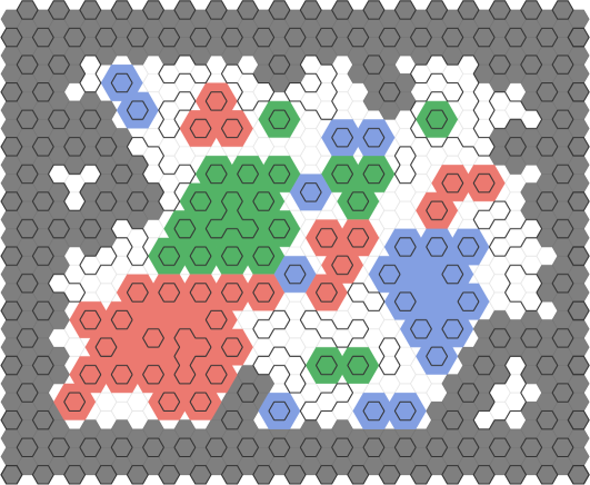
Figure 5. A loop configuration $\omega\in\mathsf{LoopConf}(H,\omega_{\operatorname{gnd}}^{0})$. The $0$-clusters are denoted in green, the $1$-clusters in red and the $2$-clusters in blue; all taken with respect to the circuit surrounding the large unshaded domain.

We say that $E\subset E(\mathbb{H})$ is a cluster (inside $\gamma$) if it is a ${{\mathsf{c}}}$-cluster (inside $\gamma$) for some ${{\mathsf{c}}}\in\{0,1,2\}$. Once again, note that a cluster (inside $\gamma$) is a subset of edges of $\mathbb{H}$. Evidently, a cluster of $\omega$ inside $\gamma$ is also a garden of $\omega$, but it is not necessarily a cluster of $\omega$. The notion of ${{\mathsf{c}}}$-cluster inside $\gamma$ will be important in the definition of the repair map in Section 2.3. Note that, by Lemma 2.7 and Lemma 2.8,

$$\text{any two distinct clusters of $\omega$ (inside $\gamma$) are edge disjoint},$$ (4)

and, moreover, for any ${{\mathsf{c}}}\in\{0,1,2\}$,

$$\text{the union of any two distinct ${{\mathsf{c}}}$-clusters of $\omega$ (inside $\gamma$) is a disconnected set of edges},$$ (5)

where a set of edges $E$ is said to be connected if the graph whose vertex set is the set of endpoints of edges in $E$ and whose edge set is $E$ is connected. Note also, that by Fact 2.1,

$$\text{every cluster of $\omega$ (inside $\gamma$) is a connected set of edges}.$$ (6)

2.2. Statement of the main lemma

We are now in a position to state the main lemma. For a loop configuration $\omega$ and a vacant circuit $\gamma$ in $\omega$, denote by $V(\omega,\gamma)$ the set of vertices $v\in\mathrm{Int}^{\mathrm{V}}(\gamma)$ such that the three edges of $\mathbb{H}$ incident to $v$ are not all contained in the same cluster of $\omega$ inside $\gamma$. One checks simply using Lemma 2.6 that a vertex $v\in\mathrm{Int}^{\mathrm{V}}(\gamma)$ satisfies $v\in V(\omega,\gamma)$ if and only if $v$ is incident to an edge which is not in any cluster or each of its incident edges lies in a different cluster.

For a vacant circuit $\gamma\subset\mathbb{T}\setminus\mathbb{T}^{0}$, the set $V(\omega,\gamma)$ specifies the deviation in $\omega$ from the $0$-phase ground state along the interior boundary of $\gamma$. Our main lemma shows that having a large deviation is exponentially unlikely.

Lemma 2.10.

There exists an absolute constant $c>0$ such that for any $n>0$, any $x\in(0,\infty]$, any domain $H$, any circuit $\gamma\subset\mathbb{T}\setminus\mathbb{T}^{0}$ and any positive integer $k$, we have

$$\mathbb{P}_{H,n,x}^{0}\big{(}\partial\mathrm{Int}^{\mathrm{V}}(\gamma)\subset V(\omega,\gamma)\text{ and }|V(\omega,\gamma)|\geq k\,\mid\,\text{$\gamma$ vacant}\big{)}\leq(cn\cdot\min\{x^{6},1\})^{-k/15}.$$

The reader should first have in mind the simpler case of the lemma in which $H=\mathrm{Int}(\gamma)$. In this case the boundary conditions may equivalently be taken to be vacant. The lemma is stated in greater generality, allowing, in particular, for $\gamma$ to leave the domain $H$, i.e., for $\mathrm{Int}(\gamma)\not\subset H$. This additional flexibility is used in the proofs of Theorem 1.7 and Theorem 1.8 to handle the case of domains without a type.

One should note that Lemma 2.10 contains the implicit assumption that $n\geq n\cdot\min\{x^{6},1\}\geq C$, as otherwise its statement is trivial.

2.3. Definition of the repair map

For the remainder of this section, we fix a circuit $\gamma\subset\mathbb{T}\setminus\mathbb{T}^{0}$ and set $H:=\mathrm{Int}(\gamma)$. Consider a loop configuration $\omega$ such that $\gamma$ is vacant in $\omega$. The idea of the repair map is to modify $\omega$ as follows:

• Edges in $1$-clusters inside $\gamma$ are shifted down “into the $0$-phase”.

• Edges in $2$-clusters inside $\gamma$ are shifted up “into the $0$-phase”.

• Edges in $0$-clusters inside $\gamma$ are left untouched.

• The remaining edges which are not inside (the shifted) clusters, but are in the interior of $\gamma$ (these edges will be called bad), are overwritten to “match” the $0$-phase ground state, $\omega_{\operatorname{gnd}}^{0}$.

See Figure LABEL:fig:proof-illustration for an illustration of this map.

In order to formalize this idea, we need a few definitions. A shift is a graph automorphism of $\mathbb{T}$ which maps every hexagon to one of its neighbors. We henceforth fix a shift $\,\uparrow\,$ which maps $\mathbb{T}^{0}$ to $\mathbb{T}^{1}$ (and hence, maps $\mathbb{T}^{1}$ to $\mathbb{T}^{2}$ and $\mathbb{T}^{2}$ to $\mathbb{T}^{0}$), and denote its inverse by $\,\downarrow\,$. A shift naturally induces mappings on the set of vertices and the set of edges of $\mathbb{H}$. We shall use the same symbols, $\,\uparrow\,$ and $\,\downarrow\,$, to denote these mappings. Recall from Section 1.1 that $\mathbb{T}$ has a coordinate system given by $(0,2)\mathbb{Z}+(\sqrt{3},1)\mathbb{Z}$ and that $(\mathbb{T}^{0},\mathbb{T}^{1},\mathbb{T}^{2})$ are the color classes of an arbitrary proper $3$-coloring of $\mathbb{T}$. In our figures we make the choice that $(0,0)\in\mathbb{T}^{0}$ and $(0,2)\in\mathbb{T}^{1}$ so that $\,\uparrow\,$ is the map $(a,b)\mapsto(a,b+2)$.

For a loop configuration $\omega\in\mathsf{LoopConf}(H,\emptyset)$ and ${{\mathsf{c}}}\in\{0,1,2\}$, let $E^{{\mathsf{c}}}(\omega)\subset E(\mathbb{H})$ be the union of all ${{\mathsf{c}}}$-clusters of $\omega$. Note that, since $H=\mathrm{Int}(\gamma)$, for $\omega\in\mathsf{LoopConf}(H,\emptyset)$, the notions of a ${{\mathsf{c}}}$-cluster and a ${{\mathsf{c}}}$-cluster inside $\gamma$ coincide. For $\omega\in\mathsf{LoopConf}(H,\emptyset)$, define also

$$E^{\operatorname{bad}}(\omega) :=(\mathrm{Int}^{\mathrm{E}}(\gamma)\cup\gamma^{*})\setminus\big{(}E^{0}(\omega)\cup E^{1}(\omega)^{\,\downarrow\,}\cup E^{2}(\omega)^{\,\uparrow\,}\big{)},$$ (7)

$$\overline{E}(\omega) :=(\mathrm{Int}^{\mathrm{E}}(\gamma)\cup\gamma^{*})\setminus\big{(}E^{0}(\omega)\cup E^{1}(\omega)\cup E^{2}(\omega)\big{)}.$$ (8)

Note that, by (4), $\{E^{0}(\omega),E^{1}(\omega),E^{2}(\omega),\overline{E}(\omega)\}$ is a partition of $\mathrm{Int}^{\mathrm{E}}(\gamma)\cup\gamma^{*}$. Thus, Lemma 2.5 implies that

$$\omega\cap E^{0}(\omega) \omega\cap E^{1}(\omega) \omega\cap E^{2}(\omega) \omega\cap\overline{E}(\omega)$$, , and are pairwise disjoint loop configurations. (9)

See Figure 5 and Figure LABEL:fig:proof-illustration for an illustration of these notions. Finally, we define the repair map

$$R_{\gamma}\colon\mathsf{LoopConf}(H,\emptyset)\to\mathsf{LoopConf}(H,\emptyset)$$

by

$${R_{\gamma}(\omega)}:=\big{(}\omega\cap E^{0}(\omega)\big{)}\cup\big{(}\omega\cap E^{1}(\omega)\big{)}^{\,\downarrow\,}\cup\big{(}\omega\cap E^{2}(\omega)\big{)}^{\,\uparrow\,}\cup\big{(}\omega_{\operatorname{gnd}}^{0}\cap E^{\operatorname{bad}}(\omega)\big{)}.$$

The fact that the mapping is well-defined, i.e., that ${R_{\gamma}(\omega)}$ is indeed in $\mathsf{LoopConf}(H,\emptyset)$, is not completely straightforward. This follows from the following proposition, together with the simple property in Lemma 2.5d.

Proposition 2.11.

Let $\omega\in\mathsf{LoopConf}(H,\emptyset)$. Then $\omega\cap E^{0}(\omega)$, $(\omega\cap E^{1}(\omega))^{\,\downarrow\,}\cup(\omega\cap E^{2}(\omega))^{\,\uparrow\,}$ and $\omega_{\operatorname{gnd}}^{0}\cap E^{\operatorname{bad}}(\omega)$ are pairwise disjoint loop configurations in $\mathsf{LoopConf}(H,\emptyset)$.

We require the following simple geometric lemma.

Lemma 2.12.

Let $\sigma\subset\mathbb{T}\setminus\mathbb{T}^{0}$ and $\sigma^{\prime}\subset\mathbb{T}\setminus\mathbb{T}^{1}$ be circuits.

1. If $\mathrm{Int}(\sigma^{\prime})\subset\mathrm{Int}(\sigma)$ then $\mathrm{Int}(\sigma^{\prime})^{\,\downarrow\,}\subset\mathrm{Int}(\sigma)$.

2. If $\mathrm{Int}(\sigma^{\prime})\subset\mathrm{Ext}(\sigma)$ then $\mathrm{Int}(\sigma^{\prime})^{\,\downarrow\,}\subset\mathrm{Ext}(\sigma)$.

3. If $\mathrm{Int}^{\mathrm{V}}(\sigma^{\prime})\cap\mathrm{Int}^{\mathrm{V}}(\sigma)=\emptyset$ then $\mathrm{Int}^{\mathrm{V}}(\sigma^{\prime})^{\,\downarrow\,}\cap\mathrm{Int}^{\mathrm{V}}(\sigma)=\emptyset$.

Proof.

We first prove (a). The assumption that $\mathrm{Int}(\sigma^{\prime})\subset\mathrm{Int}(\sigma)$ implies that $\mathrm{Int}^{\mathrm{hex}}(\sigma^{\prime})\subset\mathrm{Int}^{\mathrm{hex}}(\sigma)$. By Lemma 2.6, any vertex $v$ in $\mathrm{Int}^{\mathrm{V}}(\sigma^{\prime})$ borders a hexagon in $\mathrm{Int}^{\mathrm{hex}}(\sigma^{\prime})$. Thus, it suffices to show that $\mathrm{Int}^{\mathrm{hex}}(\sigma^{\prime})^{\,\downarrow\,}\subset\mathrm{Int}^{\mathrm{hex}}(\sigma)$. Assume towards a contradiction that there exists a hexagon $z\in\mathrm{Int}^{\mathrm{hex}}(\sigma^{\prime})$ such that $z^{\,\downarrow\,}\notin\mathrm{Int}^{\mathrm{hex}}(\sigma)$. In such case, by Fact 2.1, $z^{\,\downarrow\,}$ must be in $\sigma\cap\sigma^{\prime}\subset\mathbb{T}^{2}$, and consequently, $z\in\mathbb{T}^{0}$. Therefore, as $z\in\mathrm{Int}^{\mathrm{hex}}(\sigma^{\prime})$ and $\sigma^{\prime}\subset\mathbb{T}\setminus\mathbb{T}^{1}$, Lemma 2.6 implies that the three neighbors of $z$ in $\mathbb{T}^{1}$ belong to $\mathrm{Int}^{\mathrm{hex}}(\sigma^{\prime})\subset\mathrm{Int}^{\mathrm{hex}}(\sigma)$. Now, Lemma 2.6 implies that $z^{\,\downarrow\,}$ has three neighbors in $\mathbb{T}^{0}\cap\mathrm{Int}^{\mathrm{hex}}(\sigma)$. In particular, the six vertices bordering $z^{\,\downarrow\,}$ belong to $\mathrm{Int}^{\mathrm{V}}(\sigma)$, implying that $z^{\,\downarrow\,}\in\mathrm{Int}^{\mathrm{hex}}(\sigma)$, which is a contradiction.

The proof of (b) is very similar to that of (a) and so we omit it.

Finally, by Fact 2.1, (c) is equivalent to (b). ∎

Proof of Proposition 2.11.

For the sake of brevity, throughout the proof, we drop $\omega$ from the notation of the above sets and write $E^{\operatorname{bad}}$, $E^{0}$, $E^{1}$ and $E^{2}$.

Step 1: $\omega\cap E^{0}$, $(\omega\cap E^{1})^{\,\downarrow\,}\cup(\omega\cap E^{2})^{\,\uparrow\,}$ and $\omega_{\operatorname{gnd}}^{0}\cap E^{\operatorname{bad}}$ are contained in $\mathrm{Int}^{\mathrm{E}}(\gamma)$.

Since $\gamma$ is vacant in both $\omega$ and $\omega_{\operatorname{gnd}}^{0}$, it follows that $\omega\cap E^{0}$ and $\omega_{\operatorname{gnd}}^{0}\cap E^{\operatorname{bad}}$ are contained in $\mathrm{Int}^{\mathrm{E}}(\gamma)$. It remains to show that $(\omega\cap E^{1})^{\,\downarrow\,}$ and $(\omega\cap E^{2})^{\,\uparrow\,}$ are contained in $\mathrm{Int}^{\mathrm{E}}(\gamma)$. We show this only for $(\omega\cap E^{1})^{\,\downarrow\,}$, as the other case is symmetric. Let $E$ be a $1$-cluster of $\omega$. We must show that $(\omega\cap E)^{\,\downarrow\,}\subset\mathrm{Int}^{\mathrm{E}}(\gamma)$. Since, by Lemma 2.5b, $\omega\cap E\subset\mathrm{Int}^{\mathrm{E}}(\sigma(E))\subset\mathrm{Int}^{\mathrm{E}}(\gamma)$, this follows from Lemma 2.12a.

Step 2: $\omega\cap E^{0}$, $(\omega\cap E^{1})^{\,\downarrow\,}\cup(\omega\cap E^{2})^{\,\uparrow\,}$ and $\omega_{\operatorname{gnd}}^{0}\cap E^{\operatorname{bad}}$ are pairwise disjoint.

By definition, $E^{\operatorname{bad}}$ (and therefore $\omega_{\operatorname{gnd}}^{0}\cap E^{\operatorname{bad}}$) is disjoint from the first two sets. It remains to show that $\omega\cap E^{0}$ is disjoint from $(\omega\cap E^{1})^{\,\downarrow\,}$ and $(\omega\cap E^{2})^{\,\uparrow\,}$. We show this only for $\omega\cap E^{0}$ and $(\omega\cap E^{1})^{\,\downarrow\,}$, as the other case is symmetric. Let $E$ and $E^{\prime}$ be $0$- and $1$-clusters of $\omega$, respectively. We must show that $(\omega\cap E)\cap(\omega\cap E^{\prime})^{\,\downarrow\,}=\emptyset$. By Lemma 2.5b, $(\omega\cap E)\cap(\omega\cap E^{\prime})^{\,\downarrow\,}\subset\mathrm{Int}^{\mathrm{E}}(\sigma(E))\cap\mathrm{Int}^{\mathrm{E}}(\sigma(E^{\prime}))^{\,\downarrow\,}$, which is empty by (4) and Lemma 2.12c.

Step 3: $\omega\cap E^{0}$, $(\omega\cap E^{1})^{\,\downarrow\,}\cup(\omega\cap E^{2})^{\,\uparrow\,}$ and $\omega_{\operatorname{gnd}}^{0}\cap E^{\operatorname{bad}}$ are loop configurations.

We first show that $\omega_{\operatorname{gnd}}^{0}\cap E^{\operatorname{bad}}$ is a loop configuration. Observe that $E^{0}\cup(E^{1})^{\,\downarrow\,}\cup(E^{2})^{\,\uparrow\,}$ is the union of $\mathrm{Int}^{\mathrm{E}}(\sigma)\cup\sigma^{*}$ for a collection of circuits $\sigma\subset\mathbb{T}\setminus\mathbb{T}^{0}$. Since every circuit $\sigma\subset\mathbb{T}\setminus\mathbb{T}^{0}$ is vacant in $\omega_{\operatorname{gnd}}^{0}$, Lemma 2.5 implies that $\omega_{\operatorname{gnd}}^{0}\cap(E^{0}\cup(E^{1})^{\,\downarrow\,}\cup(E^{2})^{\,\uparrow\,})$ is a loop configuration, and thus, also that $\omega_{\operatorname{gnd}}^{0}\cap E^{\operatorname{bad}}=(\omega_{\operatorname{gnd}}^{0}\setminus(E^{0}\cup(E^{1})^{\,\downarrow\,}\cup(E^{2})^{\,\uparrow\,}))\cap\mathrm{Int}^{\mathrm{E}}(\gamma)$ is a loop configuration.

Since $\omega\cap E^{0}$ is a loop configuration, by (9), it remains only to check that $(\omega\cap E^{1})^{\,\downarrow\,}\cup(\omega\cap E^{2})^{\,\uparrow\,}$ is a loop configuration. In light of (9) and Lemma 2.5(d,e), it suffices to show that $(\omega\cap E^{1})^{\,\downarrow\,}\cap(\omega\cap E^{2})^{\,\uparrow\,}$ is a loop configuration. For convenience, we prove this separately in the next lemma. ∎

For a hexagon $z\in\mathbb{T}$, we denote by $E(z)$ the six edges bordering $z$. We call a hexagon $z\in\mathbb{T}$ double-clustered for $\omega$ if $E(z^{\,\uparrow\,})\subset E^{1}(\omega)$ and $E(z^{\,\downarrow\,})\subset E^{2}(\omega)$. Denote by $\operatorname{dbl}(\omega)$ the subset of all hexagons in $\mathrm{Int}^{\mathrm{hex}}(\gamma)$ that are double-clustered for $\omega$.

Lemma 2.13.

Let $\omega\in\mathsf{LoopConf}(H,\emptyset)$. Then $\operatorname{dbl}(\omega)\subset\mathbb{T}^{0}$ and $(\omega\cap E^{1}(\omega))^{\,\downarrow\,}\cap(\omega\cap E^{2}(\omega))^{\,\uparrow\,}$ consists solely of the trivial loops surrounding the hexagons in $\operatorname{dbl}(\omega)$. That is,

$$(\omega\cap E^{1}(\omega))^{\,\downarrow\,}\cap(\omega\cap E^{2}(\omega))^{\,\uparrow\,}=\bigcup_{z\in\operatorname{dbl}(\omega)}E(z).$$

Proof.

Let $z\in\operatorname{dbl}(\omega)$. Then $z^{\,\uparrow\,}\in\mathrm{Int}^{\mathrm{hex}}(\sigma(E_{1}))$ and $z^{\,\downarrow\,}\in\mathrm{Int}^{\mathrm{hex}}(\sigma(E_{2}))$, where $E_{1}$ and $E_{2}$ are $1$- and $2$-clusters of $\omega$, respectively. It follows from Lemma 2.6 and (4) that $z\in\mathbb{T}^{0}$ and that $z\notin\mathrm{Int}^{\mathrm{hex}}(\sigma(E_{1}))\cup\mathrm{Int}^{\mathrm{hex}}(\sigma(E_{2}))$. Thus, $z^{\,\uparrow\,}$ is a $1$-flower of $\omega$ and $z^{\,\downarrow\,}$ is a $2$-flower of $\omega$. In particular, $E(z)\subset(\omega\cap E^{1}(\omega))^{\,\downarrow\,}\cap(\omega\cap E^{2}(\omega))^{\,\uparrow\,}$.

For the opposite containment, let $e\in(\omega\cap E^{1}(\omega))^{\,\downarrow\,}\cap(\omega\cap E^{2}(\omega))^{\,\uparrow\,}$. Then $e^{\,\uparrow\,}\in\mathrm{Int}^{\mathrm{E}}(\sigma(E_{1}))\cup\sigma(E_{1})^{*}$ and $e^{\,\downarrow\,}\in\mathrm{Int}^{\mathrm{E}}(\sigma(E_{2}))\cup\sigma(E_{2})^{*}$, where $E_{1}$ and $E_{2}$ are $1$- and $2$-clusters of $\omega$, respectively. Since, by Lemma 2.5b, $\sigma(E_{1})$ and $\sigma(E_{2})$ are vacant in $\omega$, we have $e^{\,\uparrow\,}\in\mathrm{Int}^{\mathrm{E}}(\sigma(E_{1}))$ and $e^{\,\downarrow\,}\in\mathrm{Int}^{\mathrm{E}}(\sigma(E_{2}))$. In particular, both endpoints of $e^{\,\uparrow\,}$ belong to $\mathrm{Int}^{\mathrm{V}}(\sigma(E_{1}))$ and both endpoints of $e^{\,\downarrow\,}$ belong to $\mathrm{Int}^{\mathrm{V}}(\sigma(E_{2}))$. Therefore, by Lemma 2.6, $e$ must border a hexagon $z$ in $\mathbb{T}^{0}$, and $E(z^{\,\uparrow\,})\subset E_{1}$ and $E(z^{\,\downarrow\,})\subset E_{2}$. Thus, $z\in\operatorname{dbl}(\omega)$. ∎

The next lemma shows that certain boundary conditions are preserved by the repair map.

Lemma 2.14.

Let $H^{\prime}$ be a domain and denote $\mathcal{E}:=\mathsf{LoopConf}(H,\emptyset)\cap\mathsf{LoopConf}(H^{\prime},\omega_{\operatorname{gnd}}^{0}\cap\mathrm{Int}^{\mathrm{E}}(\gamma))$. Then ${R_{\gamma}(\mathcal{E})}\subset\mathcal{E}$.

Proof.

Let $\omega\in\mathcal{E}$ and denote $\omega^{\prime}:={R_{\gamma}(\omega)}$. Set $F:=\mathrm{Int}^{\mathrm{E}}(\gamma)\setminus E(H^{\prime})$ and note that $\mathcal{E}=\{\tilde{\omega}\in\mathsf{LoopConf}(H,\emptyset):\tilde{\omega}\cap F=\omega_{\operatorname{gnd}}^{0}\cap F\}$. In fact, one easily checks that $\mathcal{E}=\{\tilde{\omega}\in\mathsf{LoopConf}(H,\emptyset):\omega_{\operatorname{gnd}}^{0}\cap F\subset\tilde{\omega}\}$. Thus, by Proposition 2.11, it suffices to show that $\omega_{\operatorname{gnd}}^{0}\cap F\subset\omega^{\prime}$.

Let us first show that $F$ is disjoint from $E^{1}(\omega)$ and $E^{2}(\omega)$. To this end, let $e\in F$ and consider an infinite simple path in $E(H^{\prime})^{c}$ starting from $e$. Observe that no vertex on this path borders a 1- or 2-flower of $\omega$. On the other hand, by the definition of a cluster, if $e$ belongs to a 1- or 2-cluster of $\omega$, then any such path must have such a vertex. Hence, $e\notin E^{1}(\omega)\cup E^{2}(\omega)$.

Towards showing that $\omega_{\operatorname{gnd}}^{0}\cap F\subset\omega^{\prime}$, let $e\in\omega_{\operatorname{gnd}}^{0}\cap F$ and note that $e$ borders a hexagon $z\in\mathbb{T}^{0}$. By Lemma 2.6, $E(z)$ is contained in either $E^{0}(\omega)$, $E^{1}(\omega)^{\,\downarrow\,}$, $E^{2}(\omega)^{\,\uparrow\,}$ or $E^{\operatorname{bad}}(\omega)$. In the first case, $E(z)\subset\omega\cap E^{0}(\omega)\subset\omega^{\prime}$. In the second case, $z^{\,\uparrow\,}\in\mathrm{Int}^{\mathrm{hex}}(\sigma(E))$ for some $1$-cluster $E$ of $\omega$. Since $e\notin E^{1}(\omega)$, we have $z^{\,\uparrow\,}\in\partial\mathrm{Int}^{\mathrm{hex}}(\sigma(E))$. Thus, $z^{\,\uparrow\,}$ is a $1$-flower of $\omega$ and $E(z)\subset(\omega\cap E^{1}(\omega))^{\,\downarrow\,}\subset\omega^{\prime}$. The third case is similar to the second case. Finally, in the last case, $E(z)\subset\omega_{\operatorname{gnd}}^{0}\cap E^{\operatorname{bad}}(\omega)\subset\omega^{\prime}$. ∎

2.4. Comparing the probabilities of ${R_{\gamma}(\omega)}$ and $\omega$

As in Section 2.3, we henceforth fix a circuit $\gamma\subset\mathbb{T}\setminus\mathbb{T}^{0}$ and denote $H:=\mathrm{Int}(\gamma)$. Our goal now is to compare the probabilities of ${R_{\gamma}(\omega)}$ and $\omega$. Recall the definition of $V(\omega,\gamma)$ from Section 2.2. Denote by $V^{\prime}(\omega,\gamma)$ the vertices in $V(\omega,\gamma)$ which are isolated in $\omega$ (i.e., which are incident to no edges in $\omega$).

Proposition 2.15.

Let $n\geq 1$, let $x\in(0,\infty]$ and let $\omega\in\mathsf{LoopConf}(H,\emptyset)$. Then

$$\mathbb{P}_{H,n,x}^{\emptyset}({R_{\gamma}(\omega)})\geq n^{\frac{|V(\omega,\gamma)|}{15}+\frac{|V^{\prime}(\omega,\gamma)|}{10}}\cdot x^{|V^{\prime}(\omega,\gamma)|}\cdot\mathbb{P}_{H,n,x}^{\emptyset}(\omega).$$

In particular, if $nx^{6}\geq 1$ then

$$\mathbb{P}_{H,n,x}^{\emptyset}({R_{\gamma}(\omega)})\geq(n\cdot\min\{x^{6},1\})^{\frac{|V(\omega,\gamma)|}{15}}\cdot(\max\{x,1\})^{|V^{\prime}(\omega,\gamma)|}\cdot\mathbb{P}_{H,n,x}^{\emptyset}(\omega).$$

The proof of Proposition 2.15 is based on showing that applying the repair map can only increase the number of loops and edges and estimating carefully the amounts by which they increase.

We begin with two preliminary lemmas. Denote by $V^{\operatorname{bad}}(\omega)$ the subset of $\mathrm{Int}^{\mathrm{V}}(\gamma)$ composed of endpoints of edges in $E^{\operatorname{bad}}(\omega)$. Recall the definition of $\operatorname{dbl}(\omega)$ just prior to Lemma 2.13.

Lemma 2.16.

For any $\omega\in\mathsf{LoopConf}(H,\emptyset)$, we have

$$|V^{\operatorname{bad}}(\omega)|=|V(\omega,\gamma)|+6\cdot|\operatorname{dbl}(\omega)|.$$

Proof.

As before, set $E^{{\mathsf{c}}}:=E^{{\mathsf{c}}}(\omega)$ for ${{\mathsf{c}}}\in\{0,1,2\}$. Let $U:=\mathrm{Int}^{\mathrm{V}}(\gamma)\setminus V(\omega,\gamma)$ be the set of vertices whose three incident edges are contained in one of the sets $E^{0}$, $E^{1}$ or $E^{2}$. Let $U^{\prime}:=\mathrm{Int}^{\mathrm{V}}(\gamma)\setminus V^{\operatorname{bad}}(\omega)$ be the set of vertices whose three incident edges are contained in one of the sets $E^{0}$, $(E^{1})^{\,\downarrow\,}$ or $(E^{2})^{\,\uparrow\,}$. The lemma will follow if we show that $|U|-|U^{\prime}|=6\cdot|\operatorname{dbl}(\omega)|$.

For $E\subset E(\mathbb{H})$, denote by $\mathrm{Int}(E)$ the set of vertices whose 3 incident edges belong to $E$. Then

$$U =\mathrm{Int}(E^{0})\cup\mathrm{Int}(E^{1})\cup\mathrm{Int}(E^{2}),$$ (10)

$$U^{\prime} =\mathrm{Int}(E^{0})\cup\mathrm{Int}(E^{1})^{\,\downarrow\,}\cup\mathrm{Int}(E^{2})^{\,\uparrow\,}.$$

We now show that

$$\mathrm{Int}(E^{0})\cap\mathrm{Int}(E^{1})^{\,\downarrow\,}=\emptyset\qquad\text{and}\qquad\mathrm{Int}(E^{0})\cap\mathrm{Int}(E^{2})^{\,\uparrow\,}=\emptyset.$$ (11)

Note that, for a garden $E$, we have $\mathrm{Int}(E)=\mathrm{Int}^{\mathrm{V}}(\sigma(E))$. Thus, it follows from (4) and Lemma 2.12c that if $E$ and $E^{\prime}$ are $0$- and $1$-clusters of $\omega$, respectively, then $\mathrm{Int}(E)\cap\mathrm{Int}(E^{\prime})^{\,\downarrow\,}=\emptyset$. On the other hand, $\mathrm{Int}(E^{{\mathsf{c}}})=\cup\,\mathrm{Int}(E)$ over all ${{\mathsf{c}}}$-clusters $E$ of $\omega$ in $\gamma$, as follows from (5) and (6). We therefore conclude that $\mathrm{Int}(E^{0})\cap\mathrm{Int}(E^{1})^{\,\downarrow\,}=\emptyset$. By symmetry, we also have $\mathrm{Int}(E^{0})\cap\mathrm{Int}(E^{2})^{\,\uparrow\,}=\emptyset$.

Using the inclusion-exclusion principle, we obtain

$$|U^{\prime}| =|\mathrm{Int}(E^{0})|+|\mathrm{Int}(E^{1})^{\,\downarrow\,}|+|\mathrm{Int}(E^{2})^{\,\uparrow\,}|-|\mathrm{Int}(E^{1})^{\,\downarrow\,}\cap\mathrm{Int}(E^{2})^{\,\uparrow\,}|$$ by (10) and (11)

$$=|\mathrm{Int}(E^{0})|+|\mathrm{Int}(E^{1})|+|\mathrm{Int}(E^{2})|-|\mathrm{Int}(E^{1})^{\,\downarrow\,}\cap\mathrm{Int}(E^{2})^{\,\uparrow\,}|$$

$$=|U|-|\mathrm{Int}(E^{1})^{\,\downarrow\,}\cap\mathrm{Int}(E^{2})^{\,\uparrow\,}|.$$ by (10) and (4)

Finally, observe that, by Lemma 2.6, $\mathrm{Int}(E^{1})^{\,\downarrow\,}\cap\mathrm{Int}(E^{2})^{\,\uparrow\,}$ is precisely the set of vertices that border the hexagons in $\operatorname{dbl}(\omega)$ and that each such vertex is incident to a unique double-clustered hexagon (since $\operatorname{dbl}(\omega)\subset\mathbb{T}^{0}$, by Lemma 2.13). Consequently,

$$|\mathrm{Int}(E^{1})^{\,\downarrow\,}\cap\mathrm{Int}(E^{2})^{\,\uparrow\,}|=6\cdot|\operatorname{dbl}(\omega)|.\qed$$

For our next lemma, we require the following definition. A functional on loops is a map $\phi$ that assigns a real number to each loop in $\mathbb{H}$. We say that $\phi$ is $\,\uparrow\,$-invariant if $\phi(L^{\,\uparrow\,})=\phi(L)$ for every loop $L$ and $\phi(L)=\phi(L^{\prime})$ for any two trivial loops $L$ and $L^{\prime}$. Given such a functional, we extend $\phi$ to finite loop configurations $\omega$ by summing over all the loops, i.e., by setting

$$\phi(\omega):=\sum_{\text{loops $L$ in $\omega$}}\phi(L).$$

Recall the definition of $\overline{E}(\omega)$ from (8) and the repair map from Section 2.3. Let $\operatorname{\mathsf{TrivLoop}}\subset\mathbb{H}$ denote a trivial loop.

Lemma 2.17.

For any $\omega\in\mathsf{LoopConf}(H,\emptyset)$ and any $\,\uparrow\,$-invariant functional $\phi$ on loops, we have

$$\phi({R_{\gamma}(\omega)})-\phi(\omega)=\phi(\operatorname{\mathsf{TrivLoop}})\cdot\tfrac{|V(\omega,\gamma)|}{6}-\phi(\omega\cap\overline{E}(\omega)).$$

Proof.

As before, set $E^{{\mathsf{c}}}:=E^{{\mathsf{c}}}(\omega)$ for ${{\mathsf{c}}}\in\{0,1,2\}$ and $E^{\operatorname{bad}}:=E^{\operatorname{bad}}(\omega)$. Recall from Proposition 2.11 that each loop of ${R_{\gamma}(\omega)}$ belongs to one of the following pairwise disjoint loop configurations: $\omega\cap E^{0}$, $\omega_{\operatorname{gnd}}^{0}\cap E^{\operatorname{bad}}$, or $(\omega\cap E^{1})^{\,\downarrow\,}\cup(\omega\cap E^{2})^{\,\uparrow\,}$. Thus, the definition of a functional implies that

$$\phi({R_{\gamma}(\omega)})=\phi(\omega\cap E^{0})+\phi(\omega_{\operatorname{gnd}}^{0}\cap E^{\operatorname{bad}})+\phi\big{(}(\omega\cap E^{1})^{\,\downarrow\,}\cup(\omega\cap E^{2})^{\,\uparrow\,}\big{)}.$$ (12)

We claim that $\omega_{\operatorname{gnd}}^{0}\cap E^{\operatorname{bad}}$ consists of $|V^{\operatorname{bad}}(\omega)|/6$ trivial loops. As $\omega_{\operatorname{gnd}}^{0}\cap E^{\operatorname{bad}}$ is a loop configuration and $\omega_{\operatorname{gnd}}^{0}$ is a fully-packed loop configuration (i.e., every vertex has degree $2$) containing only trivial loops, it suffices to show that each vertex in $V^{\operatorname{bad}}(\omega)$ is incident to at least two edges in $E^{\operatorname{bad}}$. We may write

$$E^{\operatorname{bad}}=(\mathrm{Int}^{\mathrm{E}}(\gamma)\cup\gamma^{*})\setminus\bigcup_{i}(\mathrm{Int}^{\mathrm{E}}(\sigma_{i})\cup\sigma_{i}^{*})=\bigcap_{i}\mathrm{Ext}^{\mathrm{E}}(\sigma_{i})\setminus\mathrm{Ext}^{\mathrm{E}}(\gamma)$$

for some circuits $\sigma_{i}\subset\mathbb{T}\setminus\mathbb{T}^{0}$. Let $v\in V^{\operatorname{bad}}(\omega)$ and let $z$ be the hexagon in $\mathbb{T}^{0}$ which $v$ borders. By Lemma 2.6, the six edges bordering $z$ must belong to $\mathrm{Int}^{\mathrm{E}}(\gamma)$ and to $\mathrm{Ext}^{\mathrm{E}}(\sigma_{i})$ for each $i$. Hence, they belong to $E^{\operatorname{bad}}$, and, in particular, two edges incident to $v$ belong to $E^{\operatorname{bad}}$, as required.

Thus, the $\,\uparrow\,$-invariance of $\phi$ implies

$$\phi(\omega_{\operatorname{gnd}}^{0}\cap E^{\operatorname{bad}})=\phi(\operatorname{\mathsf{TrivLoop}})\cdot|V^{\operatorname{bad}}(\omega)|/6.$$ (13)

By Lemma 2.13, the inclusion-exclusion principle and the $\,\uparrow\,$-invariance of $\phi$, we have that

$$\begin{split}\phi\big{(}(\omega\cap E^{1})^{\,\downarrow\,}\cup(\omega\cap E^{2})^{\,\uparrow\,}\big{)}&=\phi((\omega\cap E^{1})^{\,\downarrow\,})+\phi((\omega\cap E^{2})^{\,\uparrow\,})-\phi\big{(}(\omega\cap E^{1})^{\,\downarrow\,}\cap(\omega\cap E^{2})^{\,\uparrow\,}\big{)}\\ &=\phi(\omega\cap E^{1})+\phi(\omega\cap E^{2})-\phi(\operatorname{\mathsf{TrivLoop}})\cdot|\operatorname{dbl}(\omega)|.\end{split}$$ (14)

Using identities (12), (13), (14) and Lemma 2.16, we obtain

$$\phi({R_{\gamma}(\omega)})=\phi(\omega\cap E^{0})+\phi(\omega\cap E^{1})+\phi(\omega\cap E^{2})+\phi(\operatorname{\mathsf{TrivLoop}})\cdot|V(\omega,\gamma)|/6.$$

Finally, by (9),

$$\phi(\omega)=\phi(\omega\cap E^{0})+\phi(\omega\cap E^{1})+\phi(\omega\cap E^{2})+\phi(\omega\cap\overline{E}(\omega)),$$

and the lemma follows by subtracting the last two displayed equations. ∎

Proof of Proposition 2.15.

Fix a loop configuration $\omega\in\mathsf{LoopConf}(H,\emptyset)$. Lemma 2.17 applied to the $\,\uparrow\,$-invariant functionals $\phi_{1}$ and $\phi_{2}$ defined by

$$\phi_{1}(L):=|E(L)|\quad\text{and}\quad\phi_{2}(L):=1\quad\text{for every loop $L$}$$

implies (respectively) that

$$\Delta o :=o_{H}({R_{\gamma}(\omega)})-o_{H}(\omega)=|V(\omega,\gamma)|-|\omega\cap\overline{E}(\omega)|,$$ (15)

$$\Delta L :=L_{H}({R_{\gamma}(\omega)})-L_{H}(\omega)=|V(\omega,\gamma)|/6-L_{H}(\omega\cap\overline{E}(\omega)).$$ (16)

Since every trivial loop of $\omega$ is contained in a cluster, there are no trivial loops of $\omega$ in $\overline{E}(\omega)$. Hence, as any non-trivial loop contains at least $10$ edges,

$$L_{H}(\omega\cap\overline{E}(\omega))\leq|\omega\cap\overline{E}(\omega)|/10.$$

Furthermore, the simple observation that $V(\omega,\gamma)\setminus V^{\prime}(\omega,\gamma)$ is precisely the set of endpoints of edges in $\omega\cap\overline{E}(\omega)$, and the fact that $\omega\cap\overline{E}(\omega)$ is a loop configuration, by (9), imply that

$$|\omega\cap\overline{E}(\omega)|=|V(\omega,\gamma)\setminus V^{\prime}(\omega,\gamma)|.$$

Substituting these in (15) and (16), we obtain

$$\Delta o=|V^{\prime}(\omega,\gamma)|\qquad\text{and}\qquad\Delta L\geq\tfrac{|V(\omega,\gamma)|}{15}+\tfrac{|V^{\prime}(\omega,\gamma)|}{10}.$$

Therefore, as $n\geq 1$ by assumption,

$$\frac{\mathbb{P}_{H,n,x}^{\emptyset}({R_{\gamma}(\omega)})}{\mathbb{P}_{H,n,x}^{\emptyset}(\omega)}=\frac{x^{o_{H}({R_{\gamma}(\omega)})}\cdot n^{L_{H}({R_{\gamma}(\omega)})}}{x^{o_{H}(\omega)}\cdot n^{L_{H}(\omega)}}=x^{\Delta o}\cdot n^{\Delta L}\geq x^{|V^{\prime}(\omega,\gamma)|}\cdot n^{\frac{|V(\omega,\gamma)|}{15}+\frac{|V^{\prime}(\omega,\gamma)|}{10}}.\qed$$

2.5. Proof of the main lemma

In this section, we prove Lemma 2.10. Recall the definition of $V(\omega,\gamma)$ from Section 2.2. Let us start with two technical lemmas regarding the connectedness of $V(\omega,\gamma)$. Let $\mathbb{H}^{\times}$ be the graph obtained from $\mathbb{H}$ by adding an edge between each pair of opposite vertices of every hexagon, so that $\mathbb{H}^{\times}$ is a $6$-regular non-planar graph.

Figure 6. If a circuit $\gamma$ lies in $\mathbb{T}\setminus\mathbb{T}^{0}$ then any three consecutive hexagons on $\gamma$ are in the depicted constellation up to rotation and reflection (with $\gamma$ denoted by the dotted line). The set of vertices in $\partial\mathrm{Int}^{\mathrm{V}}(\gamma)$ bordering the hexagon $z$ is then either the set $\{u,v\}$ or the set $\{u^{\prime},v^{\prime}\}$, and in both cases, constitutes an edge of $\mathbb{H}^{\times}$. The same is true for $\partial\mathrm{Ext}^{\mathrm{V}}(\gamma)$.

Lemma 2.18.

Let $\gamma\subset\mathbb{T}\setminus\mathbb{T}^{0}$ be a circuit. Then $\partial\mathrm{Int}^{\mathrm{V}}(\gamma)$ and $\partial\mathrm{Ext}^{\mathrm{V}}(\gamma)$ are connected in $\mathbb{H}^{\times}$.

Proof.

Suppose $\gamma=(z_{0},\ldots,z_{m})$. Set $U$ to be either $\partial\mathrm{Int}^{\mathrm{V}}(\gamma)$ or $\partial\mathrm{Ext}^{\mathrm{V}}(\gamma)$ and let $U_{i}$ be the set of vertices in $U$ which border the hexagon $z_{i}$. The connectivity of $U$ in $\mathbb{H}^{\times}$ is a consequence of the following statements:

1. $U=\cup_{i}U_{i}$.

2. $U_{i}\cap U_{i+1}\neq\emptyset$ for $0\leq i<m$.

3. $U_{i}$ is connected in $\mathbb{H}^{\times}$ for all $i$.

The first and second properties follow from Fact 2.1. For the third property note that the only constellation up to rotation and reflection of three consecutive hexagons $z_{i-1},z_{i},z_{i+1}\in\mathbb{T}\setminus\mathbb{T}^{0}$ (where the indices are taken modulo $m$) on $\gamma$ is as depicted in Figure 6, so that the set $U_{i}$ has size $2$ and constitutes an edge in $\mathbb{H}^{\times}$. ∎

Lemma 2.19.

Let $\omega$ be a loop configuration and let $\gamma\subset\mathbb{T}\setminus\mathbb{T}^{0}$ be a vacant circuit in $\omega$. If $\partial\mathrm{Int}^{\mathrm{V}}(\gamma)\subset V(\omega,\gamma)$ then $V(\omega,\gamma)$ is connected in $\mathbb{H}^{\times}$.

Proof.

Let $E_{1},\dots,E_{m}$ denote the clusters of $\omega$ inside $\gamma$ and write $\sigma_{i}:=\sigma(E_{i})$. The connectivity of $V(\omega,\gamma)$ in $\mathbb{H}^{\times}$ is a consequence of the following statements:

1. $V(\omega,\gamma)=\mathrm{Int}^{\mathrm{V}}(\gamma)\setminus\cup_{i}\mathrm{Int}^{\mathrm{V}}(\sigma_{i})$.

2. $\mathrm{Int}^{\mathrm{V}}(\gamma)$ is connected in $\mathbb{H}$.

3. $\partial\mathrm{Ext}^{\mathrm{V}}(\sigma_{i})$ is connected in $\mathbb{H}^{\times}$ for all $i$.

4. $\partial\mathrm{Ext}^{\mathrm{V}}(\sigma_{i})\subset V(\omega,\gamma)$ for all $i$.

The first property follows from the definition of $V(\omega,\gamma)$, the second from Fact 2.1 and the third from Lemma 2.18 (and symmetry). For the fourth property, note that $\partial\mathrm{Ext}^{\mathrm{V}}(\sigma_{i})\cap\mathrm{Int}^{\mathrm{V}}(\gamma)\subset V(\omega,\gamma)$ by (4), and $\partial\mathrm{Ext}^{\mathrm{V}}(\sigma_{i})\subset\mathrm{Int}^{\mathrm{V}}(\gamma)$ by the assumption that $\partial\mathrm{Int}^{\mathrm{V}}(\gamma)\subset V(\omega,\gamma)$. ∎

Lemma 2.20.

There exist absolute constants $C,c>0$ such that for any $n\geq C$ and any $x\in(0,\infty]$ satisfying $nx^{6}\geq C$ the following holds. Let $\gamma\subset\mathbb{T}\setminus\mathbb{T}^{0}$ be a circuit, let $H^{\prime}$ be a domain and set $\mathcal{E}:=\mathsf{LoopConf}(H^{\prime},\omega_{\operatorname{gnd}}^{0}\cap\mathrm{Int}^{\mathrm{E}}(\gamma))$. Then, for any integers $k\geq\ell\geq 0$, we have

$$\mathbb{P}_{\mathrm{Int}(\gamma),n,x}^{\emptyset}\big{(}\partial\mathrm{Int}^{\mathrm{V}}(\gamma)\subset V(\omega,\gamma),\leavevmode\nobreak\ |V(\omega,\gamma)|\geq k\text{ and }|V^{\prime}(\omega,\gamma)|\geq\ell\,\mid\,\mathcal{E}\big{)}\leq\frac{(cn\cdot\min\{x^{6},1\})^{-k/15}}{\max\{x^{\ell},1\}}.$$

Proof.

Let $\gamma\subset\mathbb{T}\setminus\mathbb{T}^{0}$ be a circuit and denote $H:=\mathrm{Int}(\gamma)$. Let $n>0$ and let $x\in(0,\infty]$. We may assume throughout the proof that $n\cdot\min\{x^{6},1\}$ is sufficiently large, as otherwise the statement is trivial. We shall show that for any $\emptyset\neq V\subset\mathrm{Int}^{\mathrm{V}}(\gamma)$,

$$\mathbb{P}_{H,n,x}^{\emptyset}(V(\omega,\gamma)=V\text{ and }|V^{\prime}(\omega,\gamma)|\geq\ell\,\mid\,\mathcal{E})\leq\frac{(2\sqrt{2})^{|V|}\cdot(n\cdot\min\{x^{6},1\})^{-|V|/15}}{\max\{x^{\ell},1\}}.$$ (17)

In light of Lemma 2.19 and Lemma 1.10, Lemma 2.20 will then follow from (17) by summing over all sets $V$ with $\partial\mathrm{Int}^{\mathrm{V}}(\gamma)\subset V\subset\mathrm{Int}^{\mathrm{V}}(\gamma)$ such that $V$ is connected in $\mathbb{H}^{\times}$ and has cardinality at least $k$.

In order to prove (17), we shall apply Lemma 1.9 to the (restricted) repair map

$$R_{\gamma}\colon\{\omega\in\mathsf{LoopConf}(H,\emptyset)\cap\mathcal{E}\leavevmode\nobreak\ :\leavevmode\nobreak\ V(\omega,\gamma)=V\text{ and }|V^{\prime}(\omega,\gamma)|\geq\ell\}\to\mathsf{LoopConf}(H,\emptyset)\cap\mathcal{E},$$

which, by Lemma 2.14, is well-defined. By Proposition 2.15, we may take $p:=(n\cdot\min\{x^{6},1\})^{|V|/15}\cdot\max\{x^{\ell},1\}$. It remains to estimate, for each $V$, the maximum number of preimages under $R_{\gamma}$ of a given loop configuration.

Let $\omega$ be such that $V(\omega,\gamma)=V$ and let $E(V)$ be the set of edges with both endpoints in $V$. We claim that the set $\omega\setminus E(V)$ may be reconstructed from ${R_{\gamma}(\omega)}$ and $V$. Indeed, $\omega\subset\mathrm{Int}^{\mathrm{E}}(\gamma)$ since $\omega\in\mathsf{LoopConf}(H,\emptyset)$, and, for every $e\in\mathrm{Int}^{\mathrm{E}}(\gamma)\setminus E(V)$, we may determine whether $e\in\omega$ in the following way. Since $e$ has an endpoint $u_{0}\in\mathrm{Int}^{\mathrm{V}}(\gamma)\setminus V$, we see that $e$ belongs to a ${{\mathsf{c}}}$-cluster $E$ of $\omega$ for some ${{\mathsf{c}}}\in\{0,1,2\}$. In this case, $\omega\cap E$ equals either ${R_{\gamma}(\omega)}\cap E$, ${R_{\gamma}(\omega)}^{\,\uparrow\,}\cap E$ or ${R_{\gamma}(\omega)}^{\,\downarrow\,}\cap E$, depending on whether ${{\mathsf{c}}}=0$, ${{\mathsf{c}}}=1$ or ${{\mathsf{c}}}=2$, respectively. Hence, it suffices to determine ${{\mathsf{c}}}$ from $V$. To this end, consider a path from $u_{0}$ to $V$ in $\mathrm{Int}(\gamma)$, and let $\{u,v\}$ be the first edge on this path such that $u\notin V$ and $v\in V$. Observe that $u\in\mathrm{Int}^{\mathrm{V}}(\sigma(E))$ and $v\in\mathrm{Ext}^{\mathrm{V}}(\sigma(E))$ since $\partial\mathrm{Ext}^{\mathrm{V}}(\sigma(E))\cap\mathrm{Int}^{\mathrm{V}}(\gamma)\subset V\subset\mathrm{Ext}^{\mathrm{V}}(\sigma(E))$ by (4) and the definition of $V(\omega,\gamma)$. Thus, $\{u,v\}\in\sigma(E)^{*}$. Finally, since $\sigma(E)\subset\mathbb{T}\setminus\mathbb{T}^{{\mathsf{c}}}$, we see that ${{\mathsf{c}}}$ is the unique element in $\{0,1,2\}$ such that $y,z\notin\mathbb{T}^{{\mathsf{c}}}$, where $\{y,z\}^{*}=\{u,v\}$.

In conclusion, since given $V(\omega,\gamma)=V$, ${R_{\gamma}(\omega)}$ uniquely determines $\omega\setminus E(V)$, the number of preimages of a given loop configuration ${R_{\gamma}(\omega)}$ is at most the number of subsets of $E(V)$. Since there are at most $3|V|/2$ edges with both endpoints in $V$, there are at most $2^{3|V|/2}$ subsets of $E(V)$. Thus, Lemma 1.9 implies (17). ∎

Proof of Lemma 2.10.

Let $A$ be the event that $\partial\mathrm{Int}^{\mathrm{V}}(\gamma)\subset V(\omega,\gamma)$ and $|V(\omega,\gamma)|\geq k$. Denote $\mathcal{E}:=\mathsf{LoopConf}(H,\omega_{\operatorname{gnd}}^{0}\cap\mathrm{Int}^{\mathrm{E}}(\gamma))$. Using the fact that $\gamma$ is vacant in $\omega_{\operatorname{gnd}}^{0}$, the domain Markov property implies that

$$\mathbb{P}_{H,n,x}^{0}(A\mid\text{$\gamma$ vacant})=\mathbb{P}_{\mathrm{Int}(\gamma),n,x}^{\emptyset}(A\mid\mathcal{E}).$$

Thus, the result follows from Lemma 2.20. ∎

3. Proofs of main theorems

Throughout this section, we continue to use the notation introduced in Section 2.1. The proofs of the main theorems mostly rely on the main lemma, Lemma 2.10.

3.1. Exponential decay of loop lengths

As mentioned in the introduction, the results for small $x$ follow via a Peierls argument. The following lemma gives an upper bound on the probability that a given collection of loops appears in a random loop configuration.

Lemma 3.1.

Let $H$ be a domain and let $\xi$ be a loop configuration. Then, for any $n>0$, any $x>0$ and any $A\in\mathsf{LoopConf}(H,\emptyset)$, we have

$$\mathbb{P}_{H,n,x}^{\xi}(A\subset\omega)\leq n^{L_{H}(A)}x^{o_{H}(A)}.$$

Proof.

Consider the map

$$\mathsf{T}\colon\{\omega\in\mathsf{LoopConf}(H,\xi):A\subset\omega\}\to\mathsf{LoopConf}(H,\xi)$$

defined by

$$\mathsf{T}(\omega):=\omega\setminus A.$$

Clearly, $\mathsf{T}$ is well-defined (see Lemma 2.5e) and injective. Moreover, since $L_{H}(\mathsf{T}(\omega))=L_{H}(\omega)-L_{H}(A)$ and $o_{H}(\mathsf{T}(\omega))=o_{H}(\omega)-o_{H}(A)$, we have

$$\mathbb{P}_{H,n,x}^{\xi}(\mathsf{T}(\omega))=\mathbb{P}_{H,n,x}^{\xi}(\omega)\cdot n^{-L_{H}(A)}x^{-o_{H}(A)}.$$

Hence, the statement follows from Lemma 1.9. ∎

Recall the notion of a loop surrounding a vertex given prior to Theorem 1.4.

Corollary 3.2.

For any $n>0$, any $x>0$, any domain $H$, any vertex $u\in V(H)$ and any positive integer $k$, we have

$$\mathbb{P}_{H,n,x}^{\emptyset}(\text{there exists a loop of length $k$ surrounding $u$})\leq kn(2x)^{k}.$$

Proof.

Denote by $a_{k}$ the number of simple paths of length $k$ in $\mathbb{H}$ starting at a given vertex. Clearly, $a_{k}\leq 3\cdot 2^{k-1}$. It is then easy to see that the number of loops of length $k$ surrounding $u$ is at most $ka_{k-1}\leq k2^{k}$. Thus, the result follows by the union bound and Lemma 3.1. ∎

Our main lemma, Lemma 2.10, shows that for a given circuit $\gamma$ (with a type) it is unlikely that the set $V(\omega,\gamma)$ is large. The set $V(\omega,\gamma)$ specifies deviations from the ground states which are ‘visible’ from $\gamma$, i.e., deviations which are not ‘hidden’ inside clusters. In Theorem 1.4, we claim that it is unlikely to see long loops surrounding a given vertex. Any such long loop constitutes a deviation from all ground states. Thus, the theorem would follow from the main lemma (in the main case, when $x$ is large) if the long loop was captured in $V(\omega,\gamma)$. Our next lemma bridges the gap between the main lemma and the theorem, by showing that even when a deviation is not captured by $V(\omega,\gamma)$, there is necessarily a smaller circuit $\sigma$ which captures it in $V(\omega,\sigma)$.

Lemma 3.3.

Let $\omega$ be a loop configuration, let ${{\mathsf{c}}}\in\{0,1,2\}$ and let $\gamma\subset\mathbb{T}\setminus\mathbb{T}^{{\mathsf{c}}}$ be a vacant circuit in $\omega$. Let $U\subset\mathrm{Int}^{\mathrm{V}}(\gamma)$ be non-empty and connected and assume that no vertex in $U$ belongs to a trivial loop in $\omega$. Then there exists ${{\mathsf{c}}}^{\prime}\in\{0,1,2\}$ and a circuit $\sigma\subset\mathbb{T}\setminus\mathbb{T}^{{{\mathsf{c}}}^{\prime}}$ such that $\mathrm{Int}(\sigma)\subset\mathrm{Int}(\gamma)$, $\sigma$ is vacant in $\omega$ and $U\cup\partial\mathrm{Int}^{\mathrm{V}}(\sigma)\subset V(\omega,\sigma)$.

Proof.

We prove the lemma by induction on $|\mathrm{Int}^{\mathrm{V}}(\gamma)|$. We consider two cases.

Assume first that $\partial\mathrm{Int}^{\mathrm{V}}(\gamma)\subset V(\omega,\gamma)$. If $U\subset V(\omega,\gamma)$ then we are done, with $\sigma=\gamma$. Otherwise, since $U$ is connected and no vertex in $U$ belongs to a trivial loop in $\omega$ it follows that $U$ is disjoint from $V(\omega,\gamma)$. Thus, using again the connectedness of $U$ and (4), there is a cluster $E$ of $\omega$ inside $\gamma$ which contains all edges incident to vertices in $U$. Denote $\gamma^{\prime}:=\sigma(E)$ and observe that $\mathrm{Int}(\gamma^{\prime})\subsetneq\mathrm{Int}(\gamma)$ and that $\gamma^{\prime}$ is vacant in $\omega$ by Lemma 2.5b. Hence, the lemma follows by applying the induction hypothesis with $\gamma^{\prime}$ replacing $\gamma$.

Assume now that $\partial\mathrm{Int}^{\mathrm{V}}(\gamma)\setminus V(\omega,\gamma)\neq\emptyset$. Let $u\in\partial\mathrm{Int}^{\mathrm{V}}(\gamma)\setminus V(\omega,\gamma)$ and note that $u$ necessarily borders a ${{\mathsf{c}}}$-flower $z$ of $\omega$. Consider the subgraph $H^{\prime}$ induced by the vertices of $H$ which do not border $z$. Observe that $U\subset V(H^{\prime})$ and, while $H^{\prime}$ is not necessarily connected, each of its connected components is a domain of type ${{\mathsf{c}}}$. Let $\gamma^{\prime}$ be the circuit corresponding to the domain containing $U$. Now $\mathrm{Int}(\gamma^{\prime})\subset H^{\prime}\subsetneq\mathrm{Int}(\gamma)$ and $\gamma^{\prime}$ is vacant in $\omega$ as $\gamma$ is vacant and $z$ is a ${{\mathsf{c}}}$-flower. Thus, the lemma follows by applying the induction hypothesis with $\gamma^{\prime}$ replacing $\gamma$. ∎

Proof of Theorem 1.4

Suppose that $n_{0}$ is a sufficiently large constant, let $n\geq n_{0}$ and let $x\in(0,\infty]$ be arbitrary. Let ${{\mathsf{c}}}\in\{0,1,2\}$, let $H$ be a domain of type ${{\mathsf{c}}}$ and let $u\in V(H)$. We shall estimate the probability that, in a random loop configuration drawn from $\mathbb{P}_{H,n,x}^{\emptyset}$, the vertex $u$ is surrounded by a non-trivial loop of length $k$. We consider two cases, depending on the relative values of $n$ and $x$.

Suppose first that $nx^{6}<n^{1/50}$. Since $n\geq n_{0}$, we may assume that $2x\leq n^{-4/25}$ and that $kn^{-k/120}\leq 1$ for all $k>0$. By Corollary 3.2, for every $k\geq 7$,

$$\begin{split}\mathbb{P}_{H,n,x}^{\emptyset}(\text{there exists a loop of length $k$ surrounding $u$})&\leq kn(2x)^{k}\leq kn^{1-4k/25}\\ &\leq kn^{-k/60}\leq n^{-k/120}.\end{split}$$

We now assume that $nx^{6}\geq n^{1/50}$. Since $n\geq n_{0}$, we may assume that $n\cdot\min\{x^{6},1\}$ is sufficiently large for our arguments to hold. Let $L\subset H$ be a non-trivial loop of length $k$ surrounding $u$. Note that, if $\omega\in\mathsf{LoopConf}(H,\emptyset)$ has $L\subset\omega$ then, by Lemma 3.3, for some ${{\mathsf{c}}}^{\prime}\in\{0,1,2\}$, there exists a circuit $\sigma\subset\mathbb{T}\setminus\mathbb{T}^{{{\mathsf{c}}}^{\prime}}$ such that $\mathrm{Int}(\sigma)\subset H$, $\sigma$ is vacant in $\omega$ and $V(L)\cup\partial\mathrm{Int}^{\mathrm{V}}(\sigma)\subset V(\omega,\sigma)$. Using the fact that $H$ is of type ${{\mathsf{c}}}$ and the equivalence (3), the domain Markov property and Lemma 2.10 imply that for every fixed circuit $\sigma\subset\mathbb{T}\setminus\mathbb{T}^{{{\mathsf{c}}}^{\prime}}$ with $\mathrm{Int}(\sigma)\subset H$,

$$\mathbb{P}_{H,n,x}^{\emptyset}(\sigma\text{ vacant and }V(L)\cup\partial\mathrm{Int}^{\mathrm{V}}(\sigma)\subset V(\omega,\sigma))\leq(cn\cdot\min\{x^{6},1\})^{-|V(L)\cup\partial\mathrm{Int}^{\mathrm{V}}(\sigma)|/15}.$$

Thus, denoting by $\mathcal{G}(u)$ the set of circuits $\sigma$ contained in $\mathbb{T}\setminus\mathbb{T}^{{{\mathsf{c}}}^{\prime}}$ for some ${{\mathsf{c}}}^{\prime}\in\{0,1,2\}$ and having $u\in\mathrm{Int}^{\mathrm{V}}(\sigma)$, we obtain

$$\begin{split}\mathbb{P}_{H,n,x}^{\emptyset}(L\subset\omega)&\leq\sum_{\sigma\in\mathcal{G}(u)}(cn\cdot\min\{x^{6},1\})^{-|V(L)\cup\partial\mathrm{Int}^{\mathrm{V}}(\sigma)|/15}\\ &\leq\sum_{\ell=1}^{\infty}D^{\ell}(cn\cdot\min\{x^{6},1\})^{-\max\{\ell,k\}/15}\\ &\leq(c^{\prime}n\cdot\min\{x^{6},1\})^{-k/15},\end{split}$$

where we used the facts that the length of a circuit $\sigma$ such that $|\partial\mathrm{Int}^{\mathrm{V}}(\sigma)|=\ell$ is at most $3\ell$, that the number of circuits $\sigma$ of length at most $3\ell$ with $u\in\mathrm{Int}^{\mathrm{V}}(\sigma)$ is bounded by $D^{\ell}$ for some sufficiently large constant $D$, and in the last inequality we used the assumption that $n\cdot\min\{x^{6},1\}$ is sufficiently large. Since the number of loops of length $k$ surrounding a given vertex is smaller than $k2^{k}$ (see the proof of Corollary 3.2), our assumptions that $nx^{6}\geq n^{1/50}$ and $n\geq n_{0}$ yield

$$\begin{split}\mathbb{P}_{H,n,x}^{\emptyset}(\text{there exists a loop of length $k$ surrounding $u$})&\leq k2^{k}(c^{\prime}n^{1/50})^{-k/15}\leq n^{-k/800}.\end{split}$$

Proof of Theorem 1.5

The proof is very similar to that of Theorem 1.4. The main difference is the following replacement of Lemma 2.10. Recall that in every $\lambda\in\mathsf{LoopConf}(H,\emptyset,u,v)$, there is a simple path between $u$ and $v$. Let $p(\lambda,u,v)$ be such a path and denote $\omega_{\lambda}:=\lambda\setminus E(p(\lambda,u,v))$, so that $\omega_{\lambda}\in\mathsf{LoopConf}(H,\emptyset)$ and $L^{\prime}_{H}(\lambda)=L_{H}(\omega_{\lambda})$. For a circuit $\gamma$ for which $\mathrm{Int}(\gamma)\subset H$ and for a positive integer $k$, let $\mathcal{E}(H,u,v,\gamma,k)$ be the set of configurations $\lambda\in\mathsf{LoopConf}(H,\emptyset,u,v)$ such that

• $\gamma$ is vacant in $\omega_{\lambda}$;

• $V(p(\lambda,u,v))\setminus\{u,v\}$ and $\partial\mathrm{Int}^{\mathrm{V}}(\gamma)$ are contained in $V(\omega_{\lambda},\gamma)$;

• $|V(\omega_{\lambda},\gamma)|\geq k$.

For $\omega\in\mathsf{LoopConf}(H,\emptyset)$ and $\lambda\in\mathsf{LoopConf}(H,\emptyset,u,v)$, denote

$$\phi_{H,n,x}(\omega) :=x^{o_{H}(\omega)}n^{L_{H}(\omega)},$$

$$\phi_{H,n,x}(\lambda) :=x^{o_{H}(\lambda)}n^{L^{\prime}_{H}(\lambda)}J(\lambda).$$

Lemma 3.4.

There exist absolute constants $C,c>0$ such that for any $n\geq C$ and $x\in(0,\infty)$ satisfying $nx^{6}\geq C$ the following holds. For any domain $H$, any ${{\mathsf{c}}}\in\{0,1,2\}$, any circuit $\gamma\subset\mathbb{T}\setminus\mathbb{T}^{{\mathsf{c}}}$ for which $\mathrm{Int}(\gamma)\subset H$, any distinct vertices $u,v\in V(H)$ and any positive integer $k$, we have

$$\sum_{\lambda\in\mathcal{E}(H,u,v,\gamma,k)}\phi_{H,n,x}(\lambda)\leq x(cn\cdot\min\{x^{6},1\})^{-k/15}\sum_{\omega\in\mathsf{LoopConf}(H,\emptyset)}\phi_{H,n,x}(\omega).$$

Proof.

By symmetry, it suffices to consider the case that ${{\mathsf{c}}}=0$. For $\ell\geq 0$, let $\mathcal{E}_{\ell}$ denote the set of $\lambda\in\mathcal{E}(H,u,v,\gamma,k)$ having $|V(p(\lambda,u,v))\setminus\{u,v\}|=\ell$ and set $\mathcal{E}^{\prime}_{\ell}:=\{\omega_{\lambda}:\lambda\in\mathcal{E}_{\ell}\}$. Since $V(p(\lambda,u,v))\setminus\{u,v\}\subset V(\omega_{\lambda},\gamma)$, we have $|V^{\prime}(\omega_{\lambda},\gamma)|\geq\ell$ for any $\lambda\in\mathcal{E}_{\ell}$. Therefore, by Lemma 2.20,

$$\sum_{\omega\in\mathcal{E}^{\prime}_{\ell}}\phi_{H,n,x}(\omega)\leq(cn\cdot\min\{x^{6},1\})^{-k/15}\cdot\max\{x,1\}^{-\ell}\cdot\sum_{\omega\in\mathsf{LoopConf}(H,\emptyset)}\phi_{H,n,x}(\omega).$$

Since $J(\lambda)\leq 3$ and $|E(p(\lambda,u,v))|=\ell+1$ for any $\lambda\in\mathcal{E}_{\ell}$, we have

$$\phi_{H,n,x}(\lambda)=\phi_{H,n,x}(\omega_{\lambda})\cdot x^{|E(p(\lambda,u,v))|}J(\lambda)\leq\phi_{H,n,x}(\omega_{\lambda})\cdot 3x\cdot\max\{x,1\}^{\ell}.$$

Thus, noting that for every $\omega\in\mathcal{E}^{\prime}_{\ell}$,

$$|\{\lambda\in\mathcal{E}_{\ell}\leavevmode\nobreak\ :\leavevmode\nobreak\ \omega_{\lambda}=\omega\}|\leq\text{\#(simple paths of length $\ell+1$ from $u$ to $v$)}\leq 3\cdot 2^{\ell-1}\leq 2^{\ell+1},$$

we obtain

$$\sum_{\lambda\in\mathcal{E}_{\ell}}\phi_{H,n,x}(\lambda)\leq 3x\cdot 2^{\ell+1}\cdot(cn\cdot\min\{x^{6},1\})^{-k/15}\cdot\sum_{\omega\in\mathsf{LoopConf}(H,\emptyset)}\phi_{H,n,x}(\omega).$$

Finally, the lemma follows by summing over $0\leq\ell\leq k$. ∎

We shall also require the following replacement of Corollary 3.2.

Lemma 3.5.

Let $n>0$ and $0<x\leq\frac{1}{8}$. For any domain $H$ and any distinct $u,v\in V(H)$, we have

$$\sum_{\lambda\in\mathsf{LoopConf}(H,\emptyset,u,v)}\phi_{H,n,x}(\lambda)\leq 3(2x)^{d_{H}(u,v)}\sum_{\omega\in\mathsf{LoopConf}(H,\emptyset)}\phi_{H,n,x}(\omega).$$

Proof.

The number of possibilities for a simple path of length $k$ from $u$ to $v$ is at most $3\cdot 2^{k-2}$. Consideration of the map $\lambda\mapsto\omega_{\lambda}$, the fact that $J(\lambda)\leq 3$ and summation over all possibilities for $p(\lambda,u,v)$ now shows that the ratio of the sums appearing in the lemma is bounded above by

$$\sum_{k\geq d_{H}(u,v)}3x^{k}(3\cdot 2^{k-2})=\frac{9}{4}\cdot\frac{(2x)^{d_{H}(u,v)}}{1-2x}\leq 3(2x)^{d_{H}(u,v)}.\qed$$

We now proceed along the same lines as the proof of Theorem 1.4. Suppose first that $nx^{6}<n^{1/2}$. Since $n\geq n_{0}$, the theorem follows as an immediate consequence of Lemma 3.5. Suppose now that $nx^{6}\geq n^{1/2}$. For each $\lambda\in\mathsf{LoopConf}(H,\emptyset,u,v)$, by Lemma 3.3 applied to $\omega_{\lambda}$, there exists a circuit $\sigma\subset\mathbb{T}\setminus\mathbb{T}^{{{\mathsf{c}}}^{\prime}}$ for some ${{\mathsf{c}}}^{\prime}\in\{0,1,2\}$ such that $\mathrm{Int}(\sigma)\subset H$ and $\lambda\in\mathcal{E}(H,u,v,\sigma,k_{\sigma})$, where $k_{\sigma}:=\max\{d_{H}(u,v)-1,|\partial\mathrm{Int}^{\mathrm{V}}(\sigma)|\}$. The theorem now follows with a similar calculation as in Theorem 1.4, by summing over all possibilities for the circuit $\sigma$ and applying Lemma 3.4 with $\gamma=\sigma$ and $k=k_{\sigma}$.

3.2. Small perturbation of ground state

Proof of Theorem 1.8

By definition, the subgraph of $\mathbb{H}$ induced by ${{\mathcal{C}}}(\omega,u)$ is a domain when it is non-empty. Let $\Gamma(\omega,u)$ be the circuit satisfying ${{\mathcal{C}}}(\omega,u)=\mathrm{Int}^{\mathrm{V}}(\Gamma(\omega,u))$. It follows that $\Gamma(\omega,u)$ is vacant and contained in $\mathbb{T}\setminus\mathbb{T}^{0}$. To see this, note that the edge boundary of $B(\omega)$ consists only of edges $\{v,w\}$ such that $w$ borders a $0$-flower $y$ and $v$ is the unique neighbor of $v$ not bordering $y$; in particular, $\{v,w\}$ borders a hexagon from $\mathbb{T}^{1}$ and a hexagon from $\mathbb{T}^{2}$ and $\{v,w\}\not\in\omega$. Furthermore, $\partial{{\mathcal{C}}}(\omega,u)\subset V(\omega,\Gamma(\omega,u))$. This follows as $\Gamma(\omega,u)$ is vacant in $\omega$ and, by the definition of $B(\omega)$, no vertex of $\partial\mathrm{Int}^{\mathrm{V}}(\Gamma(\omega,u))$ belongs to a trivial loop surrounding a hexagon in $\mathbb{T}^{0}$.

Now, denoting by $\mathcal{G}_{k}(u)$ the set of circuits $\gamma\subset\mathbb{T}\setminus\mathbb{T}^{0}$ having $u\in\mathrm{Int}^{\mathrm{V}}(\gamma)$ and $|\partial\mathrm{Int}^{\mathrm{V}}(\gamma)|\geq k$, Lemma 2.10 implies that

$$\begin{split}\mathbb{P}_{H,n,x}^{0}(|\partial{{\mathcal{C}}}(\omega,u)|\geq k)&=\sum_{\gamma\in\mathcal{G}_{k}(u)}\mathbb{P}_{H,n,x}^{0}(\Gamma(\omega,u)=\gamma)\\ &\leq\sum_{\gamma\in\mathcal{G}_{k}(u)}\mathbb{P}_{H,n,x}^{0}(\gamma\text{ vacant and }\partial\mathrm{Int}^{\mathrm{V}}(\gamma)\subset V(\omega,\gamma))\\ &\leq\sum_{\gamma\in\mathcal{G}_{k}(u)}(cn\cdot\min\{x^{6},1\})^{-|\partial\mathrm{Int}^{\mathrm{V}}(\gamma)|/15}\\ &\leq\sum_{\ell\geq k}D^{\ell}(cn\cdot\min\{x^{6},1\})^{-\ell/15}\leq(c^{\prime}n\cdot\min\{x^{6},1\})^{-k/15},\end{split}$$

where $c^{\prime},D$ are positive constants. In the final inequality, we used the facts that the length of a circuit $\gamma$ such that $|\partial\mathrm{Int}^{\mathrm{V}}(\gamma)|=\ell$ is at most $3\ell$, and that the number of circuits of length at most $3\ell$ surrounding $u$ is bounded by $D^{\ell}$ for some sufficiently large constant $D$.

3.3. Limiting Gibbs measures

Before proving the last two theorems, we require the following two lemmas. We say that a circuit $\gamma$ surrounds a subgraph $A\subset\mathbb{H}$ if $A\subset\mathrm{Int}(\gamma)$ and that $\gamma$ is inside $A$ if $\mathrm{Int}(\gamma)\subset A$. We say that a circuit $\gamma$ contains a circuit $\sigma$ if $\mathrm{Int}(\sigma)\subset\mathrm{Int}(\gamma)$.

Lemma 3.6.

Let $H$ and $H^{\prime}$ be two domains, let $A\subset H\cap H^{\prime}$ be a non-empty subgraph and let $\xi$ and $\xi^{\prime}$ be loop configurations. Let $n>0$ and $x\in(0,\infty]$. Let $\omega\sim\mathbb{P}_{H,n,x}^{\xi}$ and $\omega^{\prime}\sim\mathbb{P}_{H^{\prime},n,x}^{\xi^{\prime}}$ be independent. Denote by $\Omega$ the event that there exists a circuit surrounding $A$ and inside $H\cap H^{\prime}$ which is vacant in both $\omega$ and $\omega^{\prime}$. Assume that $\Omega$ has positive probability. Then, conditioned on $\Omega$, the marginal distributions of $\omega$ and $\omega^{\prime}$ on $A$ are equal.

Proof.

In this proof, a doubly-vacant circuit is a circuit which is vacant in both $\omega$ and $\omega^{\prime}$. Let $\mathcal{G}$ denote the collection of circuits surrounding $A$ and inside $H\cap H^{\prime}$. Let $\sigma,\sigma^{\prime}\in\mathcal{G}$ be doubly-vacant circuits. Then, since both circuits surround $A$, $\mathrm{Int}(\sigma)\cap\mathrm{Int}(\sigma^{\prime})\neq\emptyset$. By Fact 2.3, there exists a circuit $\gamma$ having $\gamma^{*}\subset\sigma^{*}\cup(\sigma^{\prime})^{*}$ which contains both $\sigma$ and $\sigma^{\prime}$. Clearly, $\gamma$ is doubly-vacant, surrounds $A$ and is inside $H\cap H^{\prime}$, and hence $\gamma\in\mathcal{G}$. Thus, we have a notion of the “outermost” doubly-vacant circuit in $\mathcal{G}$. On $\Omega$, define $\Gamma$ to be this circuit. Then, we claim that, for any circuit $\gamma\in\mathcal{G}$ for which the event $\Omega\cap\{\Gamma=\gamma\}$ has positive probability, conditioned on $\Omega\cap\{\Gamma=\gamma\}$, the marginal distribution of $(\omega,\omega^{\prime})$ on $A^{2}$ is the same as the marginal distribution of two independent loop configurations sampled from $\mathbb{P}_{\mathrm{Int}(\gamma),n,x}^{\emptyset}$. Indeed, since the event $\Omega\cap\{\Gamma=\gamma\}$ is determined by $\omega\setminus\mathrm{Int}^{\mathrm{E}}(\gamma)$ and $\omega^{\prime}\setminus\mathrm{Int}^{\mathrm{E}}(\gamma)$, this follows from the domain Markov property. ∎

Lemma 3.7.

Let $H_{k}$ be an increasing sequence of domains such that $\cup_{k}H_{k}=\mathbb{H}$ and let $\xi_{k}$ be a sequence of loop configurations. Let $n>0$ and $x\in(0,\infty]$ and assume that $\mathbb{P}_{H_{k},n,x}^{\xi_{k}}$ converges (weakly) as $k\to\infty$ to an infinite-volume measure $\mathbb{P}$ which is supported on loop configurations with no infinite paths. Then $\mathbb{P}$ is a Gibbs measure for the loop $O(n)$ model with edge weight $x$.

Proof.

For a domain $H$, denote by $\mathcal{F}_{H}$ the sigma algebra generated by the events $\{e\in\omega\}$ for $e\in E(H)$. For a loop configuration $\tau$, let $\mathcal{E}_{m}^{\tau}$ be the event that $\omega$ and $\tau$ coincide on $E(H_{m})\setminus E(H)$. By Lévy’s zero-one law, $\mathbb{P}$ is a Gibbs measure if and only if for every domain $H$ and every $A\in\mathcal{F}_{H}$,

$$\lim_{m\to\infty}\mathbb{P}(A\mid\mathcal{E}_{m}^{\tau})=\mathbb{P}_{H,n,x}^{\tau}(A)\quad\text{for $\mathbb{P}$-almost every $\tau$}.$$

Fix a domain $H$ and $A\in\mathcal{F}_{H}$. By the definition of $\mathbb{P}$, we need to show that

$$\lim_{m\to\infty}\lim_{k\to\infty}\mathbb{P}_{H_{k},n,x}^{\xi_{k}}(A\mid\mathcal{E}_{m}^{\tau})=\mathbb{P}_{H,n,x}^{\tau}(A)\quad\text{for $\mathbb{P}$-almost every $\tau$}.$$

Indeed, for any $\tau$ having a vacant circuit $\gamma$ with $H\subset\mathrm{Int}(\gamma)$, the domain Markov property implies that $\mathbb{P}_{H_{k},n,x}^{\xi_{k}}(A\mid\mathcal{E}_{m}^{\tau})=\mathbb{P}_{H,n,x}^{\tau}(A)$ for large enough $m$ and $k\geq m$. As $\mathbb{P}$ is supported on loop configurations with no infinite paths, such a circuit exists for $\mathbb{P}$-almost every $\tau$ (consider the smallest domain containing $V(H)$ and all the connected components of $\tau$ which intersect $V(H)$ and apply Fact 2.2). ∎

Proof of Theorem 1.6

We start with a lemma.

Lemma 3.8.

Let $n>0$ and $x>0$. For any two domains $H$ and $H^{\prime}$, any vertex $u\in V(\mathbb{H})$ and any positive integer $k$, we have

$$\mathbb{P}(\text{the connected component of $u$ in $\omega\cup\omega^{\prime}$ has exactly $k$ edges})\leq(9e\max\{n^{1/6},1\}x)^{k},$$

where $\omega\sim\mathbb{P}_{H,n,x}^{\emptyset}$ and $\omega^{\prime}\sim\mathbb{P}_{H^{\prime},n,x}^{\emptyset}$ are independent.

Proof.

We may assume that $\max\{n^{1/6},1\}x\leq 1$, since the statement is trivial otherwise. Let $\mathcal{C}_{k}$ be the set of connected subgraphs of $\mathbb{H}$ that have exactly $k$ edges and contain $u$. For $S\in\mathcal{C}_{k}$, call a pair of loop configurations $(A,A^{\prime})$ compatible with $S$ if $E(A)\cup E(A^{\prime})=E(S)$. Let $\mathsf{S}$ be the connected component of $u$ in $\omega\cup\omega^{\prime}$. Then

$$\begin{split}\mathbb{P}(|E(\mathsf{S})|=k)&\leq\sum_{S\in\mathcal{C}_{k}}\ \sum_{(A,A^{\prime})\text{ compatible with }S}\mathbb{P}(A\subset\omega,\leavevmode\nobreak\ A^{\prime}\subset\omega^{\prime})\\ &\leq\sum_{S\in\mathcal{C}_{k}}\ \sum_{(A,A^{\prime})\text{ compatible with }S}(\max\{n^{1/6},1\}x)^{o_{H}(A)+o_{H^{\prime}}(A^{\prime})}\\ &\leq(9e)^{k}(\max\{n^{1/6},1\}x)^{k}.\end{split}$$

The second inequality follows from Lemma 3.1 and the facts that $\omega$ and $\omega^{\prime}$ are independent and that any loop consists of at least six edges. The last inequality follows from the following three facts:

• $o_{H}(A)+o_{H^{\prime}}(A^{\prime})\geq|E(S)|=k$ and $\max\{n^{1/6},1\}x\leq 1$;

• the number of possible pairs of loop configurations $(A,A^{\prime})$ compatible with $S$ is bounded by $3^{k}$ (since each edge in $S$ must be in either $A$, $A^{\prime}$ or in both);

• $|\mathcal{C}_{k}|$ is bounded by $3(3e)^{k-1}\leq(3e)^{k}$ (apply Lemma 1.10 to the 4-regular line graph of $\mathbb{H}$, using an edge incident to $u$ as the given vertex). ∎

Let us conclude the proof of Theorem 1.6. Assume that $9e\max\{n^{1/6},1\}x\leq 1/e$. Let $H$ and $H^{\prime}$ be two domains and let $A\subset B\subset H\cap H^{\prime}$ be two sub-domains. Let $\omega\sim\mathbb{P}_{H,n,x}^{\emptyset}$ and $\omega^{\prime}\sim\mathbb{P}_{H^{\prime},n,x}^{\emptyset}$ be independent. Let $\mathcal{E}$ be the event that the union of the connected components of the vertices of $A$ in the graph $\omega\cup\omega^{\prime}$ intersects $V(\mathbb{H})\setminus V(B)$. Lemma 3.8 implies that

$$\mathbb{P}(\mathcal{E})\leq\sum_{v\in V(A)}\sum_{k=d(\{v\},V(\mathbb{H})\setminus V(B))}^{\infty}(9e\max\{n^{1/6},1\}x)^{k}\leq 2|V(A)|\cdot e^{-d(A,V(\mathbb{H})\setminus V(B))},$$ (18)

where $d(E,F)$ is the minimum of the graph distances between a vertex in $E$ and a vertex in $F$.

Let us now show that, on the complement of $\mathcal{E}$, there exists a circuit $\gamma$ surrounding $A$ and inside $H\cap H^{\prime}$ which is vacant in both $\omega$ and $\omega^{\prime}$. We first define the notion of the outer circuit of a non-empty finite connected subset $U$ of $V(\mathbb{H})$. Let $U^{\prime}$ be the unique infinite connected component of $V(\mathbb{H})\setminus U$ and let $U^{\prime\prime}:=V(\mathbb{H})\setminus U^{\prime}$. Evidently, the subgraph of $\mathbb{H}$ induced by $U^{\prime\prime}$ is a domain containing $U$. The outer circuit $\sigma$ of $U$ is then the circuit corresponding to this domain, i.e., $U^{\prime\prime}=\mathrm{Int}^{\mathrm{V}}(\sigma)$, which exists by Fact 2.2. Note also that $\partial U^{\prime\prime}\subset\partial U$ and that if $U$ is contained in some domain then $U^{\prime\prime}$ is also contained in the same domain.

Let $\mathsf{D}$ be the union of the connected components of vertices of $A$ in $\omega\cup\omega^{\prime}$. Let $\gamma$ be the outer circuit of $V(A)\cup\sf D$, and note that, on the complement of $\mathcal{E}$, $\gamma$ is inside $B$. Let us show that $\gamma$ is vacant in both $\omega$ and $\omega^{\prime}$. To this end, let $e=(u,v)\in\gamma^{*}$ be an edge with $u\in V(A)\cup\sf D$ and $v\notin V(A)\cup\sf D$. Assume first that $u\in\sf D$. Clearly $e\notin\omega\cup\omega^{\prime}$, as otherwise, $v$ would also belong to $\sf D$. Assume now that $u\in V(A)\setminus\sf D$. Then, by definition of $\sf D$, $u$ is not contained in a loop of neither $\omega$ nor $\omega^{\prime}$. In particular, $e$ does not belong to neither $\omega$ nor $\omega^{\prime}$. Thus, $\gamma$ is vacant in both $\omega$ and $\omega^{\prime}$.

Thus, by Lemma 3.6, the total variation between the measures $\mathbb{P}_{H,n,x}^{\emptyset}(\cdot_{|A})$ and $\mathbb{P}_{H^{\prime},n,x}^{\emptyset}(\cdot_{|A})$ is at most $\mathbb{P}(\mathcal{E})$. In light of (18), by taking $B$ large enough, we may make $\mathbb{P}(\mathcal{E})$ arbitrarily small. This implies the convergence of the measures $\mathbb{P}_{H_{k},n,x}^{\emptyset}(\cdot_{|A})$ towards a limit. Since this holds for any domain $A$, we have established the convergence of $\mathbb{P}_{H_{k},n,x}^{\emptyset}$ as $k\to\infty$ towards an infinite-volume measure $\mathbb{P}_{\mathbb{H},n,x}$.

The fact that $\mathbb{P}_{\mathbb{H},n,x}$ is supported on loop configurations with no infinite paths is an immediate consequence of Corollary 3.2. Indeed, the corollary shows that in the measure $\mathbb{P}_{H_{k},n,x}^{\emptyset}$, the probability that a given vertex is contained in a loop of length $m$ tends to zero with $m$, uniformly in $k$. Finally, the fact that $\mathbb{P}_{\mathbb{H},n,x}$ is a Gibbs measure follows from Lemma 3.7.

Proof of Theorem 1.7

Let us first assume that the convergence to the limiting measures $\{\mathbb{P}_{\mathbb{H},n,x}^{{{\mathsf{c}}}}\}_{{{\mathsf{c}}}\in\{0,1,2\}}$ holds and deduce the properties of these measures when $n\cdot\min\{x^{6},1\}$ is sufficiently large. By Theorem 1.8, if $n\cdot\min\{x^{6},1\}$ is sufficiently large then, for any $z\in\mathbb{T}^{0}$,

$$\mathbb{P}_{\mathbb{H},n,x}^{0}(z\text{ is surrounded by a trivial loop})>1/2.$$

Since $\mathbb{P}_{\mathbb{H},n,x}^{1}$ and $\mathbb{P}_{\mathbb{H},n,x}^{2}$ are the measures induced by applying the shifts $\,\downarrow\,$ and $\,\uparrow\,$, respectively, to $\mathbb{P}_{\mathbb{H},n,x}^{0}$, the same statement holds for any $\mathbb{P}_{\mathbb{H},n,x}^{{\mathsf{c}}}$ with $z\in\mathbb{T}^{{\mathsf{c}}}$. Thus, since adjacent hexagons cannot both be surrounded by trivial loops simultaneously, we conclude that the measures $\{\mathbb{P}_{\mathbb{H},n,x}^{{{\mathsf{c}}}}\}_{{{\mathsf{c}}}\in\{0,1,2\}}$ are not convex combinations of one another. Next, the fact that $\mathbb{P}_{\mathbb{H},n,x}^{{\mathsf{c}}}$ is supported on loop configurations with no infinite paths is an immediate consequence of Theorem 1.4 (by using (3) and applying the convergence result with an exhausting sequence of domains of type ${{\mathsf{c}}}$). Finally, the fact that $\mathbb{P}_{\mathbb{H},n,x}^{{\mathsf{c}}}$ is a Gibbs measure follows from Lemma 3.7.

It remains to show that, for any ${{\mathsf{c}}}\in\{0,1,2\}$, $\mathbb{P}_{H_{k},n,x}^{{\mathsf{c}}}$ converges as $k\to\infty$ to an infinite-volume measure $\mathbb{P}_{\mathbb{H},n,x}^{{\mathsf{c}}}$. Without loss of generality, we may assume that ${{\mathsf{c}}}=0$. The proof bears similarity with the proof of Theorem 1.6.

We start with a lemma. Recall the definition of $B(\omega)$ and ${{\mathcal{C}}}(\omega,u)$ from Section 1.1 and recall the definition of $\mathbb{H}^{\times}$ from Section 2.5. For a domain $H$ and a loop configuration $\omega\in\mathsf{LoopConf}(H,\omega_{\operatorname{gnd}}^{0})$, set ${{\mathcal{C}}}(\omega):=V(\mathbb{H})\setminus B(\omega)=\cup_{u\in V(\mathbb{H})}{{\mathcal{C}}}(\omega,u)$. Note that, by definition, every two breakups ${{\mathcal{C}}}(\omega,u)$ and ${{\mathcal{C}}}(\omega,v)$, where $u,v\in V(\mathbb{H})$, are either equal or their union is disconnected in $\mathbb{H}^{\times}$ (as the definition implies that if a vertex belongs to ${{\mathcal{C}}}(\omega)$ then all vertices bordering the same hexagon in $\mathbb{T}^{0}$ also belong to ${{\mathcal{C}}}(\omega)$). Thus, every connected component of ${{\mathcal{C}}}(\omega)$ is a breakup of some vertex, and every $\mathbb{H}^{\times}$-connected component of $\partial{{\mathcal{C}}}(\omega)$ is the boundary of a breakup of some vertex, i.e., equals $\partial{{\mathcal{C}}}(\omega,u)$ for some $u\in V(\mathbb{H})$ (recall that this set is $\mathbb{H}^{\times}$-connected, by Lemma 2.18).

Lemma 3.9.

There exists an absolute constant $c>0$ such that for any $n>0$ and $x\in(0,\infty]$ the following holds. For any two domains $H$ and $H^{\prime}$, any vertex $u\in V(\mathbb{H})$ and any positive integer $k$,

$$\mathbb{P}(\text{the $\mathbb{H}^{\times}$-connected component of $u$ in }\partial{{\mathcal{C}}}(\omega)\cup\partial{{\mathcal{C}}}(\omega^{\prime})\text{ has cardinality }k)\leq(cn\cdot\min\{x^{6},1\})^{-k/15},$$

where $\omega\sim\mathbb{P}_{H,n,x}^{0}$ and $\omega^{\prime}\sim\mathbb{P}_{H^{\prime},n,x}^{0}$ are independent.

Proof.

Let $\mathcal{C}_{k}$ be the set of $\mathbb{H}^{\times}$-connected subsets of $V(\mathbb{H})$ of cardinality $k$ containing $u$. For $S\in\mathcal{C}_{k}$, call a pair $(A,A^{\prime})$ of subsets of $V(\mathbb{H})$ compatible with $S$ if $A\cup A^{\prime}=S$. We write $A\prec{{\mathcal{C}}}(\omega)$ if $A$ is the union of some $\mathbb{H}^{\times}$-connected components of $\partial{{\mathcal{C}}}(\omega)$, or equivalently, if every $\mathbb{H}^{\times}$-connected component of $A$ is equal to $\partial{{\mathcal{C}}}(\omega,v)$ for some $v\in V(\mathbb{H})$. Now, we claim that for each fixed $A$, we have

$$\mathbb{P}_{H,n,x}^{0}(A\prec{{\mathcal{C}}}(\omega))\leq(cn\cdot\min\{x^{6},1\})^{-|A|/15}.$$ (19)

To see this, note that for the probability to be positive, $A$ needs to be a union of $\partial\mathrm{Int}^{\mathrm{V}}(\gamma_{i})$ for a collection of circuits $\gamma_{i}\subset\mathbb{T}\setminus\mathbb{T}^{0}$ with disjoint interiors. Moreover, on the event $A\prec{{\mathcal{C}}}(\omega)$ these circuits are necessarily vacant in $\omega$. Therefore, by conditioning on all of the $\gamma_{i}$ being vacant, we may apply the domain Markov property and Theorem 1.8 to obtain the estimate (19). Similarly, for each fixed $A^{\prime}$ we have that

$$\mathbb{P}_{H^{\prime},n,x}^{0}(A^{\prime}\prec{{\mathcal{C}}}(\omega^{\prime}))\leq(cn\cdot\min\{x^{6},1\})^{-|A^{\prime}|/15}.$$

We may assume that $cn\cdot\min\{x^{6},1\}\geq 1$, since the statement is trivial otherwise. Let $\mathsf{S}$ be the $\mathbb{H}^{\times}$-connected component of $u$ in $\partial{{\mathcal{C}}}(\omega)\cup\partial{{\mathcal{C}}}(\omega^{\prime})$. Then

$$\mathbb{P}(|\mathsf{S}|=k) \leq\sum_{S\in\mathcal{C}_{k}}\ \sum_{(A,A^{\prime})\text{ compatible with }S}\mathbb{P}(A\prec{{\mathcal{C}}}(\omega),\leavevmode\nobreak\ A^{\prime}\prec{{\mathcal{C}}}(\omega^{\prime}))$$

$$\leq\sum_{S\in\mathcal{C}_{k}}\ \sum_{(A,A^{\prime})\text{ compatible with }S}(cn\cdot\min\{x^{6},1\})^{-(|A|+|A^{\prime}|)/15}$$

$$\leq(15e)^{k}(cn\cdot\min\{x^{6},1\})^{-k/15}.$$

In the second inequality we used the fact that $\omega$ and $\omega^{\prime}$ are independent. The last inequality follows from the following three facts:

• $|A|+|A^{\prime}|\geq|S|=k$ and $cn\cdot\min\{x^{6},1\}\geq 1$;

• the number of possible pairs $(A,A^{\prime})$ compatible with $S$ is bounded by $3^{k}$ (since each vertex in $S$ is either in $A$, in $A^{\prime}$ or in both);

• $|\mathcal{C}_{k}|$ is bounded by $(5e)^{k-1}\leq(5e)^{k}$ (apply Lemma 1.10 to the $6$-regular graph $\mathbb{H}^{\times}$). ∎

Let us conclude the proof of Theorem 1.7. Let $c>0$ be the minimum between the constants from the statements of Lemma 3.9 and Theorem 1.8, and assume that $cn\cdot\min\{x^{6},1\}\geq e^{15}$. Let $H$ and $H^{\prime}$ be two domains and let $A\subset B\subset H\cap H^{\prime}$ be two domains of type $0$. Let $\omega\sim\mathbb{P}_{H,n,x}^{0}$ and $\omega^{\prime}\sim\mathbb{P}_{H^{\prime},n,x}^{0}$ be independent. Let $\mathcal{E}$ be the event that the union of $\mathbb{H}^{\times}$-connected components of vertices in $A$ in $\partial{{\mathcal{C}}}(\omega)\cup\partial{{\mathcal{C}}}(\omega^{\prime})$ intersects $V(\mathbb{H})\setminus V(B)$. Lemma 3.9 implies that

$$\mathbb{P}(\mathcal{E})\leq\sum_{u\in V(A)}\sum_{k=d(\{u\},V(\mathbb{H})\setminus V(B))}^{\infty}(cn\cdot\min\{x^{6},1\})^{-k/15}\leq 2|V(A)|\cdot e^{-d(A,V(\mathbb{H})\setminus V(B))},$$

where $d(E,F)$ is the minimum of the graph distances between a vertex in $E$ and a vertex in $F$. Let $\mathcal{E}^{\prime}$ be the event that $A$ is contained in either ${{\mathcal{C}}}(\omega)$ or ${{\mathcal{C}}}(\omega^{\prime})$, i.e., that $A$ is contained entirely in one breakup (of either $\omega$ or $\omega^{\prime}$). Denote by $\rho(m)$ the smallest possible size of $\partial U$ for a finite subset $U\subset V(\mathbb{H})$ of size at least $m$. Then Theorem 1.8 implies that

$$\mathbb{P}(\mathcal{E}^{\prime})\leq 2(cn\cdot\min\{x^{6},1\})^{-\rho(|V(A)|)/15}\leq 2e^{-\rho(|V(A)|)}.$$

Let us now show that, on the complement of $\mathcal{E}\cup\mathcal{E}^{\prime}$, there exists a circuit $\gamma\subset\mathbb{T}\setminus\mathbb{T}^{0}$ surrounding $A$ and inside $H\cap H^{\prime}$ which is vacant in both $\omega$ and $\omega^{\prime}$. We require the following simple geometric claim. For brevity, in the rest of the proof we identify a domain with its set of vertices.

If $$S,T 0 S\not\subset T T\not\subset S S\cup T$$ are two domains of type with and such that is connected, (20)

then $$\partial{S}\cup\partial T \mathbb{H}^{\times} S\cap T\neq\emptyset \partial S\cap T\neq\emptyset$$ is -connected. If, in addition, then also .

To see this, note first that $\partial S$ and $\partial T$ are $\mathbb{H}^{\times}$-connected by Fact 2.2 and Lemma 2.18. If $S\cap T=\emptyset$ then the assumption that $S\cup T$ is connected implies that a vertex of $\partial S$ is adjacent to a vertex of $\partial T$ yielding that $\partial S\cup\partial T$ is $\mathbb{H}^{\times}$-connected. Assume that $S\cap T\neq\emptyset$. By considering a path in $T$ from $T\setminus S$ to $T\cap S$ it follows that $\partial S\cap T\neq\emptyset$. Similarly, considering a path in $T^{c}$ from $S\setminus T$ to $(S\cup T)^{c}$ shows that $\partial S\setminus T\neq\emptyset$. Finally, by considering a $\mathbb{H}^{\times}$-path in $\partial S$ from $\partial S\cap T$ to $\partial S\setminus T$, we see that either $\partial S\cap\partial T\neq\emptyset$ or a vertex of $\partial S$ is adjacent to a vertex of $\partial T$. In either case, we conclude that $\partial S\cup\partial T$ is $\mathbb{H}^{\times}$-connected.

Recall the notion of the outer circuit of a non-empty finite connected subset $U$ of $V(\mathbb{H})$ from the proof of Theorem 1.6. Let $\sf D$ be the union of $A$ and of the connected components of ${{\mathcal{C}}}(\omega)\cup{{\mathcal{C}}}(\omega^{\prime})$ that intersect $A$. Let $\gamma$ be the outer circuit of $\sf D$. It follows that $\gamma\subset\mathbb{T}\setminus\mathbb{T}^{0}$ and that $\gamma$ is vacant in both $\omega$ and $\omega^{\prime}$. Indeed, $\gamma\subset\mathbb{T}\setminus\mathbb{T}^{0}$ since $A$ is a domain of type $0$ and, by the definition of the breakup, each of the ${{\mathcal{C}}}(\omega,u)$ is a domain of type $0$. Thus, no edge of $\gamma^{*}$ can belong to $\omega\cup\omega^{\prime}$ since otherwise both its endpoints would belong to a breakup.

We claim that, on the complement of $\mathcal{E}\cup\mathcal{E}^{\prime}$, $\gamma$ is inside $B$. By the definition of $\gamma$ and since $B$ is a domain, it suffices to show that ${\sf D}\subset B$. On the complement of $\mathcal{E}^{\prime}$, we may write $\sf D$ as the union of domains $D_{i}$ of type $0$ such that no one contains another, $D_{0}=A$ and each $D_{i}$, $i\neq 0$, is a breakup of either $\omega$ or $\omega^{\prime}$. Let ${\sf D}^{\prime}$ be the union of $A$ and of the $\mathbb{H}^{\times}$-connected components of $\partial{{\mathcal{C}}}(\omega)\cup\partial{{\mathcal{C}}}(\omega^{\prime})$ that intersect $A$. On the complement of $\mathcal{E}$, we have ${\sf D}^{\prime}\subset B$. By (20), $\cup_{i}\partial D_{i}$ is $\mathbb{H}^{\times}$-connected and if $D_{i}\cap A\neq\emptyset$ then $\partial D_{i}\cap A\neq\emptyset$. Thus $\cup_{i}\partial D_{i}\subset{\sf D}^{\prime}$. We conclude that $\partial{\sf D}\subset\cup_{i}\partial D_{i}\subset B$, whence ${\sf D}\subset B$ as we wanted to show.

Thus, by Lemma 3.6, the total variation between the measures $\mathbb{P}_{H,n,x}^{0}(\cdot_{|A})$ and $\mathbb{P}_{H^{\prime},n,x}^{0}(\cdot_{|A})$ is at most $\mathbb{P}(\mathcal{E}\cup\mathcal{E}^{\prime})$. In particular, fixing a subgraph $A^{\prime}\subset A$, the same holds for the measures $\mathbb{P}_{H,n,x}^{0}(\cdot_{|A^{\prime}})$ and $\mathbb{P}_{H^{\prime},n,x}^{0}(\cdot_{|A^{\prime}})$. Since $\rho(m)$ clearly tends to infinity as $m$ tends to infinity, by first taking $A$ large enough and then taking $B$ large enough, we may make $\mathbb{P}(\mathcal{E}\cup\mathcal{E}^{\prime})$ arbitrarily small. This implies the convergence of the measures $\mathbb{P}_{H_{k},n,x}^{0}(\cdot_{|A^{\prime}})$ towards a limit. Since this holds for any finite subgraph $A^{\prime}$ of $\mathbb{H}$, we have established the convergence of $\mathbb{P}_{H_{k},n,x}^{0}$ as $k\to\infty$ towards an infinite-volume measure $\mathbb{P}_{\mathbb{H},n,x}^{0}$.

4. Discussion and open questions

In this work, we investigate the structure of loop configurations in the loop $O(n)$ model with large parameter $n$. We show that the chance of having a loop of length $k$ surrounding a given vertex decays exponentially in $k$. In addition, we show, under appropriate boundary conditions, that if $nx^{6}$ is small, the model is in a dilute, disordered phase whereas if $nx^{6}$ is large, configurations typically resemble one of the three ground states. In this section, we briefly discuss several future research directions.

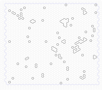
(a) $n=0.8$ and $x=0.55$.

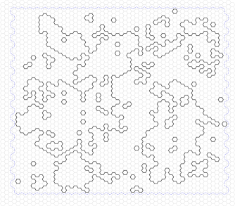
(b) $n=0.8$ and $x=0.6$.

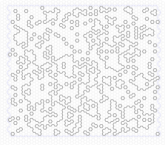
(c) $n=2$ and $x=1/\sqrt{2}\approx 0.707$.

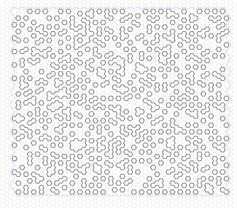
(d) $n=8$ and $x=1$.

Figure 7. A few samples of random loop configurations. Configurations are on a $60\times 45$ domain of type $0$ and are sampled via Glauber dynamics for 100 million iterations started from the empty configuration. The conjectured phase transition point for $n=0.8$ is $x_{c}=1/\sqrt{2+\sqrt{2-0.8}}\approx 0.568$ and for $n=2$ is $x_{c}=1/\sqrt{2}\approx 0.707$. Theorem 1.4 shows that long loops are exponentially unlikely for large $n$.

Spin O(n)

As described in the introduction, the loop $O(n)$ model can be viewed as an approximation of the spin $O(n)$ model, with the length of loops related to the spin-spin correlation function. Thus, our results prove an analogue of the well-known conjecture that spin-spin correlations decay exponentially (in the distance between the sites) in the planar spin $O(n)$ model with $n\geq 3$, at any positive temperature. Proving the conjecture itself remains a tantalizing challenge.

Small $n$

Studying the loop $O(n)$ model for small values of $n$ is of great interest. It is predicted that the model displays critical behavior only when $n\leq 2$. There, it is expected to undergo a Kosterlitz–Thouless phase transition at $x_{c}=1/\sqrt{2+\sqrt{2-n}}$, see [29], and exhibit conformal invariance when $x\geq x_{c}$. Mathematical results on this are currently restricted to the cases $n=1$ and $n=0$, which correspond to the Ising model and the self-avoiding walk, respectively. For these two cases, the critical values have been identified rigorously in [21] and [14], respectively. In the $n=1$ case, the model has been proved [6, 7] to be conformally invariant at $x_{c}=1/\sqrt{3}$. For $n=1$ and $x=\infty$ the height function of the model may be viewed as a uniformly chosen lozenge tiling of a domain in the plane. This viewpoint leads to a determinantal process, the dimer model, which has been analyzed in great detail (see, e.g., [19] for an introduction). Conformal invariance has also been proved for the double dimer model which is closely related to the case $n=2$ and $x=\infty$ (see [20]).

Our results are limited to the case $n\geq n_{0}$ and understanding the various behaviors for small values of $n$ remains a beautiful mathematical challenge. To give a taste of the different possibilities, we provide some simulation results in Figure 7.

Extremality and uniqueness of the Gibbs measures

When $n\geq n_{0}$ and $nx^{6}\geq C$, we prove that the model has at least three different Gibbs measures, distinguished by a choice of a sublattice of the triangular lattice. Are these the only extremal Gibbs measures in this regime (i.e., is every other measure a convex combination of these three measures)? Such a result would be in the spirit of the Aizenman–Higuchi theorem [1, 18] which proves that the only extremal Gibbs measures for the 2D Ising model are the two pure states. This theorem was recently extended to the $q$-state Potts model in [8].

For small values of $\max\{n,1\}x^{6}$, we prove the existence of a limiting Gibbs measure when exhausting space via an increasing sequence of domains with vacant boundary conditions. Is this Gibbs measure unique for each choice of $n$ and $x$ in this regime? Intuitively, the difficulty in proving this lies in dealing with domains with boundary conditions which force an interface (i.e., part of a loop) through the domain (similarly to the situation in Figure 3(b)). If this interface passes near the origin with non-negligible probability, one would obtain a limiting Gibbs measure having an infinite path with positive probability. However, one expects interfaces to follow diffusive scaling, similarly to random walk paths, and as such should have negligible probability to pass close to the origin when the domain is large. Making such an intuition rigorous is quite non-trivial and was recently carried out successfully in [8] for planar Potts models. Adapting the ideas in [8] to the loop $O(n)$ model poses a challenge as these rely on specific properties of the Potts model. Roughly, the strategy in [8] proceeds by showing that when starting from a large domain $H$ with arbitrary boundary conditions, only a uniformly bounded number of interfaces will reach the boundary of a smaller sub-domain $H^{\prime}$. Then it is shown that these bounded number of interfaces follow diffusive scaling as in the intuition above. The first part, bounding the number of interfaces between the boundary of $H$ and $H^{\prime}$, may possibly be carried out for the loop $O(n)$ model by using Lemma 1.9; configurations with many long interfaces may be ‘rewired’, erasing most of these interfaces and replacing them with short connections along the boundary of $H$, yielding configurations with much higher probability. The second part, however, showing the diffusive scaling, remains a major obstacle.

The hard-hexagon model

Our results shed light on the Gibbs measures of the loop $O(n)$ model when $n\geq n_{0}$ and either $nx^{6}\leq c$ or $nx^{6}\geq C$. The structure for $n\geq n_{0}$ and $c\leq nx^{6}\leq C$ remains unclear; see Figure 7(d) and Figure 2. Is there a single $x_{c}(n)$ at which the model transitions from the dilute, disordered phase to the dense, ordered phase? What happens when $x=x_{c}(n)$?

An intuition for this question may be obtained by considering a limiting model as $n$ tends to infinity. As noted already in the paper [9] where the loop $O(n)$ model was introduced, taking the limit $n\to\infty$ and $nx^{6}\to\lambda$ leads formally to the hard-hexagon model. As loops of length longer than $6$ become less and less likely in this limit, hard-hexagon configurations consist solely of trivial loops, with each such loop contributing a factor of $\lambda$ to the weight. Thus, the hard-hexagon model is the hard-core lattice gas model on the triangular lattice $\mathbb{T}$ with fugacity $\lambda$. For this model, Baxter [2] (see also [3, Chapter 14]) computed the critical fugacity

$$\lambda_{c}=\left(2\cos\left(\frac{\pi}{5}\right)\right)^{5}=\frac{1}{2}\left(11+5\sqrt{5}\right)\approx 11.09017,$$

and showed that as $\lambda$ increases beyond the threshold $\lambda_{c}$, the model undergoes a fluid-solid phase transition from a homogeneous phase in which the sublattice occupation frequencies are equal to a phase in which one of the three sublattices is favored. Additional information is obtained on the critical behavior including the fact that the mean density of hexagons is equal for each of the three sublattices [2, Equation (13)] and the fact that the transition is of second order [2, Equation (9)]. Baxter’s arguments use certain assumptions on the model which appear not to have been mathematically justified. Still, this exact solution may suggest that the loop $O(n)$ model with large $n$ will also have a unique transition point $x_{c}(n)$, that $nx_{c}(n)^{6}$ will converge to $\lambda_{c}$ as $n$ tends to infinity and that the transition in $x$ is of second order, with the model having a unique Gibbs state when $x=x_{c}(n)$.

Square-lattice random-cluster model and dilute Potts model

We start with a somewhat informal description of the square-lattice random-cluster model and refer the interested reader to [16, 12] for more details. The random-cluster model with parameters $0<p<1,q>0$ on a domain in $\mathbb{Z}^{2}$ is a random collection of edges $\eta$ of the domain whose probability is proportional to

$$p^{o(\eta)}(1-p)^{c(\eta)}q^{k(\eta)},$$

where $o(\eta)$ is the number of edges in $\eta$, $c(\eta)$ is the number of edges of the domain which are not in $\eta$ and $k(\eta)$ is the number of connected components in the graph whose vertices are the vertices of the domain and whose edges are given by $\eta$. For each $\eta$, one may draw a loop configuration $\omega_{\eta}$ (on the so-called medial lattice) consisting of the loops marking the boundaries of the connected components (these loops go around the connected components and on the boundary of each “hole” that the components surround); see Figure 8. It turns out that the probability of $\eta$ may be rewritten using these loops so that the probability of $\eta$ is proportional to

$$\lambda^{o(\eta)}(\sqrt{q})^{L(\omega_{\eta})},$$ (21)

where $\lambda:=\frac{p}{\sqrt{q}(1-p)}$ and $L(\omega_{\eta})$ is the number of loops in $\omega_{\eta}$. This representation highlights a self duality occurring when $p$ is such that $\lambda=1$ and this self-dual point has been proven to be the critical point $p_{c}(q)$ for the random-cluster model [4]. The formula (21) may immediately remind the reader of the formula for the probability of configurations in the loop $O(n)$ model given in Definition 1.1. However, we emphasize that $o(\eta)$ counts the number of edges in $\eta$ and as such is quite different from the ‘length’ of the loops in $\omega_{\eta}$. In fact, the loop configuration $\omega_{\eta}$ is necessarily fully packed in the domain for any given $\eta$, so that $\lambda$ plays a different role from the parameter $x$ of the loop $O(n)$ model. Still, the formula (21) does suggest an analogy between the random-cluster model at criticality (when $p=p_{c}(q)$) and the fully packed (i.e., $x=\infty$) loop $O(n)$ model with $n=\sqrt{q}$.

Figure 8. An illustration of a random-cluster configuration $\eta$ and its corresponding loop configuration $\omega_{\eta}$. The edges of $\eta$ are denoted by bold lines, the edges not in $\eta$ by dashed lines and the loops of $\omega_{\eta}$ by plain lines.

Taken with periodic boundary conditions on a square domain, the random-cluster model has two configurations $\eta$ which maximize $L(\omega_{\eta})$: one in which all the edges of the domain are absent (yielding loops around the vertices) and one in which all of them are present (yielding loops around the faces). These configurations are equally probable at the critical point, but one is preferred over the other whenever $p\neq p_{c}(q)$. Following a proof of Kotecký and Shlosman [23] for the closely-related Potts model, it has been proven by Laanait et al. [25] that for large $q$, the random-cluster model exhibits a first-order phase transition, so that at criticality there are two Gibbs states corresponding to the two ground states described above. Our results on the existence of the ordered phase for large $n$ and $x=\infty$ are quite analogous to this phenomenon. In fact, it is predicted that the square-lattice random-cluster model has a first-order phase transition if $q\geq 4$ and otherwise has a second-order phase transition. This is in line with the conjectured phase diagram for the loop $O(n)$ model, predicting that the ordered phase at $x=\infty$ exists only for $n\geq 2$.

We again point out that the parameter $p$ of the random-cluster model has no analogue in the loop $O(n)$ model and so the existence of a first-order transition in $p$ does not suggest that such a transition should occur also when varying $x$. As mentioned above, it may well be that for large $n$, the transition in $x$ is of second order by analogy with the situation for hard hexagons.

Lastly, we mention that Nienhuis [30] proposed a version of the Potts model, termed the dilute Potts model, with a direct relationship to the loop $O(n)$ model. A configuration of the dilute Potts model in a domain of the triangular lattice is an assignment of a pair $(s_{z},t_{z})$ to each vertex $z$ of the domain, where $s_{z}\in\{1,\ldots,q\}$ represents a spin and $t_{z}\in\{0,1\}$ denotes an occupancy variable. The probability of configurations involves a hard-core constraint that nearest-neighbor occupied sites must have equal spins (reminiscent of the Edwards-Sokal coupling of the Potts and random-cluster models) and single-site, nearest-neighbor and triangle interaction terms involving the occupancy variables. With a certain choice of coupling constants, the marginal of the model on the occupancy variables is equivalent to the loop $O(n)$ model (with $n=\sqrt{q}$), with the loops being the interfaces between occupied and unoccupied sites. Nienhuis predicts this choice of parameters to be part of the critical surface of the dilute Potts model. The properties of the dilute Potts model appear not to have been studied in the mathematical literature and it would be interesting to see whether they can shed further light on the behavior of the loop $O(n)$ model.

Height representation for integer $n$

When the loop parameter $n$ is an integer, the loop $O(n)$ model admits a height function representation [9]. Let $T_{n}$ be the $n$-regular tree (so that $T_{1}=\{+,-\}$ and $T_{2}=\mathbb{Z}$) rooted at an arbitrary vertex $\rho$. Let $\text{Lip}_{n}$ be the set of functions $\varphi\colon\mathbb{T}\to T_{n}$ satisfying the ‘Lipschitz condition’:

If $$y,z\in\mathbb{T} \varphi(y)=\varphi(z) \varphi(y) \varphi(z) T_{n}$$ are adjacent then either or is adjacent to in

(in other words, $\varphi$ is a graph homomorphism from $\mathbb{T}$ to the graph $T_{n}^{\prime}$ obtained from $T_{n}$ by adding a loop at every vertex). For a domain $H\subset\mathbb{H}$, we further set $\text{Lip}_{n}(H)$ to be the set of $\varphi\in\text{Lip}_{n}$ satisfying the boundary condition $\varphi(z)=\rho$ for all hexagons $z$ which are not in the interior of $H$ (i.e., which are incident to a vertex in $V(\mathbb{H})\setminus V(H)$). Define the ‘level lines’ of $\varphi\in\text{Lip}_{n}$ by

$$\omega_{\varphi}:=\big{\{}e\in E(\mathbb{H})\,:\,\text{the edge $e$ borders hexagons $y,z\in\mathbb{T}$ satisfying $\varphi(y)\neq\varphi(z)$}\big{\}}.$$

Observe that $\omega_{\varphi}$ is a loop configuration and that if $\varphi\in\text{Lip}_{n}(H)$ then $\omega_{\varphi}\in\mathsf{LoopConf}(H,\emptyset)$. For a real parameter $x>0$, define a probability measure $\nu_{H,n,x}$ on $\text{Lip}_{n}(H)$ by

$$\nu_{H,n,x}(\varphi):=\frac{x^{|\omega_{\varphi}|}}{Z^{\text{Lip}}_{H,n,x}},\quad\varphi\in\text{Lip}_{n}(H),$$

where $Z^{\text{Lip}}_{H,n,x}$ is the unique constant which makes $\nu_{H,n,x}$ a probability measure. The definition is extended to $x=\infty$ by $\nu_{H,n,\infty}(\varphi):=\lim_{x\to\infty}\nu_{H,n,x}(\varphi)$.

The fact that the loop $O(n)$ model admits a height function representation is manifested in the relation between the measures $\nu_{H,n,x}$ and $\mathbb{P}_{H,n,x}^{\emptyset}$. As is straightforward to verify, if $\varphi$ is a random function chosen according to $\nu_{H,n,x}$ then $\omega_{\varphi}$ is distributed according to $\mathbb{P}_{H,n,x}^{\emptyset}$. In particular, the height function representation of the loop $O(1)$ model is an Ising model (which may be either ferromagnetic or antiferromagnetic according to whether $x<1$ or $x>1$) and the height function representation of the loop $O(2)$ model is a restricted Solid-On-Solid model. Our main result, Theorem 1.4, implies that long level lines surrounding a given hexagon are exponentially unlikely in height functions sampled according to $\nu_{H,n,x}$, when $H$ is a domain of type ${{\mathsf{c}}}\in\{0,1,2\}$ and $n$ is large. Our proof does not make use of the height function representation and thus applies to real $n$. It would be interesting to see whether the height function representation may be used to provide further information for integer $n$.

Appendix A Integrals

In this section, we present a detailed derivation of the formulas approximating the partition function and the spin-spin correlations in the spin $O(n)$ model on a finite subgraph $H$ of the hexagonal lattice. Let $u,v\in V(H)$ be distinct vertices and let $H^{+}$ be the (possibly multi-)graph obtained by adding an edge $e_{u,v}$ between $u$ and $v$ to $H$. In the introductory section, the derivation was reduced to computing integrals of the form

$$I(\omega):=\int_{\Omega}\prod_{\{w,w^{\prime}\}\in E(\omega)}\langle\sigma_{w},\sigma_{w^{\prime}}\rangle\,d\sigma,$$

where $\Omega=(\sqrt{n}\cdot\mathbb{S}^{n-1})^{V(H)}$, $\omega$ is an arbitrary subgraph of $H^{+}$, and $d\sigma$ is the product of $|V(H)|$ uniform probability measures on $\sqrt{n}\cdot\mathbb{S}^{n-1}$. Note first that, by symmetry, making the substitution $\sigma_{w}\leftarrow-\sigma_{w}$ for some $w\in V(H)$ does not change the value of this integral and consequently $I(\omega)=0$ unless every vertex has even degree in $\omega$. In other words, if $\omega\subset H$ then $I(\omega)=0$ unless $\omega$ is a loop configuration, i.e., $\omega\in\mathsf{LoopConf}(H,\emptyset)$, and $I(\omega+e_{u,v})=0$ unless the degrees of $u$ and $v$ in $\omega$ are odd and the degrees of all other vertices are even, i.e., $\omega\in\mathsf{LoopConf}(H,\emptyset,u,v)$.

We shall repeatedly make use of the following identity. For every $x,y\in\mathbb{R}^{n}$,

$$\int_{\sqrt{n}\cdot\mathbb{S}^{n-1}}\langle x,z\rangle\langle z,y\rangle\,dz=\langle x,y\rangle,$$ (22)

where $dz$ is the uniform probability measure on $\sqrt{n}\cdot\mathbb{S}^{n-1}$. Note that both sides of (22) are bilinear functions of $x$ and $y$ and therefore it is enough to verify that (22) holds when $x$ and $y$ are two vectors from the canonical basis $\{e_{1},\ldots,e_{n}\}$ of $\mathbb{R}^{n}$. By symmetry, for each $i$,

$$\int_{\sqrt{n}\cdot\mathbb{S}^{n-1}}\langle e_{i},z\rangle\langle z,e_{i}\rangle\,dz=\frac{1}{n}\sum_{i=1}^{n}\int_{\sqrt{n}\cdot\mathbb{S}^{n-1}}\langle z,e_{i}\rangle^{2}\,dz=\frac{1}{n}\int_{\sqrt{n}\cdot\mathbb{S}^{n-1}}\|z\|^{2}dz=1,$$

If $i\neq j$, substituting $(z_{1},\ldots,z_{n})\leftarrow(z_{1},\ldots,z_{i-1},-z_{i},z_{i+1},\ldots,z_{n})$ yields

$$\int_{\sqrt{n}\cdot\mathbb{S}^{n-1}}\langle e_{i},z\rangle\langle z,e_{j}\rangle\,dz=-\int_{\sqrt{n}\cdot\mathbb{S}^{n-1}}\langle e_{i},z\rangle\langle z,e_{j}\rangle\,dz=0.$$

Suppose first that $\omega\in\mathsf{LoopConf}(H,\emptyset)$. Since the loops of $\omega$ are vertex-disjoint, $I(\omega)=\prod_{L\subset\omega}I(L)$, where $L$ ranges over all loops of $\omega$. Suppose now that $L$ is a loop through vertices $v_{0},\ldots,v_{\ell}$, where $v_{\ell}=v_{0}$. Invoking (22) repeatedly yields

$$\begin{split}I(L)&=\int_{\Omega}\langle\sigma_{v_{0}},\sigma_{v_{1}}\rangle\cdots\langle\sigma_{v_{\ell}-1},\sigma_{v_{\ell}}\rangle\,d\sigma=\int_{\Omega}\langle\sigma_{v_{0}},\sigma_{v_{0}}\rangle\,d\sigma=n,\end{split}$$

giving $I(\omega)=n^{L_{H}(\omega)}$.

Suppose now that $\omega\in\mathsf{LoopConf}(H,\emptyset,u,v)$, let $C$ be the connected component of $u$ (and $v$) in $\omega$, and note that $C$ must contain a simple path $P$ connecting $u$ and $v$. Since we have already proved that $I(L)=n$ for every loop $L$, in order to compute $I(\omega+e_{u,v})$, it is enough to compute $I(C+e_{u,v})$. A simple case analysis shows that $C$ is either (i) the path $P$, (ii) the path $P$ and a loop intersecting $P$ in one of its endpoints, (iii) the path $P$ and two vertex-disjoint loops, each intersecting $P$ in one of its endpoints, or (iv) the path $P$ and two other simple paths connecting $u$ and $v$, each pair of paths sharing only the vertices $u$ and $v$. Since the edge $e_{u,v}$ closes $P$ into a loop, invoking (22) repeatedly to ‘contract’ loops yields that $I(C+e_{u,v})$ equals $n$ in case (i), $n^{2}$ in case (ii), and $n^{3}$ in case (iii). In case (iv), invoking (22) repeatedly only gives

$$I(C+e_{u,v})=\iint_{\sqrt{n}\cdot\mathbb{S}^{n-1}}\langle x,y\rangle^{4}\,dxdy,$$

which is somewhat more difficult to compute. Using symmetry and the fact that the projection of the Lebesgue measure on $\mathbb{S}^{n-1}\subset\mathbb{R}^{n}$ onto the first coordinate gives the measure on $[-1,1]$ with density $(1-t^{2})^{\frac{n-3}{2}}$ up to a normalization constant, we obtain

$$\begin{split}I(C+e_{u,v})&=\int_{\sqrt{n}\cdot\mathbb{S}^{n-1}}\langle x,\sqrt{n}e_{1}\rangle^{4}\,dx=n^{4}\int_{\sqrt{n}\cdot\mathbb{S}^{n-1}}\langle x/\sqrt{n},e_{1}\rangle^{4}\,dx\\ &=n^{4}\cdot\frac{\int_{-1}^{1}t^{4}(1-t^{2})^{\frac{n-3}{2}}\,dt}{\int_{-1}^{1}(1-t^{2})^{\frac{n-3}{2}}\,dt}=\frac{3n^{3}}{n+2},\end{split}$$

where one may obtain the final identity using integration by parts.

Appendix B Circuits and domains

Here we prove some facts about circuits and domains.

Proof of Fact 2.1.

Let $\gamma$ be a circuit and denote by $\mathbb{H}_{\gamma}$ the subgraph of $\mathbb{H}$ obtained by removing from $\mathbb{H}$ all edges in $\gamma^{*}$. Let $\mathrm{Ext}(\gamma)$ be the set of vertices that are the endpoint of some infinite simple path in $\mathbb{H}_{\gamma}$.

First, we claim that $\mathrm{Ext}(\gamma)$ is a connected component of $\mathbb{H}_{\gamma}$. To see this, note first that by definition, $\mathrm{Ext}(\gamma)$ is a union of connected components of $\mathbb{H}_{\gamma}$. Furthermore, since $\gamma^{*}$ is finite, there exists an $R$ and a vertex $u\in V(\mathbb{H})$ such that the complement of the ball of radius $R$ (in the graph distance determined by $\mathbb{H}$) centered at $u$ induces the same connected graph $\mathbb{H}_{R}$ in both $\mathbb{H}$ and $\mathbb{H}_{\gamma}$. Finally, every infinite simple path in $\mathbb{H}$ intersects $\mathbb{H}_{R}$ and therefore $\mathrm{Ext}(\gamma)$ consists of a single connected component.

Second, we claim that the set of endpoints of the edges in $\gamma^{*}$ intersects at most two connected components of $\mathbb{H}_{\gamma}$, one of which is $\mathrm{Ext}(\gamma)$. To see this, suppose that $\gamma=(\gamma_{0},\ldots,\gamma_{m})$ as in the definition in Section 2.1. In order to prove the first part of our claim, it suffices to show that for each $i\in\{1,\ldots,m-1\}$, there are two disjoint $\mathbb{H}_{\gamma}$-connected sets of vertices, each of which intersects both $\{\gamma_{i-1},\gamma_{i}\}^{*}$ and $\{\gamma_{i},\gamma_{i+1}\}^{*}$ (where we regard an edge as the set of its endpoints). To see this, note that $\{\gamma_{i-1},\gamma_{i}\}^{*}$ and $\{\gamma_{i},\gamma_{i+1}\}^{*}$ are the only two out of six edges surrounding the hexagon $\gamma_{i}$ that belong to $\gamma^{*}$. Consequently, the removal of $\gamma^{*}$ partitions the six vertices surrounding $\gamma_{i}$ into two $\mathbb{H}_{\gamma}$-connected sets, each of which intersects both $\{\gamma_{i-1},\gamma_{i}\}^{*}$ and $\{\gamma_{i},\gamma_{i+1}\}^{*}$. For the second part of the claim, consider an arbitrary infinite simple path in $\mathbb{H}$ which uses an edge from $\gamma^{*}$. Let $\{v,w\}$ be the last edge of $\gamma^{*}$ on this path and observe that either $v$ or $w$ belongs to $\mathrm{Ext}(\gamma)$. Hence, $\mathrm{Ext}(\gamma)$ is one of the $\mathbb{H}_{\gamma}$-connected components that contains an endpoint of an edge of $\gamma^{*}$.

Third, we claim that $\mathrm{Ext}(\gamma)\neq V(\mathbb{H})$. If this were not the case, then in particular there would be a $\{v,w\}\in\gamma^{*}$ such that both $v$ and $w$ belong to the same connected component of $\mathbb{H}_{\gamma}$. Consequently, there would be a simple path $P$ in $\mathbb{H}_{\gamma}$ that connects $v$ and $w$. The edge $\{v,w\}$ and $P$ would then form a cycle in $\mathbb{H}$ that contains exactly one edge of $\gamma^{*}$. This is impossible since the basic $6$-cycles surrounding the hexagons of $\mathbb{T}$ generate the cycle space of $\mathbb{H}$ and each of these basic cycles intersects $\gamma^{*}$ in either $0$ or $2$ edges.

Fourth, we claim that $V(\mathbb{H})\setminus\mathrm{Ext}(\gamma)$ is $\mathbb{H}_{\gamma}$-connected, that is, every two $v,w\notin\mathrm{Ext}(\gamma)$ are in the same connected component of $\mathbb{H}_{\gamma}$. To see this, consider two infinite simple paths $P_{v}$ and $P_{w}$ in $\mathbb{H}$ that start at $v$ and $w$, respectively. Since $v,w\notin\mathrm{Ext}(\gamma)$, both $P_{v}$ and $P_{w}$ contain an edge from $\gamma^{*}$. Let $v^{\prime},w^{\prime}$ be the first vertices in $P_{v}$ and $P_{w}$, respectively, which are incident to edges of $\gamma^{*}$. Clearly $v,v^{\prime}$ and $w,w^{\prime}$ lie in the same $\mathbb{H}_{\gamma}$-connected components, other than $\mathrm{Ext}(\gamma)$. By our second claim, $v^{\prime}$ and $w^{\prime}$ must belong to the same $\mathbb{H}_{\gamma}$-connected component. Hence, $v$ and $w$ also belong to the same $\mathbb{H}_{\gamma}$-connected component, which we shall from now on denote by $\mathrm{Int}(\gamma)$.

Finally, we show that both $\mathrm{Ext}(\gamma)$ and $\mathrm{Int}(\gamma)$, as $\mathbb{H}_{\gamma}$-connected components, are induced subgraphs of $\mathbb{H}$ and that $\mathrm{Int}(\gamma)$ is finite. The first assertion follows from the fact that the two endpoints of each edge of $\gamma^{*}$ belong to different $\mathbb{H}_{\gamma}$-connected components, which we have already established above. If the second assertion were false, then $\mathrm{Int}(\gamma)$ would be an infinite $\mathbb{H}_{\gamma}$-connected graph and hence it would contain an infinite simple path, contradicting the fact that $\mathrm{Int}(\gamma)\cap\mathrm{Ext}(\gamma)=\emptyset$. ∎

Proof of Fact 2.2.

Let $H$ be a domain and let $E$ be the set of edges of $\mathbb{H}$ with exactly one endpoint in $V(H)$. Let $T$ be the auxiliary graph with vertex set $\mathbb{T}$ whose edges are all pairs $\{y,z\}$ such that $\{y,z\}^{*}\in E$. We first claim that all vertex degrees in $T$ are even. Indeed, to see this for the degree of a hexagon $z\in\mathbb{T}$, it suffices to traverse the vertices bordering $z$ in order and to consider which of them belong to $V(H)$. It follows that $T$ contains a circuit $\gamma$. By Fact 2.1, $\gamma^{*}$ splits $\mathbb{H}$ into exactly two connected components. As $\gamma^{*}\subseteq E$ and $\mathrm{Int}(\gamma)$ is finite and non-empty, and as $V(H)$ is finite, connected and with connected complement, it must be that $V(\mathbb{H})\setminus V(H)\subseteq\mathrm{Ext}^{\mathrm{V}}(\gamma)$ and $V(H)\subseteq\mathrm{Int}^{\mathrm{V}}(\gamma)$. Consequently, $H=\mathrm{Int}(\gamma)$. ∎

Proof of Fact 2.3.

Denote $A:=\mathrm{Int}^{\mathrm{V}}(\sigma)$, $A^{\prime}:=\mathrm{Int}^{\mathrm{V}}(\sigma^{\prime})$ and $B:=A\cup A^{\prime}$. Let us first show that $B$ is connected. If $A\cap A^{\prime}\neq\emptyset$ then this is immediate. Otherwise, by assumption, there exists an edge $\{v,u\}\in\sigma^{*}\cap(\sigma^{\prime})^{*}$. Assume without loss of generality that $v\in A$ and $u\notin A$. Then $u\in A^{\prime}$ and $v\notin A^{\prime}$, and thus, $B$ is connected.

Let $C$ be the unique infinite connected component of $V(\mathbb{H})\setminus B$ and let $D:=V(\mathbb{H})\setminus C$. It is straightforward to check that $D$ is finite, $B\subset D$ and $\partial D\subset\partial B$. Since $B$ is connected, this implies that $D$ is connected. Thus, as $V(\mathbb{H})\setminus D=C$ is connected, the subgraph of $\mathbb{H}$ induced by $D$ is a domain.

By Fact 2.2, there exists a circuit $\gamma$ such that $D=\mathrm{Int}^{\mathrm{V}}(\gamma)$. It remains to check that $\gamma^{*}\subset\sigma^{*}\cup(\sigma^{\prime})^{*}$. Let $\{v,u\}\in\gamma^{*}$ be such that $v\in D$ and $u\notin D$. In particular, $v\in B$ and $u\notin B$. Thus, either $v\in A$ so that $\{v,u\}\in\sigma^{*}$, or $v\in A^{\prime}$ so that $\{v,u\}\in(\sigma^{\prime})^{*}$. ∎

References

- [1] Michael Aizenman, Translation invariance and instability of phase coexistence in the two-dimensional Ising system, Comm. Math. Phys. 73 (1980), no. 1, 83–94. MR 573615 (82c:82003)
- [2] Rodney J. Baxter, Hard hexagons: exact solution, J. Phys. A 13 (1980), no. 3, L61–L70. MR 560533 (80m:82052)
- [3] by same author, Exactly solved models in statistical mechanics, Academic Press Inc. [Harcourt Brace Jovanovich Publishers], London, 1989, Reprint of the 1982 original. MR 998375 (90b:82001)
- [4] Vincent Beffara and Hugo Duminil-Copin, The self-dual point of the two-dimensional random-cluster model is critical for , Probab. Theory Related Fields 153 (2012), no. 3-4, 511–542. MR 2948685
- [5] Béla Bollobás, The art of mathematics, Cambridge University Press, New York, 2006, Coffee time in Memphis. MR 2285090 (2007h:00005)
- [6] Dmitry Chelkak, Hugo Duminil-Copin, Clément Hongler, Antti Kemppainen, and Stanislav Smirnov, Convergence of Ising interfaces to Schramm’s SLE curves, C. R. Math. Acad. Sci. Paris 352 (2014), no. 2, 157–161. MR 3151886
- [7] Dmitry Chelkak and Stanislav Smirnov, Universality in the 2D Ising model and conformal invariance of fermionic observables, Invent. Math. 189 (2012), no. 3, 515–580. MR 2957303
- [8] L. Coquille, H. Duminil-Copin, D. Ioffe, and Y. Velenik, On the Gibbs states of the noncritical Potts model on , Probability Theory and Related Fields 158 (2014), 477–512.
- [9] Eytan Domany, D Mukamel, Bernard Nienhuis, and A Schwimmer, Duality relations and equivalences for models with O(n) and cubic symmetry, Nuclear Physics B 190 (1981), no. 2, 279–287.
- [10] C. Domb and M.S. Green, Phase transitions and critical phenomena, vol. 3, Academic New-York Press, 1976.
- [11] Hugo Duminil-Copin, Parafermionic observables and their applications to planar statistical physics models, Ensaios Matematicos, vol. 25, Brazilian Mathematical Society, 2013.
- [12] Hugo Duminil-Copin, Geometric representations of lattice spin models, Spartacus Graduate, Cours Peccot, Collège de France (2015).
- [13] Hugo Duminil-Copin and Stanislav Smirnov, Conformal invariance of lattice models, Probability and statistical physics in two and more dimensions, Clay Math. Proc., vol. 15, Amer. Math. Soc., Providence, RI, 2012, pp. 213–276. MR 3025392
- [14] by same author, The connective constant of the honeycomb lattice equals , Ann. of Math. (2) 175 (2012), no. 3, 1653–1665. MR 2912714
- [15] Jürg Fröhlich and Thomas Spencer, The Kosterlitz-Thouless transition in two-dimensional Abelian spin systems and the Coulomb gas, Comm. Math. Phys. 81 (1981), no. 4, 527–602. MR 634447 (83b:82029)
- [16] Geoffrey R Grimmett, The random-cluster model, vol. 333, Springer Science & Business Media, 2006.
- [17] G. Heller and H.A. Kramers, Ein Klassisches Modell des Ferromagnetikums und seine nachträgliche Quantisierung im Gebiete tiefer Temperaturen, Ver. K. Ned. Akad. Wetensc.(Amsterdam) 37 (1934), 378–385.
- [18] Y. Higuchi, On the absence of non-translation invariant Gibbs states for the two-dimensional Ising model, Random fields, Vol. I, II (Esztergom, 1979), Colloq. Math. Soc. János Bolyai, vol. 27, North-Holland, Amsterdam, 1981, pp. 517–534. MR 712693 (84m:82020)
- [19] Richard Kenyon, An introduction to the dimer model, School and Conference on Probability Theory, ICTP Lect. Notes, XVII, Abdus Salam Int. Cent. Theoret. Phys., Trieste, 2004, pp. 267–304 (electronic).
- [20] by same author, Conformal invariance of loops in the double-dimer model, Comm. Math. Phys. 326 (2014), no. 2, 477–497.
- [21] D Kim and RI Joseph, Exact transition temperature of the potts model with q states per site for the triangular and honeycomb lattices, Journal of Physics C: Solid State Physics 7 (1974), no. 8, L167.
- [22] JM Kosterlitz and DJ Thouless, Ordering, metastability and phase transitions in two-dimensional systems, Journal of Physics C: Solid State Physics 6 (1973), no. 7, 1181–1203.
- [23] R. Kotecký and S. B. Shlosman, First-order phase transitions in large entropy lattice models, Comm. Math. Phys. 83 (1982), no. 4, 493–515. MR 649814 (83i:82033)
- [24] Antti J. Kupiainen, On the expansion, Comm. Math. Phys. 73 (1980), no. 3, 273–294. MR 574175 (81g:82007)
- [25] Lahoussine Laanait, Alain Messager, Salvador Miracle-Solé, Jean Ruiz, and Senya Shlosman, Interfaces in the Potts model. I. Pirogov-Sinai theory of the Fortuin-Kasteleyn representation, Comm. Math. Phys. 140 (1991), no. 1, 81–91. MR 1124260 (93d:82021a)
- [26] W. Lenz, Beitrag zum Verständnis der magnetischen Eigenschaften in festen Körpern., Phys. Zeitschr. 21 (1920), 613–615.
- [27] Oliver A. McBryan and Thomas Spencer, On the decay of correlations in -symmetric ferromagnets, Comm. Math. Phys. 53 (1977), no. 3, 299–302. MR 0441179 (55 #14043)
- [28] N David Mermin and H Wagner, Absence of ferromagnetism or antiferromagnetism in one-or two-dimensional isotropic Heisenberg models, Physical Review Letters 17 (1966), 1133–1136.
- [29] Bernard Nienhuis, Exact Critical Point and Critical Exponents of Models in Two Dimensions, Physical Review Letters 49 (1982), no. 15, 1062–1065.
- [30] Bernard Nienhuis, Locus of the tricritical transition in a two-dimensional q-state potts model, Physica A: Statistical Mechanics and its Applications 177 (1991), no. 1-3, 109–113.
- [31] J. Palmer, Planar Ising correlations, Progress in Math. Physics, vol. 49, Birkhäuser Boston Inc., Boston, MA, 2007.
- [32] R. Peierls, On Ising’s model of ferromagnetism., Math. Proc. Camb. Phil. Soc. 32 (1936), 477–481.
- [33] A Polyakov, Interaction of goldstone particles in two dimensions. Applications to ferromagnets and massive Yang-Mills fields, Physics Letters B 59 (1975), no. 1, 79–81.
- [34] H.E. Stanley, Dependence of critical properties on dimensionality of spins, Physical Review Letters 20 (1968), no. 12, 589–592.
- [35] DJ Thouless, Long-range order in one-dimensional Ising systems, Physical Review 187 (1969), 732–733.
- [36] V.G. Vaks and A.I. Larkin, On Phase Transitions of Second Order, Soviet Journal of Experimental and Theoretical Physics 22 (1966), 678.