An method for the radiative transport equation in three dimensions
Manabu Machida
Department of Mathematics, University of Michigan,
Ann Arbor, MI 48109, USA
mmachida@umich.edu
Abstract
The method is an accurate and efficient numerical method for the
one-dimensional radiative transport equation. In this paper the method
is extended to three dimensions using rotated reference frames. To
demonstrate the method, the exiting flux from structured illumination
reflected by a medium occupying the half space is calculated.
pacs:
05.60.Cd, 42.68.Ay, 95.30.Jx
1 Introduction
We consider light propagating in a homogeneous random medium occupying
the half-space () with the boundary at . The specific
intensity (, ) of light obeys
the following radiative transport equation.
(1)
where is the incident beam and is the
internal source. Let and
be the cosine of the polar angle and the azimuthal angle
of . Here is the
albedo for single scattering. Using the absorption and scattering
parameters and , we have , where
is the total attenuation. The above form (1)
implies that is normalized by . Furthermore
is the scattering phase function which is normalized as
The radiative transport equation or the linear Boltzmann equation governs
transport processes of noninteracting particles such as neutrons in a reactor
as well as light propagation in random media such as fog, clouds, and
biological tissue.
In this paper we will present a numerical method of solving (1)
by extending the method ( stands for facile) to three dimensions.
The method first developed by Siewert [51] is a method of
obtaining the specific intensity in one dimension making use of orthogonality
relations of singular eigenfunctions [4, 6, 10]. The use of
rotated reference frames [43, 48, 50] makes
it possible to extend the method to three dimensions.
In 1960 Case considered the time-independent one-dimensional radiative
transport
equation with isotropic scattering and solved the equation with separation
of variables by finding singular eigenfunctions [4]. The method
was soon extended to the case of anisotropic scattering without
[44, 47] and with
[45] azimuthal dependence. Such singular-eigenfunction
approach is sometimes called Caseology. In this method, solutions to
the one-dimensional radiative transport equation are given by a superposition
of singular eigenfunctions. The existence and uniqueness of such solutions
were proved [25, 26, 27, 28]. In the method,
there is no need of evaluating singular functions although the fact that
the specific intensity consists of singular eigenfunctions is used.
In one dimension, the radiative transport equation
was solved by the method in the slab geometry for isotropic scattering
[12, 52] and anisotropic scattering
without [9, 16, 51] and with
[19, 20] azimuthal dependence.
The method was also extended to multigroup [14].
After finding the specific intensity on the boundary, we can further calculate
the specific intensity inside the medium [16].
The uniqueness of the solution to the key equation was proved
[29].
For isotropic scattering, the three dimensional radiative transport equation
was solved with the method [11, 53]
using the pseudo-problem [55], which is based on plane-wave
decomposition. See the review article by Garcia [13].
In 1964 Dede used rotated reference frames to solve the three-dimensional
radiative transport equation with the method [8]. Dede
pointed out that equations in three dimensions reduce to one-dimensional
equations if reference frames are rotated in the direction of the Fourier
vector. Kobayashi developed Dede’s calculation and computed coefficients
in the expansion by solving a three-term recurrence relation
recursively starting with the initial term [24]. In 2004
Markel obtained the coefficients in terms of eigenvalues and eigenvectors of
the tridiagonal matrix originating from the three-term recurrence relation,
and showed that the specific intensity can be efficiently computed
[43]. With the use of eigenvalues, the relation to Case’s method
became visible. This new formulation can be viewed as separation
of variables in which the eigenvalues are separation constants
[50]. Moreover it was found that any complex unit
vector can be used to rotate reference frames [48]. This
generalization makes it possible to solve boundary value problems in the form
of plane-wave decomposition [41]. It was then found that the
structure of separation of variables implies Case’s method in rotated
reference frames [42]. Thus the singular-eigenfunction approach
was extended to three dimensions. Indeed the method of rotated
reference frames is a three-dimensional extension of the
spherical-harmonic expansion
[1, 49] in Caseology.
The usefulness of the method of rotated reference frames has been numerically
justified for a two-dimensional rectangular domain [24],
a three-dimensional infinite medium [43, 48],
the slab geometry in three dimensions [41],
in flatland [30, 31, 38],
in the half-space geometry [33, 35, 36, 37, 39], and
the time-dependent equation in an infinite medium [32, 34].
The method was also used to experimentally determine optical properties of
turbid media [56, 57]. It is expected that
more accurate numerical values are obtained if higher terms in the series
are taken into account.
Although the method of rotated reference frames is an efficient method,
the obtained values become unstable when high-degree spherical
harmonics are used. The three-dimensional method
developed in the present paper does not suffer from this instability.
By assuming that scatterers are spherically symmetric, we model
as
(2)
where , and , for .
Moreover are Legendre polynomials and are spherical harmonics.
We introduce the scattering asymmetry parameter as
(). The Henyey-Greenstein model
[22] is obtained in the limit .
Let us define
We similarly define and .
Let us express the upper and lower hemispheres as
.
We expand the Fourier transform of the reflected light
() as
(3)
where is the highest degree of the expansion
(). Only same-parity degrees
are taken because the three-term recurrence relation of associated Legendre
polynomials implies that of opposite-parity are not independent
[20, 48]. This expansion in (3) can
be compared to the method [6], but the method is
more efficient because the spatial dependence of the specific intensity is
analytically given and the orthogonality relation among three-dimensional
singular eigenfunctions can be used (see §2.3).
On the other hand, is given as a linear combination
of eigenmodes [42],
for which notations are introduced in §2.3. They satisfy
orthogonality relations. For simplicity let us assume .
Making use of the fact that contains only decaying modes, we have
(See (34) for the general case)
(4)
The above equation results in a linear system for .
The specific intensity of the reflected light is then calculated as
where .
Remark 1.1.
Isotropic scattering is possible. However we need to change
the collocation scheme for obtaining . For the sake of simplicity,
we assume in this paper.
Remark 1.2.
The expansion in (3) can be compared to the method of
rotated reference frames, which expands every eigenmode with
spherical harmonics:
(5)
with some coefficients . This causes
numerical instability regardless of and
when is increased to achieve higher precision.
For example, let us consider a simple case of , ,
, and . Noting that
, we see
that the right-hand side of (5) is a polynomial of
. On the left-hand side, we have
. This series is
divergent if . In general, the instability takes
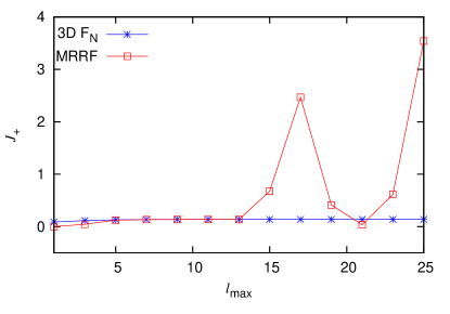
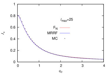
place due to the same mechanism. Figure 1 shows
the exiting current on the boundary () as a function of .
See §4 for the details.
Figure 1:
The exitance (44) is plotted as a function of
for , , and .
We set .
The remainder of the paper is organized as follows. In §2 we
introduce singular eigenfunctions and rotated reference frames. In §3
we consider the method in three dimensions. The key equation is
obtained in (35), from which the coefficients in
(3) are computed.
In §4 the three-dimensional method is
numerically tested for structured illumination. Section 5 is
devoted to concluding remarks. Finally structured illumination by
the method of rotated reference frames is summarized in
A.
2 Preliminaries
To develop the method in three dimensions in §3,
we give brief reviews and define our notations in this section.
In §2.1, we introduce polynomials and .
In §2.2, Case’s singular-eigenfunction approach is explained.
In §2.3, we give a review on singular eigenfunctions in
three dimensions.
In §2.4, it is sketched how the method of rotated reference frames
is obtained using three-dimensional singular eigenfunctions.
The normalized Chandrasekhar polynomials (, ,
) are given by the three-term recurrence relation
(6)
with the initial term
(7)
We note that
The polynomials are obtained if we multiply Chandrasekhar polynomials
[7] by [54].
Definition 2.3.
The polynomials (, ) are introduced as
(8)
where is the Legendre polynomial of degree and is
the associated Legendre polynomial of degree and order .
We have
The polynomials satisfy the three-term recurrence relation
(9)
with
and the orthogonality relation
2.2 Singular eigenfunctions for one dimension
We will first investigate the one-dimensional homogeneous radiative
transport equation (10) and then consider the three dimensional
equation (26). Let us begin with
(10)
where , and is given
in (2). Separated solutions to (10) are given by
[4, 45, 47]
(11)
where is a separation constant, ()
is an integer, and
where denotes the Cauchy principal value. Here the separation
constant has discrete values
(, ) and the continuous spectrum between
and . The number of discrete eigenvalues depends on
and . The function is given by
Discrete eigenvalues satisfy
where for
By using , we can readily check that
in (15) satisfy
. This implies . Singular
eigenfunctions satisfy
[4, 45, 47]
where the Kronecker delta is replaced by the Dirac delta
if are in the continuous spectrum. The
normalization factor is given by
(17)
where .
We can numerically obtain the discrete eigenvalues
as eigenvalues of a tridiagonal matrix below. For
() and (), the matrix is given by
(18)
where . The matrix has
or positive eigenvalues for even
or odd, respectively. To see how is obtained, we first prove
the following proposition.
We note that (), where
is the associated Legendre polynomial of the second kind. Therefore
we obtain
Thus the proof is completed.
∎
Let us recall that the recurrence relation
(6) for is derived for an eigenvalue in
(11) and rewrite (6) as
Hence eigenvalues of are zeros of . Together with
Proposition 2.4, we see that discrete eigenvalues can be
computed as eigenvalues of for sufficiently large . More
sophisticated ways of obtaining discrete eigenvalues are discussed in
Ref. [17].
The tridiagonal matrix can be alternatively obtained as follows.
Let us write as
Using the orthogonality relation for associated Legendre polynomials:
,
we obtain
The above equation forms an eigenvalue problem for , and
are given in terms of eigenvectors of .
2.3 Singular eigenfunctions for three dimensions
Definition 2.5(Rotated reference frames).
Let be a unit vector such that .
We define an invertible linear operator
. For a function (),
is the value of where is measured in
the rotated reference frame whose -axis lies in the direction of .
Since Wigner’s -matrices are given in terms of
, we also write
To compute Wigner’s -matrices, we take square roots such that
for all
[48, 41]. We have
and
In particular we obtain
where is the polar angle of .
Let us consider
(26)
where , . Solutions to the above
equation are given by a superposition of eigenmodes
(27)
where . To see this we substitute the separated
solution (27) in the above homogeneous three-dimensional
radiative transport equation (26) and obtain
(28)
The right-hand side can be written as
(29)
That is,
Thus the three-dimensional equation (28) reduces to the
one-dimensional equation (13). Recall that
given in (12) is constructed so that (13) obtained from
(10) and (11) is satisfied. We have
(30)
Proposition 2.12.
The following orthogonality relation holds.
Proof.
The full-range orthogonality is obtained in [42]
through the Green’s function. Here we give a direct proof.
We perform separation of variables to the homogeneous equation by assuming
the form (27). By substituting the separated solution into
the radiative transport equation (26), we obtain
For fixed , we consider and .
Let us write ,
. We write the following two equations.
We note (24). By subtraction and integration over we have
where the normalization factor is given in
(17). Thus we obtain the full-range orthogonality relation.
∎
2.4 Method of rotated reference frames
The method of rotated reference frames does not rely on singular
eigenfunctions and uses the expansion
(5), in which are unknown coefficients
that can be fully numerically computed as eigenvectors of . The method
is summarized
in A. We describe below how the matrix appears in
this method.
By operating , the above equation reduces to (23),
from which the matrix is derived.
3 The method in three dimensions
To show how the method can be extended to three dimensions,
we will consider the half-space geometry in which a homogeneous random
medium with optical parameter exists only in the lower half .
By the Placzek lemma [5] we can consider the following
radiative transport equation in instead of (1).
where for and otherwise.
We have the jump condition
Since is given by only eigenmodes with positive
eigenvalues and is given by only eigenmodes
with negative eigenvalues, we see that . Therefore
we obtain the relation
Let us introduce the Green’s function for
the infinite medium as
where upper signs are chosen for and lower signs are chosen for
. By letting we obtain
where . We have
(33)
Definition 3.1.
Let denote the positive eigenvalues, i.e.,
() or . We drop the
superscript and write if there is no confusion.
If we multiply (33) by
with some
and , and integrate over , we obtain
Hence we can write the above equation as
(34)
By the expansion in (3), we obtain the following
key equation
(35)
where . Here,
Remark 3.2.
In the above proof we used the Green’s function in the free space to derive
(34). This approach is similar to the method
[2, 23]. If the Green’s function for the half
space is used, we can explicitly give without
relying on (3) and (35) [52].
However, the half-space Green’s function in three dimensions is not yet known.
Let us consider a structured illumination in the half space:
Here the incoming boundary value is given by
where is the amplitude, is the modulation depth, and is
the phase of the source. It is enough if we consider [40]
(39)
where has the azimuthal angle and the cosine of the polar
angle . By collision expansion we can write as
where is the ballistic term and is the scattered part.
They satisfy
and
where
We also assume as . Let us put
We obtain
We have
Furthermore we assume that is parallel to the -axis:
(40)
We obtain
We note that
Therefore,
This implies that have the form
Since is independent of and
, we can write the key equation as
(41)
The number of columns of the matrix is , where
where .
We choose the number of rows so that becomes square.
For this purpose,
different collocation schemes have been proposed [14, 16, 20, 46]. Here we take, in
addition to discrete eigenvalues (),
points according to
(42)
The number of components of the vector is .
The hemispheric flux exiting the boundary is
Here for even
Therefore we obtain
(43)
Let us express the absolute value as
(44)
The algorithm of the three-dimensional method can be summarized as
follows.
Step 1.
The integral over in (36) is done using the Golub-Welsch
algorithm [21] of the Gauss-Legendre quadrature with
points and weights (). The integral
over in (36) is computed using the trapezoid rule with points
(). We use eigenvalues of the
matrix in (18) for corresponding to discrete
eigenvalues and use (42) for corresponding
to the continuous spectrum. We calculate and
with recurrence relations. The polynomials
are evaluated
according to [17, 18]. That is, when
is a discrete eigenvalue, we obtain starting with a large degree
using backward recursion. For in the continuous spectrum, we begin
with the initial term and successively obtain using the
three-term recurrence relation (6).
Step 2.
The analytically continued Wigner -matrices are computed using the
recurrence relation. See B.
Step 3.
We compute the double integrals in (36). In the function , we
compute by using the recurrence relation (9).
The computation time for each double integral grows as .
Step 4.
The coefficients are obtained from the linear system
(41) with the matrix
and the vector of length .
Step 5.
Once are obtained, is
immediately calculated by using (43).
Remark 4.1.
The computation time is dominated by the integral in (36), which does
not exist in the method of rotated reference frames (A). For a given
, the computation time for the double integrals grows as
whereas the computation time of
scales as in the method of rotated reference frames.
For numerical calculation, let us set the absorption and scattering
coefficients to
We set the scattering asymmetry parameter to and
(almost isotropic).
Although the unit of length has been , we take the transport mean
free path to be the unit of length in the
figures.
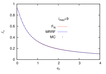
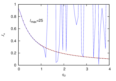
In Figs. 2 and 3, in (44) is
plotted as a function of the spatial frequency . The result is
compared with Monte Carlo simulation and
the method of rotated reference frames.
In Monte Carlo simulation particles were used. To obtain Monte Carlo
simulation for structured illumination, Fourier transform was
performed to results from Monte Carlo simulation for the delta-function
source [35]. Monte Carlo simulation assumed the Henyey-Greenstein
model for the scattering phase function. The method of rotated
reference frames for structured illumination [33, 35]
is summarized in A.
The scattering asymmetry parameter
in Fig. 2 and in Fig. 3.
We set . For both the method and the method of
rotated reference frames we consider and .
In Fig. 2, the three methods agree reasonably well for
. When we increase aiming at more accuracy,
however, from the method of rotated reference frames becomes unstable.
Note that in this case scattering is almost isotropic and discrete
eigenvalues are rather close to . Hence we have
(see (30))
for relatively small .
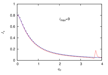
In Fig. 3, the result from the 3D method has a jump near
for because this is not sufficiently
large in this case. A smooth curve is obtained if large enough
is used as shown in the right panel of Fig. 3 for .
Figure 2:
The exitance (44) is plotted against for
, , and . The unit of length is
. For the method and the method of rotated reference frames
(MRRF) we set (Left) and (Right) .
Figure 3:
The exitance (44) is plotted against for
, , and . The unit of length is
. For the method and the method of rotated reference frames
(MRRF) we set (Left) and (Right) .
5 Concluding remarks
The method is similar to the method of rotated reference frames in the
sense that spherical-harmonic expansion is used. However,
in the method, there is no need of expanding singular eigenfunctions.
The extension of the method in the half space to the slab geometry
is straight forward. In the slab geometry, in addition to conditions such as
(4) for one plane at , we have another set of conditions
that corresponds to the other plane. Once the specific intensity on the
boundary is obtained, it is also possible to compute the specific intensity
inside the medium for the half space geometry and the slab geometry
[51].
The author learned the method at the 23rd International Conference
on Transport Theory (September 2013, Santa Fe, New Mexico). He is grateful
to C. E. Siewert and J. C. Schotland for fruitful discussion on collision
expansion.
Monte Carlo simulation was performed using the Monte Carlo solver MC
developed by V. A. Markel.
Appendix A Structured illumination with the method of rotated reference frames
In this section we solve (1) with the method of rotated reference
frames [33, 35]. We consider structured illumination and assume
the source term (39) with (40).
We write the eigenvector of the matrix in (18) corresponding
to the eigenvalue as (). Note that and depend on . In the
method of rotated reference frames, we write the specific intensity as
a superposition of and [41, 48], where
In the half space , the specific intensity is given by
where stands for the sum over all positive eigenvalues of
. From the boundary conditions we obtain
Here are solutions to
where
and
Here,
That is,
where
The hemispheric flux is obtained as
(45)
where we used for
. The expression (45) is used for Figs. 2
and 3.
Appendix B Analytically continued Wigner -matrices
To compute the analytically continued Wigner -matrices we use
a pyramid scheme with recurrence relations [3]. We begin with
, , ,
, and :
Let us we increase iteratively up to . For each value of
, we first compute ()
according to
We obtain and as
and as
With the relation
we have (). Other functions
are obtained by using the symmetry properties
References
References
[1]
Barichello L B, Garcia R D M and Seeder C E 1998
A spherical-harmonics solution for radiative-transfer problems with
reflecting boundaries and internal sources
J. Quant. Spec. Rad. Trans.60 247–260
[2]
Benoist P and Kavenoky A 1968
A new method of approximation of the Boltzmann equation
Nucl. Sci. Eng.32 225–232
[3]
Blanco M A, Flórez M, and Bermejo M 1997
Evaluation of the rotation matrices in the basis of real spherical harmonics
J. Mol. Struct.419 19–27
[4]
Case K M 1960
Elementary solutions of the transport equation and their applications
Ann. Phys.9 1–23
[5]
Case K M, De Hoffmann F and Placzek G 1953
Introduction to the Theory of Neutron Diffusion
Vol. 1, (U. S. Government Printing Office, Washington, D. C.)
[6]
Case K M and Zweifel P F 1967
Linear Transport Theory
(Addison-Wesley)
[7]
Chandrasekhar S 1960
Radiative Transfer
(Dover)
[8]
Dede K M 1964
An explicit solution of the one velocity multi-dimensional
Boltzmann-equation in approximation
Nukleonik6 267-271
[9]
Devaux C and Siewert C E 1980
The method for radiative transfer problems without azimuthal symmetry
J. Appl. Math. Phys.31 592–604
[10]
Duderstadt J J and Martin W R 1979
Transport Theory
(John Wiley & Sons)
[11]
Dunn W L and Siewert C E 1985
The searchlight problem in radiation transport. some analytical and computational results
Z. Ang. Math. Phys.36 581–595
[12]
Grandjean P and Siewert C E 1979
The method in neutron-transport theory. Part II: Applications and
numerical results
Nucl. Sci. Eng.69 161–168
[13]
Garcia R D M 1985
A review of the Facile () method in particle transport theory
Trans. Theo. Stat. Phys.14 391–435
[14]
Garcia R D M and Siewert C E 1981
Multigroup transport theory. II. Numerical results
Nucl. Sci. Eng.78 315–323
[15]
Garcia R D M and Siewert C E 1982
On the dispersion function in particle transpot theory
J. Appl. Math. Phys.33 801–806
[16]
Garcia R D M and Siewert C E 1985
Benchmark results in radiative transfer
Trans. Theo. Stat. Phys.14 437–483
[17]
Garcia R D M and Siewert C E 1989
On discrete spectrum calculations in radiative transfer
J. Quant. Spec. Rad. Trans.42 385–394
[18]
Garcia R D M and Siewert C E 1990
On computing the Chandrasekhar polynomials in high order and high degree
J. Quant. Spec. Rad. Trans.43 201–205
[19]
Garcia R D M and Siewert C E 1992
Improvements in the method for radiative transfer calculations in
clouds
Proceedings of the 11-th International Conference on Clouds and
Precipitation2 813–816
[20]
Garcia R D M and Siewert C E 1998
The method in atmospheric radiative transfer
Int. J. Eng. Sci.36 1623–1649
[21]
Golub G H and Welsch J H 1969
Calculation of Gauss Quadrature Rules
Math. Comp.23 221–230
[22]
Henyey L G and Greenstein J L 1941
Diffuse Radiation in the Galaxy
Astrophys. J.93 70–83
[23]
Kavenoky A 1978
The method of solving the transport equation: Application to plane
geometry
Nucl. Sci. Eng.65 209–225
[24]
Kobayashi K 1977
Spherical harmonics solutions of multi-dimensional neutron transport equation
by finite fourier transformation
J. Nucl. Sci. Tech.14 489-501
[25]
Larsen E W and Habetler G J 1973
A functional-analytic derivation of Case’s full and half-range formulas
Comm. Pure Appl. Math.26 525–537
[26]
Larsen E W 1974
A functional-analytic approach to the steady, one-speed neutron transport
equation with anisotropic scattering
Comm. Pure Appl. Math.27 523–545
[27]
Larsen E W 1975
Solution of neutron transport problem in
Comm. Pure Appl. Math.28 729–746
[28]
Larsen E W, Sancaktar S and Zweifel P F 1975
Extension of the Case formulas to . Application to half and full
space problems
J. Math. Phys.16 1117–1121
[29]
Larsen E W 1982
On a singular integral equation arising in the method
Trans. Theo. Stat. Phys.11 97–103
[30]
Liemert A and Kienle A 2011
Radiative transfer in two-dimensional infinitely extended scattering media
J. Phys. A: Math. Theor.44 505206
[31]
Liemert A and Kienle A 2012
Analytical approach for solving the radiative transfer equation in
two-dimensional layered media
J. Quant. Spec. Rad. Trans.113 559–564
[32]
Liemert A and Kienle A 2012
Infinite space Green’s function of the time-dependent radiative transfer
equation
Biomed. Opt. Exp.3 543–551
[33]
Liemert A and Kienle A 2012
Light transport in three-dimensional semi-infinite scattering media
J. Opt. Soc. Am. A29 1475–1481
[34]
Liemert A and Kienle A 2012
Green’s function of the time-dependent radiative transport equation
in terms of rotated spherical harmonics
Phys. Rev. E86 036603
[35]
Liemert A and Kienle A 2012
Spatially modulated light source obliquely incident
on a semi-infinite scattering medium
Opt. Lett.37 4158–4160
[36]
Liemer A and Kienle A 2013
Exact and efficient solution of the radiative transport equation for the
semi-infinite medium
Sci. Rep.3 2018
[37]
Liemer A and Kienle A 2013
The line source problem in anisotropic neutron transport with internal
reflection
Ann. Nucl. Ene.60 206–209
[38]
Liemer A and Kienle A 2013
Two-dimensional radiative transfer due to curved Dirac delta line sources
Waves in Random and Complex Media23 461–474
[39]
Liemer A and Kienle A 2014
Explicit solutions of the radiative transport equation in the
approximation
Med. Phys.41 111916
[40]
Lukic V, Markel V A and Schotland J C 2009
Optical tomography with structured illumination
Opt. Lett.34 983–985
[41]
Machida M, Panasyuk G, Schotland J C and Markel V A 2010
The Green’s function for the radiative transport equation in the slab geometry
J. Phys. A: Math. Theor.43 065402
[42]
Machida M 2014
Singular eigenfunctions for the three-dimensional radiative transport equation
J. Opt. Soc. Am. A31 67–74
[43]
Markel V A 2004
Modified spherical harmonics method for solving the radiative transport
equation
Waves Random Media14 L13–9
[44]
McCormick N J and Kuščer I 1965
Half-space neutron transport with linearly anisotropic scattering
J. Math. Phys.6 1939–1945
[45]
McCormick N J and Kuščer I 1966
Bi-orthogonality relations for solving half-space transport problems
J. Math. Phys.7 2036–2045
[46]
McCormick N J and Sanchez R 1981
Inverse problem transport calculations for anisotropic scattering coefficients
J. Math. Phys.22 199–208
[47]
Mika J R 1961
Neutron transport with anisotropic scattering
Nucl. Sci. Eng.11 415–427
[48]
Panasyuk G, Schotland J C and Markel V A 2006
Radiative transport equation in rotated reference frames
J. Phys. A: Math. Gen.39 115–137
[49]
Sanchez R and McCormick N J 1982
A review of neutron transport approximations
Nucl. Sci. Eng.80 481–535
[50]
Schotland J C and Markel V A 2007
Fourier-Laplace structure of the inverse scattering problem for the
radiative transport equation
Inv. Prob. Imag.1 181–188
[51]
Siewert C E 1978
The method for solving radiative-transfer problems in plane geometry
Astrophys. Space Sci.58 131–137
[52]
Siewert C E and Benoist P 1979
The method in neutron-transport theory. Part I: Theory and applications
Nucl. Sci. Eng.69 156–160
[53]
Siewert C E and Dunn W L 1983
Radiation transport in plane-parallel media with non-uniform surface illumination
Z. Ang. Math. Phys.34 627–641
[54]
Siewert C E and McCormick N J 1997
Some identities for Chandrasekhar polynomials
J. Quant. Spectrosc. Radiat. Transfer57 399–404
[55]
Williams M M R 1982
The three-dimensional transport equation with applications to energy deposition and reflection
J. Phys. A: Math. Gen.15 965–983
[56]
Xu H and Patterson M S 2006
Application of the modified spherical harmonics method to some problems
in biomedical optics
Phys. Med. Biol.51 N247–N251
[57]
Xu H and Patterson M S 2006
Determination of the optical properties of tissue-simulating phantoms from
interstitial frequency domain measurements of relative fluence and
phase difference
Opt. Exp.14 6485–6501