Virtual reality based approach to protein
heavy-atom structure reconstruction

Abstract

Background A commonly recurring problem in structural protein studies, is the determination of all heavy atom positions from the knowledge of the central $\alpha$-carbon coordinates.

Results We employ advances in virtual reality to address the problem. The outcome is a 3D visualisation based technique where all the heavy backbone and side chain atoms are treated on equal footing, in terms of the C_α coordinates. Each heavy atom can be visualised on the surfaces of the different two-spheres, that are centered at the other heavy backbone and side chain atoms. In particular, the rotamers are visible as clusters which display strong dependence on the underlying backbone secondary structure.

Conclusions Our method easily detects those atoms in a crystallographic protein structure which have been been likely misplaced. Our approach forms a basis for the development of a new generation, visualisation based side chain construction, validation and refinement tools. The heavy atom positions are identified in a manner which accounts for the secondary structure environment, leading to improved accuracy over existing methods.

Keywords: Side chain reconstruction, C_α trace problem, rotamers, protein visualisation

Protein structure validation methods like MolProbity Chen-2010 and Procheck Laskowski-1993 help crystallographers to find and fix potential problems that are incurred during fitting and refinement. These methods are commonly based on a priori chemical knowledge and utilize various well tested and broadly accepted stereochemical paradigms. Likewise, template based structure prediction and analysis packages Qu-2009 and molecular dynamics force fields Freddolino-2010 are customarily built on such paradigms. Among these, the Ramachandran map Ramachandran-1963 , Carugo-2013 has a central rôle. It is widely deployed both to various analyzes of the protein structures, and as a tool in protein visualization. The Ramachandran map describes the statistical distribution of the two dihedral angles $\phi$ and $\psi$ that are adjacent to the C_α carbons along the protein backbone. A comparison between the observed values of the individual dihedrals in a given protein with the statistical distribution of the Ramachandran map is an appraised method to validate the backbone geometry.

In the case of side chain atoms, visual analysis methods alike the Ramachandran map have been introduced. For example, the Janin map Janin-1978 can be used to compare observed side chain dihedrals such as $\mathcal{X}_{1}$ and $\mathcal{X}_{2}$ in a given protein, against their statistical distribution, in a manner which is analogous to the Ramachandran map. Crystallographic refinement and validation programs like Phenix Adams-2010 , Refmac Murshudov-1997 and others, often utilize the statistical data obtained from the Engh and Huber library Engh-1991 , Engh-2001 . This library is built using small molecular structures that have been determined with a very high resolution. At the level of entire proteins, side chain restraints are commonly derived from analysis of high resolution crystallographic structures Ponder-1987 , Dunbrack-2002 in Protein Data Bank (PDB) Berman-2000 . A backbone independent rotamer library Lovell-2000 makes no reference to backbone conformation. But the possibility that the side-chain rotamer population depends on the local protein backbone conformation, was considered already by Chandrasekaran and Ramachandran Chandrasekaran-1970 . Subsequently both secondary structure dependent Schrauber-1993 , see also Janin-1978 and Lovell-2000 , and backbone dependent rotamer libraries Dunbrack-1993 , Shapovalov-2011 have been developed. The information content in the secondary structure dependent libraries and the backbone independent libraries essentially coincide Dunbrack-2002 . Both kind of libraries are used extensively during crystallographic protein structure model building and refinement. But for the prediction of side-chain conformations for example in the case of homology modeling and protein design, there can be an advantage to use the more revealing backbone dependent rotamer libraries.

In x-ray crystallographical protein structure experiments, the skeletonization of the electron density map is a common technique to interpret the data and to build the initial model Jones-1991 . The C_α atoms are located at the branch points between the backbone and the side chain, and as such they are subject to relatively stringent stereochemical constraints; this is the reason why the model building often starts with the initial identification of the skeletal C_α trace. The central rôle of the C_α atoms is widely exploited in structural classification schemes such as CATH Sillitoe-2013 and SCOP Murzin-1995 , in various threading Roy-2010 and homology Schwede-2003 modeling techniques Zhang-2009 , in de novo approaches Dill-2007 , and in the development of coarse grained energy functions for folding prediction Scheraga-2007 . As a consequence the so-called C_α-trace problem has become the subject of extensive investigations Holm-1991 ; DePristo-2003 ; Lovell-2003 ; Rotkiewicz-2008 ; Li-2009 . The resolution of the problem would consist of an accurate main chain and/or all-atom model of the folded protein from the knowledge of the positions of the central C_α atoms only. Both knowledge-based approaches such and MAXSPROUT Holm-1991 and de novo methods including PULCHRA Rotkiewicz-2008 and REMO Li-2009 have been developed, to try and resolve the C_α trace problem. In the case of the backbone atoms, the geometric algorithm introduced by Purisima and Scheraga Purisima-1984 , or some variant thereof, is commonly utilized in these approaches. For the side chain atoms, most approaches to the C_α trace problem rely either on a statistical or on a conformer rotamer library in combination with steric constraints, complemented by an analysis which is based on diverse scoring functions. For the final fine-tuning of the model, all-atom molecular dynamics simulations can also be utilized.

In the present article we introduce and develop new generation visualization techniques that we hope will become a beneficial component in protein structure analysis, refinement and validation. In line with the concept of the C_α trace problem we deploy only a geometry that is determined solely in terms of the C_α coordinates. The output we aim at, is a 3D ”what-you-see-is-what-you-have” type visual map of the statistically preferred all-atom model, calculable in terms of the C_α coordinates. As such, our approach should have value for example during the construction and validation of the initial backbone and all-atom models of a crystallographic protein structure.

Our approach is based on developments in three dimensional visualization and virtual reality, that have taken place mainly after the Ramachandran map was introduced. In lieu of the backbone dihedral angles that appear as coordinates in the Ramachandran map and correspond to a toroidal topology, we employ the geometry of virtual two-spheres that surround each heavy atom. We visually describe all the higher level heavy backbone and side chain atoms on the surface of the sphere, level-by-level along the backbone and side chains, exactly in the manner how they are seen by an imaginary, geometrically determined and C_α based miniature observer who roller-coasts along the backbone and climbs up the side chains, while proceeding from one C_α atom to the next. At the location of each C_α our virtual observer orients herself consistently according to the purely geometrically determined C_α based discrete Frenet frames Hu-2011 ; Lundgren-2012a . Thus the visualization depends only on the C_α coordinates, there is no reference to the other atoms in the initialization of the construction. The other atoms - including subsequent C_α atoms along the backbone chain - are all mapped on the surface of a sphere that surrounds the observer, as if these atoms were stars in the sky.

At each C_α atom, the construction proceeds along the ensuing side chain, until the position of all heavy atoms have been determined. As such our maps provide a purely geometric and equitable, direct visual information on the statistically expected all-atom structure in a given protein.

The method we describe in this article, can form a basis for the future development of a novel approach to the C_α trace problem. Unlike the existing approaches such as MAXSPROUT Holm-1991 , PULCHRA Rotkiewicz-2008 and REMO Li-2009 the method we envision accounts for the secondary structure dependence in the heavy atom positions, which we here reveal. A secondary-structure dependent method to resolve the C_α trace problem should lead to an improved accuracy in the heavy atom positions, in terms of the C_α coordinates. The present article is a proof-of-concept.

I Method and Results

I.1 C_α based Frenet frames

Let $\mathbf{r}_{i}$ ($i=1,...,N$) be the coordinates of the C_α atoms. The counting starts from the N terminus. At each $\mathbf{r}_{i}$ we introduce the orthonormal, right-handed, discrete Frenet frame ($\mathbf{t}_{i},\mathbf{n}_{i},\mathbf{b}_{i}$) Hu-2011 . As shown in figure 1

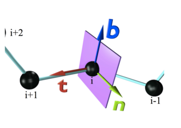
Figure 1: (Color online) Discrete Frenet frame vectors (1), (2) and (3).

the tangent vector $\mathbf{t}$ points from the center of the $i^{th}$ central carbon towards the center of the $(i+1)^{st}$ central carbon,

$$\mathbf{t}_{i}\ =\ \frac{\mathbf{r}_{i+1}-\mathbf{r}_{i}}{|\mathbf{r}_{i+1}-\mathbf{r}_{i}|}$$ (1)

The binormal vector is

$$\hskip-12.80365pt\mathbf{b}_{i}\ =\ \frac{\mathbf{t}_{i-1}\times\mathbf{t}_{i}}{|\mathbf{t}_{i-1}\times\mathbf{t}_{i}|}$$ (2)

The normal vector is

$$\hskip-25.6073pt\mathbf{n}_{i}\ =\ \mathbf{b}_{i}\times\mathbf{t}_{i}$$ (3)

We also introduce the virtual C_α backbone bond ($\kappa$) and torsion ($\tau$) angles, shown in figure 2.

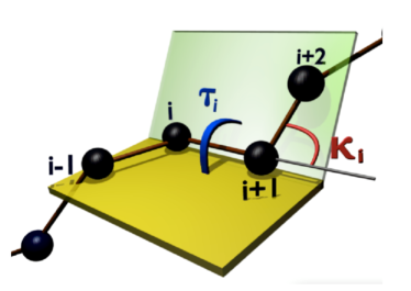
Figure 2: (Color online) Geometry of bond ($\kappa_{i}$) and torsion ($\tau_{i}$) angles (4) and (5).

These angles are computed as follows,

$$\cos\kappa_{i+1}\ =\ \mathbf{t}_{i+1}\cdot\mathbf{t}_{i}$$ (4)

$$\cos\tau_{i+1}\ =\ \mathbf{b}_{i+1}\cdot\mathbf{b}_{i}$$ (5)

We identify the bond angle $\kappa\in[0,\pi]$ with the latitude angle of a two-sphere which is centered at the C_α carbon. We orient the sphere so that the north-pole where $\kappa=0$ is in the direction of $\mathbf{t}$. The torsion angle $\tau\in[-\pi,\pi)$ is the longitudinal angle. It is defined so that $\tau=0$ on the great circle that passes both through the north pole and through the tip of the normal vector $\mathbf{n}$. The longitude angle increases towards the counterclockwise direction around the vector $\mathbf{t}$. Additional visual gain can be obtained, by stereographic projection of the sphere onto the plane. The standard stereographic projection from the south-pole of the sphere to the plane with coordinates ($x,y$) is given by

$$x+iy\ \equiv\ \sqrt{x^{2}+y^{2}}\,e^{i\tau}\ =\ \tan\left(\kappa/2\right)\,e^{i\tau}$$ (6)

This maps the north-pole where $\kappa=0$ to the origin ($x,y$)$=$($0,0$). The south-pole where $\kappa=\pi$ is sent to infinity; see figure 3

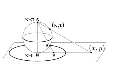
Figure 3: (Color online) Geometry of bond ($\kappa_{i}$) and torsion ($\tau_{i}$) angles (4) and (5).

The visual effects can be further enhanced by sending

$$\kappa\ \to\ f(\kappa)$$ (7)

where $f(\kappa)$ is a properly chosen function of the latitude angle $\kappa$. Various different choices of $f(\kappa)$ will be considered in the sequel.

I.2 The C_α map

We first describe, how to visually characterize the C_α trace in terms of the C_α based Frenet frames (1)-(3). We introduce the concept of a virtual miniature observer who roller-coasts the backbone by moving between the C_α atoms. At the location of each C_α the observer has an orientation that is determined by the Frenet frames (1)-(3). The base of the $i^{th}$ tangent vector $\mathbf{t}_{i}$ is at the position $\mathbf{r}_{i}$. The tip of $\mathbf{t}_{i}$ is a point on the surface of the sphere ($\kappa,\tau$) that surrounds the observer; it points towards the north-pole. The vectors $\mathbf{n}_{i}$ and $\mathbf{b}_{i}$ determine the orientation of the sphere, these vectors define a frame on the normal plane to the backbone trajectory, as shown in figure 1. The observer uses the sphere to construct a map of the various atoms in the protein chain. She identifies them as points on the surface of the two-sphere that surrounds her, as if the atoms were stars in the sky.

The observer constructs the C_α backbone map as follows Lundgren-2012a . She first translates the center of the sphere from the location of the $i^{th}$ C_α, all the way to the location of the $(i+1)^{th}$ C_α, without introducing any rotation of the sphere, with respect to the $i^{th}$ Frenet frames. She then identifies the direction of $\mathbf{t}_{i+1}$, i.e. the direction towards the site $\mathbf{r}_{i+2}$ to which she proceeds from the next C_α carbon, as a point on the surface of the sphere. This determines the corresponding coordinates ($\kappa_{i},\tau_{i}$). After this, she re-defines her orientation to match the Frenet framing at the $(i+1)^{th}$ central carbon, and proceeds in the same manner. The ensuing map, over the entire backbone, gives an instruction to the observer at each point $\mathbf{r}_{i}$, how to turn at site $\mathbf{r}_{i+1}$, to reach the $(i+2)^{th}$ C_α carbon at the point $\mathbf{r}_{i+2}$.

In figure 4 (top)

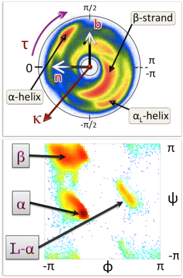
Figure 4: (Color online) Top: The stereographically projected Frenet frame map of backbone C_α atoms, with major secondary structures identified. Also shown is the directions of the Frenet frame normal vector $\mathbf{n}$; the vector $\mathbf{t}$ corresponds to the red circle at the center, and it points away from the viewer. The map is constructed using all PDB structures that have been measured with better than 2.0 Å  resolution. Bottom: Standard Ramachandran map, constructed using our 1.0 Å  resolution PDB subset. Major secondary structures have been identified.

we show the C_α Frenet frame backbone map. It describes the statistical distribution that we obtain when we plot all PDB structures which have been measured with better than 2.0 Å  resolution, and using the stereographic projection (6); for statistical clarity we prefer to use here a more extended subset of PDB, than our canonical 1.0 Å subset, which we shall use in the remainder of the present article. Here the difference is minor.

For our observer, who always fixes her gaze position towards the north-pole of the surrounding two-sphere at each C_α i.e. towards the red dot at the center of the annulus, the color intensity in this map reveals the probability of the direction at position $\mathbf{r}_{i}$, where the observer will turns at the next C_α carbon, when she moves from $\mathbf{r}_{i+1}$ to $\mathbf{r}_{i+2}$. In this way, the map is in a direct visual correspondence with the way how the Frenet frame observer perceives the backbone geometry. We note that the probability distribution concentrates within an annulus, roughly between the latitude angle values $\kappa\sim 1$ and $\kappa\sim 3/2$. The exterior of the annulus is a sterically excluded region while the entire interior is in principle sterically allowed but not occupied in the case of folded proteins. In the figure we identify four major secondary structure regions, according to the PDB classification. These are $\alpha$-helices, $\beta$-strands, left-handed $\alpha$-helices and loops. In this article we will use this rudimentary level PDB classification thorough.

We note that the visualization in figure 4 (top) resembles the Newman projection of stereochemistry: The vector $\mathbf{t}_{i}$ which is denoted by the red dot at the center of the figure, points along the backbone from the promixal C_α at $\mathbf{r}_{i}$ towards the distal C_α at $\mathbf{r}_{i+1}$. This convention will be used thorough the present article.

When we surround C_α with an imaginary two-sphere, with C_α at the origin, we may choose the radius of the sphere to coincide with the (average) covalent bond length value Lundgren-2012a which is 3.8 Å in the case of C_α atoms, excluding the cis-proline . Since the variations in the covalent bond lengths are in general minor, in this article we do not account for deviations in covalent bond lengths from their ideal values.

For comparison, we also show in figure 4 (bottom) the standard Ramachandran map. The sterically allowed and excluded regions are now intertwined, while the allowed regions are more localized than in figure 4 (top). We point out that the map in figure 4 (top) provides non-local information on the backbone geometry, it extends over several peptide units, and tells the miniature observer where the backbone turns at the next C_α. As such it goes beyond the regime of the Ramachandran map, which is localized to a single C_α carbon and does not provide direct information how the backbone proceeds: The two Ramachandran angles $\phi$ and $\psi$ are dihedrals for a given C_α, around the N-C_α and C_α-C covalent bonds. These angles to not furnish information about neighboring peptide groups.

I.3 Backbone heavy atoms

Consider our imaginary miniature observer, located at the position of a C_α atom and oriented according to the discrete Frenet frames. She observes and records the backbone heavy atoms N, C and the side-chain C_β that are covalently bonded to a given C_α, and the O in the peptide plane that precedes C_α. In figures 5 a)-d)

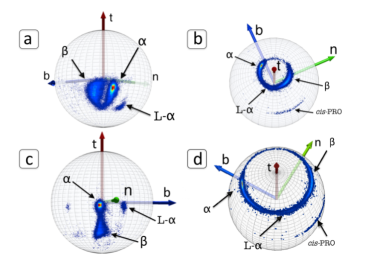
Figure 5: (Color online) a) Distribution of C_β atoms in the C_α centered Frenet frames in PDB structures that have been measured with better than 1.0 Å resolution. The three major structures $\alpha$-helices, $\beta$-strands and left-handed $\alpha$- helices have been marked, following their identification in PDB. b) Same as a) but for backbone C atoms. Note that C atoms that precede a $cis$-proline are clearly identifiable. c) Same as a) and b) but for backbone N atoms. d) Same as a), b) and c) but for backbone O atoms. As in b) the atoms preceding a $cis$-proline are clearly identifiable.

we show the ensuing density distributions, on the surface of the C_α centered sphere. These figures are constructed from all the PDB entries that have been measured using diffraction data with better than 1.0 Å resolution.

We note clear rotamer structures: The C_β, C, N and O atoms are each localized, and in a manner that depends on the underlying secondary structure Lundgren-2012b . Both in the case of C_β and N, the left-handed $\alpha$ region (L-$\alpha$) is a distinct rotamer which is detached from the rest. In the case of C and O, the L-$\alpha$ region is more connected with the other regions. But for C and O, the region for residues before cis-prolines becomes detached from the rest. In the case of C and C_β we do not observe any similar isolated and localized cis-proline rotamer.

The C and O rotamers concentrate on a circular region, with essentially constant latitude angle with respect to the Frenet frame tangent vector; for the O distribution, the latitude is larger. The N rotamers form a narrow strip in the longitudinal direction, while the map for C_β rotamers form a shape that resembles a horse shoe.

For comparison, in figure 6

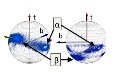
Figure 6: (Color online) Distribution of C_β atoms (left) and backbone N atoms (right) in the frames of REMO Li-2009 .

we visualize the C_β and N distributions in the coordinate system that is utilized in REMO Li-2009 . The secondary structures can be identified, but the rotamers are clearly more delocalized than in the case of the Frenet frame map, shown in figure 5 a) and c). This delocalization persists in the case of backbone C and O atoms (not shown). Similarly, we have found that in the case of the coordinate system of PULCHRA Rotkiewicz-2008 , the rotamers are similarly clearly more delocalized than in the Frenet frames (not shown).

One may argue that the stronger the localization of rotamers, the more precise will structure analysis, prediction and validation become. From this perspective, the Frenet frames have an advantage over the frames used e.g. in PULCHRA and REMO.

The N, C and C_β atoms form the covalently bonded heavy-atom corners of the C_α centered $sp3$-hybridized tetrahedron. We consider the three bond angles

$$\vartheta_{\rm NC}~{}\simeq~{}{\rm N-C}_{\alpha}-{\rm C}~{}$$ (8)

$$\vartheta_{{\rm N}\beta}~{}\simeq~{}{\rm N-C}_{\alpha}-{\rm C}_{\beta}$$ (9)

$$\vartheta_{\beta\rm C}~{}\simeq~{}{\rm C}_{\beta}-{\rm C}_{\alpha}-{\rm C}$$ (10)

The $\vartheta_{\rm NC}$ angle relates to the backbone only, while the definition of the other two involves the side chain C_β. In figure 7

Figure 7: (Color online) Distribution of the three bond angles (8)-(10), according to secondary structures. Blue are $\alpha$-helices, red are $\beta$-strands and yellow are loops; the small (yellow) peak in N-C_α-C_β with angle around 103^o is due to prolines. See Table 1 for the average values for $\alpha$-helices, $\beta$-strands and loops in figure a). See also Table 2 for the average values in figures a), b) and c) with no regard to secondary structure. Finally, see Table 3 for the average values.

we show the distribution of the three tetrahedral bond angles (8)-(10) in our PDB data set. We find that in the case of the two side chain C_β related angles $\vartheta_{{\rm N}\beta}$ and $\vartheta_{\beta\rm C}$, the distribution has a single peak which is compatible with ideal values; the isolated small peak in figure 7 b) is due to $cis$-prolines. But in the case of the backbone-only specific angle $\vartheta_{\rm NC}$ we find that in our data set this is not the case. The PDB data set we use and display in figure 7 a) shows, that there is a correlation between the $\vartheta_{\rm NC}$ distribution and the backbone secondary structure. See also Table 1.

Structure	$\vartheta_{{\rm NC}}$
Helix	111.5  $\pm$ 1.7
Strand	109.1  $\pm$ 2.0
Loop	111.0  $\pm$ 2.5

Table 1: Average values of the angle $\vartheta_{\rm NC}$ separately for $\alpha$-helices, $\beta$-strands and loops in figure 7 a) with one-$\sigma$ standard deviations.

We note that in protein structure validation all three angles (8)-(10) are commonly presumed to assume the ideal values, shown in Table 3.

Angle	$\vartheta_{{\rm NC}}$	$\vartheta_{{\rm C}\beta}$	$\vartheta_{\beta{\rm N}}$
All	110.7  $\pm$ 2.3	110.5  $\pm$ 2.0	110.3  $\pm$ 2.4
PRO	112.6  $\pm$ 2.2	111.3  $\pm$ 1.7	103.2  $\pm$ 1.1
rest	110.6  $\pm$ 2.3	110.4  $\pm$ 2.0	110.7  $\pm$ 1.7

Table 2: Average values of the angles in figures 7 computed from our PDB data set, without subdivision according to secondary structure, and with one-$\sigma$ standard deviations. See also Table 3.

Residue	EH-1	EH-2	AK	TV
$\vartheta_{{\rm NC}}$(PRO)		112.1 $\pm$ 2.6		112.8 $\pm$ 3.0
$\vartheta_{{\rm NC}}$(REST)	110.5	111.0 $\pm$ 2.7	110.4 $\pm$ 3.3	111.0 $\pm$ 3.0
$\vartheta_{{\rm C}\beta}$	110.1		110.1 $\pm$ 2.9
$\vartheta_{\beta{\rm N}}$	111.2		110.1 $\pm$ 2.8

Table 3: Some average values of the angles in figure 7 reported by various authors, together with their one-$\sigma$ standard deviations.

For example, the deviation of the C_β atom from its ideal position is among the validation criteria in MolProbity Chen-2010 , that uses it to identify potential backbone distortions around C_α. But several authors Lundgren-2012b -Touw have pointed out that certain variation in the values of the $\tau_{\rm NC}$ can be expected, and is in fact present in PDB data. Accordingly, the protein backbone geometry does not obey the single ideal value paradigm. Since this paradigm motivates the applicability of small molecule libraries such as the Engh and Huber library Engh-1991 , Engh-2001 , there is a good case to be made in favor of using the PDB based libraries Lovell-2000 , Dunbrack-1993 , Shapovalov-2011 in the case of proteins.

We remind that $\vartheta_{\rm NC}$ pertains to the two peptide planes that are connected by the C_α. The Ramachandran angles ($\phi,\psi$) are the adjacent dihedrals, but unlike $\vartheta_{\rm NC}$ they are specific to a single peptide plane; the Ramachandran angles describe the twisting of the ensuing peptide plane. If the internal structure of the peptide planes is assumed to be rigid, the flexibility in the bond angle $\vartheta_{\rm NC}$ remains the only coordinate that can contribute to the bending of the backbone. Consequently a systematic secondary structure dependence, as displayed in figure 7, is to be expected. It could be that the lack of any observable secondary structure dependence in $\vartheta_{{\rm N}\beta}$ and $\vartheta_{\beta\rm C}$ suggests that existing validation methods distribute all refinement tension on $\vartheta_{\rm NC}$.

I.4 C_β atoms

The side chains are connected to the C_α backbone by the covalent bond between C_α and C_β. Consequently the precision, and high level of localization in the C_β map becomes pivotal for the construction of accurate higher level side chain maps.

I.4.1 C_β at termini:

We have analyzed those C_β atoms that are located in the immediate proximity of the N and the C termini in the PDB data. For this, we have considered the first two C_β atoms starting from the N terminus, and the last two C_β atoms that are before the C terminus. Note that in the data that describes a crystallographic PDB structure, these do not need to correspond to the actual biological termini of the biological protein. In case the termini of the biological protein can not be crystallized, the PDB data describes the first two residues after the N terminus reps. the last two residues prior to the C terminus that can be crystallized. Here we consider the termini, as they appear in the PDB data.

Recall, that the termini are commonly located on the surface of the protein. As such, they are accessible to solvent and quite often oppositely charged. It is frequently presumed that the termini are unstructured and highly flexible. They are normally not given any regular secondary structure assignment in PDB. But the figure 8 shows that in the C_α Frenet frames the orientations of the two terminal C_β atoms

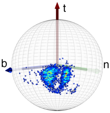
Figure 8: (Color online) The distribution of C_β directions in the first two and last two residues along PDB structures that have been measured using diffraction data with better than 1.0 Å resolution. There is no visible difference to the Figure 3 a). In particular, there are very few clear outliers, and they are located mainly in the region left of the main region.

are highly regular. Their positions on the surface of the C_α centered sphere are fully in line with that of all the other C_β atoms, as shown in figure 5 a). In particular, there are very few outliers. Moreover, the few outliers are (mainly) concentrated in a small region which is located towards the left from the $\beta$-stranded structures.

I.4.2 C_β and proline:

In figure 9

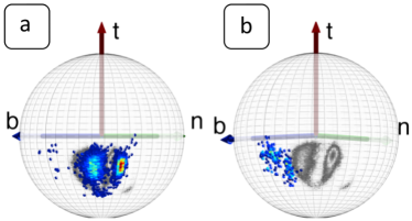
Figure 9: (Color online)The distribution of C_β in prolines. Figure a) is $trans$-PRO and figure b) is $cis$-PRO. The grey background is given by Figure 5 a).

we compare the individual proline contributions in our data set with the C_β background in figure 5 a). In figure 9 a) we show the $trans$-proline, and in figure 9 b) we show the $cis$-proline. The $trans$-proline has a very good match with the background. There are very few outliers. These are predominantly located in the same region as in figure 8, towards the left from the main distribution i.e. towards increasing longitude. We observe that all the $cis$-proline are located outside of the main C_β distribution, towards the increasing longitude from the main distribution.

In figures 10 a)-d)

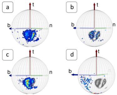
Figure 10: (Color online) The distribution of C_β atoms immediately after and right before a proline. The grey-scaled background is determined by the high-density region of figure 5 a). In figure a) immediately after $trans$-PRO and in figure b) immediately after $cis$-PRO. In figure c) right before $trans$-PRO and in figure d) right before $cis$-PRO.

we display the C_β carbons that are located either immediately after or right before a proline. We observe the following:

In figure 10 a) we have the C_β that are immediately after the $trans$-proline. The distribution matches the background, with very few outliers that are located mostly in the same region as in figures 8, 9 i.e. towards increasing longitude. But there is a very high density peak in the figure, that overlaps with the $\alpha$-helical region: We remind that proline is commonly found right before the first residue in a helix.

In figure 10 b) we display those C_β atoms which are immediately after the $cis$-proline. There is again a good match with the background. But unlike in figure 10 a) we also observe a shift towards increasing longitude. in particular, the high density region now coincides with the $\beta$-stranded region in the background. There are very few outliers, again mainly towards increasing longitude.

In figure 10 c) we have those C_β that are right before a $trans$-proline. There is a clear match with the background distribution. But there are relatively few entries in the $\alpha$-helical position: It is known that helices rarely end in a proline. The intensity is very large in the loop region that overlaps the $\beta$-stranded region. There are also a few outliers. Again, the outliers are mainly located in the region towards increasing longitude.

In Figure 10 d) we show the C_β distribution for residues that are right before a $cis$-proline. There are no entries in the background region of figure 5 a). The distribution is almost fully located in the previously observed outlier region, towards the left of the background in the figure. In addition, we observe an extension of this region towards increasing latitude, reaching all the way to the south-pole.

Finally, we recall that in figure 5 b) the region that corresponds to the effect of $cis$-prolines in the preceding C rotamer, is clearly visible. But in the case of C_β and N atoms, we do not observe any similar high density isolated $cis$-region. Consequently the question arises whether the structure of the C_α centered covalent tetrahedron is deformed:

In figure 11 we show the distribution of the three angles;

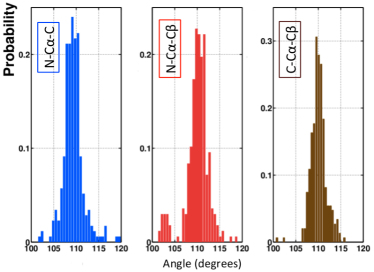
Figure 11: (Color online) Distribution of the three heavy atom related angles (in degrees) in the C_α centered covalent tetrahedron, in the case of $cis$-proline. The numerical average values together with the one standard deviations are given in Table 4.

see also Table 4.

Table 4: Average values of the angles in figure 11, together with their one-$\sigma$ standard deviations.

Angle	$\vartheta_{{\rm NC}}$	$\vartheta_{{\rm C}\beta}$	$\vartheta_{\beta{\rm N}}$
average	109.3 $\pm$ 2.2	110.1 $\pm$ 1.8	110.0 $\pm$ 2.6

We observe a small deviation in the angle N-C_α-C. In comparison to proline values in Table 2, the value we find in our data set is smaller.

I.4.3 C_β and histidine:

As another example, in figures 12

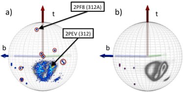
Figure 12: (Color online) Figure a) shows C_β distribution of histidine. Some apparent outliers have been encircled, as examples. Residue number 312A in the PDB entry 2PF8 has been identified, together with 312 in the same protein 2PEV. Figure b) shows the subset of those HIS that precede a $cis$-PRO, there are five in our data set.

we display the C_β distribution in the case of histidine. The figure 12 a) shows that there is a very good match with the statistical background distribution. There are only a few apparent outliers. Some of them have been encircled, as examples. One of the apparent outliers corresponds to the residue number 312 (HIS) in the PDB entry 2PF8. The latitude is anomalously small. The residue is located relatively close to the C-terminal of the backbone. But comparison with figure 8 proposes that this is not the cause for its anomalous latitude position. The PDB file of 2PF8 reveals that this C_β atom has two alternative positions. The one we have displayed (312A) is in an atypical position. The other is not. This is also supported by the Frenet frame orientation of the same C_β atom 312 in a different PDB entry of the same protein, with code 2PEV. The C_β atom 312 of 2PEV is located in the highly populated $\alpha$-helical region. The reason for the atypical positioning of 312A in 2PF8 remains to be understood.

In figure 12 b) we plot those HIS that precede a $cis$-PRO i.e. are also present in Figure 10 d). There are five such entries in HIS. They are all located in the rotamer that appears to be statistically favored in figure 10 d).

I.5 Level-$\gamma$ rotamers

I.5.1 Standard rotamers:

We proceed upwards along the side-chain, to the level-$\gamma$ heavy atoms that are covalently bonded to C_β. Conventionally, these atoms are described by the side-chain dihedral angle $\mathcal{X}_{1}$. This angle is determined by the three covalently bonded heavy atoms C_α, C_β and N. The angle $\mathcal{X}_{1}$ determines the dihedral orientation of the level-$\gamma$ carbon atom, in terms of these three atoms.

We remind that ALA and GLY do not contain any level-$\gamma$ atoms. In the case of ILE and VAL we have two C_γ while in the case of CYS there is a S_γ atom.

We first define a $\mathcal{X}1$-framing, where the rotamer angle $\mathcal{X}_{1}$ appears as a dihedral coordinate. For this we introduce the following C_α based orthonormal triplet

$$\hskip-150.79968pt\mathbf{t}_{\mathcal{X}1}\ =\ \frac{\mathbf{r}_{\beta}-\mathbf{r}_{\alpha}}{|\mathbf{r}_{\beta}-\mathbf{r}_{\alpha}|}$$ (11)

$$\mathbf{n}_{\mathcal{X}1}\ =\ \frac{\mathbf{s}-\mathbf{t}_{\mathcal{X}1}(\mathbf{s}\cdot\mathbf{t}_{\mathcal{X}1})}{|\,\mathbf{s}-\mathbf{t}_{\mathcal{X}1}(\mathbf{s}\cdot\mathbf{t}_{\mathcal{X}1})\,|}\ \ \ \ \ {\rm where}\ \ \ \ \ \mathbf{s}=\mathbf{r}_{\alpha}-\mathbf{r}_{\rm N}$$ (12)

$$\hskip-156.49014pt\mathbf{b}_{\mathcal{X}1}\ =\ \mathbf{t}_{\mathcal{X}1}\times\mathbf{n}_{\mathcal{X}1}$$ (13)

with $\mathbf{r}_{\alpha}$, $\mathbf{r}_{\beta}$ and $\mathbf{r}_{N}$ the coordinates of the pertinent C_α, C_β and N atoms, respectively. This constitutes our $\mathcal{X}1$-framing, with C_α at the origin. We introduce a sphere around C_α, oriented so that the north-pole is in the direction of $\mathbf{t}_{\mathcal{X}1}$. Now the dihedral $\mathcal{X}_{1}$ coincides with the ensuing longitude angle.

In figures 13 we show the distribution of level-$\gamma$ carbon atoms.

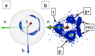
Figure 13: (Color online) a) C_γ atoms in the $\mathcal{X}1$-frames (11)-(13) on the C_α centered two-sphere. b) Stereographic projection of a) using (14). The three rotamers and proline are identified.

The figure 13 a) shows the distribution on the surface of the C_α centered two-sphere. In figure 13 b) we use the stereographic projection (6) with the choice

$$f(\kappa)=\frac{1}{1+\exp\{\kappa^{2}\}}$$ (14)

in equation (7). The three rotamers gauche$\pm$ (g$\pm$) and trans (t) have been identified in this figure. The prolines are also visible, as rotamers. In addition, in figure 13 b) we have a circle that shows the average distance of the data points from the north-pole (origin) on the stereographic plane. A number of apparent outliers are visible in fig. 13 b).

We note that the underlying secondary structure of the backbone is not visible in figures 13. This is a difference between figures 5 and 13, in the former the underlying backbone secondary structure is visible in the density profile.

In figures 14

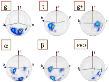
Figure 14: (Color online) Frenet frame view of the level-$\gamma$ carbons, separately for the three rotamer states $g\pm$ and $t$ (top line) and for for $\alpha$-helices, $\beta$-strands and prolines (bottom line).

we show how the C_γ atoms are seen by the observer who is located at the C_α atom, and oriented according to the backbone Frenet frames; these are the frames used in figures 5. Now both the rotamer structure and the various backbone secondary structures are clearly seen.

I.5.2 Secondary structure dependent level-$\gamma$ rotamers:

In the C_α Frenet frame figures 14 the secondary structure dependence is visible. But unlike figure 13 a) the C_α Frenet frame figures 14 lack an apparent symmetry. This complicates the implementation of the stereographic projection, such as the one shown in figure 13 b). We proceed to introduce a new set of frames, that enables us to analyze the secondary structure dependence of the $\gamma$-level atoms in terms of the stereographic projection:

We choose the unit length vector $\mathbf{t}_{\beta}$, to coincide with the unit vector that points from C_α at point $\mathbf{r}_{\alpha}$ towards C_β at point $\mathbf{r}_{\beta}$.

$$\mathbf{t}_{\beta}=\frac{\mathbf{r}_{\beta}-\mathbf{r}_{\alpha}}{|\mathbf{r}_{\beta}-\mathbf{r}_{\alpha}|}$$ (15)

We use the next C_α atom along the backbone, to define the following unit length vector

$$\mathbf{n}_{\beta}=\frac{\mathbf{t}_{\beta}\times\mathbf{t}_{\alpha}}{|\mathbf{t}_{\beta}\times\mathbf{t}_{\alpha}|}$$ (16)

Here $\mathbf{t}_{\alpha}$ is the vector (1). The orthonormal triplet is completed by

$$\mathbf{b}_{\beta}=\mathbf{t}_{\beta}\times\mathbf{n}_{\beta}$$ (17)

We may choose either C_α or C_β to coincide with the origin; the C_α centered coordinate system is the original roller coasting observer while the C_β centered coordinate system corresponds to an observer who has climbed ”one-step-up” along the side chain. We map the level-$\gamma$ atoms on the surface of the pertinent, surrounding two-spheres. In figures 15 a) and b)

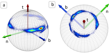
Figure 15: (Color online)The level-$\gamma$ atoms as seen in the coordinates (15)-(16). In a) the origin coincides with the C_α atom, in b) it coincides with the C_β atom.

we show the results. There is very little qualitative difference between the C_α and C_β centered distributions, except for latitude i.e. the distance from the north-pole. The distributions resemble those in figure 13 a), except that there is additional fine structure: The secondary structures are now clearly separated from each other into disparate rotamers.

In figure 16

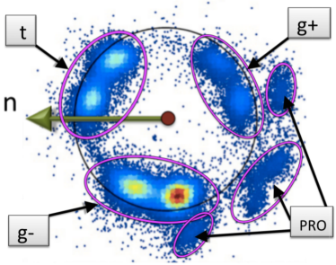
Figure 16: (Color online) Stereographic projection of level-$\gamma$ rotamers in the frame of figure 15 b) in combination with (14).

we have stereographic projected figure 15 b), in combination with the map (14). In figures 17 we identify the rotamers according to

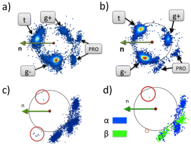
Figure 17: (Color online) The identification of rotamers and major secondary structures in figure 16. In a) the $\alpha$-helices, in b) the $\beta$-strands. In c) all prolines, and in d) prolines divided according to their $\alpha$-helical (blue) and $\beta$-stranded (green) assignment in PDB. Some apparent outliers have been high-lighted with red circles.

the $\alpha$-helical and $\beta$-stranded regions, and the rotamers for prolines.

The $\alpha$-helical rotamer distribution in figure 17 a) and $\beta$-stranded distribution in figure 17 b) have essentially the same latitude angle. But there is a visible difference in the longitudes. Each has a trimodal structure, and we again denote the rotamers as g$\pm$ and t. The distributions are related to each other by 120^o longitudinal rotations. It is noteworthy how the prolines shown in figures 17 c) and d) also reflect the backbone secondary structure, as assigned by PDB. In these figures we have also highlighted some apparent outlying prolines. These are located in two clusters.

There are also outliers that are outside of the range of the stereographic projection in figures 17. The projection - to the extent it has been plotted - covers a disk-like region around the north-pole i.e. around the tip of vector $\mathbf{t}$ in the figure. The far-away outliers can be visualized by properly rotating the sphere. The rotated sphere is shown in figure 18.

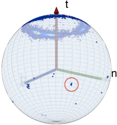
Figure 18: (Color online) An example of a group of five far away outliers in figure 15 b), made visible by rotating the sphere and highlighting with red circle. They all correspond to the same protein but with different PDB codes: 1FN8, 1FY4, 1FY5, 1GDN and 1GDQ. In each case, the outlier is in the residue number 65 A. Note that there are also several other far away outliers.

A number of far-away outliers are now visible. As an example, we have encircled one group of outliers. It pertains to the mutually related PDB entries 1FN8, 1FY4, 1FY5, 1GDN and 1GDQ. These outliers all have the same residue number 65 in the PDB data. It is a multiple position entry and the figure shows that one of these (A) is atypical.

Finally, as a concrete example of an amino acid we consider threonine, where the level-$\gamma$ consists of a C_γ and O_γ pair. In figure 19 a)

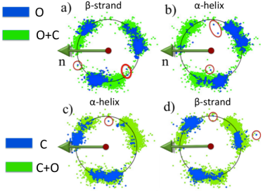
Figure 19: (Color online) a) O_γ (dark blue) in THR, with backbone in the $\beta$-stranded position. b) O_γ (dark blue) in THR, with backbone in the $\alpha$-helix position. c) Same as a) but for C_γ. d) Same as b) but for C_γ. Some apparent outliers are encircled. The (light green) background in each Figure consists of all O_γ and C_γ in THR.

we display (in blue) those O_γ atoms where the backbone is in a $\beta$-strand position according to PDB. In 19 b) we have (in blue) those O_γ where the backbone is in an $\alpha$-helix position. In figures 19 c) and d) we have the corresponding distributions for C_γ. The (green) background is made of all O_γ and C_γ atoms in our data set. Both the trimodal rotamer structure and its secondary structure dependence are clearly visible, both in O_γ and in C_γ. For the latter, the distribution matches that displayed in Figures 17 a) and b). Some apparent outliers have also been highlighted in Figures 19 by encircling them (with red).

I.6 Level-$\delta$ rotamers

I.6.1 Standard dihedral angle:

We proceed upwards along the side-chain, to describe level-$\delta$ atoms. We start with a coordinate frame which is centered at the C_γ atom. We note that in the case of ILE, two alternatives exist and we choose the C_γ carbon which is covalently bonded to the C_δ atom.

We set

$$\mathbf{t}_{\mathcal{X}2}=\frac{\mathbf{r}_{\gamma}-\mathbf{r}_{\beta}}{|\,\mathbf{r}_{\gamma}-\mathbf{r}_{\beta}\,|}$$

and we choose

$$\mathbf{n}_{\mathcal{X}2}=\frac{\mathbf{t}_{\mathcal{X}2}\times\mathbf{t}_{\mathcal{X}1}}{|\,t_{\mathcal{X}2}\times\mathbf{t}_{\mathcal{X}1}\,|}$$

The third vector $\mathbf{b}_{\mathcal{X}2}$ that completes the right-handed orthonormal triplet is given by

$$\mathbf{b}_{\mathcal{X}2}=\mathbf{t}_{\mathcal{X}2}\times\mathbf{n}_{\mathcal{X}2}$$

In figure 20

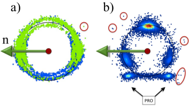
Figure 20: (Color online) a) Distribution of aromatic and b) non-aromatic level-$\delta$ C atoms, in the stereographic projection of the unit two-sphere centered at the C$\gamma$ atom. In a) the (dark) blue is C$\delta 1$ and (light) green is C$\delta 2$. Some outliers have been encircled, as examples. The (black) circles around the center denote the average distance of the distribution.

we show the distribution of heavy atoms in level-$\delta$, after stereographic projection (6). The longitude in these figures coincides with the standard $\mathcal{X}_{2}$ dihedral angle, modulo a global $\pi/2$ rotation around the center. In addition, we introduce the following version of (7)

$$f(\theta)=\frac{1}{1+\theta^{4}}$$ (18)

In the figure 20, we have separately displayed the distribution of the aromatic (a) and the non-aromatic (b) amino acids; we find that starting at level-$\delta$ this is a convenient bisection. A clear trimodal rotamer structure is present in figure 20 b). Some outliers have been highlighted with circles, as generic examples. In figure 21 a)

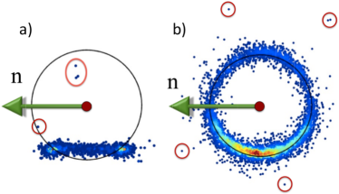
Figure 21: (Color online) a) The proline contribution to the non-aromatic level-$\delta$ atoms in Figure 20 b). Three apparent outliers have been encircled. b) The level-$\delta$ distribution of O atoms. The (black) circle denotes the average distance of the distribution from the center. Some outliers have been highlighters with red circles.

we have the proline contribution to figure 20 b) and in figure 21 b) we show the distribution of the O atoms at level-$\delta$. The latitude angles in O are highly restrained while the longitudinal angles are quite flexible. Some apparent outliers have been encircled in both figures 21, as generic examples.

Finally, as in figure 13 in figures 20 and 21 there is no visible sign of secondary structure: The standard ${\mathcal{X}}_{2}$ dihedral is backbone independent.

However, as in figures 14, in the backbone Frenet frames where the C_α is located at the center of the sphere, the secondary structure dependence becomes visible in the level-$\delta$ rotamers. As an example, we show in figure 22

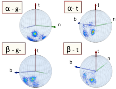
Figure 22: (Color online) Four figures that show the level-$\delta$ Frenet frame distributions corresponding to the level-$\gamma$ distributions in figures 14. The labeling is as follows: $\alpha$ - $g$- stand for $\alpha$-helical backbone secondary structure in $g$- rotamer in figures 14, $\alpha$ - $t$ stand for $\alpha$-helical backbone secondary structure in $t$ rotamer in figures 14, $\beta$ - $g$- stand for $\beta$-stranded backbone secondary structure in $g$- rotamer in figures 14 and $\beta$ - $t$ stand for $\beta$-stranded backbone secondary structure in $t$ rotamer in figures 14.

how some of the regions in figure 14 are seen on the surface of the ensuing C_α centered sphere, by the roller coasting observer. The examples we have displayed are the overlap of the $\alpha$-helical structures with the $g-$ rotamer (marked $\alpha$-$g-$ in the figure ) and $t$ rotamer ($\alpha$-$t$), and the overlap of the $\beta$-stranded structures with the $g-$ rotamer ($\beta$-$g-$) and $t$ rotamer ($\beta$-$t$). A secondary structure dependent trimodal rotamer structure is clearly present, in each of the distributions.

I.6.2 Secondary structure dependent level-$\delta$ rotamer angles:

Following (15)-(17) and figures 15-17 we proceed to visually inspect secondary structure dependence in the level-$\delta$ rotamers. For this, we define an orthonormal frame as follows:

$${\mathbf{t}}_{\gamma}\ =\ \frac{\mathbf{r}_{\gamma}-\mathbf{r}_{\beta}}{|\,\mathbf{r}_{\gamma}-\mathbf{r}_{\beta}\,|}$$

$$\mathbf{n}_{\gamma}\ =\ \frac{\mathbf{t}_{\gamma}\times\mathbf{t}_{\alpha}}{|\,\mathbf{t}_{\gamma}\times\mathbf{t}_{\alpha}\,|}$$

Finally,

$$\mathbf{b}_{\gamma}=\mathbf{t}_{\gamma}\times\mathbf{n}_{\gamma}$$

We start with the non-aromatic amino acids. In figure 23

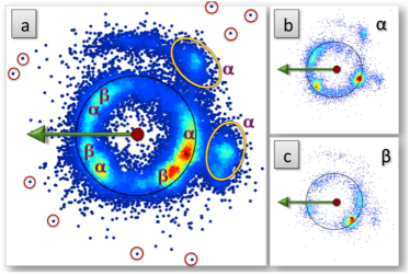
Figure 23: (Color online) The level-$\delta$ distribution of non-aromatic C atoms, in the stereographic projection. In figure a) we show the entire background, and in b) and c) those that have been classified as $\alpha$-helical and $\beta$-stranded, respectively. Some outliers have also been marked.

we show the distribution of all the C_δ non-aromatic atoms in our data set. In this figure we have also identified those apparent rotamers that are classified either as $\alpha$-helical or $\beta$-stranded in PDB. The figure shows that there is a clear secondary structure dependence in these rotamers. In figure 24

Figure 24: (Color online) The level-$\delta$ distribution of non-aromatic C atoms, in the stereographic projection and divided according to the level-$\gamma$ rotamers. In figure a) we show the $g$- rotamer, in figure b) we show the $t$ rotamer, in figure c) we have the $g$+ rotamer and in figure d) we show the $cis$-proline. The radii of the (black) circles coincide with the average latitude in figure 23 a). Some outliers have also been encircled.

we display the three level-$\gamma$ subsets of 23 a). Again, there is a clear secondary structure dependence in the rotamers. We have also encircled some apparent outliers in both figures 23 and 24. Far-away outliers also exist (not shown), these can be located and visualized by rotating the original sphere as in figure 18.

We proceed to the aromatic amino acids. In figure 25 a)

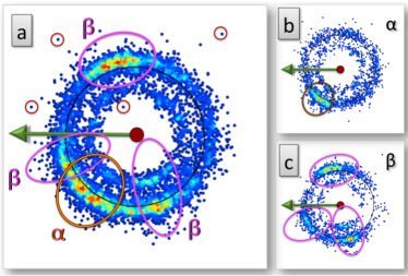
Figure 25: (Color online) Level-$\delta$ distribution of aromatic CD1 atoms PHE, TYR and TRP in the stereographic projection. In a) all CD1 atoms in our data set, and in b) and c) the $\alpha$-helical and $\beta$-stranded subsets, with rotamer states encircled . Some outliers have also been encircled in a).

we show all level-$\delta$ carbons (CD1 in PDB), these are PHE, TYR, TRP. In figures 25 b) and c) we show the subsets of 25 a) that have been classified as $\alpha$-helical resp. $\beta$-stranded in PDB. In 26 a)

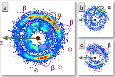
Figure 26: (Color online) Same as figure 25, but for the CD2 carbons according to PDB classification, including PHE, TYR, TRP and HIS. Some outliers have also been encircled in figure 26 a).

we show all level-$\delta$ carbons (CD2 in PDB) i.e. PHE, TYR, TRP and HIS. In figures 26 b) and c) we show the subsets of 26 a) that have been classified as $\alpha$-helical resp. $\beta$-stranded in PDB. In both figures 25 and 26 the secondary structure dependence is again manifest. In particular, both $\alpha$-helices and $\beta$-strands form clear rotamers. We have also highlighted some outliers, by encircling them.

I.7 Level$-\epsilon$ atoms

We proceed to the level-$\epsilon$ atoms. We follow the previous construction: We introduce a coordinate frame which is based at the C_δ carbon i.e. describes the point-of-view of an imaginary minuscule observer who has climbed up to C_δ along the side chain. We map the level-$\epsilon$ atoms on the surface of the two-sphere which is centered at the C_δ, followed by the stereographic projection.

Note that in the case of PHE and TYR two essentially identical choices can be made. In the case of TRP there are also two choices, and we choose the one denoted CD2 in PDB, it is covalently bonded to the higher level C atoms. In the case of HIS a framing could also be based on the level-$\delta$ N atom, but here we select the level-$\delta$ C atoms that are denoted CD2 in PDB.

The orthonormal triplet is now defined as follows,

$${\mathbf{t}}_{\delta}\ =\ \frac{\mathbf{r}_{\delta}-\mathbf{r}_{\gamma}}{|\,\mathbf{r}_{\delta}-\mathbf{r}_{\gamma}\,|}$$

$$\mathbf{n}_{\delta}\ =\ \frac{\mathbf{t}_{\delta}\times\mathbf{t}_{\alpha}}{|\,\mathbf{t}_{\delta}\times\mathbf{t}_{\alpha}\,|}$$

and

$$\mathbf{b}_{\delta}=\mathbf{t}_{\delta}\times\mathbf{n}_{\delta}$$

In figures 27 a)-f)

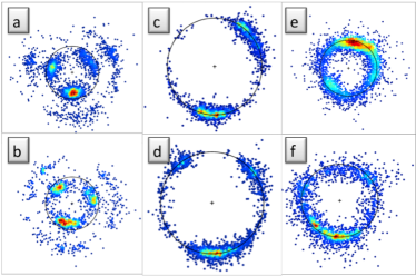
Figure 27: (Color online) Examples of rotamers in level-$\epsilon$ atoms; the black circles have the same radius in a) and b), in c) and d), and in e) and f). In figure a) the $\alpha$-helix and in b) the $\beta$-strand rotamers for for CE in MET and LYS; the structures outside the circle are LYS, those inside are MET. In figure c) the $\alpha$-helix and in d) the $\beta$-strand rotamers for for CE1 in PHE and TYR. In figure e) the $\alpha$-helix rotamers for OE1 in GLU and GLN, and in f) the $\alpha$-helix rotamers for OE2 in GLU (there is no GLN).

we show various examples of level-$\epsilon$ atoms. We observe that in addition of rotamers in the longitude, there are also rotamer-like variations in the latitude angle, as shown in black circles in each figure.

I.8 Level-$\zeta$ atoms

We continue to level-$\zeta$. We introduce the C_ϵ centered two-sphere with orthonormal triplet given by

$${\mathbf{t}}_{\epsilon}\ =\ \frac{\mathbf{r}_{\epsilon}-\mathbf{r}_{\delta}}{|\,\mathbf{r}_{\epsilon}-\mathbf{r}_{\delta}\,|}$$

$$\mathbf{n}_{\epsilon}\ =\ \frac{\mathbf{t}_{\epsilon}\times\mathbf{t}_{\alpha}}{|\,\mathbf{t}_{\epsilon}\times\mathbf{t}_{\alpha}\,|}$$

$$\mathbf{b}_{\epsilon}=\mathbf{t}_{\epsilon}\times\mathbf{n}_{\epsilon}$$

As an example, in figures 28

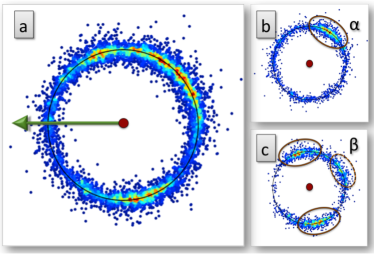
Figure 28: (Color online) Example of level-$\zeta$ rotamers. In figure a) we have all the C_ζ carbons in PHE and TYR. In figures b) and c) we show the subsets that correspond to $\alpha$-helical and $\beta$-stranded secondary structures, respectively.

we show the C_ζ carbons for PHE and TYR using stereographic projection. The figure 28 a) shows all C_ζ atoms, and figures 28 b) and c) show the $\alpha$-helical and $\beta$-stranded subsets. In the case of $\alpha$-helical secondary structures we identify one rotamer. In the case of $\beta$-stranded structures we observe three rotamers. We observe that the $\beta$-stranded rotamers are not distributed evenly. The rotamers are not related to each other by (regular) $120^{\rm o}$ rotations.

I.9 Level-$\eta$ atoms

We continue the process to the level-$\eta$ which is the final level in proteins. We follow our construction to define the C_ζ centered coordinate system, with

$${\mathbf{t}}_{\zeta}\ =\ \frac{\mathbf{r}_{\zeta}-\mathbf{r}_{\epsilon}}{|\,\mathbf{r}_{\zeta}-\mathbf{r}_{\epsilon}\,|}$$

$$\mathbf{n}_{\zeta}\ =\ \frac{\mathbf{t}_{\zeta}\times\mathbf{t}_{\alpha}}{|\,\mathbf{t}_{\zeta}\times\mathbf{t}_{\alpha}\,|}$$

$$\mathbf{b}_{\zeta}=\mathbf{t}_{\zeta}\times\mathbf{n}_{\zeta}$$

As before, we also introduce the ensuing stereographic projection.

As an example, in figures 29

Figure 29: (Color online) Example of level-$\eta$ rotamers. In figure a) we have all the N$\eta 2$ atoms in ARG. There are two very close rotamer states, that have been encircled. Some outliers have also been encircled. In figures b)-d) we show the subsets that correspond to loops, $\beta$-stranded and $\alpha$-helical secondary structures, respectively. Comparison of the figures reveals that the two very close-by rotamers in a) correspond to loops and $\alpha$-helices.

we display the N${\eta}2$ distribution in ARG. Now there is a very strong two-fold localization of the distribution, shown in figure 29 a). In figures b)-d) we consider the subsets, consisting of PDB secondary structures that are classified as loops b), $\beta$-strands c) and $\alpha$-helices d). These identify the two rotamers in figure 29 a). Some of the outliers are encircled, as examples, in a).

II Discussion

We have utilized recent developments in modern 3D visualization techniques and advances in virtual reality to describe how to construct an entirely C_α geometry based visual library of the backbone and side chain atoms. Our construction is based on progress in visualization that has taken place since the inception of the Ramachandran map. In lieu of a torus, our approach engages the geometry of a sphere and as such it has a direct ”what-you-see-is-what-you-have” visual correspondence to the protein structure. In particular, we utilize the geometrically determined discrete Frenet frames of Hu-2011 . We propose the concept of an imaginary observer, chosen so that the discrete Frenet frames determine the orientation of the observer when she roller-coasts along the backbone and climbs up the side chains. She maps the directions of all the heavy atoms on the surface of a two-sphere that surrounds her, exactly as these atoms are seen in her local frame like stars in the sky.

Since the discrete Frenet frames can be unambiguously determined in terms of the C_α trace only, we can analyze both the backbone atoms and the side chain atoms on equal footing, in a single geometric framework. This is not possible in the conventional Ramachandran approach, that assumes a priori knowledge of the peptide planes, to define the dihedral angles.

As examples of the approach, we have analyzed the orientation of various heavy atoms that are located both along the backbone and in the side chains. Our approach also enables a direct, visual identification of outliers.

In particular, we have found that in terms of the discrete Frenet frames, the secondary structure dependence becomes clearly visible in the rotamer structure, both in the case of the backbone atoms and in the case of the side chain atoms. Apparently this is not always the case, in conventional approaches such as Holm-1991 ; Rotkiewicz-2008 ; Li-2009 ; according to Dunbrack-2002 conventional secondary structure dependent rotamer libraries do not provide much more information than backbone-independent rotamer libraries. But by using the Frenet frame coordinate system chosen here, there is a clear correlation between secondary structures and rotamer positions. Thus the approach we have presented, can form a basis for the future development of a novel approach to the C_α trace problem. Unlike the existing approaches Holm-1991 ; Rotkiewicz-2008 ; Li-2009 the one we envision accounts for the secondary structure dependence in the heavy atom positions that we have revealed, which should lead to an improved accuracy in determining the heavy atom positions.

Acknowledgements

A.J. Niemi thanks A. Elofsson, J. Lee and A. Liwo for a discussion. This research hs been supported by a CNRS PEPS Grant, Region Centre Recherche d^′Initiative Academique grant, Cai Yuanpei Exchange Program, Qian Ren Grant at BIT, Carl Trygger’s Stiftelse för vetenskaplig forskning, and Vetenskapsrådet.

References

- (1)
- (2) V.B. Chen, W.B. Arendall III, J.J. Headd, D.A. Keedy, R.M. Immormino, G.J. Kapral, L.W. Murray, J.S. Richardson, D.C. Richardson, Acta Cryst. D66, 12 (2010)
- (3) R.A. Laskowski, M.W. MacArthur, D.S. Moss, J.M. Thornton, J. App. Cryst. 26 283 (1993)
- (4) X. Qu, R. Swanson, R. Day, J. Tsai, Curr. Protein Pept. Sci. 10 270 (2009)
- (5) P.L. Freddolino, C.B. Harrison, Y. Liu, Y. Schulten, Nature Phys. 6 751 (2010)
- (6) G.N. Ramachandran, C. Ramakrishnan, V. Sasisekharan, J. Mol. Biol. 7 95 (1963)
- (7) O. Carugo, K. Djinovic Carugo, Acta Cryst. D69, 1333 (2013)
- (8) J. Janin, S. Wodak, M. Levitt, B. Maigret, J. Mol. Biol. 125 357 (1978)
- (9) P.D. Adams, P.V. Afonine, G. Bunkóczi, V.B. Chen, I.W. Davis, N. Echols, J.J. Headd, L.-W. Hung, G.J. Kapral, R.W. Grosse-Kunstleve, A.J. McCoy, N.W. Moriarty, R. Oeffner, R.J. Read, D.C. Richardson, J.S. Richardson, T.C. Terwilliger, P.H. Zwart, Acta Cryst. D66 213 (2010)
- (10) G.N. Murshudov, A.A. Vagin, E.J. Dodson, Acta Cryst. D53 240 (1997)
- (11) R.A. Engh, R. Huber, Acta Cryst. A47 392 (1991)
- (12) R.A. Engh, R. Huber, in International Tables for Crystallography, Vol. F, pages 382–392; edited by M. G. Rossmann and E. Arnold (Kluwer Academic Publishers, Dordrecht, 2001)
- (13) J.W. Ponder, F.M. Richards, J. Mol. Biol. 193 775 (1987)
- (14) R.L. Dunbrack Jr., Curr. Op. Struc. Biol. 12 431 (2002)
- (15) H.M. Berman, J. Westbrook, Z. Feng, G. Gilliland, T.N. Bhat, H. Weissig, I.N. Shindyalov, P.E. Bourne, Nucl. Acids Res. 28 235 (2000)
- (16) S.C. Lovell, J. Word, J.S. Richardson, D.C. Richardson, Proteins 40 389 (2000)
- (17) R. Chandrasekaran, G.N. Ramachandran, Int. J. Protein Res. 2 223 (1970)
- (18) H. Schrauber, F. Eisenhaber, P. Argos, J. Mol. Biol. 230 592 (1993)
- (19) R.L. Dunbrack Jr., M. Karplus, J. Mol. Biol. 230 543 (1993)
- (20) M.S. Shapovalov, R.L. Dunbrack Jr., Structure 19 844 (2011)
- (21) T.A. Jones, J.-Y. Zou, S.W. Cowan, M. Kjeldgaard, Acta Cryst. A47 110 (1991)
- (22) I. Sillitoe, A.L. Cuff, B.H. Dessailly, N.L. Dawson, N. Furnham. D. Lee, J.G. Lees, T.E. Lewis, R.A. Studer, R. Rentzsch, C. Yeats, J.M. Thornton, C.A. Orengo, Nucleic Acids Res. 41(D1), D490 (2013)
- (23) A.G. Murzin, S.E. Brenner, T. Hubbard, C. Chothia, J. Mol. Biol. 247 536 (1995)
- (24) A. Roy, A. Kucukural, Y. Zhang, Nature Protocols 5 725 (2010)
- (25) T. Schwede, J. Kopp, N. Guex, M.C. Peitsch, Nucleic Acids Res., 31 3389 (2003)
- (26) Y. Zhang, Curr. Opin. Struct. Biol. 19 145 (2009)
- (27) K. Dill, S.B. Ozkan, T.R. Weikl, J.D. Chodera, V.A. Voelz, Curr. Op. Struct. Biol. 17 342 (2007)
- (28) H.A. Scheraga, M. Khalili, A. Liwo, Ann. Rev. Phys. Chem. 58 57 (2007)
- (29) L. Holm, C. Sander, Journ. Mol. Biol. 218 183 (1991)
- (30) M.A. DePristo, P.I.W. de Bakker, R.P. Shetty, T.L. Blundell, Prot. Sci. 12 2032 (2003)
- (31) S.C. Lovell, I.W. Davis, W.B. Arendall III, P.I.W. de Bakker, J.M. Word, M.G. Prisant, J.S. Richardson, D.C. Richardson, Proteins 50 437 (2003)
- (32) P. Rotkiewicz, J. Skolnick, Journ. Comp. Chem. 29 1460 (2008)
- (33) Y. Li, Y. Zhang, Proteins 76 665 (2009)
- (34) E.O. Purisima, H.A. Scheraga, Biopolymers 23 1207 (1984)
- (35) S. Hu, M. Lundgren, A.J. Niemi, Phys. Rev. E83 061908 (2011)
- (36) M. Lundgren, A.J. Niemi, F. Sha, Phys. Rev. E85 061909 (2012)
- (37) M. Lundgren, A.J. Niemi, Phys. Rev. E85 021904 (2012)
- (38) L. Schäfer, M. Cao, Journ. Mol. Struct. 333 201 (1995)
- (39) X. Jiang, C.-H. Yua, M. Cao, S.Q. Newton, E.F. Paulus, L. Schäfer, Journ. Mol. Struct. 403 83 (1997)
- (40) D.S. Berkholz, M.V. Shapovalov, R.L. Dunbrack Jr., P.A. Karplus, Structure 17 1316 (2009)
- (41) W.G. Touw, G. Vriend, Acta Cryst. D66 1341 (2010)