Liquid-state polaron theory of the hydrated electron revisited

Abstract

The quantum path integral/classical liquid-state theory of Chandler and co-workers, created to describe an excess electron in solvent, is re-examined for the hydrated electron. The portion that models electron-water density correlations is replaced by two equations: the range optimized random phase approximation (RO-RPA), and the DRL approximation to the “two-chain” equation, both shown previously to describe accurately the static structure and thermodynamics of strongly charged polyelectrolyte solutions. The static equilibrium properties of the hydrated electron are analyzed using five different electron-water pseudopotentials. The theory is then compared with data from mixed quantum/classical Monte Carlo and molecular dynamics simulations using these same pseudopotentials. It is found that the predictions of the RO-RPA and DRL-based polaron theories are similar and improve upon previous theory, with values for almost all properties analyzed in reasonable quantitative agreement with the available simulation data. Also, it is found using the Larsen, Glover and Schwartz pseudopotential that the theories give values for the solvation free energy that are at least three times larger than that from experiment.

I Introduction

The solvated electron, the smallest anion, is a highly reactive species, with a lifetime $\sim 10^{-3}$ seconds in pure water at room temperature.Mozumder (1999) It is an intermediate in many water-based chemical reactions.Buxton et al. (1988)

A large part of our understanding of the hydrated electron has come from theory and simulation.Feng and Kevan (1980); Sprik et al. (1986); Schnitker and Rossky (1987a); Barnett et al. (1988); Turi and Borgis (2002); Jacobson and Herbert (2010); Laria et al. (1991); Turi and Rossky (2012) Most of the modern efforts have modeled the electron-water and water-water interactions through pseudopotentials. Results of this approach and others have led to a view that the hydrated electron is a localized, self-trapped object. Recently, however, this view has been challenged,Larsen et al. (2010) and the subject is currently controversial.Turi and Madarasz (2011); Jacobson and Herbert (2011); Larsen et al. (2011); Herbert and Jacobson (2011); Turi and Rossky (2012); Uhlig et al. (2012); Casey et al. (2013)

Our primary interest here though is with simpler theoretical approaches, the aim being ultimately to go beyond the basic system of a single electron in infinite water, to study bipolarons for example.Laria et al. (1991) The question then is whether, given a particular pseudopotential, the theory can give accurate results in comparison with more complex methods such as mixed quantum/classical molecular dynamics simulation.

One successful theory to date has been the RISM-polaron one of Chandler and co-workers.Chandler et al. (1984); Nichols et al. (1984); Laria et al. (1991) In their work on the hydrated electron, Laria, Wu and Chandler (LWC) found that the theory gave reasonable predictions in comparison with simulation for quantities such as the excess chemical potential and electron polymer size. However, its modeling of electron-water density correlations was not as good as one would expect, local structure usually being a strong point of liquid-state theory.Hansen and McDonald (1986); Schweizer and Curro (1997); Curro et al. (1999); Heine et al. (2005) LWC concluded that the equation developed by them for the electron-water radial distribution function was the primary cause. Also, in some cases, the theory predicted a “super-trapped” electron polymer, but there has been no subsequent supporting evidence for its existence.

Since the work of LWC, two liquid-state theories, the range optimized random phase approximation (RO-RPA)Donley et al. (2004) and the approximation of Donley, Rajasekaran and Liu (DRL)Donley et al. (1998) to the “two-chain” equation, have been developed. Both theories have been shown to give quantitatively accurate descriptions of the structure and thermodynamics of strongly charged polyelectrolyte solutions.Donley et al. (2004); Donley and Heine (2006) In particular, it was found that site-level correlations included in these theories, but not captured well by the LWC liquid-state element, were important.

One purpose of the present work then is to revisit the RISM-polaron theory of the hydrated electron, but instead use the RO-RPA and DRL equations for the electron-water radial distribution functions. Employing a few pseudopotentials should be sufficient to determine the accuracy of the theory and which elements need improvement. However, there are important qualitative differences among the candidate pseudopotentials. So using theory to explore other phenomena is suspect until this controversy is settled. A second purpose then is to compare with as many pseudopotentials involved in the current discussion as possible. As will be shown below, the theory can shed light on some questions that have not been convincingly answered as yet.

The remainder of this paper is organized as follows. In Sec. II the basic elements of the RISM-polaron theory, and then the RO-RPA and DRL theories, are described briefly. In Sec. III various other ingredients needed by the theory are discussed, including the five pseudopotentials used in the analysis. In Sec. IV the numerical procedure to solve the theory is described, and in Sec. V results are presented. Finally in Sec. VI the work is summarized and directions for further work are discussed.

II Theory

II.1 Review of RISM-polaron theory

In this section, the RISM-polaron theory of Chandler and co-workers Chandler et al. (1984); Nichols et al. (1984); Laria et al. (1991) is reviewed briefly, with the main approximations of the theory highlighted. The notation is the same as for LWC where relevant, except in a few instances.

An important thermodynamic quantity for a solvated electron is the solvation free energy or excess chemical potential, $\Delta\mu$, which is the work needed to add a free electron to the solvent. In terms of the electron-solvent equilibrium free energy, $F$,

$$\Delta\mu=F-F_{free},$$ (II.1)

where $F_{free}$ is the free energy of the electron and solvent system when the electron is free and far away. In the canonical ensemble,

$$\beta F=-{\rm ln}\ Z,$$ (II.2)

where $\beta$ is the inverse of $k_{B}T$ with $k_{B}$ being Boltzmann’s constant and $T$ the absolute temperature. The partition function is

$$Z={\rm Tr}[\rho_{S}],$$ (II.3)

with the statistical density matrix element:

$$\rho_{S}({\bf x},\{{\bf R}\};{\bf x}^{\prime},\{{\bf R}^{\prime}\})=\langle{\bf x},\{{\bf R}\}|e^{-\beta H}|{\bf x}^{\prime},\{{\bf R}^{\prime}\}\rangle.$$ (II.4)

Here, ${\bf x}$ is the electron position and $\{{\bf R}\}$ is the set of solvent coordinates, with ${\bf R}_{is}$ (denoted as ${\bf r}_{i}^{(s)}$ in LWC) being the position of site $s$ on solvent molecule $i$. Also, $H$ is the full electron and solvent Hamiltonian, and $|{\bf x},\{{\bf R}\}\rangle$ is an eigenket in the position basis of the electron-solvent system.

It is convenient to evaluate $\rho_{S}$ using path integrals. An especially appealing method is to integrate out the degrees of freedom of the surrounding medium, leaving one that depends only on the electron position ${\bf x}$.Feynman and Hibbs (2010)

Experiments involving electrons in water typically occur near room temperature. At $T$=298 K, the electron thermal wavelength $\lambda_{e}=\sqrt{{\beta\hbar^{2}\over m}}\simeq 17.2$Å, which is large. Here, $\hbar$ is Planck’s constant divided by $2\pi$ and $m$ is the electron mass. Thus, quantum effects must be considered in determining its properties. On the other hand, the thermal wavelength for water is around $0.1$Å, which is much smaller than the size of water and the range of the internal forces of the liquid. It seems reasonable then to treat the properties of water using classical methods.

Treating the solvent classically enormously simplifies the integration over their degrees of freedom. Chandler, Singh and Richardson (CSR) find, to second order in the electron-solvent interactions, that the effective diagonal statistical density matrix element for the electron is:Chandler et al. (1984)

$$\rho_{S}({\bf x},{\bf x})= \ C_{1}\int{\cal D}\{{\bf R}\}\rho_{S}({\bf x},\{{\bf R}\};{\bf x},\{{\bf R}\})$$

$$\simeq \ C_{2}\int_{\bf x}^{\bf x}{\cal D}[{\bf r}(\tau)]exp(S[{\bf r}(\tau)]),$$ (II.5)

where $\int{\cal D}\{{\bf R}\}$ denotes an integral over the space of solvent positions $\{{\bf R}\}$, $C_{1}$ and $C_{2}$ are constants, and $\int_{\bf x}^{\bf x}{\cal D}[{\bf r}(\tau)]$ denotes an integral over all electron paths ${\bf r}(\tau)$ in imaginary time $\tau$, $0\leq\tau\leq\beta\hbar$ that start and end at position ${\bf x}$. The imaginary time action is

$$S=S_{0}+S_{I}$$ (II.6)

where the electron kinetic energy term is

$$S_{0}[{\bf r}(\tau)]=-{m\over 2\hbar}\int_{0}^{\beta\hbar}d\tau\bigl{|}{\dot{\bf r}(\tau)}\bigr{|}^{2},$$ (II.7)

the dot denoting a time derivative, and the solvent-mediated electron-electron interaction term is

$$S_{I} [{\bf r}(\tau)]=-\rho\sum_{s}\beta{\hat{u}}_{es}(0)-$$ (II.8)

$$\ {1\over 2(\beta\hbar)^{2}}\int_{0}^{\beta\hbar}d\tau\int_{0}^{\beta\hbar}d\tau^{\prime}v(|{\bf r}(\tau)-{\bf r}(\tau^{\prime})|).$$

Here, $\rho=N/V$ is the average solvent molecular number density with $N$ being the number of solvent molecules in the liquid volume $V$. The term ${\hat{u}}_{es}(0)$ is the zero wavevector value of the Fourier transform of $u_{es}(r)$, which is the (pseudo-)potential between the electron and a site $s$ on the solvent molecule. For the water pseudopotentials used in this work, the index $s$ takes three values corresponding to the oxygen and two hydrogen atoms.

The medium-induced potential has the familiar RPA form:

$$v(r)=-\beta^{2}\sum_{s,s^{\prime}}u_{es}*\chi_{ss^{\prime}}*u_{s^{\prime}e}(r),$$ (II.9)

where the asterisks (*) denote convolutions and $r=|{\bf r}|$. Also, $\chi_{ss^{\prime}}(r)$ is the density-density correlation function between solvent sites $s$ and $s^{\prime}$:

$$\chi_{ss^{\prime}}(r)=\bigl{\langle}({\hat{\rho}}_{s}({\bf r})-\rho)({\hat{\rho}}_{s^{\prime}}(0)-\rho)\bigr{\rangle},$$ (II.10)

where the brackets denote an ensemble average, and the microscopic density of solvent site $s$ is

$${\hat{\rho}}_{s}({\bf r})=\sum_{i=1}^{N}\delta({\bf r}-{\bf R}_{is}),$$ (II.11)

with $\delta({\bf r})$ being the Dirac “delta” function at position ${\bf r}$.

The RPA, as a generalization of Debye-Hückel theory, is strictly valid only for weak interactions, which would appear not to be the case for the solvated electron. As such, CSR give arguments for extending the validity of Eq.(II.9) to much stronger interactions by optimizing $S_{I}$ through the substitution of the bare potential $-\beta u_{es}(r)$ with the direct correlation function $c_{es}(r)$, defined by the RISM equation.Chandler and Andersen (1972) For this system, the RISM equation is

$$\rho h_{es}(r)=\sum_{s^{\prime}}\omega_{e}*c_{es^{\prime}}*\chi_{s^{\prime}s}(r),$$ (II.12)

where $h_{es}(r)=g_{es}(r)-1$, with the electron-solvent radial distribution function,

$$g_{es}(r)={1\over\beta\hbar}\int_{0}^{\beta\hbar}d\tau\ {1\over N}\sum_{i=1}^{N}\langle V\delta({\bf r}-{\bf r}(\tau)+{\bf R}_{is})\rangle,$$ (II.13)

where the brackets denote a thermal average over the configurations of the electron and solvent. Note that this is a site-site function, rather than being defined relative to the electron center-of-mass.

The function $\omega_{e}(r)$ in Eq.(II.12) describes site-site electron self-correlations. It is defined as

$$\omega_{e}(r)={1\over\beta\hbar}\int_{0}^{\beta\hbar}d\tau\ \omega_{e}(r,\tau),$$ (II.14)

where

$$\omega_{e}({\bf r},\tau-\tau^{\prime})=\langle\delta({\bf r}-{\bf r}(\tau)+{\bf r}(\tau^{\prime}))\rangle,$$ (II.15)

the brackets denoting an average over all paths ${\bf r}(\tau)$ weighted by the imaginary time action given by Eq.(II.6) above.

In this manner,

$$v(r)\rightarrow-\sum_{ss^{\prime}}c_{es}*\chi_{ss^{\prime}}*c_{s^{\prime}e}(r).$$ (II.16)

For polymer molecules, this hypernetted-chain (HNC)Hansen and McDonald (1986) form for the medium-induced potential was derived by Melenkevitz, Schweizer and CurroMelenkevitz et al. (1993) using the density functional theory of Chandler, McCoy and Singer (CMS)Chandler et al. (1986). The substitution of $-\beta{\hat{u}}_{es}(0)$ in Eq.(II.8) with ${\hat{c}}_{es}(0)$ is an ansatz.

The approximate integrating out of the degrees of freedom of the solvent as done by CSR is unusual in that these degrees of freedom are considered “slow”Chandler et al. (1984) compared with the fluctuations of the electron. Instead, the fast degrees of freedom are usually integrated out, they then providing a smooth background force and thermal bath for the slower degrees of freedom of interest.Langer (1971) At the least, the degrees of freedom with similar relaxation timescales are integrated out, such as for polymer melts and solutions.Melenkevitz et al. (1993) For example, in many mixed quantum/classical Monte Carlo and molecular dynamics (MD) treatments of the hydrated electron, the electron motion is approximated as responding instantaneously to any change in the surrounding solvent.Barnett et al. (1988) This approximation is opposite to that done by CSR. So it can be expected for the hydrated electron that, by truncating the medium-induced potential at second order in the potential $u_{es}(r)$ as done above, some of the anisotropy of the electron-water correlations is sure to be lost.Laria et al. (1991) Though to what degree will be shown partly in the results to follow.

To compute the free energy and electron self-correlation function, the effective one-electron path integral, Eq.(II.5) can be evaluated by Monte Carlo simulation.Wu (1991); Sumi and Sekino (2004) However, a popular alternative is to define an effective interaction action,Feynman et al. (1962)

$$S_{ref}=-{1\over 2}\sum_{n\neq 0}\gamma_{n}|{\bf r}_{n}|^{2},$$ (II.17)

where the mode ${\bf r}_{n}$ is the Fourier transform of the electron imaginary time position ${\bf r}(\tau)$:

$${\bf r}_{n}={1\over\beta\hbar}\int_{0}^{\beta\hbar}d\tau\ {\bf r}(\tau)e^{i\Omega_{n}\tau},$$ (II.18)

with frequencies $\Omega_{n}=2\pi n/(\beta\hbar)$, and $\gamma_{n}$ is a mode dependent constant.

Then, the action $S=S_{0}+S_{ref}+\Delta S$, with $\Delta S=S_{I}-S_{ref}$. With $\Delta S=0$, the path integral can be solved exactly analytically. In this way, the free energy is expanded to first order in $\Delta S$ yielding an expression that can be minimized with respect to the coefficients $\gamma_{n}$ to obtain an upper bound on the true free energy. The resultant equation for the $\gamma_{n}$ is:Chandler et al. (1984)

$$\gamma_{n}= -{1\over 6\pi^{2}}\int_{0}^{\infty}dk\ k^{4}{\hat{v}}(k)\times$$ (II.19)

$${1\over\beta\hbar}\int_{0}^{\beta\hbar}d\tau\ {\hat{\omega}}_{e}(k,\tau)[1-\cos(\Omega_{n}\tau)],$$

where ${\hat{v}}(k)$ and ${\hat{\omega}}_{e}(k,\tau)$ are the Fourier transforms of the medium-induced potential Eq.(II.16), and time dependent electron self-correlation function Eq.(II.15), respectively. The latter function is computed self-consistently using the effective action $S_{0}+S_{ref}$. Note that the direct correlation function $c_{es}(r)$ also varies with changes in the electron self-correlations, yet terms due to that don’t appear in Eq.(II.19), even though they are large. The reason is that the variations of $c_{es}(r)$ in the two terms of $S_{I}$, Eq.(II.8) cancel. So, the ansatz of $-\beta{\hat{u}}_{es}(0)\rightarrow{\hat{c}}_{es}(0)$ is an important one.

Feynman’s path integral polaron formalism has been used in other areas at least since the work of Edwards on neutral polymers.Doi and Edwards (1986) He and others have found that for real polymers, reference actions such as Eq.(II.17) need to be used with care as they can give erroneous results. For example, des Cloizeaux showed that using Eq.(II.17), and evaluating its coefficients via the free energy minimization scheme above gave incorrect scaling for the size of a neutral polymer in solution.des Cloizeaux and Jannink (1991) The cause is thought to be the self-avoidance property of a real polymer. So, while this problem appears not to be an issue for the electron, this subtlety should be kept in mind.

Since $\omega_{e}(r)$ can be computed using the effective action $S_{0}+S_{ref}$, the theory is completed by specifying the electron-solvent potentials $u_{es}(r)$, radial distribution functions $g_{es}(r)$, and the solvent density-density correlation function $\chi_{ss^{\prime}}(r)$. The pseudopotentials used will be discussed in Sec. III.2 below. The method of obtaining $\chi_{ss^{\prime}}(r)$ is very similar to LWC, and will be discussed in Sec. III.1 below. Similar to LWC, expressions for $g_{es}(r)$ will be borrowed from classical liquid-state theory; however, the particular liquid-state theories used will differ. Those will be discussed in the next section.

Using the variational form for the free energy, and Eq.(II.1), an expression for $\Delta\mu$ can be obtained. It is given in LWC.Laria et al. (1991) Other useful properties of the solvated electron are its average kinetic energy, $\langle ke\rangle$, potential energy, $\langle pe\rangle$, and polymer diameter ${\cal R}(\beta\hbar/2)$. Expressions for all of these quantities are given in LWC,Laria et al. (1991) with $\langle ke\rangle$ also in Malescio and Parrinello.Malescio and Parrinello (1987) Another useful property is the electron polymer radius of gyration, the square of which is

$$R_{g}^{2}\equiv {1\over\beta\hbar}\int_{0}^{\beta\hbar}d\tau\ \langle({\bf r}(\tau)-{\bf r}_{cm})^{2}\rangle$$

$$= 6\sum_{n=1}^{\infty}{1\over m\beta\Omega_{n}^{2}+\gamma_{n}},$$ (II.20)

where the last expression was derived using the reference action $S_{0}+S_{ref}$ above. Here, ${\bf r}_{cm}$ is the position of the polymer center of mass. Predictions for all these properties will be given below.

II.2 Review of RO-RPA and DRL liquid-state theories

In this section, two theories that give predictions for the radial distribution function in molecular liquids are reviewed briefly. These will be used as self-consistent inputs to the hydrated electron theory through Eq.(II.12).

II.2.1 RO-RPA

In the RPA, the intermolecular correlation function $h_{es}(r)$ is represented by a simple expression in terms of the intermolecular potentials and pair intramolecular correlation functions. For the electron-solvent system it has the form:

$$\rho h_{es}(r)=-\sum_{s^{\prime}}\omega_{e}*\beta u_{es^{\prime}}*\chi_{s^{\prime}s}(r).$$ (II.21)

As can be seen, this equation is identical to the RISM equation, Eq.(II.12), with the substitution $-\beta u_{es}(r)\rightarrow c_{es}(r)$, the RISM equation itself reducing to the Ornstein-Zernike (OZ) equationHansen and McDonald (1986) for a liquid of atoms.

As discussed in Sec. II.1 above, the RPA is not expected to work well for systems with strong interactions such as that experienced by the hydrated electron. One sign of this breakdown is that for strong repulsive interactions, the radial distribution function will be negative at short distances, even though it strictly is a positive quantity.

In OZ theory, for atoms interacting with potentials that are hard-core for distances $r<\sigma$, and mildly attractive for $r>\sigma$, one solution to the problem is to employ the mean spherical approximation (MSA) closure.Hansen and McDonald (1986) This closure for a single component liquid consists of demanding that $g(r)$ be exactly zero for $r<\sigma$, and $c(r)=-\beta u(r)$ for $r>\sigma$, where $u(r)$ is the attractive potential. In this manner, one solves for $g(r)$ for $r>\sigma$ and $c(r)$ for $r<\sigma$. An analogous method, the Optimized-RPA (ORPA), can be used to optimize the RPA free energy.Andersen and Chandler (1971) The MSA closure has found much use in RISM and polymer RISM theory,Schweizer and Curro (1997) and has been shown to be diagrammatically proper for the polymer versionMelenkevitz and Curro (1997) of the theory of Chandler, Silbey and Ladanyi.Chandler et al. (1982)

The limitation to this approach though is that if particles interact with Coulomb forces, the long-ranged potential may itself produce strong repulsion. In this case, the OZ-MSA or ORPA method will still yield a $g(r)$ that is negative for distances outside the hard-core range $\sigma$.

A remedy is to notice that a strongly repulsive Coulomb interaction, as far as the radial distribution function is concerned, produces essentially the same effect as a hard-core potential, namely making $g(r)$ very close to zero at small (or not so small for polyelectrolytes) $r$.Donley et al. (2004) Given that, replace the potential $u(r)$ by an optimized one, ${\tilde{u}}(r)$, which has an effective hard-core range of $\sigma^{eff}$. The range is chosen to have the smallest value such that $g(r)$ is positive for all $r>\sigma^{eff}$, subject to the constraint that $\sigma^{eff}\geq\sigma$. As for the MSA, inside the effective hard-core, ${\tilde{u}}(r)$ is determined by enforcing the constraint $g(r)=0$, and outside, ${\tilde{u}}(r)$ equals $u(r)$. For the electron-solvent case, each potential $u_{es}(r)$ in Eq. (II.21) is replaced by an optimized one ${\tilde{u}}_{es}(r)$ with their own effective hard-core diameters $\sigma_{es}^{eff}$.

This RO-RPA theory has been shown to give predictions for the static structure factor and osmotic pressure of strongly charged polyelectrolyte solutions that are in quantitative agreement with simulation and experiment.Donley and Heine (2006)

II.2.2 DRL

Another successful approach toward understanding the structure of molecular liquids is to notice that, as an electron in solvent can be represented as a single electron in an effective field, so can the pair correlations between two molecules be represented as a configurational average of these two molecules in an effective field. Following this idea leads one to the two-chain equation for the radial distribution function. The equation was first suggested by Chandler and co-workers,Chandler et al. (1986); Laria et al. (1991) and later derived by Donley, Curro and McCoyDonley et al. (1994) using CMS density functional theory.

For electron-solvent correlations, the two-chain equation is

$$g_{es}(r)={1\over\beta\hbar}\int_{0}^{\beta\hbar}d\tau\Bigl{\langle} exp\bigl{[}-V_{eff}([{\bf r}(\tau^{\prime})],\{{\bf R}_{1}\})\bigr{]}\times$$ (II.22)

$$V\delta({\bf r}-{\bf r}(\tau)+{\bf R}_{1s})\Bigr{\rangle},$$

where the brackets denote a configurational average of the electron polymer and solvent molecule 1, $\{{\bf R}_{1}\}$ denotes the set of coordinates of that solvent molecule, and the effective electron-solvent interaction potential is

$$V_{eff}([{\bf r}(\tau^{\prime})],\{{\bf R}_{1}\})={1\over\beta\hbar}\int_{0}^{\beta\hbar}d\tau^{\prime}\ \sum_{s^{\prime}}v_{es^{\prime}}^{eff}({\bf r}(\tau^{\prime})-{\bf R}_{1s^{\prime}}).$$ (II.23)

Note the similarity of Eq.(II.22) with Eq.(II.13).

The effective pair electron-solvent interaction potential in Eq.(II.23) is

$$v_{es}^{eff}(r)=\beta u_{es}(r)+v_{es}(r),$$ (II.24)

where the electron-solvent medium-induced potential has an HNC form:

$$v_{es}(r)=-\sum_{tt^{\prime}}c_{et}*\chi_{tt^{\prime}}*c_{t^{\prime}s}(r),$$ (II.25)

with $c_{es}(r)$ and $\chi_{ss^{\prime}}(r)$ being defined by Eqs.(II.12) and (II.10), respectively. The solvent direct correlation function $c_{ss^{\prime}}(r)$ is defined by a RISM equation similar to Eq.(II.12).

For the solvated electron, LWC approximated Eq.(II.22) as

$$g_{es}(r)\approx exp\bigl{[}-\sum_{s^{\prime}}\omega_{e}*v_{es^{\prime}}^{eff}*\omega_{s^{\prime}s}(r)\bigr{]},$$ (II.26)

where the solvent intramolecular correlation function

$$\omega_{ss^{\prime}}(r)=\bigl{\langle}\delta({\bf r}-{\bf R}_{1s}+{\bf R}_{1s^{\prime}})\bigr{\rangle},$$ (II.27)

with the brackets denoting an ensemble average over the solvent.

While giving predictions for the hydrated electron size and chemical potential that were in reasonable agreement with simulation, LWC thought that the weakest element of their theory was Eq.(II.26). One reason is that molecular averaging over the effective pair potential, Eq.(II.24), cuts off the water Coulomb potential at the size of the molecule, water being charge neutral. In that manner angular correlations between the electron and the individual water atoms beyond the molecule size are lost, reducing the polarization effects of the water.Laria et al. (1991)

A further issue brought to light in the use of Eq.(II.26) for polyelectrolytes is that it exaggerates the repulsion between like charged molecules due to the neglect of site level correlations.Donley et al. (2005) We have investigated this effect for the hydrated electron by solving Eq.(II.22) by simulation using the “cloud” model. In this model, the electron polymer is replaced by a single site, but to retain some effects of the smearing of the electron charge, the electron-water potential is replaced by $\omega_{e}*u_{es}(r)$. It was found that the predictions for $g_{es}(r)$ were very close to those of Eq.(II.26) indicating that electron site-level correlations are important even for a compact electron polymer.

As such, it seems reasonable to include these site level correlations in some way. An approximation to the two-chain equation by Donley, Rajasekaran and Liu (DRL) does this.Donley et al. (1998); Donley (2002, 2004) For the electron-solvent system it is as follows.

Define a function $x_{es}(r,\lambda)$ for which the variable $\lambda$ is a measure of the strength of the effective interaction, Eq.(II.24). The function has $\lambda$ endpoints that are powers of the radial distribution function: $x_{es}(r,1)=g_{es}(r)^{\eta}$ and $x_{es}(r,0)=g_{es}^{ref}(r)^{\eta}$, where $g_{es}^{ref}(r)$ is for a reference system, which could be a hard-core one. The DRL equation then is:

$$x_{es}(r,\lambda)=x_{es}(r,0)-\eta\sum_{s^{\prime}}\omega_{e}*\Gamma_{es^{\prime}}(\lambda)*\omega_{s^{\prime}s}(r),$$ (II.28)

where

$$\Gamma_{es}(r,\lambda)=\delta v_{es}^{eff}(r)\int_{0}^{\lambda}d\lambda^{\prime}\ x_{es}(r,\lambda^{\prime}),$$ (II.29)

and

$$\delta v_{es}^{eff}(r)=v_{es}^{eff}(r)-v_{es}^{eff\_ref}(r).$$ (II.30)

The charging integral in $\Gamma_{es}(r,\lambda)$ is performed with the effective interaction $\delta v_{es}^{eff}(r)$ held constant. The term $v_{es}^{eff\_ref}(r)$ is the value of the effective potential for the reference system. The exponent $\eta=1/2$.

A further approximation is to assume that $x_{es}(r,\lambda)$ in $\Gamma_{es}(r,\lambda)$ varies with $\lambda$ as a simple power:Donley (2002)

$$x_{es}(r,\lambda)\approx x_{es}(r,0)^{1-\lambda}x_{es}(r,1)^{\lambda}.$$ (II.31)

This form allows the charging integral to be computed analytically. The accuracy of this approximation was determined by also solving the theory by computing the charging integral $\Gamma_{es}(r,\lambda)$ directly. This was done by discretizing $x_{es}(r,\lambda)$ in $\lambda$ and solving the resultant difference equations derived from Eqs.(II.28) and (II.29) above. It was found that the results for $\Delta\mu$ and $R_{g}$ differed by at most a few percent in the cases examined. As such, only results using Eq.(II.31) will be shown here.

Given the potentials $u_{es}(r)$, intramolecular structure functions $\omega_{ss^{\prime}}(r)$ and $\omega_{e}(r)$, and solvent correlations embodied in $\chi_{ss^{\prime}}(r)$ (and thus solvent direct correlations $c_{ss^{\prime}}(r)$), Eqs. (II.12), (II.24), (II.25), and (II.28)-(II.31) form a closed set that can be solved numerically. The procedure to do so will be described in Sec. IV below.

III Other ingredients

III.1 Water structure functions

As mentioned in Sec. II, the water density-density correlation function, $\chi_{ss^{\prime}}(r)$, is a necessary input to the theory. In LWC, an MD simulation of the single point charge (SPC) water model was used to determine the local structure of the water. Then the long wavelength behavior of $\chi_{ss^{\prime}}(r)$ was corrected.Laria et al. (1991)

The method here was very similar, but instead of the SPC model, the extended SPC (SPC/E) was used. The SPC/E model has been shown to give more realistic local correlations, pressure and dielectric constant than the SPC.van der Spoel et al. (1998); Wu et al. (2006)

The MD simulation was conducted using the LAMMPS package for classical systems.Plimpton (1995) Periodic boundary conditions, a particle-particle particle-mesh solver and a Nose-Hoover (constant NVT) thermostat were used. The water molecule bond lengths were held fixed using the SHAKE algorithm. Details of the SPC/E potentials are given elsewhere.van der Spoel et al. (1998) The simulation consisted of $2\times 10^{4}$ water molecules at a temperature of 298 K and density of $0.997\ {\rm g/cm^{3}}$. This gave a box length $L\simeq 84.347$Å. Integration of the equations of motion was done with a timestep of 2 fs and the simulation was run to 20 ns. The initial state was random and equilibrium was reached at most by 4 ns. The equilibrium correlations functions $g_{ss^{\prime}}(r)$, $s=O$ and $H$, were then computed using data for times greater than 4 ns.

The partial water structure functions $\chi_{ss^{\prime}}(r)$, Eq.(II.10), were computed using the standard relation:Hansen and McDonald (1986)

$$\chi_{ss^{\prime}}(r)=\rho\omega_{ss^{\prime}}(r)+\rho^{2}h_{ss^{\prime}}(r),$$ (III.1)

where $h_{ss^{\prime}}(r)=g_{ss^{\prime}}(r)-1$, and the intramolecular structure function, Eq.(II.27), was computed analytically in the SPC/E model.

It is important to the theory to model accurately the correlation functions at small wavevector.Laria et al. (1991) To increase this accuracy then, the Fourier transforms of the $\chi_{ss^{\prime}}(r)$, ${\hat{\chi}}_{ss^{\prime}}(k)$, were also computed directly for $k<1\ {\rm\AA}^{-1}$ using a set of wavevectors appropriate to the cubic simulation box. The Fourier transforms of the $h_{ss^{\prime}}(r)$ extracted from these ${\hat{\chi}}_{ss^{\prime}}(k)$ were then fit to a power series in $k^{2}$ up to $k^{6}$. The $k=0$ coefficient for all factors was set to the average value of the initial independent fits. This average gave a compressibility of $4.55\times 10^{-5}$ atm^-1, close to the experimental value of $4.58\times 10^{-5}$. The $k^{2}$ coefficients were then adjusted slightly to give a dielectric constant of $77$.Høye and Stell (1976); Chandler (1977) These series were then joined with the data for $k\geq 1\ {\rm\AA}^{-1}$ obtained via $g_{ss^{\prime}}(r)$ to give values for ${\hat{\chi}}_{ss^{\prime}}(k)$ for all $k$.

As discussed in the next section, one pseudopotential used, that of Larsen, Glover and Schwartz, has a third type of site, call it X, on the water molecule.Larsen et al. (2010) Bulk water correlations were thus also needed for it, and were obtained as follows. In the MD simulation done here, all averages were computed afterward using snapshots (taken at equally spaced times) of the simulation configuration. Since the relative position of site X was known it was then straightforward to add its coordinates for every molecule to the stored simulation configurations. The correlation functions $g_{ss^{\prime}}(r)$ and ${\hat{\chi}}_{ss^{\prime}}(k)$ with $s,s^{\prime}$ now including site X, were then computed in the same manner as above.

III.2 Pseudopotentials

The last ingredient of the theory is the choice of electron-solvent potential. Since the water is being treated classically, this potential must incorporate quantum effects, such as the orthogonality of the wavefunction of the solvated electron to those of the bound water electrons, in some manner.

There are currently a number of theories for the electron-water pseudopotential.Sprik et al. (1986); Schnitker and Rossky (1987b); Turi and Borgis (2002); Jacobson and Herbert (2010); Larsen et al. (2010) Five of these will be implemented here, all having been used or optimized within the SPC model of water.

The first two models, denoted in LWC as model I and II, were used by Sprik, Impey and Klein in their path integral Monte Carlo study of the hydrated electron.Sprik et al. (1986) In terms of the Bjerrum length $\lambda_{B}$, the model potentials have the form (the definition differing slightly from that in LWC):

$$\beta u_{es}(r)=\begin{cases}z_{e}z_{s}\lambda_{B}/R_{s},&r<R_{s},\\ z_{e}z_{s}\lambda_{B}/r,&r>R_{s}.\end{cases}$$ (III.2)

Here, $R_{O}=0$ for both models, and $R_{H}=0$ and 1 Å for models I and II, respectively. Also, $z_{e}$ and $z_{s}$ are the reduced charges of the electron and water site $s$, respectively. In the work here, the water site charges were set to be the same as for the SPC/E model, so $z_{e}=-1$, $z_{O}=-0.8476$ and $z_{H}=0.4238$. These values differ slightly from those of the SPC model, so it might be thought that the latter ones should be used. However, it was found to be important that the strength of the electron-water interactions be consistent with the strength of the water-water interactions.

The third model, denoted here as model SR, is the same as described by Schnitker and Rossky,Schnitker and Rossky (1987b, a) except that the oxygen and hydrogen charges were changed to those of the SPC/E model. Recently, the derivation of this model was shown by Larsen, Glover and and Schwartz to contain an error.Larsen et al. (2009) While the corrected model, call it model SR-C, gives predictions that are qualitatively similar to the original,Casey et al. (2013) there are noticeable quantitative differences. Thus, results of model SR-C will also be shown.

The fourth model, denoted here as model TB, is the same as described by Turi and Borgis,Turi and Borgis (2002) except that the oxygen and hydrogen charges were changed to those of the SPC/E model. Model TB was optimized for SPC water. It will be shown in Sec. V that using SPC/E values does change the predictions, but perhaps only slightly.

The fifth model, denoted here as model LGS, is the same as that described by Larsen, Glover and Schwartz,Larsen et al. (2010) except that the oxygen and hydrogen charges were changed to those of the SPC/E model. Like model TB, model LGS was optimized for SPC water. Model LGS includes an additional site, call it X, halfway between the two hydrogen atoms.

III.3 An issue

An analog of this liquid-state polaron theory for hard-core polymer melts is self-consistent polymer RISM theory.Melenkevitz et al. (1993); Schweizer and Curro (1997); Curro et al. (1999); Heine et al. (2005) For that theory, it is found that if the chain structure is determined using an HNC form for the medium-induced potential, similar to Eq.(II.16), then at high densities the polymer chain may collapse upon itself.Melenkevitz et al. (1993) Since a hard-core polymer in a melt should be at least as large as an ideal chain, this behavior is unphysical. The cause is thought to be that this HNC medium-induced potential over-estimates the interaction of the chain with the surrounding medium at these high densities.Melenkevitz et al. (1993) This same behavior occurs also for the electron-water system using the RO-RPA and DRL theories for model I, and the DRL theory for model LGS, with no numerical solution found.

A remedy for polymer melts is to weaken the strength of the medium-induced potential.Grayce et al. (1994); Donley et al. (1994); Heine et al. (2005) One way is to develop molecular analogs of the Percus-YevickHansen and McDonald (1986) and Martynov-SarkisovMartynov and Sarkisov (1983) closures of atomic liquid-state theory, which have been found to give weaker medium-induced interactions than the HNC at high density.Grayce et al. (1994); Donley et al. (1994) A variation of this method will be implemented here. Define a new medium-induced potential,

$$v^{*}(r)=-sgn(w)|w|^{1/\zeta}+1,$$ (III.3)

where

$$w=1-\zeta v(r),$$ (III.4)

with $v(r)$ given by Eq.(II.16) and the exponent $\zeta\geq 1$. By changing the value of $\zeta$, $v^{*}(r)$ interpolates between an HNC form ($\zeta=1$) and a Martynov-Sarkisov one ($\zeta=2$). Also, as $\rho\rightarrow 0$, $v^{*}(r)$ reduces to an HNC form as required. For the hydrated electron, $\zeta$ will be chosen as the smallest value ($\geq 1$) needed to prevent the chain from collapsing. It is found for model I that $\zeta$ = 1.0173 and 1.0176 for the RO-RPA and DRL-based theories, respectively, and $\zeta=1.0223$ for DRL for model LGS.

Now, the size of the electron ring is determined by a balance between the pressure of the surrounding medium acting to collapse the ring, and the ring kinetic energy acting to expand it. The scheme above though assumes it is the pressure of the surrounding medium that is being overestimated and corrects for that. However, Sumi and SekinoSumi and Sekino (2004) and othersWu (1991) have offered evidence that the effective action, Eq.(II.17), tends to underestimate the kinetic energy of the electron. Further evidence for this underestimation in given in Sec. V below. It is possible then, especially as $\zeta$ is always very close to one, that this collapse of the electron is due to that rather than from the medium-induced potential having an HNC form. So, while the above corrective scheme will be used in this work, no specific cause should be inferred from it.

For the LWC expression for $g_{es}(r)$, Eq.(II.26), LWC found that for values of $R_{s}$ at and near that used in model II, the polaron theory predicted a “super-trapped” electron polymer of size $\simeq 1.3$ Å.Laria et al. (1991) This structure would appear to arise from the limitations of Eq.(II.26) that favor a second, normally higher energy, solution of the theory. This solution can be removed by the same method as above though, and will be done so here. For this case, $\zeta=1.0173$. With the SPC/E water structure factors used here, it was found that model I also gave a super-trapped polymer. This solution was removed by setting $\zeta=1.002$.

IV Numerical solution

All functions were solved on a grid of $N_{r}=2^{11}=2048$ points. The maximum value of $r$, $r_{max}$ was set to $\simeq 42.2$ Å, which was half the water simulation box length $L$, described in Sec. III.1 above. Since the water correlation functions were fit at low $k$, $r_{max}$ could have been set to be much larger; however, it was found that the results did not change for larger values. The real space grid spacing $\Delta r=r_{max}/N_{r}\simeq 0.0206$ Å, with a reciprocal grid spacing $\Delta k=\pi/r_{max}$. The water density and temperature were the same as for the water simulation, so the Bjerrum length $\lambda_{B}=560.8$ Å.

The number $N_{n}$ of variational mode amplitudes $\gamma_{n}$ was set to 500, and the imaginary time integrals were computed on a grid of $N_{\tau}=200$ points. However, tricks were done to take implicitly any sum over $n$ to infinity and integrate the time integral near $\tau=0$ and $\beta\hbar$ very accurately. Details are in Nichols et al.Nichols et al. (1984)

The theory was solved in a manner similar to that described in Nichols et al. and LWC. First, the initial value for ${\hat{\omega}}_{e}(k)$ was taken to be its free electron form,Laria et al. (1991) so the mode amplitudes $\gamma_{n}$ were initially set to zero. Initial values for $-\beta{\tilde{u}}_{es}(k)$ (RO-RPA) or ${\hat{c}}_{es}(k)$ (DRL) were set to be $-\beta{\hat{u}}_{es}(k)$, the Fourier transform of the electron-water pseudopotentials. Given these initial values and the water-water structure factors, ${\hat{\chi}}_{ss^{\prime}}(k)$, the RO-RPA or DRL theory was solved for $g_{es}(r)$, and $\beta{\tilde{u}}_{es}(k)$ or ${\hat{c}}_{es}(k)$. The procedure to solve the RO-RPA theory is given elsewhere.Donley et al. (2005) The procedure to solve the DRL theory differed slightly from that described in previous workDonley (2002) and is given in the Appendix.

With $\beta{\tilde{u}}_{es}(k)$ or ${\hat{c}}_{es}(k)$, and ${\hat{\chi}}_{ss^{\prime}}(k)$, the medium-induced potential, ${\hat{v}}^{*}(k)$, was obtained using Eqs.(II.16), (III.3) and (III.4). Except for the cases specified in Sec.III.3 above, $\zeta$ was set to 1. With this medium-induced potential and the guess for ${\hat{\omega}}_{e}(k)$, new values for the $\gamma_{n}$ were determined using Eq.(II.19). With these $\gamma_{n}$, a new value for ${\hat{\omega}}_{e}(k)$ was determined using the action $S_{0}+S_{ref}$.

These equations were iterated until convergence was obtained. The allowed error tolerance was $10^{-4}$ for ${\hat{c}}_{es}(k)$ for all $k$ and $\gamma_{n}$ for all $n$. For ${\hat{\omega}}_{e}(k)$, its old and updated solutions were mixed in a ratio of 1:1 to produce a new guess. The mixing values for the RO-RPA and DRL theories are given in the Appendix.

All grid point or sum numbers, $N_{r}$, $N_{n}$ and $N_{\tau}$ were increased to determine if the results varied, but they did not.

V Results

First, as mentioned above, the radial distribution function $g_{es}(r)$ computed by the theory represents correlations between a site on the electron ring and a water site. In contrast, most published work from mixed quantum/classical simulations of the hydrated electron show the electron-water correlations in terms of the electron center-of-mass (eCOM) and a water site. Because the eCOM is shielded by its ring sites, eCOM-water correlations tend to have a local structure typical of molecular liquids interacting with harsh short range repulsive forces. The site-site $g_{es}(r)$ usually reflects a softer interaction, especially as the single electron charge is distributed evenly along the ring.Sprik et al. (1986); Schnitker and Rossky (1987a)

Figures 1 and 2 show results for $g_{es}(r)$ using the pseudopotentials of models I and II, respectively. Polaron theory predictions using the LWC, RO-RPA and DRL equations for $g_{es}(r)$ are shown, along with path integral Monte Carlo simulation data of Sprik, Impey and Klein.Sprik et al. (1986) As can be seen, the agreement between theory and simulation is much improved using the RO-RPA and DRL equations for $g_{es}(r)$ in comparison to that of LWC, especially at small $r$. Differences remain though. The RO-RPA and DRL-based theories overestimate $g_{es}(r)$ at $r\sim 2.5$ Å for model II. This disagreement was investigated and found to be due to using the SPC/E model to compute ${\hat{\chi}}_{ss^{\prime}}(k)$, this model producing stronger local correlations than the SPC. This effect can be seen most easily by comparing the LWC-based results for $g_{eO}(r)$ for model I and II in the present work with those in the original LWC paper, which used water structure factors computed from an MD simulation of the SPC model. The solvation ordering for $g_{eO}(r)$ is more pronounced in the present work.

Table 1 shows predictions of the electron polymer diameter ${\cal R}(\beta\hbar/2)$ and radius of gyration $R_{g}$. For models I and II, these are within 8% and 5%, respectively, of the simulation values for all theories. There are no simulation values for the excess chemical potential $\Delta\mu$, but the predictions of the RO-RPA and DRL-based theories are within 27% of the experimental value for both models.

It can also be seen from Table 1 that the predictions for model I from the RO-RPA and DRL theories for $\langle ke\rangle$ and $\langle pe\rangle$ are 35% and 22% less, respectively, than the simulation values. Also, the pure Coulomb virial relation, $\langle ke\rangle=-{1\over 2}\langle pe\rangle$, is clearly not obeyed either. As mentioned above, Sumi and Sekino have offered evidence that the polaron theory, using the effective interaction action $S_{ref}$, underestimates the electron kinetic energy,Sumi and Sekino (2004) so that may be the primary cause of the discrepancy here.

The simulation data shows slightly larger electron-water correlations than the theories at intermediate distances, $r\sim 4$ Å for model I, and $r\sim 5$ Å for model II. This enrichment would seem to be an indication of solvation ordering. Liquid-state theories of atoms and polymers typically are very good at predicting such local ordering.Hansen and McDonald (1986); Schweizer and Curro (1997); Heine et al. (2005) However, the hydrated electron differs from an ion or polymer (at short lengthscales) in that the electron shape fluctuates greatly from the slow (on electron timescales) changes in the local polarization of its environment. As discussed in Sec. II.1, reducing the electron-solvent system to a single electron in an HNC-like effective field decreases the effect of this local polarization. Yet, given the agreement with the simulation for other properties, this difference does not appear to be an important one.

The predictions of the RPA theory using model I were also examined. For simplicity, the RPA was also used for the water structure factors, ${\hat{\chi}}_{ss^{\prime}}(k)$. As can be seen in Table 1, the RPA predictions for $\Delta\mu$ and $R_{g}$ agree very well with experiment, even though, as expected, the RPA predicts that $g_{eO}(r)$ is negative at small distances, as indicated by the large negative value of $\langle pe\rangle$.

Table 1: Theoretical values for various chain sizes and energies, and comparison with those of simulation and experiment. All lengths are in angstroms (Å) and all energies are in electron-volts ($eV$).

Model	Source	${\cal R}(\beta\hbar/2)$	$R_{g}$	$\Delta\mu$	$\langle ke\rangle$	$\langle pe\rangle$
	Experiment		2.5Bartels et al. (2005)	-1.71Jortner and Noyes (1966)
I	RO-RPA	2.83	1.99	-1.91	2.15	-8.37
	DRL	2.99	2.09	-2.17	1.95	-8.03
	LWC	2.61	1.83	-1.71	2.51	-8.17
	RPA	3.55	2.47	-1.54	1.37	-192.7
	Sprik et al.Sprik et al. (1986)	2.84			3.3	-6.7
II	RO-RPA	3.09	2.16	-1.44	1.81	-6.35
	DRL	3.17	2.21	-1.29	1.71	-6.06
	LWC	3.12	2.18	-0.37	1.83	-5.34
	Sprik et al.Sprik et al. (1986)	3.25
SR	RO-RPA	2.88	2.02	-2.85	2.05	-8.46
	DRL	2.97	2.08	-2.70	1.94	-8.00
	Schnitker et al.Schnitker and Rossky (1987a)		2.1	-2.2
SR-C	RO-RPA	3.56	2.48	-0.83	1.39	-4.50
	DRL	3.47	2.42	-0.72	1.46	-4.49
	Larsen et al.Larsen et al. (2009)		2.6
TB	RO-RPA	3.06	2.14	-2.11	1.83	-7.08
	DRL	3.16	2.21	-1.96	1.71	-6.73
	Turi et al.Turi and Borgis (2002)		2.42
LGS	RO-RPA	3.74	2.60	-5.39	1.27	-8.99
	DRL	2.96	2.07	-7.66	1.99	-11.26
	Larsen et al.Larsen et al. (2010)		2.6

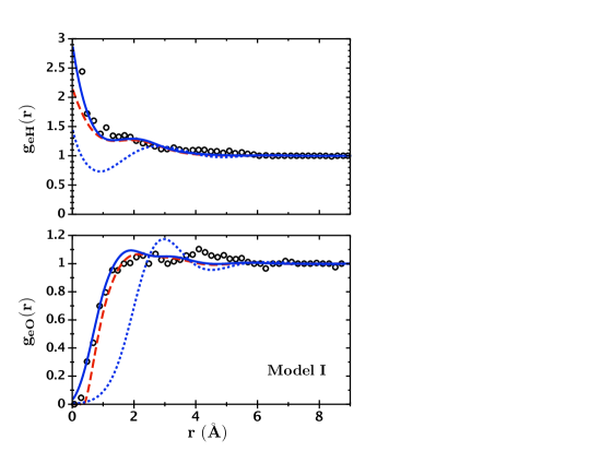
Figure 1: Electron-water site-site radial distribution functions for pseudopotential model I. The blue solid, red dashed and blue dotted lines correspond to theoretical results using the liquid-state equations of DRL, RO-RPA and LWC, respectively. The black circles are simulation data of Sprik et al.Sprik et al. (1986)

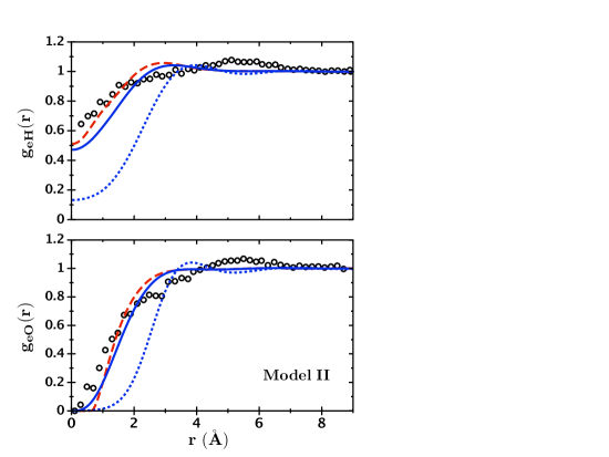
Figure 2: Electron-water site-site radial distribution functions for pseudopotential model II. The blue solid, red dashed and blue dotted lines correspond to theoretical results using the liquid-state equations of DRL, RO-RPA and LWC, respectively. The black circles are simulation data of Sprik et al.Sprik et al. (1986)

The electron-oxygen repulsion in pseudopotential models SR and SR-C is large at short distances. Though not necessary, it was helpful then to solve the DRL equation for this model with respect to a hard-core reference $g_{es}^{ref}(r)$. The RISMChandler and Andersen (1972) predictions for $g_{ss^{\prime}}^{ref}(r)$ and $g_{es}^{ref}(r)$ were used. For model SR, the hard-core diameters were set to be $\sigma_{OO}=2.4$ Å, $\sigma_{OH}=1.4$ Å, $\sigma_{HH}=1.4$ Å, $\sigma_{eO}=0.8$ Å and $\sigma_{eH}=0.0$ Å. For model SR-C the same values were used, except $\sigma_{eO}=1.0$ Å and $\sigma_{eH}=0.5$ Å.

Figure 3 shows results for $g_{es}(r)$ using model SR. As for models I and II, the RO-RPA and DRL-based polaron theories give very similar predictions. The theories predict modest peaks at $r\sim 3$ Å for both $g_{eO}(r)$ and $g_{eH}(r)$, which are not present in the simulation data.Schnitker and Rossky (1987a) The cause appears to be the same as the over-estimation of $g_{es}(r)$ at $r\sim 2.5$ Å for model II, namely the use of the SPC/E water model instead of the SPC to compute the bulk water correlations. Differences in the treatment of the long-range interactions in the MD simulation here and as done by Schnitker and Rossky may also contribute. The theories agree well with the SR data at other distances $r$ though.

As shown in Table 1 the theoretical values for $R_{g}$ for both theories agrees very well with that from simulation, within 4%.Schnitker and Rossky (1987a) The predictions for $\Delta\mu$ are less accurate, being 30% and 23% more negative than the SR estimate for the RO-RPA and DRL-based theories, respectively. Properties using the corrected Schnitker-Rossky pseudopotential, model SR-C, are also shown in the table.

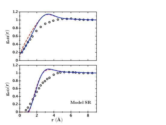
Figure 3: Electron-water site-site radial distribution functions for pseudopotential model SR. The blue solid and red dashed lines correspond to theoretical results using the liquid-state equations of DRL and RO-RPA, respectively. The black circles are simulation data of Schnitker and Rossky.Schnitker and Rossky (1987a)

Figure 4 shows results for $g_{es}(r)$ using model TB. As for the other pseudopotentials, the RO-RPA and DRL-based polaron theories give very similar predictions. Model TB was designed to give greater penetration of the hydrogen cloud by the hydrated electron than the Schnitker-Rossky potential.Turi and Borgis (2002) Comparing $g_{eH}(r)$ in Figures 3 and 4, it appears that Turi and Borgis have been successful. There is no published simulation data for the site-site radial distribution function for model TB.

Table 1 shows that the values of $R_{g}$ predicted by the RO-RPA and DRL theories are less than the simulation value computed by Turi and BorgisTuri and Borgis (2002) by 12% and 9%, respectively. However, as was mentioned above, model TB was optimized for SPC water, not SPC/E. RO-RPA and DRL predictions for $\Delta\mu$ with model TB are more negative than the experimental value by 23% and 15%, respectively.

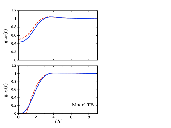
Figure 4: Electron-water site-site radial distribution functions for pseudopotential model TB. The blue solid and red dashed lines correspond to theoretical results using the liquid-state equations of DRL and RO-RPA, respectively.

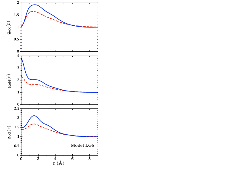
Figure 5: Electron-water site-site radial distribution functions for pseudopotential model LGS. The blue solid and red dashed lines correspond to theoretical results using the liquid-state equations of DRL and RO-RPA, respectively. Site “X” corresponds to the extra site on the water molecule.

Figure 5 shows results for $g_{es}(r)$ using the Larsen, Glover and Schwartz pseudopotential, model LGS. The RO-RPA and DRL-based theories are in qualitative agreement for all correlations. Both show that the water density is increased near the electron,Larsen et al. (2010); Turi and Rossky (2012) with even $g_{eO}(r)$ above unity for all distances $r<8$ Å. The hydrated electron seems to be acting as a source of cohesion for the water in a manner similar to valence electrons in a metal. Contrary to results using the other pseudopotentials though, the RO-RPA and DRL-based theories are not in close quantitative agreement. The reason for this is that while the RO-RPA theory greatly improves correlations between sites that are repulsive, its predictions for correlations between sites that are attractive are only slightly better than for the RPA.Donley et al. (2005) Thus, it is expected that the DRL theory gives a more accurate estimate of these enhanced correlations in model LGS as it does for $g_{eH}(r)$ in model I.

Table 1 shows that the DRL-based theory predicts a value for $R_{g}$ 20% less than simulation, while the RO-RPA prediction equals the simulation value. This agreement between the RO-RPA theory and simulation would seem to be due to a cancellation of errors: it underestimates positive density correlations, which implies an underestimation of the electron-water forces embodied in the medium-induced potential, and this is presumably balanced by an underestimation of the kinetic energy in the reference action, Eq.(II.17).

Perhaps most interestingly, both theories predict an excess chemical potential $\Delta\mu$ that is at least three times more negative than that from experiment. Given the degree of agreement between theory, and simulation and experiment for the other pseudopotential models, this result is surprising. As mentioned above, there are elements in the theory that probably need improvement, such as a better estimate for the electron kinetic energy. Plus, it has been shown that the use of the SPC/E model instead of the SPC does cause noticeable changes in the local correlations and energetics, especially if the handling of the long-range interactions differ. Last, the LGS potential was optimized for SPC water, and it has been shown that the LGS predictions do possess a sensitivity above that of the other potentials.Herbert and Jacobson (2011); Turi and Rossky (2012) So, while it seems unlikely that all these aspects combined could cause an error in $\Delta\mu$ of a factor of three, it should still be considered as possible.

VI Summary and discussion

In summary, the RISM-polaron theory of Chandler and co-workers was improved for the hydrated electron by using two liquid-state theories, RO-RPA and DRL, for the electron-water correlations. It is found that the RO-RPA and DRL-based polaron theories give similar results. Further, for a given pseudopotential, these polaron theories give quantitatively accurate predictions for most static equilibrium properties of the hydrated electron in comparison with path integral Monte Carlo or MD simulations.

One discrepancy between theory and simulation is for the average electron kinetic energy, $\langle ke\rangle$. Evidence presented by othersSumi and Sekino (2004); Wu (1991) appears to point to the cause being the form of the reference action $S_{ref}$, Eq.(II.17), in conjunction with its determination via free energy minimization. Given advances in computing power, a straightforward solution is to compute the path integral directly by Monte Carlo or other means.

It was also discovered that some differences between theory and the quantum/classical simulations were due to using different water models. In that way, a specific electron-water pseudopotential may have meaning only with respect to the water model(s) within which it is optimized. Future comparisons would benefit from implementing the same water model as simulation.

Interestingly, it was found using the LGS pseudopotential that the theories predict that the excess chemical potential, i.e., solvation free energy, is less than -5 eV, that is, at least three times more negative than the experimental value. The LGS prediction for a related quantity, the vertical electron binding energy, has been shown to be almost twice as large as the experimental value.Herbert and Jacobson (2011) So the result here does not stand completely alone. Nonetheless, improvements in the theory are needed to remove uncertainties in the predictions presented here. An estimate of the excess chemical potential using simulation dataSchnitker and Rossky (1987a) would also be helpful.

A simpler approach, using the RPA to model both the electron-water and water-water correlations was also examined. It was found that this RPA theory yielded values for the electron radius of gyration and excess chemical potential that agreed well with experiment even though the RPA predictions for local electron-water and water-water correlations were mediocre. A similar cancellation of effects using an RPA medium-induced potential has been shown for an analogous system, a semi-dilute solution of polyelectrolytes.Donley et al. (1997)

It is noted that the theory can be extended to examine electron excited states by performing an analog of that done in mixed quantum/classical simulations of the hydrated electron. A similar approach has been done for the case in which the water was modeled as a continuum dielectric.Lakhno (2007)

*

Appendix A Numerical solution of the DRL theory

The DRL theory for $g_{es}(r)$ was solved as follows. Given the water structure factors ${\hat{\chi}}_{ss^{\prime}}(k)$, electron intramolecular structure factor ${\hat{\omega}}_{e}(k)$, and initial guesses for the electron-water direct correlation functions ${\hat{c}}_{es}(k)$, the RISM equation, Eq.(II.12), was solved for ${\hat{h}}_{es}(k)$. These functions were then Fourier transformed to obtain $g_{es}(r)$. With these radial distribution functions, the charging integral, Eq.(II.29), was computed using the approximation of Eq.(II.31). New values for $x_{es}(r,1)$ and thus ${\hat{h}}_{es}(k)$ were then obtained using Eq.(II.28).

Define the difference between the nonconverged values of ${\hat{h}}_{es}(k)$ obtained from the two-chain (or approximation thereof) and RISM equations as $\Delta{\hat{h}}_{es}(k)$. Also, define the difference between the new and old solution for ${\hat{c}}_{es}(k)$ as $\Delta{\hat{c}}_{es}(k)$. It can be shown for the LWC approximation Eq.(II.26) to the two-chain equation Eq.(II.22) that the Newton-Raphson solution algorithm gives:

$$\Delta{\hat{c}}_{es}(k)\approx\sum_{s^{\prime}}{\hat{\omega}}_{e}^{-1}(k)\Delta{\hat{h}}_{es^{\prime}}(k){\hat{\omega}}_{s^{\prime}s}^{-1}(k),$$ (A.1)

where ${\hat{\omega}}_{ss^{\prime}}^{-1}(k)$ is the matrix inverse of ${\hat{\omega}}_{ss^{\prime}}(k)$. This expression was used for the DRL theory also. One problem though with Eq.(A.1) for water is that the matrix inverse of ${\hat{\omega}}_{ss^{\prime}}(k)$ becomes singular as $k\rightarrow 0$. This singularity makes the algorithm not very stable. However, a simple solution to this problem was found by cropping ${\hat{\omega}}_{ss^{\prime}}^{-1}(k)$ near $k=0$. This cropping was done by setting the value of ${\hat{\omega}}_{ss^{\prime}}(k)^{-1}$ for $k<k_{min}$ equal to its value at $k_{min}$, which is proportional to the inverse molecule size. For water, $k_{min}\simeq 0.5$ Å^-1.

A new value for ${\hat{c}}_{es}(k)$ was then determined by mixing in a fraction of $\Delta{\hat{c}}_{es}(k)$, this amount being 10-50% typically. This whole procedure was then repeated - with one exception. The one exception is that the value of the charging integral in Eq.(II.29) was held fixed until convergence was obtained on ${\hat{c}}_{es}(k)$. At that time the charging integral was recomputed. A new value for the charging integral was a mixture of its recomputed and old values, typically at a ratio of 1:9. This second outer loop was then continued until convergence on ${\hat{c}}_{es}(k)$ and thus $g_{es}(r)$ was obtained.

Since a variation of Eq.(A.1) is also used for the RO-RPA theory,Donley et al. (2005) this cropping of ${\hat{\omega}}_{ss^{\prime}}^{-1}(k)$ was done for that theory too.

References

- Mozumder (1999) A. Mozumder, Fundamentals of Radiation Chemistry (Academic Press, San Diego, CA, 1999).
- Buxton et al. (1988) G. V. Buxton, C. L. Greenstock, W. P. Helman, and A. B. Ross, J. Phys. Chem. Ref. Data 17, 513 (1988).
- Feng and Kevan (1980) D.-F. Feng and L. Kevan, Chem. Rev. 80, 1 (1980).
- Sprik et al. (1986) M. Sprik, R. W. Impey, and M. L. Klein, J. Stat. Phys. 43, 967 (1986).
- Schnitker and Rossky (1987a) J. Schnitker and P. J. Rossky, J. Chem. Phys. 86, 3471 (1987a).
- Barnett et al. (1988) R. N. Barnett, U. Landman, and A. Nitzan, J. Chem. Phys. 89, 2242 (1988).
- Turi and Borgis (2002) L. Turi and D. Borgis, J. Chem. Phys. 117, 6186 (2002).
- Jacobson and Herbert (2010) L. D. Jacobson and J. M. Herbert, J. Chem. Phys. 133, 154506 (2010).
- Laria et al. (1991) D. Laria, D. Wu, and D. Chandler, J. Chem. Phys. 95, 4444 (1991).
- Turi and Rossky (2012) L. Turi and P. J. Rossky, Chem. Rev. 112, 5641 (2012).
- Larsen et al. (2010) R. E. Larsen, W. J. Glover, and B. J. Schwartz, Science 329, 65 (2010).
- Turi and Madarasz (2011) L. Turi and A. Madarasz, Science 331, 1387 (2011), c.
- Jacobson and Herbert (2011) L. D. Jacobson and J. M. Herbert, Science 331, 1387 (2011), d.
- Larsen et al. (2011) R. E. Larsen, W. J. Glover, and B. J. Schwartz, Science 331, 1387 (2011), e.
- Herbert and Jacobson (2011) J. M. Herbert and L. D. Jacobson, J. Phys. Chem. A 115, 14470 (2011).
- Uhlig et al. (2012) F. Uhlig, O. Marsalek, and P. Jungwirth, J. Phys. Chem. Lett. 3, 3071 (2012).
- Casey et al. (2013) J. R. Casey, R. E. Larsen, and B. J. Schwartz, Proc. Nat. Acad. Sci. USA 110, 2712 (2013).
- Chandler et al. (1984) D. Chandler, Y. Singh, and D. M. Richardson, J. Chem. Phys. 81, 1975 (1984).
- Nichols et al. (1984) A. L. Nichols, D. Chandler, Y. Singh, and D. M. Richardson, J. Chem. Phys. 81, 5109 (1984).
- Hansen and McDonald (1986) J. P. Hansen and I. R. McDonald, Theory of Simple Liquids (Academic Press, London, UK, 1986).
- Schweizer and Curro (1997) K. S. Schweizer and J. G. Curro, Adv. Chem. Phys. 98, 1 (1997).
- Curro et al. (1999) J. G. Curro, E. B. Webb, G. S. Grest, J. D. Weinhold, M. Pütz, and J. D. McCoy, J. Chem. Phys. 111, 9073 (1999).
- Heine et al. (2005) D. R. Heine, G. S. Grest, and J. G. Curro, Adv. Polym. Sci. 173, 209 (2005).
- Donley et al. (2004) J. P. Donley, D. R. Heine, and D. T. Wu, Phys. Rev. E 70, 060201 (2004).
- Donley et al. (1998) J. P. Donley, J. J. Rajasekaran, and A. J. Liu, J. Chem. Phys. 109, 10499 (1998).
- Donley and Heine (2006) J. P. Donley and D. R. Heine, Macromolecules 39, 8467 (2006).
- Note (1) The usual density matrix element is .
- Feynman and Hibbs (2010) R. P. Feynman and A. R. Hibbs, Quantum Mechanics and Path Integrals, emended ed. (Dover Publications, Inc., Mineola, NY, 2010).
- Chandler and Andersen (1972) D. Chandler and H. C. Andersen, J. Chem. Phys. 57, 1930 (1972).
- Melenkevitz et al. (1993) J. Melenkevitz, K. S. Schweizer, and J. G. Curro, Macromolecules 26, 6190 (1993).
- Chandler et al. (1986) D. Chandler, J. D. McCoy, and S. J. Singer, J. Chem. Phys. 85, 5971 (1986).
- Note (2) In the original application of the path integral method to polarons by Feynman, the degrees of freedom of the surrounding crystal were also slow. In that case though, the slow phonon modes were integrated out exactly, they being modeled in the standard way as harmonic oscillators.
- Langer (1971) J. S. Langer, Ann. Phys. (N.Y.) 65, 53 (1971).
- Wu (1991) D. T. Wu, Phd dissertation, University of California, Berkeley, Dept. of Chemistry (1991).
- Sumi and Sekino (2004) T. Sumi and H. Sekino, J. Chem. Phys. 120, 8157 (2004).
- Feynman et al. (1962) R. P. Feynman, R. W. Hellwarth, C. K. Iddings, and P. M. Platzman, Phys. Rev. 127, 1004 (1962).
- Doi and Edwards (1986) M. Doi and S. F. Edwards, Theory of Polymer Dynamics (Oxford University Press, New York, NY, 1986).
- des Cloizeaux and Jannink (1991) J. des Cloizeaux and G. Jannink, Polymers in Solution: Their Modelling and Structure (Oxford University Press, New York, NY, 1991).
- Malescio and Parrinello (1987) G. Malescio and M. Parrinello, Phys. Rev. A 35, 897 (1987).
- Andersen and Chandler (1971) H. C. Andersen and D. Chandler, J. Chem. Phys. 55, 1497 (1971).
- Melenkevitz and Curro (1997) J. Melenkevitz and J. G. Curro, J. Chem. Phys. 106, 1216 (1997).
- Chandler et al. (1982) D. Chandler, R. Silbey, and B. M. Ladanyi, Mol. Phys. 46, 1335 (1982).
- Note (3) In classical statistical mechanics any -site correlation function can be represented exactly as the configurational average of molecules in an effective field.
- Donley et al. (1994) J. P. Donley, J. G. Curro, and J. D. McCoy, J. Chem. Phys. 101, 3205 (1994).
- Note (4) The HNC form of the medium-induced potential was derived. Other forms of the potential as ansatzes have been and can be explored, the only restriction being that they be pairwise decomposable.
- Donley et al. (2005) J. P. Donley, D. R. Heine, and D. T. Wu, Macromolecules 38, 1007 (2005).
- Donley (2002) J. P. Donley, J. Chem. Phys. 116, 5315 (2002).
- Donley (2004) J. P. Donley, J. Chem. Phys. 120, 1661 (2004).
- van der Spoel et al. (1998) D. van der Spoel, P. J. van Maaren, and H. J. C. Berendsen, J. Chem. Phys. 108, 10220 (1998).
- Wu et al. (2006) Y. Wu, H. L. Tepper, and G. A. Voth, J. Chem. Phys. 124, 024503 (2006).
- Plimpton (1995) S. J. Plimpton, J. Comp. Phys. 117, 1 (1995).
- Høye and Stell (1976) J. S. Høye and G. Stell, J. Chem. Phys. 65, 18 (1976).
- Chandler (1977) D. Chandler, J. Chem. Phys. 67, 1113 (1977).
- Schnitker and Rossky (1987b) J. Schnitker and P. J. Rossky, J. Chem. Phys. 86, 3462 (1987b).
- Larsen et al. (2009) R. E. Larsen, W. J. Glover, and B. J. Schwartz, J. Chem. Phys. 131, 037101 (2009).
- Grayce et al. (1994) C. J. Grayce, A. Yethiraj, and K. S. Schweizer, J. Chem. Phys. 100, 6857 (1994).
- Martynov and Sarkisov (1983) G. A. Martynov and G. N. Sarkisov, Mol. Phys. 49, 1495 (1983).
- Note (5) It was not found necessary to weaken the potential even further to attain an effective Percus-Yevick form.
- Bartels et al. (2005) D. M. Bartels, K. Takahashi, J. A. Cline, T. W. Marin, and C. D. Jonah, J. Phys. Chem. A 109, 1299 (2005).
- Jortner and Noyes (1966) J. Jortner and R. M. Noyes, J. Phys. Chem. 70, 770 (1966).
- Note (6) Herbert and JacobsonHerbert and Jacobson (2011), found that employing a more accurate scheme (Ewald sum) than done by LGS to handle the long-range interactions gave Å.
- Donley et al. (1997) J. P. Donley, J. Rudnick, and A. J. Liu, Macromolecules 30, 1188 (1997).
- Lakhno (2007) V. D. Lakhno, Chem. Phys. Lett. 437, 198 (2007).