On the Power Allocation for Hybrid DF and CF Protocol with Auxiliary Parameter in Fading Relay Channels

Abstract

In fading channels, power allocation over channel state may bring a rate increment compared to the fixed constant power mode. Such a rate increment is referred to power allocation gain. It is expected that the power allocation gain varies for different relay protocols. In this paper, Decode-and-Forward (DF) and Compress-and-Forward (CF) protocols are considered. We first establish a general framework for relay power allocation of DF and CF over channel state in half-duplex relay channels and present the optimal solution for relay power allocation with auxiliary parameters, respectively. Then, we reconsider the power allocation problem for one hybrid scheme which always selects the better one between DF and CF and obtain a near optimal solution for the hybrid scheme by introducing an auxiliary rate function as well as avoiding the non-concave rate optimization problem.

I Introduction

In cooperative communication networks, power allocation over channel state may bring rate gains [1]. However, it is not easy to find the optimal power allocation because the exact capacity of most of the wireless networks has not been known. There were some useful cooperation strategies put forward in the literatures which provided efficient approach to transmit information and gave lower bounds for the rate performance of the system. For instance, two relay protocols, Decode-and-Forward (DF) and Compress-and-Forward (CF), were proposed in [2] to evaluate the information rate for relay channels (RC). Particularly, the DF protocol was shown to be able to achieve the capacity of degraded RC [2] and sender frequency division RC [3]. Due to the effectiveness of DF and CF, they has been widely used in cooperative communication networks, achieving good rate performance in various networks [4][5].

Based on DF and CF protocols, power allocation can be naturally extended to general networks to combat the varying channel states. Take the RC as an example again. Since there are only three wireless links in the system, it is available for the source and the relay to know the current channel gains before transmissions via timely feedback from the receiver. The global power allocation over fading channel problem in RC has been studied in [6]. By assuming that the source and the relay subject to a sum power constraint, the authors provided algorithms on how to find the optimal power allocation. It is also noted that the power allocation established in [6] achieved the maximal throughput of the relay-receive phase and relay-transmit phase in half-duplex relay channels (HDRC). The result was implicitly based on a buffer at the relay such that if the relay-destination channel is worse, it can store the message and transmit them when the relay-destination channel becomes better. In practice, if the relay has a finite storage and limited processing capability, the system may become unstable and the power allocation gain will degrade.

To improve the achievable rate, selecting better relay protocol among multiple protocols provides another alternative. This intuition comes from theoretical analysis on combining DF and CF in static RC [7]-[9]. It was found superposition structure of the DF and CF codewords provides some rate gain with penalties of decoding complexity [2][10]. Moreover, a general insight was also obtained that DF outperforms CF for only some of the channel gain combinations while the relationship reverses for the others. This implies that in fading relay channels, a hybrid scheme which selects the better one between DF and CF according to the channel state may provide some rate gains while avoiding the complicated codeword design.

Instead of using other techniques, e.g., [11]-[13], to combat channel fading, in this work, we thoroughly analyze the relay power allocation over channel state when the relay adopts both DF and CF protocols.

The remainder of this paper is organized as follows. In Section II, we introduce the system model and establish a general framework for the relay power allocation problem. In Section III, we present a parameterized form solution for the problem corresponding to DF and CF, respectively. In Section IV, we further investigate the relay power allocation corresponding to the hybrid scheme and discuss the optimal solution by introducing an auxiliary rate function.

II System model and problem preliminary

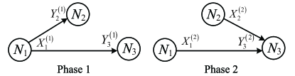
Figure 1: The two-phase transmission of a half-duplex relay channel.

Let us consider a HDRC as illustrated in Fig. 1. In the figure, $N_{1}$, $N_{2}$ and $N_{3}$ represent the source, the relay and the destination, respectively. We assume the relay is operated in half-duplex manner. Due to the multipath effect, the channel gains are varying along with the time. We assume that the channel gains are holding constant for a fixed time length which is referred to as a block and the channel gains varies independently between consecutive blocks. The signal transmissions in each block are divided into two phases as depicted in Fig. 1. In Phase 1, the source transmits signal while the other two nodes listen. In Phase 2, the source and the relay transmit signals to the destination. To distinguish the signal in different phases, let us denote the complex baseband signal transmitted at $N_{i}~{}(i=1,2)$ and received at $N_{j}~{}(j=2,3)$ in Phase $k$ $(k=1,2)$ by $X_{i}^{(k)}$ and $Y_{j}^{(k)}$, respectively. For simplicity, we use $H_{ji}$ and $h_{ji}$ to represent the channel gain variable and its realization for $N_{i}$-$N_{j}$ link in each block. Accordingly, transmissions in the HDRC can be expressed as

$$Y_{3}^{(1)}= ~{}h_{31}X_{1}^{(1)}+Z_{3}^{(1)}$$ (1)

$$Y_{2}^{(1)}= ~{}h_{21}X_{1}^{(1)}+Z_{2}^{(1)}$$ (2)

$$Y_{3}^{(2)}= ~{}h_{31}X_{1}^{(2)}+h_{32}X_{2}^{(2)}+Z_{3}^{(2)}$$ (3)

where $Z_{j}^{(k)}~{}(j=2,3;~{}k=1,2)$ is additive white Gaussian noise (AWGN) corresponding to $N_{j}$ in Phase $k$. For simplicity, we consider that the system is operated in unit bandwidth and we assume that $Z_{j}^{(k)}$ obeys complex Gaussian distribution with unit power spectrum density, i.e., $Z_{j}^{(k)}\sim\mathcal{CN}(0,1)$. The source and the relay are assumed to know the channel gains at the beginning of each block. In particular, as the channel phase-shift is well-recovered at the receiver side, we focus on $p_{{}_{|H_{ji}|}}(|h_{ji}|)$, the distribution of the amplitude of $H_{ji}$.

For the reason of synchronization and power management, we assume that the source transmit signal with the same power and the same time length for the two phases. Denote the channel state by $\vec{h}=(h_{31},h_{21},h_{32})$. By assuming that the block length is long enough to support one time entire signalling, we can regard the system as a static relay channel for each block. In general, in the static case, the rate performance is a function of the receiver side signal to noise ratio (SNR) of the three links. To focus on the relay power allocation, we denote the receiver side SNR of relay-destination link and the rate function in static HDRC by $S_{2}\triangleq 2|h_{32}|^{2}P_{2}$ and $R(S_{2})$, respectively.

In fading HDRC, we consider long time average power constraint $\overline{P_{i}}$ at $N_{i}~{}(i=1,2)$. Then the source transmits signal with power $\overline{P_{1}}$ regardless of the channel state. However, the relay can adjust $P_{2}$ adaptively w.r.t the channel state $\vec{h}$ in each block. For clarity, we denote the relay power allocation by $P_{2}(\vec{h})$. The interest of this paper is to find the optimal power allocation $P_{2}^{\star}(\vec{h})$ achieving the best rate performance of the system. Define $S_{2}(\vec{h})\triangleq 2|h_{32}|^{2}P_{2}(\vec{h})$. Regarding the average rate as the measurement of the rate performance and taking the average power constraint into consideration, we can specify the relay power allocation problem as

$$\mathcal{P}:~{}~{}~{}~{} \max_{S_{2}(\vec{h})}~{}~{}\left(\int_{0}^{\infty}\right)^{3}p(\vec{h})R(S_{2}(\vec{h}))d\vec{h}$$ (4)

$$\text{~{}~{}s.t.}~{}~{}~{}\left(\int_{0}^{\infty}\right)^{3}p(\vec{h})\frac{S_{2}(\vec{h})}{2|h_{32}|^{2}}d\vec{h}=\overline{P_{2}},$$ (5)

where $p(\vec{h})=p_{{}_{|H_{31}|}}(|h_{31}|)p_{{}_{|H_{21}|}}(|h_{21}|)p_{{}_{|H_{32}|}}(|h_{32}|)$; $\left(\int_{0}^{\infty}\right)^{3}\triangleq\int_{0}^{+\infty}\int_{0}^{+\infty}\int_{0}^{+\infty}$; and $\mathrm{d}\vec{h}\triangleq\mathrm{d}|h_{31}|\mathrm{d}|h_{21}|\mathrm{d}|h_{32}|$.

If $R(S_{2})$ is concave w.r.t. $S_{2}$, one can solve $\mathcal{P}$ by Lagrangian method. Consider the Lagrangian

$$\mathcal{L}(S_{2}(\vec{h}),\mu)=\left(\int_{0}^{\infty}\right)^{3}p(\vec{h})R(S_{2}(\vec{h}))d\vec{h}\\ -\mu\bigg{(}\left(\int_{0}^{\infty}\right)^{3}p(\vec{h})\frac{S_{2}(\vec{h})}{2|h_{32}|^{2}}d\vec{h}-\overline{P_{2}}\bigg{)}.$$ (6)

Set $\frac{\partial\mathcal{L}(S_{2}(\vec{h}),\mu)}{\partial S_{2}(\vec{h})}=0$. One has

$$\frac{\mathrm{d}R(S_{2}(\vec{h}))}{\mathrm{d}S_{2}(\vec{h})}-\frac{\mu}{2|h_{32}|^{2}}=0.$$ (7)

It should be noted that only if the rate function $R(S_{2})$ is concave w.r.t. $S_{2}$ should the solution of (7) be the optimal $S_{2}(\vec{h})$.

III Optimal power allocation for DF and CF strategies

In this section, we first analyze the concavity of DF rate and CF rate. Then following necessary condition (7), we present the optimal power allocation for DF and CF based on the inverse function of the derivation of the rates.

III-A Concavity of the DF rate and CF rate

The rate achieved by DF protocol and CF protocol with Gaussian signaling were presented in Proposition 2 and Proposition 3 of [6], respectively. Taking a constant fixed source power and the equal-phase assumption into account, the DF rate can be rewritten as

$$\frac{1}{2}\max\limits_{0\leq\rho\leq 1}\min\big{\{}C(|h_{21}|^{2}P_{1})+C\big{(}\overline{\rho^{2}}|h_{31}|^{2}P_{1}\big{)},C(|h_{31}|^{2}P_{1})$$

$$~{}~{}~{}+C(|h_{31}|^{2}P_{1}+2|h_{32}|^{2}P_{2}+2\rho\sqrt{2|h_{31}|^{2}P_{1}|h_{32}|^{2}P_{2}})\big{\}},$$

where $\overline{\rho^{2}}=1-\rho^{2}$; $C(x)\triangleq\log_{2}(1+x)$ represents the Shannon formula for complex based model [1]; $\rho$ represents the correlation coefficient of $X_{1}^{(1)}$ and $X_{2}^{(2)}$. Similarly, the CF rate can be expressed as

$$\frac{1}{2}C(h_{31}^{2}P_{1})+\frac{1}{2}C\Big{(}h_{31}^{2}P_{1}+\frac{2h_{21}^{2}P_{1}h_{32}^{2}P_{2}}{1+h_{21}^{2}P_{1}+h_{31}^{2}P_{1}+2h_{32}^{2}P_{2}}\Big{)}.$$

Define

$$S_{1}\triangleq|h_{31}|^{2}P_{1};~{}t\triangleq|h_{31}|^{2}/|h_{31}|^{2}.$$

Then we can further express the DF rate and CF rate as functions of $S_{2}$:

$$R_{DF}(S_{2})= \frac{1}{2}\max\limits_{0\leq\rho\leq 1}\min\big{\{}C(tS_{1})+C(\overline{\rho^{2}}S_{1}),$$

$$~{}~{}~{}~{}~{}~{}~{}~{}C(S_{1})+C(S_{1}+S_{2}+2\rho\sqrt{S_{1}S_{2}})\big{\}},$$ (8)

$$R_{CF}(S_{2})= \frac{C(S_{1})}{2}+\frac{1}{2}C\Big{(}S_{1}+\frac{tS_{1}S_{2}}{1+(t+1)S_{1}+S_{2}}\Big{)}.$$ (9)

Theorem 1

Both the DF rate $R_{DF}(S_{2})$ and CF rate $R_{CF}(S_{2})$ are concave w.r.t. $S_{2}$.

Proof: First, we analyze the concavity of $R_{DF}(S_{2})$. In $R_{DF}(S_{2})$, the optimal $\rho$ can be found by considering

$$C(tS_{1})+C(\overline{\rho^{2}}S_{1})=C(S_{1})+C(S_{1}+S_{2}+2\rho\sqrt{S_{1}S_{2}})$$

which results in

$$\rho=\frac{\sqrt{S_{2}+\eta(tS_{1}-S_{1}-S_{2})}-\sqrt{S_{2}}}{\eta\sqrt{S_{1}}}\triangleq\rho^{*}$$ (10)

where $\eta\triangleq(1+tS_{1})/(1+S_{1})$. Note that the first and the second terms in the minimum operation of (8) are monotonically decreasing and increasing w.r.t. $\rho$, $\rho\in[0,1]$. Then we have

$$R_{DF}(S_{2})=\frac{1}{2}C(S_{1})+\frac{1}{2}\min\big{\{}C(tS_{1}),\\ C\big{(}(\sqrt{S_{1}}+\sqrt{S_{2}})^{2}\big{)},C(S_{1}+S_{2}+2\rho^{*}\sqrt{S_{1}S_{2}})\big{\}}$$ (11)

As minimum operation is a concavity-preserving [14], to show $R_{DF}(S_{2})$ is concave, we only need to show all the three terms in the minimum operation are concave. The concavity of $C(tS_{1})$ is trivial. Note that logarithmic function is concave. According to the composition law of concavity, to show the rest two terms in (11) are concave, it is equivalent to show $(\sqrt{S_{1}}+\sqrt{S_{2}})^{2}$ and

$$g_{d}(S_{2})\triangleq S_{1}+S_{2}+2\rho^{*}\sqrt{S_{1}S_{2}}$$

are concave w.r.t. $S_{2}$ [14]. On the one hand, it is not hard to see

$$\frac{\mathrm{d}[(\sqrt{S_{1}}+\sqrt{S_{2}})^{2}]}{\mathrm{d}S_{2}}=-\frac{\sqrt{S_{1}}}{2S_{2}\sqrt{S_{2}}}<0$$

which implies the concavity of $(\sqrt{S_{1}}+\sqrt{S_{2}})^{2}$. On the other hand, with some manipulations, one has

$$g_{d}(S_{2})= S_{1}+S_{2}+\frac{2}{\eta}\Big{(}\sqrt{S_{2}^{2}+\eta(tS_{1}-S_{1}-S_{2})S_{2}}-S_{2}\Big{)},$$

$$g_{d}^{\prime}(S_{2})= 1-\frac{2}{\eta}+\frac{2(1-\eta)S_{2}+\eta(tS_{1}-S_{1})}{\eta\sqrt{S_{2}^{2}+\eta(tS_{1}-S_{1}-S_{2})S_{2}}},$$ (12)

$$g_{d}^{\prime\prime}(S_{2})= \frac{2(1-\eta)}{\eta\sqrt{S_{2}^{2}+\eta(tS_{1}-S_{1}-S_{2})S_{2}}}$$

$$-\frac{[2(1-\eta)S_{2}+\eta(tS_{1}-S_{1})]^{2}}{2\eta[S_{2}^{2}+\eta(tS_{1}-S_{1}-S_{2})S_{2}]^{\frac{3}{2}}}$$

$$= \frac{-[\eta(tS_{1}-S_{1})]^{2}}{2\eta[S_{2}^{2}+\eta(tS_{1}-S_{1}-S_{2})S_{2}]^{\frac{3}{2}}}\leq 0.$$

That is, $g_{d}(S_{2})$ is also concave. This implies the concavity of the DF rate $R_{DF}(S_{2})$.

Next, we show that $R_{CF}(S_{2})$ is concave. Let us define

$$g_{c}(S_{2})\triangleq 1+S_{1}+\frac{tS_{1}S_{2}}{1+(t+1)S_{1}+S_{2}}.$$

Then

$$R_{CF}(S_{2})=\frac{1}{2}C(S_{1})+\frac{1}{2}\log_{2}[g_{c}(S_{2})].$$

According to the composition law of concavity [14], it is equivalent to show that $g_{c}(S_{2})$ is concave. Note that

$$g_{c}^{\prime}(S_{2})= \frac{tS_{1}[1+(t+1)S_{1}]}{[1+(t+1)S_{1}+S_{2}]^{2}},$$ (13)

$$g_{c}^{\prime\prime}(S_{2})= \frac{-2tS_{1}[1+(t+1)S_{1}]}{[1+(t+1)S_{1}+S_{2}]^{3}}<0.$$

Then the CF rate $R_{CF}(S_{2})$ is concave w.r.t. $S_{2}$.

III-B Optimal power allocation corresponding to DF and CF

As both the DF rate and CF rate are concave w.r.t. $S_{2}$, one can derive the optimal relay power allocation according to the necessary condition (7) by well-defining the reverse function of $R_{DF}^{\prime}(S_{2})$ and $R_{CF}^{\prime}(S_{2})$.

For $\sigma\in\{DF,CF\}$, let us denote the reverse function of $R_{\sigma}^{\prime}(S_{2})$ by $T_{\sigma}(\nu)$. We have the following theorem on the power allocation corresponding to DF and CF.

Theorem 2

For $\sigma\in\{DF,CF\}$, the optimal relay power allocation corresponding to protocol $\sigma$ is given by

$$P_{2,\sigma}^{\star}(\vec{h})=S_{2,\sigma}^{\star}(\vec{h})/(2|h_{32}|^{2})\triangleq\frac{1}{2|h_{32}|^{2}}T_{\sigma}\Big{(}\frac{\mu^{\star}_{\sigma}}{2|h_{32}|^{2}}\Big{)}$$ (14)

where $\mu_{\sigma}^{\star}$ satisfies (5).

Proof:  The solution can be naturally derived from (7) by regarding it as an equation of $S_{2}$. Further noting that $S_{2}(\vec{h})=2|h_{32}|^{2}P_{2}(\vec{h})$, we can express the optimal power allocation corresponding to strategy $\sigma$ as (23). $\hfill\blacksquare$

Next, let us analyze $T_{CF}(\nu)$ and $T_{DF}(\nu)$ in detail.

First, it is straightforward to see

$$R_{CF}^{\prime}(S_{2})= \frac{g_{c}^{\prime}(S_{2})}{2g_{c}(S_{2})\ln 2}=\frac{t[1+(t+1)S_{1}]}{2[1+(t+1)S_{1}+S_{2}]^{2}g_{c}(S_{2})\ln 2}.$$

In fact, $[1+(t+1)S_{1}+S_{2}]^{2}g_{c}(S_{2})$ is a quadratic polynomial w.r.t $S_{2}$. Then $T_{CF}(\nu)$ can be expressed as the positive solution of quadratic equation in $S_{2}$:

$$[1+(t+1)S_{1}+S_{2}]^{2}g_{c}(S_{2})=\frac{t[1+(t+1)S_{1}]}{2\nu\ln 2}.$$

According to (11), $R_{DF}(S_{2})$ is a continuous piecewise function. Due to that $R_{DF}^{\prime}(S_{2})$ is not continuous, analysis on $T_{DF}(\nu)$ becomes complicated. By comparing the three terms in (11), it is not hard to rewrite $R_{DF}(S_{2})$ in a piecewise form as

$$R_{DF} (S_{2})=\frac{1}{2}C(S_{1})+$$

$$\begin{cases}\frac{1}{2}C\big{(}(\sqrt{S_{1}}+\sqrt{S_{2}})^{2}\big{)},&\rho^{*}>1\\ \frac{1}{2}C(S_{1}+S_{2}+2\rho^{*}\sqrt{S_{1}S_{2}}),&\rho^{*}\in[0,1]\\ \frac{1}{2}C(tS_{1}),&\rho^{*}<0\end{cases}$$ (15)

In fact, if $t>1$, then $\rho^{*}>1$ is equivalent to

$$\sqrt{S_{2}+\eta(tS_{1}-S_{1}-S_{2})}-\sqrt{S_{2}}>\eta\sqrt{S_{1}}$$

That is,

$$tS_{1}-S_{1}-S_{2}>\eta S_{1}+2\sqrt{S_{1}S_{2}}.$$

If $t-\eta>1$, or equivalently $t>S_{1}+2$, it arrives that

$$S_{2}<S_{1}(\sqrt{t-\eta}-1)^{2}\triangleq f_{1}(S_{1}).$$ (16)

Similarly, if $t>1$, then $\rho^{*}<0$ is equivalent to

$$S_{2}>(t-1)S_{1}\triangleq f_{2}(S_{1}).$$ (17)

After some manipulations, we have

$$R_{DF}^{\prime}(S_{2})=$$

$$\begin{cases}\frac{\sqrt{S_{1}/S_{2}}+1}{2(1+S_{1}+S_{2}+2\sqrt{S_{1}S_{2}})\ln 2},&0<S_{2}<f_{1}(S_{1}),\\ \frac{g_{d}^{\prime}(S_{2})}{2(1+S_{1}+S_{2}+2\rho^{*}\sqrt{S_{1}S_{2}})\ln 2}.&f_{1}(S_{1})<S_{2}<f_{2}(S_{1}),\\ 0,&S_{2}>f_{2}(S_{1})\end{cases}$$ (18)

It is easy to verify that $g_{d}^{\prime}[f_{2}(S_{1})]=0$. Hence, $R_{DF}^{\prime}[f_{2}^{+}(S_{1})]=R_{DF}^{\prime}[f_{2}^{-}(S_{1})]=0$ and $R_{DF}^{\prime}[f_{2}(S_{1})]=0$. However, with some manipulations, one can show that $g_{d}^{\prime}[f_{1}(S_{1})]<\sqrt{S_{1}/f_{1}(S_{1})}+1$. Accordingly, $R_{DF}^{\prime}[f_{1}^{+}(S_{1})]<R_{DF}^{\prime}[f_{1}^{-}(S_{1})]$ and $R_{DF}^{\prime}[f_{1}(S_{1})]$ does not exist. According to these analysis, we can define the reverse function of $R_{DF}^{\prime}(S_{2})$ as follows.

• If

  $$0\leq\nu<\frac{g_{d}^{\prime}[f_{1}(S_{1})]}{2(1+[\sqrt{S_{1}}+\sqrt{f_{1}(S_{1})}]^{2})\ln 2},$$

  then $T_{DF}(\nu)$ is set to the solution of equation in $S_{2}$:

  $$g_{d}^{\prime}(S_{2})=2(1+S_{1}+S_{2}+2\rho^{*}\sqrt{S_{1}S_{2}})\nu\ln 2.$$

• If

  $$\nu>\frac{\sqrt{S_{1}/f_{1}(S_{1})}+1}{2(1+[\sqrt{S_{1}}+\sqrt{f_{1}(S_{1})}]^{2})\ln 2},$$

  then $T_{DF}(\nu)$ is set to the solution of equation regarding of $S_{2}$

  $$\sqrt{S_{1}/S_{2}}+1=2(1+S_{1}+S_{2}+2\sqrt{S_{1}S_{2}})\nu\ln 2.$$

• Otherwise, $T_{DF}(\nu)$ is set to $f_{1}(S_{1})$.

With the definition of $T_{\sigma}(\nu)~{}(\sigma\in\{DF,CF\})$, one can search for $\nu_{\sigma}^{\star}$ in Theorem (2). This not only helps implementation for power allocation but also provides clues for analyzing the power allocation in combining DF and CF protocols.

IV Optimal power allocation based on selecting the better one between DF and CF

As stated previously, the protocol with selecting a better rate between DF and CF can be expressed as

$$R(S_{2})\triangleq\max\{R_{DF}(S_{2}),R_{CF}(S_{2})\}.$$

Then, in a static relay channel, $R(S_{2})$ is achievable by switching to the better one between DF and CF protocols according to the channel gains.

The selection is significant by noting that if $t>1$, neither DF nor CF outperforms the other for all the relay power. Define

$$f(S_{1})\triangleq(t-1)\big{(}1+(t+1)S_{1}\big{)}.$$ (19)

One can easily verify that, if $S_{2}>f(S_{1})$, then $R_{CF}(S_{2})>R_{DF}(S_{2})$ and if $S_{2}<f(S_{1})$, then $R_{CF}(S_{2})>R_{DF}(S_{2})$. Accordingly, we have

$$R(S_{2})=\begin{cases}R_{DF}(S_{2}),&S_{2}\leq f(S_{1})\\ R_{CF}(S_{2}),&S_{2}>f(S_{1}).\end{cases}$$ (20)

It is noted that

$$R^{\prime}[f^{+}(S_{1})]=R_{CF}^{\prime}[f(S_{1})]\\ >0=R_{DF}^{\prime}[f(S_{1})]=R^{\prime}[f^{-}(S_{1})].$$ (21)

Therefore, $R(S_{2})$ is not concave w.r.t. $S_{2}$ anymore. In a fading HDRC, we cannot use (7) to find the optimal power allocation corresponding to $R(S_{2})$ as what we have done for the case using DF/CF protocol. To find some possible solutions, let us introduce the concave envelops of $R(S_{2})$, $\overline{R}(S_{2})$. In general, $\overline{R}(S_{2})\geq R(S_{2})$ for all $S_{2}\geq 0$ and $\overline{R}(S_{2})$ is concave. Particularly, for any concave function $\tilde{R}(S_{2})$ satisfying $\tilde{R}(S_{2})\geq R(S_{2})$ for all $S_{2}\geq 0$, one has $\tilde{R}(S_{2})\geq\overline{R}(S_{2})$.

As both $R_{DF}(S_{2})$ and $R_{CF}(S_{2})$ are concave and monotonically increasing functions of $S_{2}$, it is easy to deduce that $\overline{R}(S_{2})$ is made up of three parts: a curve coincident with $R_{DF}(S_{2})$, a line segment connecting two points and another curve coincident with $R_{CF}(S_{2})$. In particular, the two end points of the line segment should be located on $R_{DF}(S_{2})$ and $R_{CF}(S_{2})$, respectively. What’s more, if $R_{\sigma}(S_{2})~{}(\sigma\in\{DF,CF\})$ is smooth at the end point, the line segment should be tangent with $R_{\sigma}(S_{2})$. Assume the two end points of the line segment are $(S_{d},R_{DF}(S_{d}))$ and $(S_{c},R_{CF}(S_{c}))$, respectively where $S_{d}<S_{c}$. Then, the slope of the line segment is given by

$$K\triangleq\frac{R_{CF}(S_{c})-R_{DF}(S_{d})}{S_{c}-S_{d}}.$$

Besides, it also has $\overline{R}^{\prime}(S_{c}^{+})\leq K\leq\overline{R}^{\prime}(S_{d}^{-})$. Accordingly, we can express $\overline{R}(S_{2})$ as

$$\overline{R}(S_{2})=\begin{cases}R_{DF}(S_{2}),&0<S_{2}\leq S_{d}\\ R_{DF}(S_{d})+K(S_{2}-S_{d}),&S_{d}<S_{2}\leq S_{c}\\ R_{CF}(S_{2}),&S_{2}>S_{c}.\end{cases}$$

Naturally, the derivation of $\overline{R}(S_{2})$ can be expressed as

$$\overline{R}^{\prime}(S_{2})=\begin{cases}R_{DF}^{\prime}(S_{2}),&0<S_{2}<S_{d}\\ K,&S_{d}<S_{2}<S_{c}\\ R_{CF}^{\prime}(S_{2}),&S_{2}>S_{c}.\end{cases}$$ (22)

Let us denote the reverse function of $\overline{R}^{\prime}(S_{2})$ by $T(\nu)$. If $S_{d}<S_{2}<S_{c}$, then $\overline{R}(S_{2})=K$ always holds. Therefore, one can define uncountable version of $T(\nu)$. Similar to the definition of $T_{DF}(\nu)$, let us define $T(\nu)$ as follows.

• If there is a non-empty set $\mathcal{S}$ satisfying that for each $S_{2}\in\mathcal{S}$, $\overline{R}^{\prime}(S_{2}^{+})\leq\nu\leq\overline{R}^{\prime}(S_{2}^{-})$ holds, then $T(\nu)$ is set to the infimum of $\mathcal{S}$.

• Otherwise, set $T(\nu)=0$.

It can be readily seen from the definition of $T(\nu)$ that the smallest receiver side SNR of the relay-destination link, or equivalently, the least relay power, is selected among those satisfying the necessary condition (7). In fact, for $T(\nu)<S_{d}$ and $T(\nu)>S_{c}$, this definition of $T(\nu)$ is the same as that of $T_{DF}(\nu)$ and $T_{CF}(\nu)$, respectively. This specific definition of $T(\nu)$ induces a near optimal solution for power allocation based on $R(S_{2})$. We summarize the result in following theorem.

Theorem 3

Given

$$P_{2}^{\star}(\vec{h})=S_{2}^{\star}(\vec{h})/(2|h_{32}|^{2})\triangleq\frac{1}{2|h_{32}|^{2}}T\Big{(}\frac{\mu^{\star}}{2|h_{32}|^{2}}\Big{)}$$ (23)

where $\mu^{\star}$ satisfies (5). Then $P_{2}^{\star}(\vec{h})$ is a near optimal solution for relay power allocation problem $\mathcal{P}$ based on $R(S_{2})$ which is achieved by selecting the better protocol between DF and CF.

Proof: Similar to what we have done for $R_{DF}(S_{2})$ and $R_{CF}(S_{2})$, if we use $\overline{R}(S_{2})$ as the static rate performance of the system, we can get an optimal power allocation $P_{2}^{\star}(\vec{h})$ following from (7) and $T(\nu)$. $\hfill\blacksquare$

Interestingly, the obtained average rate corresponding to $\overline{R}(S_{2}(\vec{h}))$ also can be achieved by ${R}(S_{2}(\vec{h}))$ since $\overline{R}(S_{2}(\vec{h}))=R(S_{2}(\vec{h}))$ holds for the solution $S_{2}(\vec{h})$. This can be verified by noting that $\overline{R}(S_{2})>R(S_{2})$ holds if and only if $S_{d}<S_{2}<S_{c}$. In fact, for any $S_{2}$ satisfying $S_{d}\leq S_{2}\leq S_{c}$, it has $\overline{R}^{\prime}(S_{2}^{+})\leq K\leq\overline{R}^{\prime}(S_{2}^{-})$ and $T(K)=S_{d}$.

Due to the fact that $\overline{R}(S_{2})\geq R(S_{2})$ holds in general, the obtained power allocation can guarantee a near-optimal rate performance.$\hfill\square$

V Conclusion

We investigated relay power allocation over channel state in fading HDRC based on both DF protocol and CF protocol. By proving the concavity of the DF rate and CF rate, a parameterized form solution for the optimal power allocation has been presented. Furthermore, we considered a hybrid DF and CF protocol and introduced an auxiliary function which helped find a near optimal solution of the corresponding relay power allocation problem.

References

• [1] Thomas M. Cover, Joy A. Thomas, “Elements of Information Theory,” Second Edition, John Wiley and Sons, 2006.
• [2] T. Cover and A. El Gamal, “Capacity theorems for the relay channel,” IEEE Trans. Inform. Theory, vol. 25, No. 5, pp. 572-584, Sept. 1979.
• [3] A. El Gamal and S. Zahedi, “Capacity of a class of relay channels with orthogonal components”, IEEE Trans. Inform. Theory, vol. 51, no. 5, pp. 1815-1817, May 2005.
• [4] G. Kramer, M. Gastpar, and P. Gupta, “Cooperative strategies and capacity theorems for relay networks,” IEEE Trans. Inform. Theory, vol. 51, no. 9, pp. 3037-3063, Sept. 2005.
• [5] S. H. Lim, Y.-H. Kim, A. El Gamal and S.-Y. Chung, “Noisy network coding”, IEEE Trans. Inform. Theory, vol. 57, no. 5, pp. 3132-3152, May 2011.
• [6] A. Host-Madsen and J. Zhang, “Capacity bounds and power allocation for wireless relay channels,” IEEE Trans. Inform. Theory, vol. 51, no. 6, pp. 2020-2040, June 2005.
• [7] Z. Chen, P. Fan and K. B. Letaief, “Subband division for Gaussian relay channel”, in Proceedings of the IEEE International Conference on Communications (ICC), 2014, pp. 5438-5442.
• [8] Z. Chen, P. Fan and K. B. Letaief, “SNR Decomposition for Gaussian Relay channel,” to appear in IEEE Trans. Wireless Commun..
• [9] Z. Chen, P. Fan, D. Wu, K. Xiong and K. B. Letaief, “On the Achievable Rates of Full-duplex Gaussian Relay Channel,” in Proceedings of the IEEE Global Communication Conference (Globecom), 2014.
• [10] H. F. Chong, and M. Motani, “On Achievable Rates for the General Relay Channel,” IEEE Trans. Inform. Theory, vol. 57, no. 3, pp. 1249-1266, Mar. 2011.
• [11] D. Zhang, P. Fan and Z. Cao. “Interference cancellation for OFDM systems in presence of overlapped narrow band transmission system”. IEEE Transactions on Consumer Electronics, vol. 50, no. 1, pp. 108-114, 2004.
• [12] J. Kang. P. Fan and Z. Cao. “Flexible construction of irregular partitioned permutation LDPC codes with low error floors”. IEEE Communication Letters, vol. 9, no. 6, pp. 534-536, 2005.
• [13] H. Chan, P. Fan and Z. Cao. “A utility-based network selection scheme for multiple services in heterogeneous networks”. in 2005 Proceedings of International Conference on Wireless Networks, Communications and Mobile Computing, vol. 2, pp. 1175-1180, 2005.
• [14] S. Boyd and L. Vandenberghe, “Convex Optimization,” Cambridge Univ. Press, U.K. 2003.